Anomalous and linear holographic hard wall models
for light unflavored mesons

Abstract

In this work we consider anomalous and linear holographic hard wall (HW) models for light unflavored mesons inspired by the AdS/CFT correspondence. The anomalous dimensions depend on the logarithm of the spin $S$ of the meson state and come from a semiclassical analysis of gauge/string duality. The anomalous HW model produces very good masses and good Regge trajectories for mesons compared with PDG data. Inspired by this anomalous HW model we also propose a phenomenological modification of the dimension of the boundary operators such that the model produces asymptotic linear Regge trajectories.

I Introduction

The AdS/CFT correspondence Aharony:1999ti establishes relations between Yang-Mills (YM) and higher dimensional gravitational theories. One of the amazing properties of the correspondence is that if YM theories are strongly coupled, the gravitational one is weak coupled allowing for the solution of a myriad of phenomena from the quark-gluon plasma to condensed matter (for reviews, see e.g., Casalderrey-Solana:2011dxg ; Zaanen:2015oix ). In particular, hadronic spectra were described by different proposals as the holographic hard wall (HW) and the soft wall (SW) models Boschi-Filho:2002xih ; Boschi-Filho:2002wdj ; deTeramond:2005su ; Erlich:2005qh ; Boschi-Filho:2005xct ; Karch:2006pv ; Colangelo:2008us . The HW model Boschi-Filho:2002xih ; Boschi-Filho:2002wdj ; deTeramond:2005su ; Erlich:2005qh ; Boschi-Filho:2005xct is well known for producing reasonable hadronic masses but non-linear (parabolic) Regge trajectories. On the other side, the SW model Karch:2006pv ; Colangelo:2008us also give good masses with the advantage of generating linear Regge trajectories.

In this work, we are going to consider the inclusion of anomalous dimensions for the boundary operators describing light unflavored mesons with spins $S\geq 1$. These anomalous dimensions depend on the logarithm of the spin $S$ of the mesonic state inspired by a semiclasical analysis of gauge/string dualities Gubser:2002tv and was used recently to discuss the case of even spins glueballs Costa-Silva:2023vuu . We find very good masses and Regge trajectories for the studied mesons when compared with PDG data PDG:2022pth , better than the ones from the HW and SW models. Furthermore, we discuss a phenomenological modification of the dimension of the boundary operators representing the mesonic states in order to obtain asymptotic linear Regge trajectories, similar to the case of glueballs. Actually, the linearization of the mesonic states require an additional parameter to obtain the best fit to PDG data. For a recent account on non-holographic meson Regge trajectories, see e.g. Chen:2021kfw .

This work is organized as follows. In Section II, we review the HW model for light unflavored mesons and in Section III we discuss the introduction of anomalous dimensions in the HW model and obtain the spectra for the mesonic families starting with the states of the $\rho(770)$, $\omega(782)$, $b_{1}(1235)$, and $h_{1}(1170)$. Then, in Section IV we modify the dimension of the mesonic boundary operators such that we find asymptotic linear Regge trajectories for the mesons already discussed in the previous section. Finally, in Section V we present our conclusions.

II Original HW model for mesons

In this work we are interested in studying the spectra of light unflavored mesons, and their Regge trajectories using anomalous and linear holographic HW models. These mesons can be classified in four families according to their behavior under $\mathcal{CP}$ transformations (even or odd), isospin $I=0$ and $1$, and spins $S\geq 1$. These four families imply four distinct Regge trajectories.

In order to describe such objects using the holographic HW model, we need to study a massive vector field in $AdS_{5}$. We start with the action

$$S=-\frac{1}{2}\int d^{5}x\sqrt{-g}\bigg{[}\frac{1}{2}g^{pm}g^{qn}F_{mn}F_{pq}+M_{5}^{2}g^{pm}A_{p}A_{m}\bigg{]},$$ (1)

where $F_{mn}=\partial_{m}A_{n}-\partial_{n}A_{m}$ is the stress tensor of the Proca field with mass $M_{5}$ in the five-dimensional AdS space. Moreover, $g$ is the determinant of the metric of $AdS_{5}$,

$$ds^{2}=g_{mn}dx^{m}dx^{n}=\frac{R^{2}}{z^{2}}(dz^{2}+\eta_{\mu\nu}dx^{\mu}dx^{\nu}),$$ (2)

with $R$ being the $AdS$ radius, $z$ the holographic coordinate and $\eta_{\mu\nu}$ is the Minkowski four-dimensional boundary metric. The equation of motion that follows from the action, Eq. (1), is given by

$$\partial_{z}\bigg{[}\bigg{(}\frac{1}{z}\bigg{)}F_{zn}\eta^{nq}\bigg{]}+\partial_{\mu}\bigg{[}\bigg{(}\frac{1}{z}\bigg{)}\eta^{m\mu}F_{mn}\eta^{nq}\bigg{]}-\frac{(M_{5}R)^{2}}{z^{3}}A_{n}\eta^{nq}=0.$$ (3)

We use a plane wave solution as an ansatz for the five-dimensional vector field $A_{m}(z,x^{\mu})$ with four-momentum $q_{\mu}$, and polarization four-vector $\epsilon_{\rho}$,

$$A_{\rho}(z,x^{\mu})=\epsilon_{\rho}v(z)e^{iq_{\mu}x^{\mu}},$$ (4)

$$A_{z}=0,$$ (5)

with $\partial_{\mu}A^{\mu}=0$. Defining $v(z)=zf(z)$, one obtains

$$z^{2}\frac{d^{2}\psi(z)}{dz^{2}}+z\frac{d\psi(z)}{dz}-q^{2}z^{2}\psi(z)-[1+(M_{5}R)^{2}]f(z)=0.$$ (6)

This is Bessel equation, whose solutions are linear combination of Bessel ($J_{\nu}$) and Neumann ($Y_{\nu})$ functions of order $\nu=\sqrt{1+(M_{5}R)^{2}}$. Since we are interested only in regular solutions in the bulk, we will consider just the Bessel solution

$$f(z)\sim J_{\nu}(mz),$$ (7)

where $m$ is an irrelevant constant in the conformal field theory defined on the Minkowski boundary of the $AdS_{5}$ space, due to scale invariance, but has a fundamental role for the HW model with the introduction of the cutoff in the AdS space (see Eq. (15) below).

On the other hand, the mesons with spin $S$ with $S=1,2,3,...$, that we are interested in are described by operators in the boundary Minkowski space as Gubser:2002tv

$${\cal O}^{\mu_{1}...\mu_{S}}_{3+S}=\;\bar{\psi}D_{\{\mu_{1}\dots}D_{\mu_{S}\}}\psi\;;\qquad(S=1,2,3,...)\,,$$ (10)

where $\psi$ and $\bar{\psi}$ represent quark and antiquark fields while $D_{\mu_{i}}$ with $i=1,\dots,S$ are symmetrized covariant derivatives. Then, the canonical dimensions of these operators are given by

$$\Delta=\Delta_{\rm can.}=3+S.$$ (11)

The link between the operators $\cal O$ and string excitations at $AdS_{5}$ can be constructed from its conformal dimension. From the AdS/CFT correspondence, the vector field in $AdS_{5}$ that we are describing is a $1$-form, so its holographic mass $M_{5}$ is related to the conformal dimension $\Delta$ of boundary operators $\cal O$, is given by

$$(M_{5}R)^{2}=(\Delta-1)(\Delta-3).$$ (12)

Using this relation in the index $\nu=\sqrt{1+(M_{5}R)^{2}}$ of the Bessel function, one sees that

$$\nu=\Delta-2.$$ (13)

Furthermore, combining Eqs. (13) and (11), one finds that the Bessel functions describing the mesons represented by the operators $\cal O$, Eq. (10), have order

$$\nu=S+1.$$ (14)

The HW model consists in the holographic relation between fields in AdS space with an IR cutoff that breaks the conformal symmetry of the boundary theory. That means a hard cutoff in the holographic $z$ coordinate, so we are working in an AdS slice, given by $0\leq z\leq z_{\rm max}$, where

$$z_{\rm max}=\frac{1}{\Lambda_{\rm QCD}},$$ (15)

with $\Lambda_{\rm QCD}$ a convenient energy scale related to be fixed later. Then the solution of the vector bulk field, Eq. (7), assumes the form

$$f(z)\sim J_{\nu}(m_{\nu,k}z),$$ (16)

where $m_{\nu,k}$ is identified with the mass of the boundary operator $\cal O$ that lives in the four-dimensional Minkowski space, describing mesons. Note that $k=1,2,3...$ denote radial excitations, where $k=1$ is the corresponding ground state. In this work we are interested in angular momenta excitations, so we take $k=1$ for all the objects from now on.

Imposing Dirichlet boundary conditions (for $k=1$) in Eq. (16) at $z=z_{\rm max}$, one obtains

$$J_{\nu}\bigg{(}\frac{m_{\nu,1}}{\Lambda_{\rm QCD}}\bigg{)}=0.$$ (17)

Defining the first zero $\chi_{\nu,1}$ of the Bessel function of order $\nu$, such that $J_{\nu}(\chi_{\nu,1})=0$, and making use of the relation Eq. (14), we can write the mass of the mesonic state with spin $S$ as

$$m_{\nu,1}=\chi_{\nu,1}\Lambda_{\rm QCD};\qquad\qquad(\nu=S+1).$$ (18)

In particular, from the state with $S=1$ we fix

$$\Lambda_{\rm QCD}=\frac{m_{2,1}}{\chi_{2,1}},$$ (19)

taking $m_{2,1}$ as an input from PDG for the states $\rho(770)$, $\omega(782)$, $b_{1}(1235)$, and $h_{1}(1170)$. The corresponding values of $\Lambda_{\rm QCD}$ found here for each mesonic family are shown in Table 2. The meson masses obtained from the HW model, using Eq. (18), are shown in Table 1, together with the SW model predictions with the relative deviations with respect to PDG data PDG:2022pth . In Table 2, we also show the equations for the Regge trajectories found from PDG data for the same mesonic families.

The process described above is known as the holographic HW model and was used in the past to obtain hadronic spectra among other properties. It is a well-known fact that this model implies non-linear Regge trajectories.

In the next section we develop an improvement of the HW model, by considering anomalous dimensions, in order to obtain better masses compared with the PDG ones and better Regge trajectories for these meson families.

Table 1: Masses in MeV for light unflavored mesons classified under even or odd $\mathcal{CP}$ and with isospin $I=0,1$, and spins $S\geq 1$ from PDG PDG:2022pth , from the HW Boschi-Filho:2002xih ; Boschi-Filho:2002wdj ; deTeramond:2005su ; Erlich:2005qh ; Boschi-Filho:2005xct and SW Karch:2006pv ; Colangelo:2008us models, and the percentual deviations $\delta_{\rm HW}$ and $\delta_{\rm SW}$ of the masses from these two models compared with PDG data. The HW masses are determined from Eq. (18), using the values of $\Lambda_{\rm QCD}$ for each family (same $\mathcal{CP}$ parity and Isospin) shown in Table 2, and the masses from the SW model come from the relation $m_{S}^{2}\sim S$ Karch:2006pv . The mass of the state with $J=S=1$ for each family is used as an input for the HW and SW models.

$J^{PC}$	${CP}$	$I$	Meson	PDG	HW	$\delta_{\rm HW}$	SW	$\delta_{\rm SW}$
$1^{--}$	even	1	$\rho(770)$	$775.26\pm 0.25$	$775.26$	$0\%$	$775.26$	$0\%$
$2^{++}$	even	1	$a_{2}(1320)$	$1316.9\pm 0.9$	$963.13$	$25.9\%$	$1096.38$	$16.7\%$
$3^{--}$	even	1	$\rho_{3}(1690)$	$1688.8\pm 2.1$	$1145.52$	$32.2\%$	$1342.79$	$20.5\%$
$4^{++}$	even	1	$a_{4}(1970)$	$1967\pm 16$	$1324.12$	$32.7\%$	$1550.52$	$21.2\%$
$5^{--}$	even	1	$\rho_{5}(2350)$	$2330\pm 35$	$1499.93$	$35.6\%$	$1733.53$	$25.6\%$
$6^{++}$	even	1	$a_{6}(2450)$	$2450\pm 130$	$1673.57$	$31.7\%$	$1898.99$	$22.5\%$
$1^{--}$	even	0	$\omega(782)$	$782.66\pm 0.13$	$782.66$	$0\%$	$782.66$	$0\%$
$2^{++}$	even	0	$f_{2}(1270)$	$1275.5\pm 0.8$	$972.31$	$23.8\%$	$1106.85$	$13.2\%$
$3^{--}$	even	0	$\omega_{3}(1670)$	$1667\pm 4$	$1156.44$	$30.6\%$	$1355.61$	$18.7\%$
$4^{++}$	even	0	$f_{4}(2050)$	$2018\pm 11$	$1336.74$	$33.8\%$	$1565.32$	$22.4\%$
$5^{--}$	even	0	$\omega_{5}(2250)$	$2250\pm 70$	$1514.23$	$32.7\%$	$1750.08$	$22.2\%$
$6^{++}$	even	0	$f_{6}(2510)$	$2465\pm 50$	$1689.52$	$31.5\%$	$1917.12$	$22.2\%$
$1^{+-}$	odd	1	$b_{1}(1235)$	$1229.5\pm 3.2$	$1229.5$	$0\%$	$1229.5$	$0\%$
$2^{-+}$	odd	1	$\pi_{2}(1670)$	$1670.6\pm 2.05$	$1527.41$	$8.57\%$	$1738.78$	$4.08\%$
$3^{+-}$	odd	1	$b_{3}(2030)$	$2032\pm 12$	$1816.70$	$10.6\%$	$2129.56$	$4.80\%$
$4^{-+}$	odd	1	$\pi_{4}(2250)$	$2250\pm 15$	$2099.95$	$6.67\%$	$2459.00$	$9.29\%$
$1^{+-}$	odd	0	$h_{1}(1170)$	$1166\pm 6$	$1166$	$0\%$	$1166$	$0\%$
$2^{-+}$	odd	0	$\eta_{2}(1645)$	$1617\pm 5$	$1352$	$16.4\%$	$1648.97$	$1.98\%$
$3^{+-}$	odd	0	$h_{3}(2025)$	$2025\pm 20$	$1709$	$15.6\%$	$2019.57$	$0.27\%$
$4^{-+}$	odd	0	$\eta_{4}(2330)$	$2328\pm 38$	$1882$	$19.2\%$	$2332.00$	$0.17\%$

Table 2: The Regge trajectory in GeV units for each light unflavored meson family (same $\mathcal{CP}$ parity and same isospin $I$) from the best fit of PDG data shown in Table 1. We also show the mass of the state with $J=S=1$ for each family, and the corresponding $\Lambda_{\rm QCD}$ value, both in MeV, determined from Eq. (19).

$J^{PC}$	${CP}$	$I$	Meson	PDG (MeV)	PDG Regge Trajectory (GeV)	$\Lambda_{\rm QCD}$ (MeV)
$1^{--}$	even	1	$\rho(770)$	$775.26\pm 0.25$	$J=(0.88\pm 0.04)M^{2}+0.47\pm 0.15.$	$150.96$
$1^{--}$	even	0	$\omega(782)$	$782.66\pm 0.13$	$J=(0.90\pm 0.02)M^{2}+0.47\pm 0.07$	152.24
$1^{+-}$	odd	1	$b_{1}(1235)$	$1229.5\pm 3.2$	$J=(0.83\pm 0.04)M^{2}-0.30\pm 0.16$	239.41
$1^{+-}$	odd	0	$h_{1}(1170)$	$1166\pm 6$	$J=(0.73\pm 0.02)M^{2}+0.03\pm 0.06$	227.04

III Anomalous HW model

In an interacting theory, the dimension of an operator is no longer canonical, thanks to renormalization that implies in anomalous contributions ($\Delta_{\rm Anom}$). So, the total dimension of an operator is given by its canonical plus the anomalous dimensions:

$$\Delta_{\rm Total}=\Delta_{\rm can.}+\Delta_{\rm Anom}\,.$$ (20)

From a well known semi-classical gauge/string duality analysis Gubser:2002tv , it is found that the anomalous dimension increases logarithmically with the spín $S$ of the boundary operators as

$$\Delta_{\rm Anom}=\frac{\sqrt{\lambda}}{\pi}\ln{\bigg{(}\frac{S}{\sqrt{\lambda}}\bigg{)}}+\mathcal{O}(S^{0}),$$ (21)

where $\lambda$ is ’t Hooft coupling. Inspired by this result, we consider an anomalous dimension given by

$$\Delta_{\rm Log}=a\ln(S),$$ (22)

where $a$ is a constant that will be determined by best fit for each meson family.

Then, the anomalous HW (AHW) model consists in considering bulk fields in AdS slice, Eq. (15), with total dimension given by Eq. (20) such that the mass associated with boundary operators, now takes the form

$$m_{\nu,1}=\chi_{\nu,1}\Lambda_{\rm QCD};\qquad\qquad(\nu=S+1+\Delta_{\rm Log}),$$ (23)

where we used the fact that $\Delta_{\rm can.}=3+S$ for these mesonic states and that the order of the corresponding Bessel function is $\nu=\Delta_{\rm Total}-2$. The value of $\Lambda_{\rm QCD}$ is determined for each meson familiy using as inputs the masses of the states with $S=1$ from PDG, namely $\rho(770)$, $\omega(782)$, $b_{1}(1235)$, and $h_{1}(1170)$. These values of $\Lambda_{\rm QCD}$ coincide with the ones used in the usual HW model, listed in Table 2, once Eq. (22) implies a vanishing anomalous dimension for $S=1$.

In order to obtain the best numerical fit, let us define the percentual deviation:

$$q_{i}=\frac{|m_{i}-M_{i}|}{M_{i}},$$ (24)

where $m_{i}$ is the mass of a determined particle obtained by our model, from Eq. (23), and $M_{i}$ its mass obtained from PDG, listed in Table 1. Further, we define the function $Q$ as

$$Q=\sqrt{\sum_{i}q_{i}^{2}}.$$ (25)

So, the best fit method adopted here corresponds to minimize the function $Q$ for each meson family in the AHW model.

We will also consider an uncertainty for the parameter $a$, defined in Eq. (22), which implies in uncertainties for the masses ${m_{i}}$, obtained by error propagation, accordingly to the formula:

$$\delta{m_{i}}=\sqrt{\left(\frac{\chi_{\nu_{i},1}}{\chi_{2,1}}\right)^{2}\left(\delta m_{0}\right)^{2}+\left(\frac{m_{0}}{\chi_{2,1}}\right)^{2}\left(\delta\chi_{\nu_{i},1}\right)^{2}},$$ (26)

where $\delta m_{0}$ and $\delta\chi_{\nu_{i},1}$ are the uncertainties in the mass of the state with $S=1$ and in the zero of Bessel function that is related to the mass $m_{i}$. The uncertainty $\delta m_{0}$ of the state with $S=1$ for each meson family in our model will be the arithmetic average of the percentual uncertainties of PDG masses $M_{i}$ for that given family. Defined our criterion for best fit and how we compute the uncertainties $\delta{m_{i}}$ for each mass $m_{i}$, we are able to tackle with the AHW model for light unflavored mesons.

III.1 AHW model for mesons with even ${\cal CP}$, $I=1$, and $S\geq 1$

We start applying the AHW model for mesons with even ${\cal CP}$, isospin $I=1$, and spins $S\geq 1$, taking the mass of the $\rho(770)$ state from PDG as an input, which fixes $\Lambda_{\rm QCD}=150.96$ MeV. We minimize the parameter $Q$, given by Eq. (25), with respect to PDG masses from Table 1, finding the logarithm anomalous dimensions, Eq. (22), to be

$$\Delta_{\rm Log}(S)=(2.77\pm 0.12)\ln(S).$$ (27)

The masses with its uncertainties obtained within this model, from Eq. (23), with these anomalous dimensions, are presented in Table 3, together with percentual deviations in comparison with PDG data. The value of $\Delta_{\rm Log}(S)$ of the above equation for each spin $S$ is also shown in the last column of this Table. The Regge trajectory obtained by doing linear regression with the obtained masses from this AHW Log model is given by

$$J=(0.88\pm 0.01)M^{2}+0.50\pm 0.03,$$ (28)

with $\chi^{2}/ndf=4.32/4=1.08$. This trajectory is presented in the upper left panel of Fig. 1 as the blue line, and can be compared with the Regge trajectory of this family from PDG data, shown in Table 2. The red dots are the values in the $J\times M^{2}$ plane of the mesons $\rho(770)$, $a_{2}(1320)$, $\rho_{3}(1690)$, $a_{4}(1970)$, $\rho_{5}(2350)$, and $a_{6}(2450)$ in this AHW Log model, with their uncertainties.

III.2 AHW model for mesons with even ${\cal CP}$, $I=0$, and $S\geq 1$

Here, we discuss the case of mesons with even ${\cal CP}$, isospin $I=0$, and spins $S\geq 1$. Minimizing $Q$, given by Eq. (25), we obtain $a=2.61\pm 0.09$ for the anomalous dimension, Eq. (22), which reads

$$\Delta_{\rm log}(S)=(2.61\pm 0.09)\ln(S).$$ (29)

Using the mass of the state $\omega(782)$ from PDG as an input, which implies $\Lambda_{\rm QCD}=152.24$ MeV for this case, we calculate the tower of masses with the uncertainties in this AHW Log model and show these results in Table 3. The percentual deviations of these masses in comparison with PDG are also presented, as well as the value of the anomalous dimension $\Delta_{\rm Log}$, for each meson state. The Regge trajectory obtained by doing linear regression with the masses obtained by the AHW Log model is given by

$$J=(0.90\pm 0.01)M^{2}+0.48\pm 0.03,$$ (30)

with $\chi^{2}/ndf=8.88/4=2.22$. This trajectory is presented in the upper right panel of Fig. 1 as the blue line. The red dots are the values in the $J\times M^{2}$ plane of the mesons with even ${\cal CP}$, isospin $I=0$, and spins $S\geq 1$, in this AHW Log model, with their uncertainties. This trajectory can be compared with the one obtained from PDG for the $\omega(782)$ family, presented in Table 2.

III.3 AHW model for mesons with odd ${\cal CP}$, $I=1$, and $S\geq 1$

Now we present our results for mesons with odd ${\cal CP}$, $I=1$, and $S\geq 1$. The minimization of $Q$, Eq. (25), gives $a=0.56\pm 0.03$ for the the anomalous dimension, Eq. (22), which becomes

$$\Delta_{\rm Log}(S)=(0.56\pm 0.03)\ln(S).$$ (31)

The masses obtained in this AHW Log model are shown in Table 3, with their uncertainties, where we used the mass of the state $b_{1}(1235)$ as an input, so that $\Lambda_{\rm QCD}=239.41$ MeV. The Regge trajectory obtained by linear regression with these masses is given by

$$J=(0.78\pm 0.02)M^{2}-0.13\pm 0.08,$$ (32)

with $\chi^{2}$/ndf$=27/2=13.5$. This trajectory is represented in the lower left panel of Fig. 1 as the blue line and can be compared with the one obtained from PDG data, shown in Table 2. The red dots are the values obtained from this AHW Log model, with their corresponding uncertainties.

Table 3: Masses in MeV for mesons classified under even or odd $\mathcal{CP}$ with isospin $I=0,1$ and spins $S\geq 1$ from the AHW Log model, determined from Eq. (23), and the percentual deviations $\delta_{\rm Log}$ of the masses from this model compared with PDG data. For each family the mass of the state with $J=S=1$ is taken as an input from PDG. In the last column we show the anomalous dimension $\Delta_{\rm Log}$ for each state determined by Eq. (22).

$J^{PC}$	$\mathcal{CP}$	$I$	Meson	AHW Log	$\delta_{\rm Log}$	$\Delta_{\rm Log}$
$1^{--}$	even	1	$\rho(770)$	$775.26\pm 10.08$	$0\%$	$0$
$2^{++}$	even	1	$a_{2}(1320)$	$1309.95\pm 22$	$0.53\%$	$1.92$
$3^{--}$	even	1	$\rho_{3}(1690)$	$1681.02\pm 31$	$0.46\%$	$3.04$
$4^{++}$	even	1	$a_{4}(1970)$	$1988.75\pm 37$	$1.11\%$	$3.84$
$5^{--}$	even	1	$\rho_{5}(2350)$	$2262.37\pm 43$	$2.90\%$	$4.46$
$6^{++}$	even	1	$a_{6}(2450)$	$2514.58\pm 47$	$2.64\%$	$4.96$
$1^{--}$	even	0	$\omega(782)$	$782.66\pm 7.83$	$0\%$	$0$
$2^{++}$	even	0	$f_{2}(1270)$	$1302.58\pm 17$	$2.12\%$	$1.81$
$3^{--}$	even	0	$\omega_{3}(1670)$	$1666.4\pm 23$	$0.04\%$	$2.87$
$4^{++}$	even	0	$f_{4}(2050)$	$1969.63\pm 28$	$2.40\%$	$3.62$
$5^{--}$	even	0	$\omega_{5}(2250)$	$2240.19\pm 32$	$0.44\%$	$4.20$
$6^{++}$	even	0	$f_{6}(2510)$	$2490.23\pm 36$	$1.02\%$	$4.68$
$1^{+-}$	odd	1	$b_{1}(1235)$	$1229.5\pm 5.0$	$0\%$	$0$
$2^{-+}$	odd	1	$\pi_{2}(1670)$	$1640.57\pm 8.35$	$1.80\%$	$0.39$
$3^{+-}$	odd	1	$b_{3}(2030)$	$1991.55\pm 11$	$1.99\%$	$0.62$
$4^{-+}$	odd	1	$\pi_{4}(2250)$	$2316.73\pm 13$	$2.97\%$	$0.78$
$1^{+-}$	odd	0	$h_{1}(1170)$	$1166\pm 10$	$0\%$	$0$
$2^{-+}$	odd	0	$\eta_{2}(1645)$	$1629.93\pm 18$	$0.80\%$	$0.66$
$3^{+-}$	odd	0	$h_{3}(2025)$	$2003.12\pm 25$	$1.08\%$	$1.04$
$4^{-+}$	odd	0	$\eta_{4}(2330)$	$2339.01\pm 30$	$0.47\%$	$1.32$

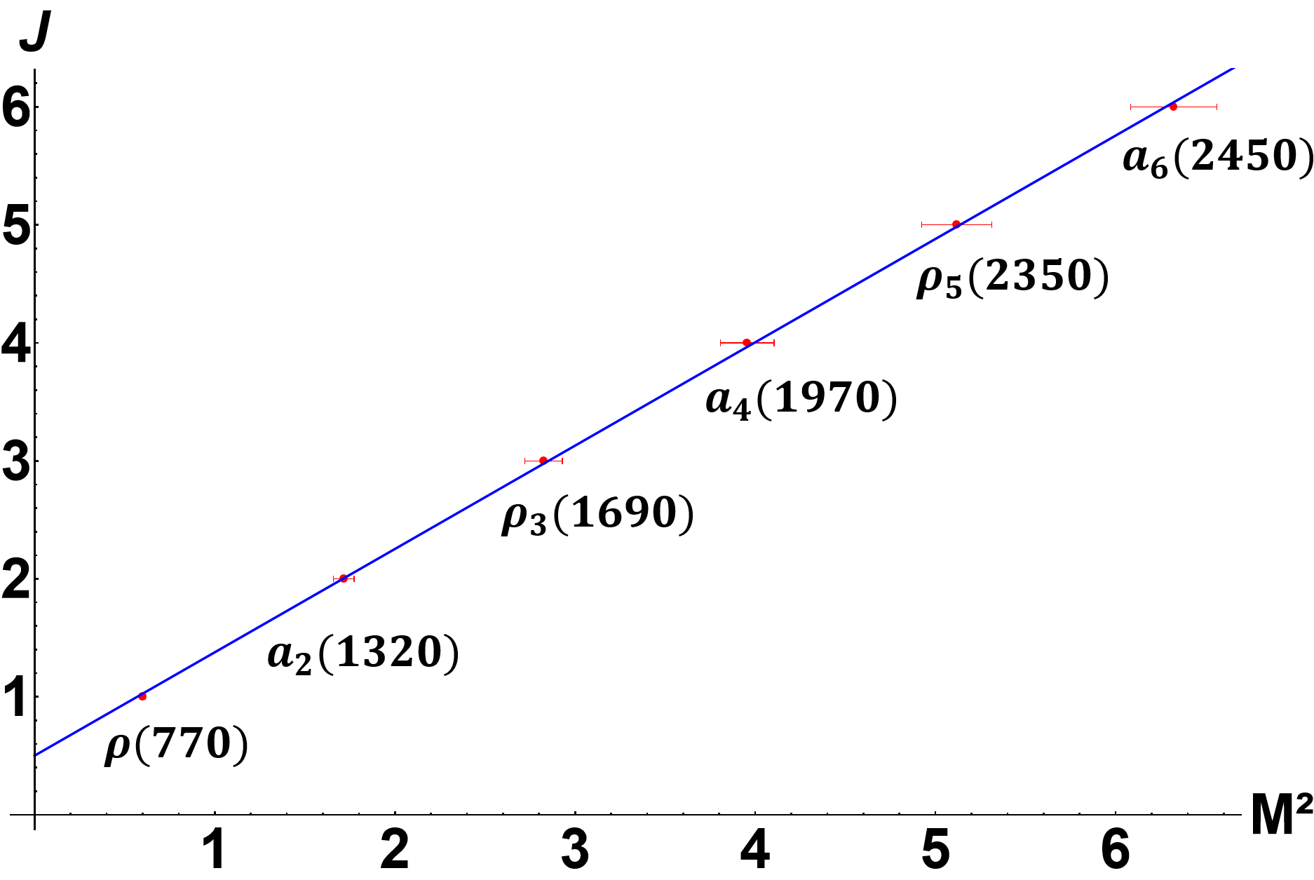
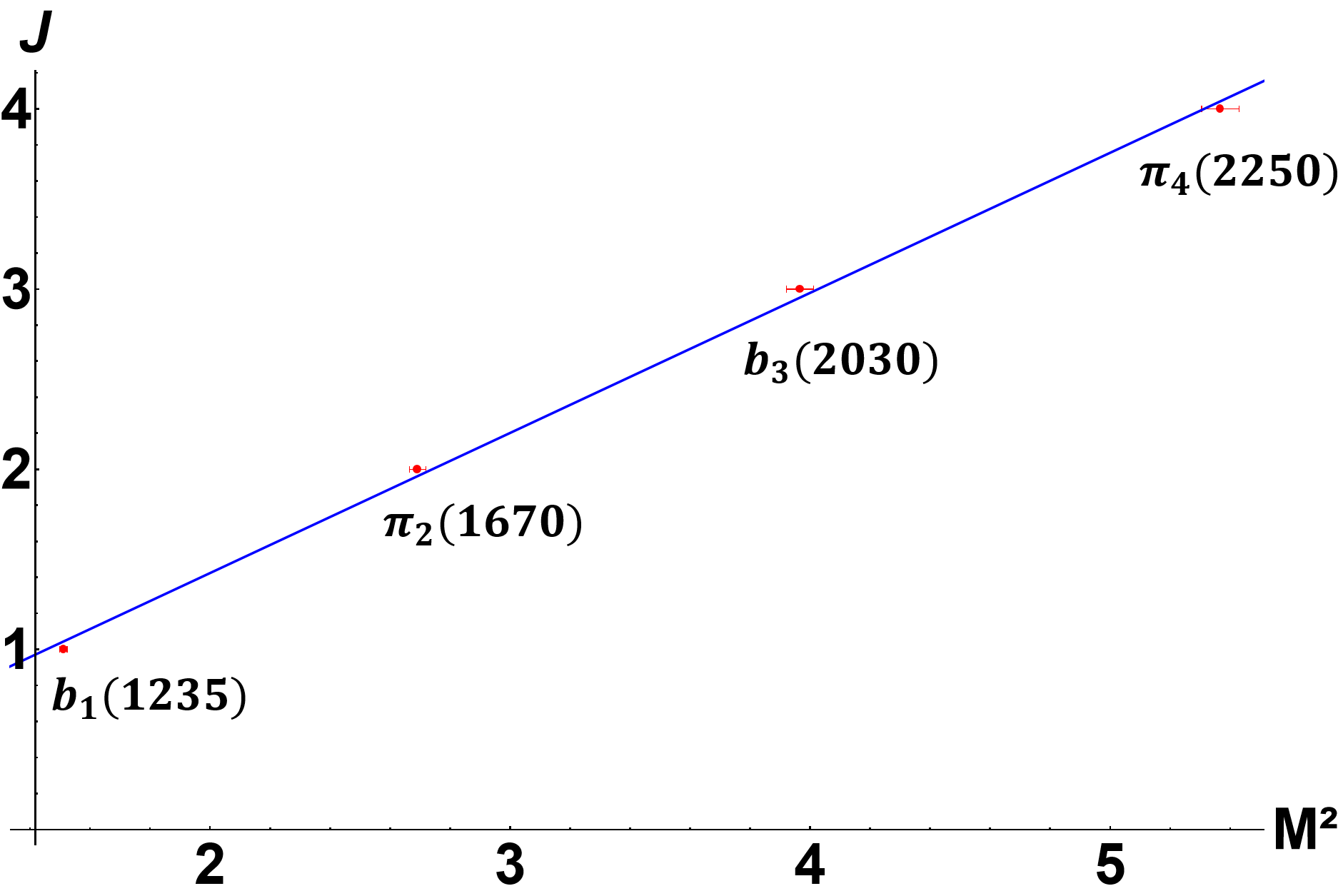
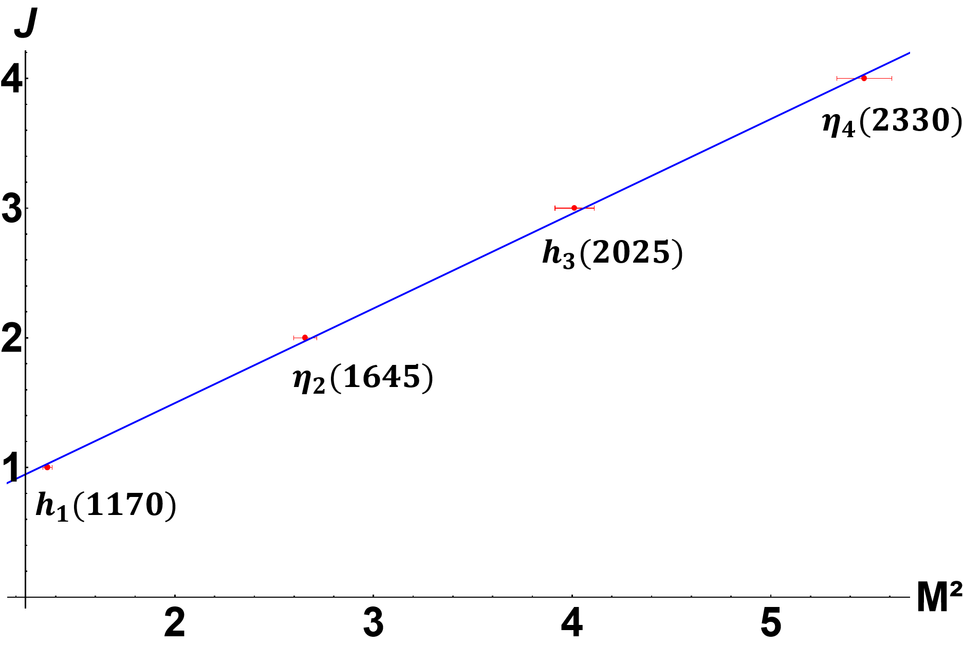
Figure 1: Regge trajectories (blue lines) for mesons, with masses $m$ expressed in GeV, from the AHW Log model. Red dots are the values obtained from Eq. (23) in the AHW Log model with uncertainties shown in Table 3. The blue lines are obtained by linear regression of these points. Upper left panel: mesons with even ${\cal CP}$, $I=1$ ($\rho(770)$ family); Upper right panel: mesons with even ${\cal CP}$, $I=0$ ($\omega(782)$ family); Lower left panel: mesons with odd ${\cal CP}$, $I=1$ ($b_{1}(1235)$ family); Lower right panel: mesons with odd ${\cal CP}$, $I=0$ ($h_{1}(1170)$ family).

III.4 AHW model for mesons with odd ${\cal CP}$, $I=0$, and $S\geq 1$

For mesons with odd ${\cal CP}$, $I=0$, and $S\geq 1$, we minimize the function $Q$, Eq. (25), finding $a=0.95\pm 0.06$ for the anomalous dimension, Eq. (22), obtaining

$$\Delta_{\rm Log}(S)=(0.95\pm 0.06)\ln(S).$$ (33)

The masses obtained in this AHW Log model are presented, with uncertainties, in Table 3, where we used the mass value of the state $h_{1}(1170)$ from PDG as an input, such that $\Lambda_{\rm QCD}=227.04$ MeV. The Regge trajectory obtained by doing linear regression with these masses is given by

$$J=(0.73\pm 0.01)M^{2}+0.04\pm 0.05,$$ (34)

with $\chi^{2}$/ndf$=3.52/2=1.76.$ This trajectory can be compared with the one obtained from PDG data shown in Table 2 and is presented in the lower right panel of Fig. 1 as the blue line. The red dots are the values of the masses obtained within this AHW Log model with their uncertainties.

IV Linear AHW for mesons

Recently, we have shown Costa-Silva:2023vuu that one can obtain asymptotically linear Regge trajectories for glueballs with even spins $S$ from an AHW model, when considering a total dimension $\Delta_{\rm Total}$ proportional to $\sqrt{S}$. In order to find asymptotically linear Regge trajectories for light unflavored mesons with spins $S\geq 1$, we apply a similar procedure here with a small modification in the power of the spins $S$ as

$$\Delta_{\rm Lin}=a_{\rm Lin}(S^{\frac{1}{2}+\epsilon}-1)+4,$$ (35)

where in the ideal case, $\epsilon\rightarrow 0$. Note that when $S=1$, which are the lowest spin state for each mesonic family considered here, we recover the canonical dimension $\Delta=4$, compatible with Eq. (11).

Here, the parameter $a_{\rm Lin}$ is obtained exactly as in the AHW Log model, by minimizing $Q$ in Eq. (25). The parameter $\epsilon$ that represents a little deviation of the ideal case $\epsilon=0$ is chosen to obtain the best asymptotic linear Regge trajectory for each meson family. The value of $\epsilon$ is the one that minimizes the total deviation of the masses from the straight line representing the Regge trajectory.

The masses that follows from this linear AHW model are determined by

$$m_{\nu,1}=\chi_{\nu,1}\Lambda_{\rm QCD};\qquad\qquad(\nu=\Delta_{\rm Lin}-2),$$ (36)

where $\Delta_{\rm Lin}$ is defined in Eq. (35). Since $\Delta_{\rm Lin}=4$ for $S=1$, the values of $\Lambda_{\rm QCD}$ here in this model, for each meson family, are the same as those in the AHW Log model, as well as in the original HW presented in Table 2.

As in the case of logarithmic anomalous dimension, we will analyze the families of light unflavored mesons with even or odd $\cal CP$, isospins $I=0,1$, and spins $S\geq 1$. The Regge trajectories that we obtain within this model are asymptotically linear for each meson family with the appropriate choice of parameters.

IV.1 Linear AHW for mesons with even ${\cal CP}$, $I=1$, and $S\geq 1$

For mesons with even ${\cal CP}$, isospin $I=1$, and spin $S\geq 1$, the parameters in Eq. (35) that minimizes $Q$ are $a_{\rm Lin}=6.87\pm 0.16$ and $\epsilon=0$, so the total dimension reads

$$\Delta_{\rm Lin}=(6.87\pm 0.16)\sqrt{S}-2.87\pm 0.16.$$ (37)

The masses obtained here, using Eq. (36), are presented in Table 4, with respectives uncertainties, using the mass of the state $\rho(770)$ as an input from PDG. The Regge trajectory for these mesons is given by

$$J=(0.87\pm 0.01)M^{2}+0.51\pm 0.02,$$ (38)

with $\chi^{2}$/ndf$=8.68/4=2.17$ and is presented in the upper left panel of Fig. 2 as the blue line. The red dots represent these masses with their uncertainties.

In order to show that the linear AHW model indeed present asymptotic linear Regge trajectories we also plot $J\times M^{2}$ for these mesons with even $\mathcal{CP}$, isospin $I=1$, and $S\geq 1$, for the first 50 states. The trajectory in this case becomes

$$J=(0.8479\pm 0.0002)M^{2}+0.60\pm 0.01,$$ (39)

with $\chi^{2}$/ndf$=72.96/48=1.52.$ This trajectory is presented in the upper left panel of Fig. 3. Both trajectories can be compared with the one obtained from PDG data shown in Table 2 and are in good agreement with it.

Table 4: Masses in MeV for mesons classified under even or odd $\mathcal{CP}$ with isospin $I=0,1$ and spins $S\geq 1$ from the Linear AHW model, determined from Eq. (36), and the percentual deviations $\delta_{\rm Lin}$ of the masses from this model compared with PDG data. For each family the mass of the state with $J=S=1$ is taken as an input. In the last column we show the total dimension $\Delta_{\rm Lin}$ for each state determined by Eq. (35).

$J^{PC}$	$\mathcal{CP}$	I	Meson	Linear AHW	$\delta_{\rm LAHW}$	$\Delta_{\rm Lin}$
$1^{--}$	even	1	$\rho(770)$	$775.26\pm 10.08$	$0\%$	$0$
$2^{++}$	even	1	$a_{2}(1320)$	$1296.75\pm 21$	$1.53\%$	$1.85$
$3^{--}$	even	1	$\rho_{3}(1690)$	$1678.61\pm 30$	$0.60\%$	$3.03$
$4^{++}$	even	1	$a_{4}(1970)$	$1993.84\pm 38$	$1.36\%$	$3.87$
$5^{--}$	even	1	$\rho_{5}(2350)$	$2268.03\pm 44$	$2.66\%$	$4.49$
$6^{++}$	even	1	$a_{6}(2450)$	$2513.71\pm 51$	$2.60\%$	$4.96$
$1^{--}$	even	0	$\omega(782)$	$782.66\pm 7.83$	$0\%$	$0$
$2^{++}$	even	0	$f_{2}(1270)$	$1294.28\pm 16$	$1.47\%$	$1.76$
$3^{--}$	even	0	$\omega_{3}(1670)$	$1669.09\pm 22$	$0.13\%$	$2.88$
$4^{++}$	even	0	$f_{4}(2050)$	$1978.53\pm 28$	$1.96\%$	$3.67$
$5^{--}$	even	0	$\omega_{5}(2250)$	$2247.67\pm 33$	$0.10\%$	$4.24$
$6^{++}$	even	0	$f_{6}(2510)$	$2488.81\pm 38$	$0.97\%$	$4.67$
$1^{+-}$	odd	1	$b_{1}(1235)$	$1229.5\pm 5.0$	$0\%$	$0$
$2^{-+}$	odd	1	$\pi_{2}(1670)$	$1667.30\pm 7.89$	$0.20\%$	$0.48$
$3^{+-}$	odd	1	$b_{3}(2030)$	$2000.60\pm 10.75$	$1.55\%$	$0.65$
$4^{-+}$	odd	1	$\pi_{4}(2250)$	$2281.03\pm 13.31$	$1.38\%$	$0.65$
$1^{+-}$	odd	0	$h_{1}(1170)$	$1166\pm 10$	$0\%$	$0$
$2^{-+}$	odd	0	$\eta_{2}(1645)$	$1646.87\pm 17$	$1.85\%$	$0.72$
$3^{+-}$	odd	0	$h_{3}(2025)$	$2009.96\pm 24$	$0.74\%$	$1.07$
$4^{-+}$	odd	0	$\eta_{4}(2330)$	$2314.19\pm 31$	$0.59\%$	$1.22$

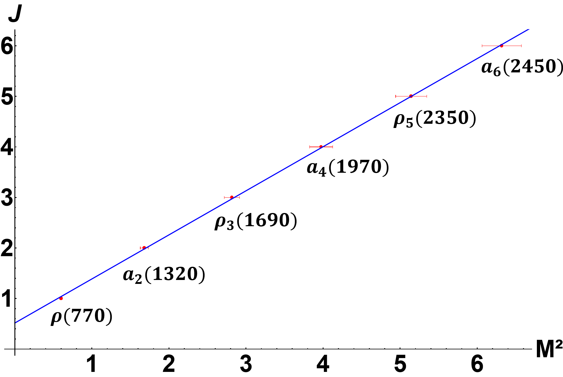
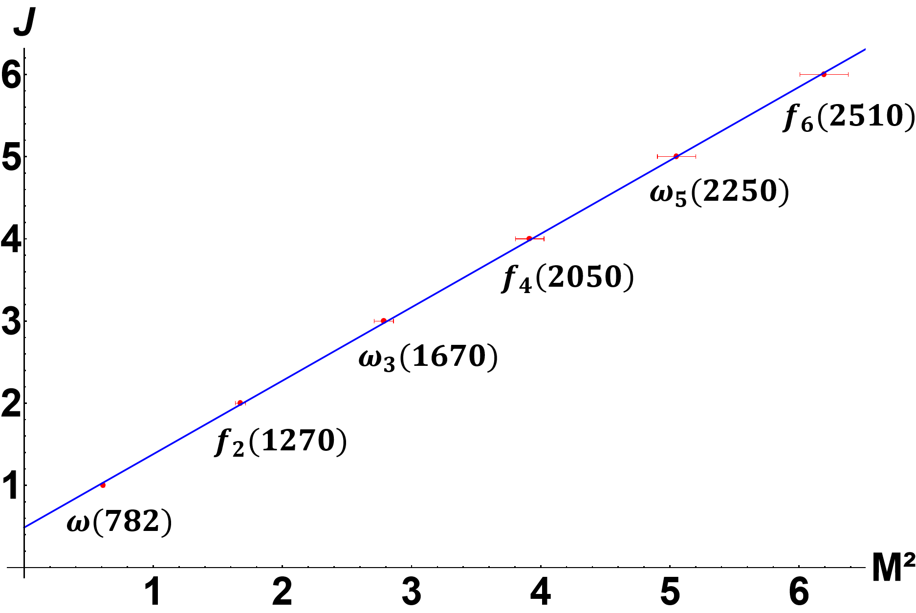
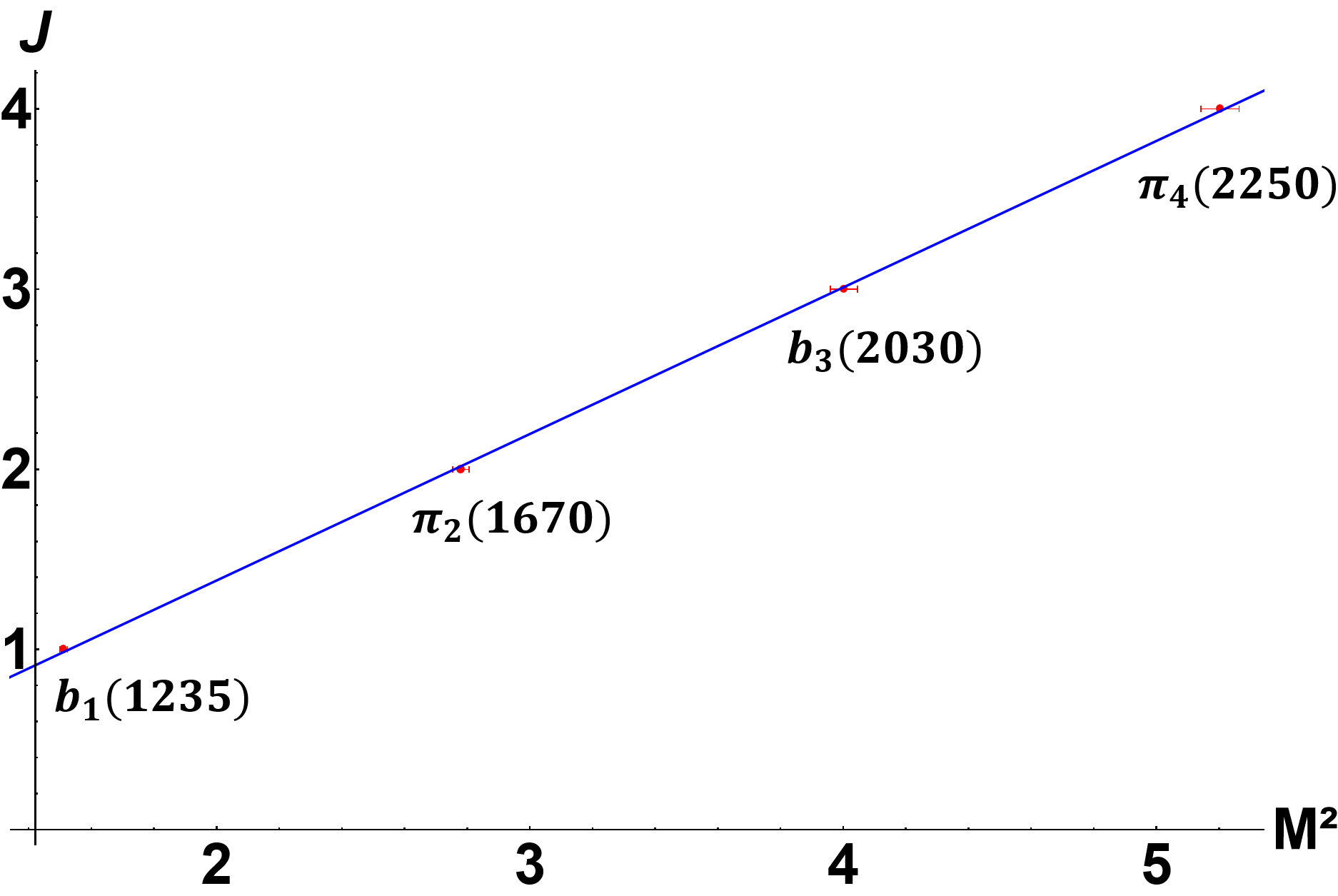
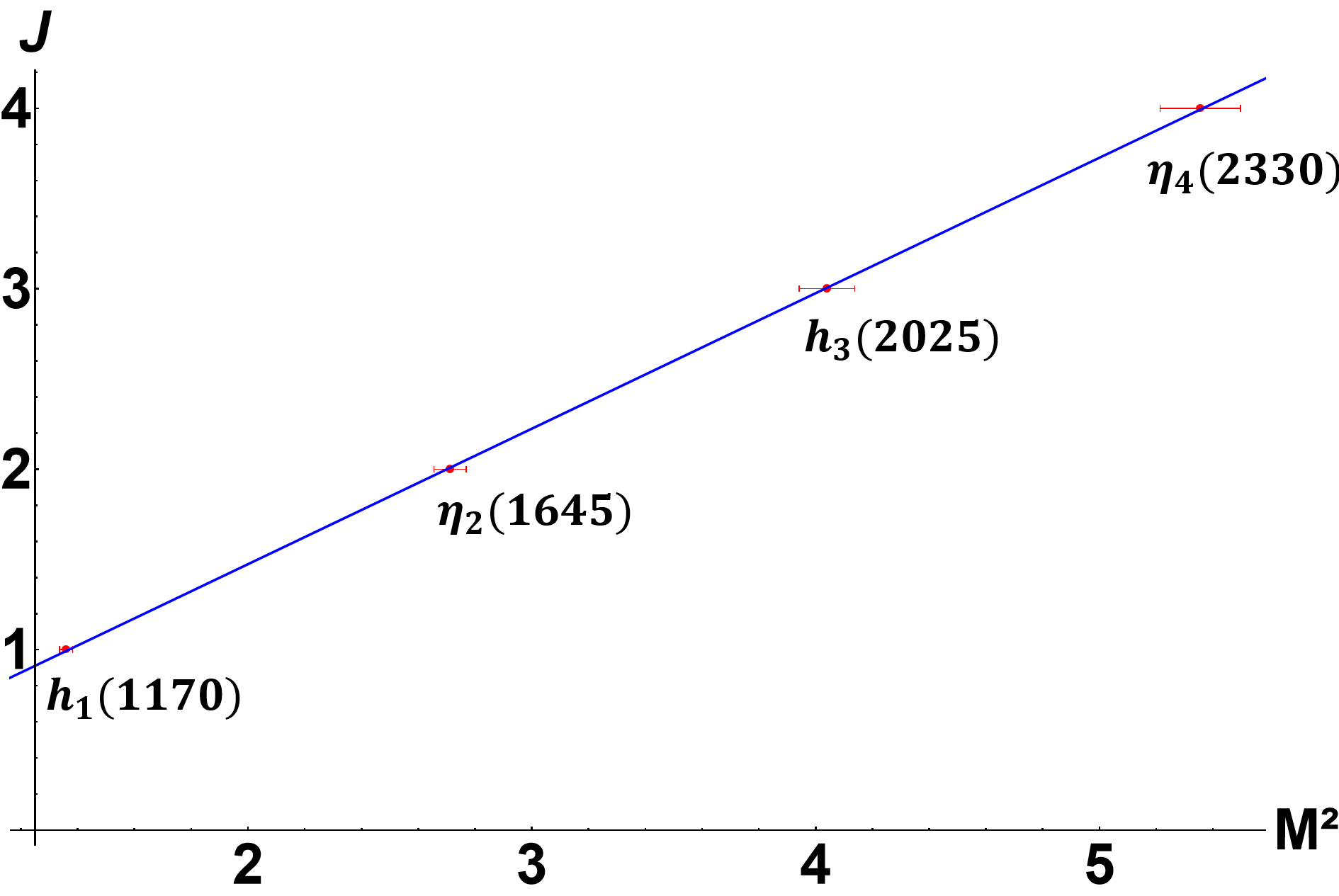
Figure 2: Regge trajectories (blue lines) for mesons, with masses $m$ expressed in GeV, from the Linear AHW model, with total dimension given by Eq. (35). Red dots are the values obtained from Eq. (36) with uncertainties and the blue lines are obtained by linear regression of these points, for each meson family. Upper left panel: mesons with even ${\cal CP}$, $I=1$ ($\rho(770)$ family); Upper right panel: mesons with even ${\cal CP}$, $I=0$ ($\omega(782)$ family); Lower left panel: mesons with odd ${\cal CP}$, $I=1$ ($b_{1}(1235)$ family); Lower right panel: mesons with odd ${\cal CP}$, $I=0$ ($h_{1}(1170)$ family).

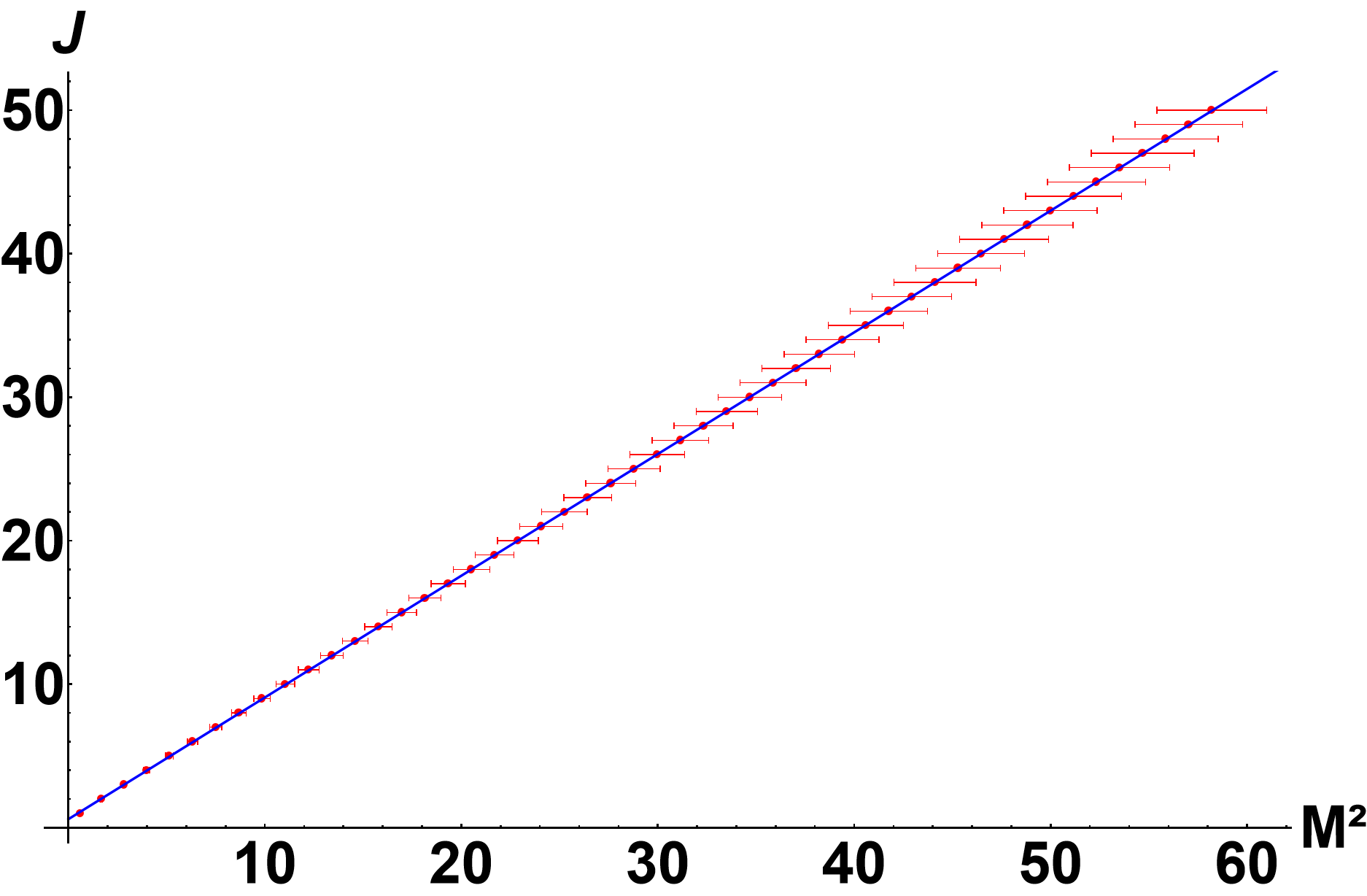
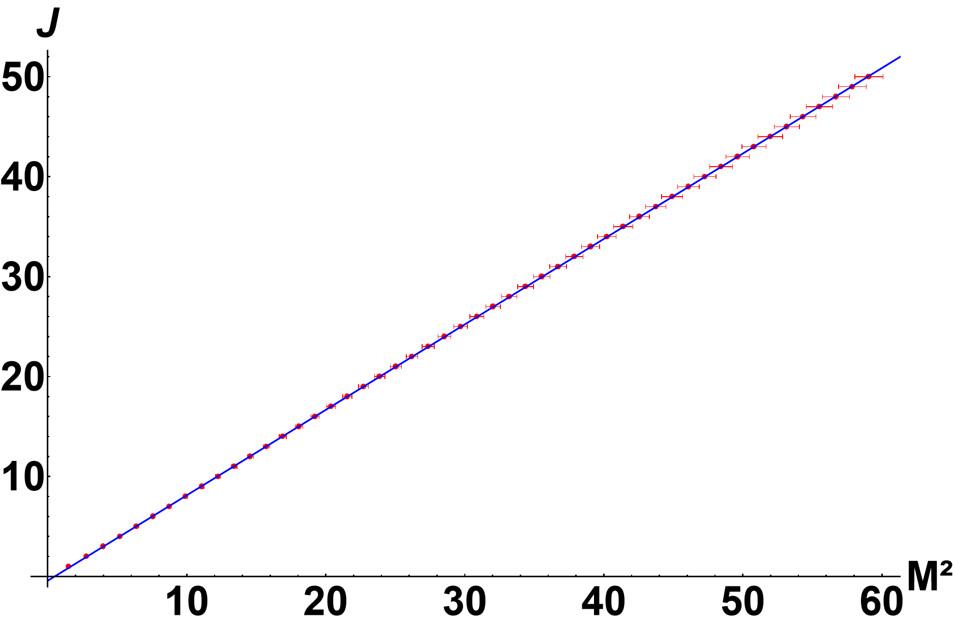
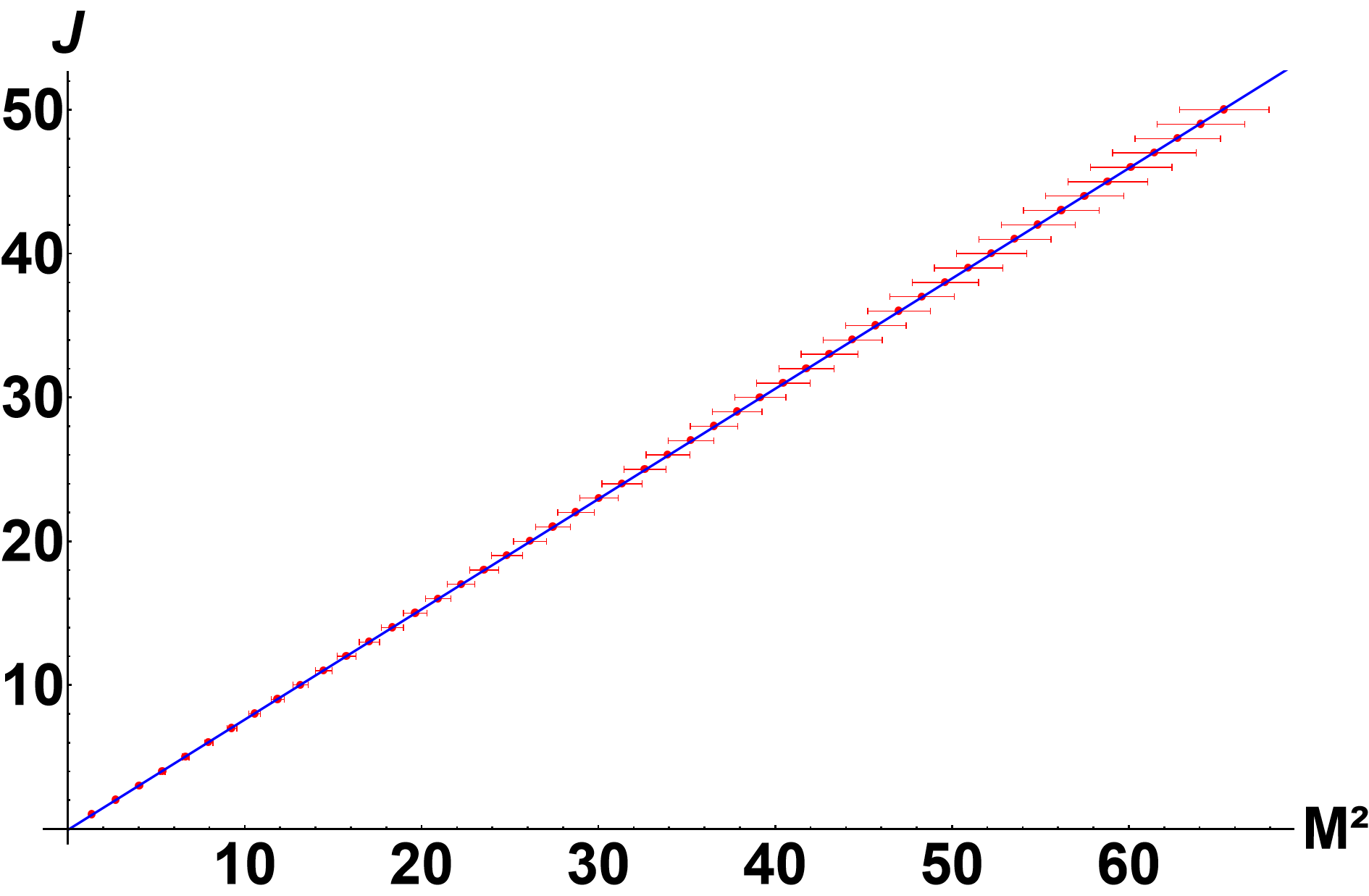
Figure 3: Regge trajectories for mesons, with masses $m$ expressed in GeV, from the linear AHW model, with total dimension given by Eq. (35). Red dots are the values obtained from Eq. (36) with uncertainties and the blue lines are the Regge trajectories, obtained by linear regression of these 50 points, for each meson family. Upper left panel: mesons with even ${\cal CP}$, $I=1$ ($\rho(770)$ family); Upper right panel: mesons with even ${\cal CP}$, $I=0$ ($\omega(782)$ family); Lower left panel: mesons with odd ${\cal CP}$, $I=1$ ($b_{1}(1235)$ family); Lower right panel: mesons with odd ${\cal CP}$, $I=0$ ($h_{1}(1170)$ family).

IV.2 Linear AHW for mesons with even ${\cal CP}$, $I=0$, and $S\geq 1$

For mesons in the linear AHW model with even ${\cal CP}$, $I=1$, and $S\geq 1$, the parameters in Eq. (35) that minimizes $Q$ are $a_{\rm Lin}=6.67\pm 0.13$ and $\epsilon=0$. So, the total dimension reads

$$\Delta_{\rm Lin}=(6.67\pm 0.13)\sqrt{S}-2.67\pm 0.13.$$ (40)

The masses obtained by this model, using Eq. (36), are presented with respectives uncertainties in Table 4, taking the mass of the state $\omega(782)$ as an input from PDG. Furthermore, we also present in this table the total dimension and the percentual deviations from PDG data for each mesonic state. The Regge trajectory obtained by linear regression of these masses (first six states) is presented in the upper right panel of Fig. 2 and is given by

$$J=(0.89\pm 0.01)M^{2}+0.49\pm 0.02,$$ (41)

with $\chi^{2}$/ndf$=10.12/4=2.53.$ The upper right panel of Fig. 3 presents the Regge trajectory for the first 50 sates with even ${\cal CP}$, $I=0$, and $S\geq 1$, and it is given by

$$J=(0.8766\pm 0.0003)M^{2}+0.52\pm 0.01,$$ (42)

with $\chi^{2}$/ndf$=32.16/48=0.67.$ Both equations can be compared with the one obtained from PDG data, shown in Table 2, and are in good agreement with it.

IV.3 Linear AHW for mesons with odd ${\cal CP}$, $I=1$, and $S\geq 1$

For mesons with odd ${\cal CP}$, $I=1$, and $S\geq 1$ ($b_{1}(1235)$ family), the parameters in Eq. (35) that minimizes $Q$ are $a_{\rm Lin}=3.19\pm 0.03$ and $\epsilon=0.05$, so the total dimension becomes

$$\Delta_{\rm Lin}=(3.19\pm 0.03)S^{0.55}+0.81\pm 0.03.$$ (43)

The masses obtained in this model, using Eq. (36), are presented in Table 4. The Regge trajectory obtained for the first four points is presented in Fig. 2 and is given by

$$J=(0.81\pm 0.01)M^{2}-0.24\pm 0.03,$$ (44)

with $\chi^{2}$/ndf$=2.86/2=1.43.$

For 50 points the trajectory is in Fig. 3 and is given by

$$J=(0.8549\pm 0.0003)M^{2}-0.42\pm 0.01,$$ (45)

with $\chi^{2}$/ndf$=163/48=3.39.$ Both equations, considering the uncertainties, are in agreement with the Regge trajectory obtained from PDG data, shown in Table 2.

IV.4 Linear AHW for mesons with odd ${\cal CP}$, $I=0$, and $S\geq 1$

The parameters in Eq. (35) that minimizes $Q$ for meson with mesons with odd ${\cal CP}$, $I=0$, and $S\geq 1$ ($h_{1}(1170)$ family) are $a_{\rm Lin}=3.79\pm 0.08$ and $\epsilon=0.04$, so the total dimension is

$$\Delta_{\rm Lin}=(3.79\pm 0.08)S^{0.54}+0.21\pm 0.08.$$ (46)

The masses obtained in this model, using Eq. (36), are presented in Table 4. The Regge trajectory for the first four points is presented in Fig. 2 and is

$$J=(0.7509\pm 0.033)M^{2}-0.03\pm 0.01,$$ (47)

with $\chi^{2}$/ndf$=0.22/2=0.11.$ The Fig. 3 presents the Regge trajectory for the first 50 points, given by

$$J=(0.7667\pm 0.0003)M^{2}-0.06\pm 0.01,$$ (48)

with $\chi^{2}$/ndf$=2.20/48=0.046.$ Both trajectories are in good agreement the one from PDG shown in Table 2.

V Conclusions

In this work, we proposed anomalous and linear HW models for light unflavored mesons. We have shown that the masses and Regge trajectories produced by these models are better than that obtained from the original HW and SW models.

In particular, the linear AHW model produce asymptotically linear Regge trajectories, circumventing the well-kown problem of non-linearity of the original HW model.

Finally, we expect to succesfully extend the analysis presented here to other particles as heavy and heavy-light mesons, as well as baryons. This is presently under investigation.

References

O. Aharony, S. S. Gubser, J. M. Maldacena, H. Ooguri and Y. Oz, “Large N field theories, string theory and gravity,” Phys. Rept. 323, 183-386 (2000) doi:10.1016/S0370-1573(99)00083-6 [arXiv:hep-th/9905111 [hep-th]].

J. Casalderrey-Solana, H. Liu, D. Mateos, K. Rajagopal and U. A. Wiedemann, “Gauge/String Duality, Hot QCD and Heavy Ion Collisions,” Cambridge University Press, 2014, doi:10.1017/9781009403504 [arXiv:1101.0618 [hep-th]].

J. Zaanen, Y. W. Sun, Y. Liu and K. Schalm, “Holographic Duality in Condensed Matter Physics,” Cambridge Univ. Press, 2015, doi:10.1017/CBO9781139942492

H. Boschi-Filho and N. R. F. Braga, “Gauge / string duality and scalar glueball mass ratios,” JHEP 05, 009 (2003) doi:10.1088/1126-6708/2003/05/009 [arXiv:hep-th/0212207 [hep-th]].

H. Boschi-Filho and N. R. F. Braga, “QCD / string holographic mapping and glueball mass spectrum,” Eur. Phys. J. C 32, 529-533 (2004) doi:10.1140/epjc/s2003-01526-4 [arXiv:hep-th/0209080 [hep-th]].

G. F. de Teramond and S. J. Brodsky, “Hadronic spectrum of a holographic dual of QCD,” Phys. Rev. Lett. 94, 201601 (2005) doi:10.1103/PhysRevLett.94.201601 [arXiv:hep-th/0501022 [hep-th]].

J. Erlich, E. Katz, D. T. Son and M. A. Stephanov, “QCD and a holographic model of hadrons,” Phys. Rev. Lett. 95, 261602 (2005) doi:10.1103/PhysRevLett.95.261602 [arXiv:hep-ph/0501128 [hep-ph]].

H. Boschi-Filho, N. R. F. Braga and H. L. Carrion, “Glueball Regge trajectories from gauge/string duality and the Pomeron,” Phys. Rev. D 73, 047901 (2006) doi:10.1103/PhysRevD.73.047901 [arXiv:hep-th/0507063 [hep-th]].

A. Karch, E. Katz, D. T. Son and M. A. Stephanov, “Linear confinement and AdS/QCD,” Phys. Rev. D 74, 015005 (2006) doi:10.1103/PhysRevD.74.015005 [arXiv:hep-ph/0602229 [hep-ph]].

P. Colangelo, F. De Fazio, F. Giannuzzi, F. Jugeau and S. Nicotri, “Light scalar mesons in the soft-wall model of AdS/QCD,” Phys. Rev. D 78, 055009 (2008) doi:10.1103/PhysRevD.78.055009 [arXiv:0807.1054 [hep-ph]].

S. S. Gubser, I. R. Klebanov and A. M. Polyakov, “A Semiclassical limit of the gauge / string correspondence,” Nucl. Phys. B 636, 99-114 (2002) doi:10.1016/S0550-3213(02)00373-5 [arXiv:hep-th/0204051 [hep-th]].

R. A. Costa-Silva and H. Boschi-Filho, “Anomalous and linear holographic hard wall models for glueballs and the pomeron,” Phys. Rev. D 109, no.8, 086019 (2024) doi:10.1103/PhysRevD.109.086019 [arXiv:2306.04728 [hep-ph]].

R. L. Workman et al. [Particle Data Group], “Review of Particle Physics,” PTEP 2022, 083C01 (2022) doi:10.1093/ptep/ptac097

J. K. Chen, “Structure of the meson Regge trajectories,” Eur. Phys. J. A 57, no.7, 238 (2021) doi:10.1140/epja/s10050-021-00502-y [arXiv:2102.07993 [hep-ph]].