Metaheuristic Approaches to the Placement of Suicide Bomber Detectors

Abstract

Suicide bombing is an infamous form of terrorism that is becoming increasingly prevalent in the current era of global terror warfare. We consider the case of targeted attacks of this kind, and the use of detectors distributed over the area under threat as a protective countermeasure. Such detectors are non-fully reliable, and must be strategically placed in order to maximize the chances of detecting the attack, hence minimizing the expected number of casualties. To this end, different metaheuristic approaches based on local search and on population-based search are considered and benchmarked against a powerful greedy heuristic from the literature. We conduct an extensive empirical evaluation on synthetic instances featuring very diverse properties. Most metaheuristics outperform the greedy algorithm, and a hill-climber is shown to be superior to remaining approaches. This hill-climber is subsequently subject to a sensitivity analysis to determine which problem features make it stand above the greedy approach, and is finally deployed on a number of problem instances built after realistic scenarios, corroborating the good performance of the heuristic.

1 Introduction

At the time of writing this paper, the Atatürk Airport in Istanbul was subject to a terrorist attack whose perpetrators carried automatic weapons and explosive belts. As a result of the shooting and the detonation of the suicide bombs, 44 people were killed (in addition to the three terrorists) and more than 200 were injured (Kurukiz, 2016). A few days afterwards, a suicide car bombing killed 292 people and left more than 200 people wounded in a shopping district of Baghdad, in what constituted the deadliest single bomb attack in Iraq since 2007 (AFP, 2016). These are only two recent examples of suicide bombings, a form of terrorism that not only causes about four time more casualties than other kinds of terrorist attack (Rand Corporation, 2009), cf. (Hoffman, 2003) but also instills a sense of fear in the society as a whole that undermines public confidence in the authorities and contributes to subjugate those living under this threat (Hoffman, 2003). As a result of the relative inexpensiveness (they do not require escaping logistics nor sophisticated equipment for remote operation) and effectiveness of this kind of attacks, they have become increasingly prevalent; see Figure 1. Indeed, they are not just very frequent in conflicting areas such as the Middle East –1,192 attacks in the period 1982-2015, only counting those conducted using explosive belts (Chicago Project on Security and Terrorism (2016), CPOST)– but also constitute a global threat that has caused nearly 50,000 deaths worldwide in the 21st Century, with an average of about 10 fatalities and 24 non-fatal casualties per attack (counting all suicide attacks – data from Chicago Project on Security and Terrorism (2016) (CPOST)).

In response to this ongoing threat, security forces and intelligence agencies are strengthening their efforts. Obviously, the nature of this kind of attack makes it infeasible to rely on standard deterrence measures based on direct retaliation. Hence, other members of the terrorist network providing intellectual or logistic support to the attacker (and in general any assets valued by the latter) are targeted instead (Kroenig and Pavel, 2012). In any case, this does not fully deters this kind of attacks, so they must be also fought against by trying to deny their benefits, either at a strategic level (ensuring that the ultimate goals of the terrorists will not be achieved even if the attack was successful) or at a tactical level (trying to make the attacks unsuccessful). Heightened security measures in airports, government buildings or military installations are examples of this latter kind of counterterrorism measures.

Figure 1: The bart chart shows the number of casualties (dead and injured) in suicide attacks in the period 2001-2015 (total year figures on top of each bar, scale on the left). The black curve indicates the number of suicide attacks in this time frame (scale on the right). Source: own elaboration based on data from (Chicago Project on Security and Terrorism (2016), CPOST).

A potential problem of these explicit, partly invasive security measures is that they cannot be readily exported to other kind of environments also susceptible to terror attacks (e.g., placing airport-like scanners surrounding a city square or busy shopping street, or frisking every passer-by is out of question). More subtle surveillance can be accomplished by using chemical or biological sensors tailored to detect traces of explosives in their proximity (NRC, 2004; Singh, 2007; Yinon, 2007; Caygill et al, 2012). In this sense, Kaplan and Kress (2005) studied the deployment of such sensors in urban areas subject to pedestrian suicide-bombing attacks. They analyzed different scenarios (an urban grid of streets and a large plaza or park) and concluded that, while such sensors are not likely effective against random attacks, they can play an important role in the defense of known targets. Building on this work, Nie et al (2007) considered the case of a threat area with known targets on which a number of non-fully reliable sensors are deployed. They proposed a branch-and-bound algorithm (BnB) and a greedy constructive heuristic to determine the location of these sensors so as to minimize the casualties. The BnB algorithm does not scale well with problem size, but the greedy heuristic is relatively effective (although it will not guarantee finding the optimal solution in general).

Following these previous results, the problem is here approached for the first time to the best of our knowledge from the point of view of iterative heuristics and metaheuristic techniques. We propose several algorithms based on local search, greedy randomized adaptive search procedures and evolutionary algorithms, and analyze their performance, comparing it to the greedy approach previously mentioned on an extensive collection of synthetic and real scenarios. Before presenting the algorithms considered and the experimental setup, let us firstly define formally the problem tackled. This is done in next section.

2 Problem Description

Let us assume the goal is to protect a certain threat area or scenario which we can model as a rectangular grid ${A}=\{A_{ij}\}_{m\times n}$. Each cell in this grid represents a small square subarea which can be blocked if there is some physical obstruction (a wall, a monument, etc.) that precludes its being traversed by the attacker, or unblocked if it can be freely accessed. Some of these latter unblocked cells can be also objectives, that is, cells that contain threatened individuals who may be targeted by the attacker. To carry on this threat, the attacker can enter the scenario through some entrances, namely specific unblocked cells typically placed in the boundaries of the grid. From any of those entrances, the attacker will try to reach any of the objectives following always a shortest path. Following (Nie et al, 2007), the attacker is able to move in a straight line from the center of a grid cell to the center of any other one for which this line does not intersect with a blocked cell. Thus, the path followed by the attacker will be composed by a number of straight segments, and can be computed by running classical algorithms –such as, e.g., Dijkstra’s algorithm or A*– on a weighted complete graph $G(V,E,w)$, where

• $V=\{\langle i,j\rangle\ |\ A_{ij}$ is unblocked$\}$, i.e., a vertex per unblocked cell,

• $E=V\times V$, and

• $w:E\rightarrow\mathbb{R}$ is defined as

  $$w((\langle i_{1},j_{1}\rangle,\langle i_{2},j_{2}\rangle))=\zeta\sqrt{(i_{1}-i_{2})^{2}+(j_{1}-j_{2})^{2}},$$ (1)

  (where $\zeta$ is the side of each grid cell) if there is no obstacle in the straight path among both cells, and $w(E)=\infty$ otherwise.

Figure 2 shows an example $8\times 8$ scenario with 8 entrances, 6 blocked cells and 2 objectives. Notice how paths try to follow always a straight line towards the objective, taking small detours if there are obstacles on the way.

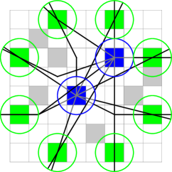
Figure 2: An $8\times 8$ scenario. Green cells correspond to entrances, blue ones to objectives and gray cells represent blocked locations. Lines are shortest paths from each entrance to each objective (note that paths would be extended backwards should a detector be placed on any of the entrances). The dimension of each cell is 10m $\times$ 10m, and the attacker must be neutralized at least 10m away from an objective (we assume that the terrorist moves at a speed of 1m/s and that aborting the attack requires no more than 10 seconds).

With this setting in mind, the problem under consideration amounts to placing some detectors in different unblocked cells of the grid. These detectors are perfectly concealed from the attacker, but they are not fully reliable and will only detect attackers that travel within a certain detection radius $\tau$ of the detector with a probability $p$ that depends on the length of the attacker’s path inside this detection area (a circle of radius $\tau$ centered in the detector’s location). Detection does not imply neutralization of the attacker though. It only amounts to firing some alarm that elicits response from some enforcing agents, and that can lead to effective negation of the attack only if the attacker is not yet very close to the objective, and with some probability $\theta$. Let us formalize the whole process in the following.

Let $\varepsilon$ and $\phi$ be the number of entrances and objectives respectively. For each entrance $e_{i}$, $1\leqslant i\leqslant\varepsilon$, and objective $o_{j}$, $1\leqslant j\leqslant\phi$ there is a path $P_{ij}$ (we assume for simplicity that the shortest path is unique – considering multiple paths does not fundamentally affect the analysis below). The attacker will pick an entrance $e_{i}$ and an objective $o_{j}$ with probability $\gamma_{ij}$ (obviously, $\sum_{i=1}^{\varepsilon}\sum_{j=1}^{\phi}\gamma_{ij}=1$) and will subsequently move along $P_{ij}$ at speed $v$. Neutralizing the attack once detected takes some time $t_{n}$ –at least 10s according to Kaplan and Kress (2005)– and hence once the attacker is at distance $vt_{n}$ from the objective (distance measured along the path $P_{ij}$) no effective neutralization is possible. Therefore, let us define $\bar{P}_{ij}$ as the portion of the path $P_{ij}$ outside this “dead” zone, in which timely detection is still possible.

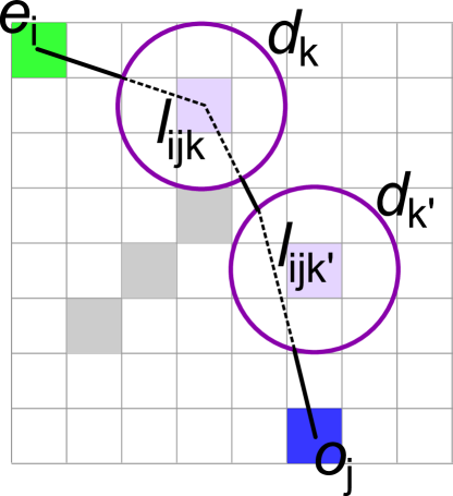
Figure 3: A shortest path going from entrance $e_{i}$ to objective $o_{j}$. Areas monitored by detectors $d_{k}$ and $d_{k}^{\prime}$ are those enclosed by circumferences. The segments of this path detected by both detectors are shown with a dotted line and denoted by $l_{ijk}$ and $l_{ijk^{\prime}}$.

Now, let $\delta$ be the number of detectors in the scenario. A certain detector $d_{k}$, $1\leqslant k\leqslant\delta$, will timely detect an attacker traveling through $P_{ij}$ with probability

$$p_{ijk}=1-\exp(-\eta l_{ijk})$$ (2)

where $l_{ijk}$ is the length of the segment of $\bar{P}_{ij}$ within the circle of radius $\tau$ centered at $d_{k}$, and $\eta>0$ is a parameter (the detector’s instantaneous detection rate). It follows that the larger this segment, the larger the detection probability (and obviously $p_{ijk}=0$ if $l_{ijk}=0$, i.e., if the path is outside the detection radius of $d_{k}$) – see Figure 3 for an example. Following (Nie et al, 2007), detectors are assumed to work independently of one another, and therefore the total probability of non-detection $\tilde{D}_{ij}$ if the attacker follows $P_{ij}$ is

$$\tilde{D}_{ij}=\prod_{k=1}^{\delta}(1-p_{ijk})=\prod_{k=1}^{\delta}\exp(-\eta l_{ijk})=\exp(-\eta\sum_{k=1}^{\delta}l_{ijk})$$ (3)

In case of non-detection, the attacker will reach the objective $o_{j}$ causing a number of casualties $C_{j}$. This will be also the case, should the attacker be timely detected but not effectively neutralized (an event that will happen with probability $1-\theta$). The expected number of casualties $W_{ij}$ for this particular path will thus be

$$W_{ij}=\tilde{D}_{ij}C_{j}+(1-\tilde{D}_{ij})(1-\theta)C_{j}=C_{j}\left[\tilde{D}_{ij}\theta+(1-\theta)\right]$$ (4)

The total number of casualties will take into account all possible paths $P_{ij}$ the attacker can take, that is, between any entrance $e_{i}$ and objective $o_{j}$ (and recall each of these is picked with probability $\gamma_{ij}$):

$$W = \sum_{i=1}^{\varepsilon}\sum_{j=1}^{\phi}\gamma_{ij}W_{ij}=\sum_{i=1}^{\varepsilon}\sum_{j=1}^{\phi}\gamma_{ij}C_{j}\left[\tilde{D}_{ij}\theta+(1-\theta)\right]=$$ (5)

$$= \sum_{i=1}^{\varepsilon}\sum_{j=1}^{\phi}\gamma_{ij}C_{j}(1-\theta)+\sum_{i=1}^{\varepsilon}\sum_{j=1}^{\phi}\gamma_{ij}C_{j}\tilde{D}_{ij}\theta=$$ (6)

$$= (1-\theta)\sum_{i=1}^{\varepsilon}\sum_{j=1}^{\phi}\gamma_{ij}C_{j}+\theta\sum_{i=1}^{\varepsilon}\sum_{j=1}^{\phi}\gamma_{ij}C_{j}\exp(-\eta\sum_{k=1}^{\delta}l_{ijk})$$ (7)

The objective of the problem is thus placing $\delta$ detectors on the grid such that Equation (7) is minimized (this actually implies minimizing the second term therein since the first one is independent of the placement of the detectors). We shall denote this problem as the Optimal Placement of Suicide-Bomber Detectors (OPSBD).

3 Description of Algorithms

In this section, we describe the different algorithms for the OPSBD problem that we have considered in this work. To this end, we shall start by presenting some general algorithmic considerations that are applicable to all algorithms considered, namely a cache data structure aimed to avoid recomputation and a dominance criterion that reduces the search space. Subsequently, we will provide a detailed description of all heuristics, namely a Greedy Randomized Adaptive Search Procedure (GRASP), a Hill Climber (HC), an Evolutionary Algorithm (EA) and a Univariate Marginal Distribution Algorithm (UMDA). Prior to these and for the sake of completeness, we will also describe the Greedy algorithm proposed by Nie et al (2007), which will be used to benchmark the remaining procedures.

3.1 General Algorithmic Considerations

All algorithms compared in this work use a cache data structure in order to accelerate the otherwise repetitive computations needed during the optimization of a particular instance.

This memory consists of several components. The first one is a three-dimensional array ${\Lambda}=\{\Lambda_{ijp}\}_{m\times n\times r}$ whose first two dimensions correspond to the number of rows ($m$) and columns ($n$) of the map. The third one corresponds to the total number of paths going from each entrance in the map to each objective ($r=\varepsilon\phi$). Each entry in this data structure stores the length of the segment of the path that would be detected by placing a detector at the center of the cell denoted by the two first dimensions, i.e., if detector $d_{k}$ is placed at cell $(i^{\prime},j^{\prime})$, $\Lambda_{i^{\prime}j^{\prime}p}=l_{ijk}$, where $P_{ij}$ is the $p$th path under a certain predefined order and $l_{ijk}$ is as defined in previous section.

Another component of the cache is a bi-dimensional array ${\Delta}=\{\Delta_{ij}\}_{m\times n}$, which stores the number of times each cell in the map is dominated by remaining cells. We say that a cell $c_{1}=(i_{1},j_{1})$ is dominated by another cell $c_{2}=(i_{2},j_{2})$ if,

$$\forall p\in{1,\dots\varepsilon\phi}:\quad \Lambda_{i_{1}j_{1}p}\leqslant\Lambda_{i_{2}j_{2}p}$$ (8)

$$\exists p\in{1,\dots\varepsilon\phi}:\quad \Lambda_{i_{1}j_{1}p}<\Lambda_{i_{2}j_{2}p}$$ (9)

that is, for all paths in the map, the length of the segment of that path that would be detected by placing a detector at cell $c_{1}$ is less than or equal to the one detected by placing instead the detector at cell $c_{2}$, and, for at least one path, the path detected by a detector at $c_{1}$ is strictly less than that detected from $c_{2}$. This concept of dominance can be used to prune the search space of the problem since those cells that are dominated by a number of cells greater than or equal to the total number of detectors to be placed at the map (i.e., $\Delta_{ij}\geqslant\delta$) can be pruned, since there exists at least $\delta$  cells better than those. Figure 4 illustrates dominance values for the scenario shown before.

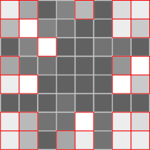
Figure 4: Dominated cells in the map from Figure 2, assuming that a total of $\delta=3$ detectors are to be placed. The detector effectiveness radius is $\tau=10$m. Red bordered cells can be safely disregarded as candidate locations for placing the detectors. Lightest cells are more dominated than darker ones.

3.2 Greedy Algorithm

As mentioned above, this algorithm (denoted as Greedy henceforth) corresponds to the one originally described in (Nie et al, 2007) and will be used to establish a baseline for comparison purposes. This greedy heuristic is a constructive method that places the $\delta$ detectors one at a time as depicted in the pseudo-code provided in Algorithm 1.

Firstly, the set of candidate detectors is initialized with all non-blocked cells in the map minus those that are dominated by at least $\delta$ cells (line 1). The algorithm starts from an empty solution (line 2) and from there on, the $\delta$ detectors are successively added to the current partial solution $\mathit{sol}$ (lines 3-15). In each iteration, the candidate detector whose incorporation leads to the best extended solution –i.e., locally minimizing Equation (7)– is selected (lines 6-12), added to current solution (line 13) and removed from the set of candidate detectors (line 14).

As it can be seen, this greedy algorithm performs different locally optimal decisions which can be taken with a low computational cost. However, due to the myopic functioning of this scheme, the resulting final solution is not guaranteed to be optimal. Although it was shown in (Nie et al, 2007) that the quality of solutions provided by the greedy algorithm for this particular problem is not very far from the global optimum for the relatively small-sized instances that were considered in that work, it will be later shown in Section 4 that other heuristics can provide better solutions for this problem if larger instances are considered.

Input: $\delta$ (number of detectors to be placed)

1 $\mathit{candidates}:=\{(r,c)\ |\ 1\leqslant r\leqslant m,1\leqslant c\leqslant n,A_{rc}$ is unblocked $,\Delta_{r,c}<\delta\}$;

2 $\mathit{sol}:=\varnothing$;

3 while $\mathit{length}(\mathit{sol})<\delta$ do

4       $\mathit{fitness}^{*}:=\infty$;

5       $\mathit{detector}^{*}:=\mathrm{null}$;

6       for $d\in\mathit{candidates}$ do

7             $\mathit{tentative}:=\mathit{sol}+\{d\}$;

8             if $\mathit{value}(\mathit{tentative})<\mathit{fitness}^{*}$ then

9                   $\mathit{detector}^{*}:=d$;

10                   $\mathit{fitness}^{*}:=\mathit{value}(\mathit{tentative})$;

11                  

12             end if

13            

14       end for

15      $\mathit{sol}:=\mathit{sol}+\{\mathit{detector}^{*}\}$;

16       $\mathit{candidates}:=\mathit{candidates}\setminus\{\mathit{detector}^{*}\}$;

17      

18 end while

19return $\mathit{sol}$;

Algorithm 1 Greedy Algorithm

3.3 Greedy Randomized Adaptive Search Procedure

The Greedy Randomized Adaptive Search Procedure (GRASP) (Feo and Resende, 1995) is a metaheuristic that tries to alleviate the myopic functioning associated with greedy algorithms. This is also a constructive algorithm that adds one component of the solution at the time, but unlike the greedy algorithm, the one leading to largest local improvement is not always selected.

The pseudo-code in Algorithm 2 is a description of the specific incarnation of the general GRASP scheme that we have considered in this work. First of all, a candidate list ($\mathit{CL}$) of partial solutions is built by extending the current solution ($\mathit{sol}$) with all candidate detectors (lines 4-8). Subsequently, a restricted candidate list ($\mathit{RCL}$) is built by selecting some detectors from the candidate list (lines 9-17). This is done by using a threshold for the quality of tolerable partial solutions ($\mu$), which we compute as a percentage of the difference between the values of the best and worse solutions in the candidate list (lines 9-11). Parameter $\alpha$ ($0\leqslant\alpha\leqslant 1$) of the algorithm controls the degree of greediness used. For instance, if $\alpha$ is 0, then only the best extended solution is included in the $\mathit{RCL}$ (this would correspond to a greedy selection strategy). For greater values of $\alpha$, more tentative decisions can be included in the $\mathit{RCL}$ (all of them would be included when $\alpha=1$) so that selection is less intense and the search is diversified. The next detector to be added to the solution is randomly chosen from the $\mathit{RCL}$ in an uniform way (line 18). This process concludes when the solution being built is complete, i.e., it includes $\delta$ detectors. Although it is not shown in the pseudo-code, this whole process can be repeated until the maximum execution time is exhausted. The best solution found is then returned.

Input : $\delta$ (number of detectors)

$\alpha$ (greedy temperation parameter)

1 $\mathit{candidates}:=\{(r,c)\ |\ 1\leqslant r\leqslant m,1\leqslant c\leqslant n,A_{rc}$ is unblocked$,\Delta_{rc}<\delta\}$;

2 $\mathit{sol}:=\varnothing$;

3 while $\mathit{length}(\mathit{sol})<\delta$ do

4       $\mathit{CL}:=\varnothing$;

5       for $d\in\mathit{candidates}$ do

6             $\mathit{tentative}:=\mathit{sol}+\{d\}$;

7             $\mathit{CL}:=\mathit{CL}\cup\{(\mathit{tentative},d)\}$;

8            

9       end for

10      $\mathit{min}:=\operatorname*{arg\,min}_{(s,d)\in\mathit{CL}}{\mathit{value}(s)}$;

11       $\mathit{max}:=\operatorname*{arg\,max}_{(s,d)\in\mathit{CL}}{\mathit{value}(s)}$;

12       $\mu:=\mathit{min}+\alpha(\mathit{max}-\mathit{min})$;

13       $\mathit{RCL}:=\varnothing$;

14       for $(s,d)\in\mathit{CL}$ do

15             if $\mathit{value}(s)\leqslant\mu$ then

16                   $\mathit{RCL}:=\mathit{RCL}\cup\{(s,d)\}$;

17                  

18             end if

19            

20       end for

21      $(\mathit{sol},d):=\textsc{RandomSelect}(\mathit{RCL})$;

22       $\mathit{candidates}:=\mathit{candidates}\setminus\{d\}$;

23      

24 end while

25return $\mathit{sol}$;

Algorithm 2 GRASP Algorithm

3.4 Hill Climbing

A simple and effective class of optimization heuristics based on the notion of neighborhood is Local Search (Aarts and Lenstra, 1997; Hoos and Stutzle, 2005). As opposed to constructive methods, Local Search algorithms are procedures that work with complete solutions to the problem. In these algorithms, an initial solution is provided (which can either be constructed randomly or by means of another heuristic). Then, its neighborhood is examined, and if a better solution is found, a move is performed towards it. The process is repeated with the new solution until a local optimum is found.

Here, we consider a Hill Climbing (HC) algorithm. In the pseudo-code for this procedure (shown in Algorithm 3), $sol$ denotes a solution to be improved, represented as a collection of locations for different detectors. The algorithm substitutes one detector location in the current solution for all unused candidate locations for the problem instance ($\textsc{Replace}(\mathit{sol},i,d)$ denotes the solution that is obtained by replacing $i$-th detector in solution $\mathit{sol}$ by alternative detector $d$ – see line 7) and selects the one leading to a better solution (lines 8-11). If, as a result of this replacement, the new solution is better than the current one, the corresponding move is accepted (line 9) and an improvement is acknowledged (line 10). Using the new solution, the same process is repeated for the rest of detectors. The process is iterated as long as the solution has been improved, until no further enhancement is possible. The final solution is a local optimum and is returned as a result. Different starting solutions can be used and the whole scheme can be repeated until the maximum allowed execution time is reached.

Input: $\mathit{sol}$ (a collection with the coordinates of $\delta$ detectors)

1 $\mathit{candidates}:=\{(r,c)\ |\ 1\leqslant r\leqslant m,1\leqslant c\leqslant n,A_{rc}$ is unblocked$,\Delta_{rc}<\delta\}$;

2 $\mathit{improvement}:=\mathrm{true}$;

3 while $\mathrm{improvement}$ do

4       $\mathit{improvement}:=\mathrm{false}$;

5       for $i:=1$ to $\mathit{length}(\mathit{sol})$ do

6             for $d\in(\mathit{candidates}\setminus\{d\,|\,d\in\mathit{sol}\})$ do

7                   $\mathit{tentative}:=\textsc{Replace}(\mathit{sol},i,d)$;

8                   if $\mathit{value}(\mathit{tentative})<\mathit{value}(\mathit{sol})$ then

9                         $\mathit{sol}:=\mathit{tentative}$;

10                         $\mathit{improvement}:=\mathrm{true}$;

11                        

12                   end if

13                  

14             end for

15            

16       end for

17      

18 end while

19return $\mathit{sol}$;

Algorithm 3 Hill Climbing Algorithm

3.5 Evolutionary Algorithm

Evolutionary algorithms (EAs) (Eiben and Smith, 2003) are black-box optimization procedures inspired by the biological evolution of species that work with a population of solutions subject to different operations such as reproduction, recombination, mutation and replacement. In this section, we describe a steady-state evolutionary algorithm that we have considered in order to tackle the OPSBD problem.

The pseudo-code of the EA is depicted in Algorithm 4. As shown, the algorithm uses a population ($\mathit{pop}$) of $\mathit{popSize}$ non-repeated individuals, each one corresponding to one full solution to the problem. Each of these individuals is represented as a vector whose length is the number of detectors ($\delta$) to be placed at the map. Hence, each element in the vector corresponds to one of the cells in the map where one of the detectors should be placed. Similarly to previous heuristics, the search space explored by the EA is restricted to non-blocked cells in the map minus those that are dominated by at least $\delta$ cells. Each solution in the population is initialized by randomly selecting in an uniform way some of these cells (lines 1-4). Afterwards, the following process is repeated, until the maximum allowed execution time is reached:

• With probability of selection $p_{X}$, two parents are selected from the current population using binary tournament selection (lines 7-9). Let us now consider the set comprising the union of detector placements included in selected individuals. A new individual, constituting the offspring for this generation, is then defined by sampling in a random way $\delta$ different placements from this previous set.

• Otherwise (with probability $1-p_{X}$) a random individual of current population is selected as the offspring (line 11).

• Each component of the offspring is mutated with probability $p_{m}$ by replacing the corresponding detector in that component with another one not included in the solution (line 13), and the resulting individual is evaluated (line 14).

• As to replacement, the worst individual in the current population is replaced by the offspring (line 15).

Finally, when the execution time limit is reached, the best individual found is returned as a solution.

Input : $\mathit{popSize}$ (population size)

$p_{X}$ (recombination probability)

$p_{m}$ (mutation probability)

1 for $i:=1$ to $\mathit{popSize}$ do

2       $\mathit{pop}_{i}:=$ RandomIndividual$()$;

3       Evaluate($\mathit{pop}_{i}$);

4      

5 end for

6while allowed runtime not exceeded do

7       if recombination is performed($p_{X}$) then

8             $parent_{1}:=$ Select($\mathit{pop}$);

9             $parent_{2}:=$ Select($\mathit{pop}$);

10             $\mathit{offspring}:=$ Recombine($parent_{1}$, $parent_{2}$);

11            

12      else

13             $\mathit{offspring}:=$ Select($\mathit{pop}$);

14            

15       end if

16      $\mathit{offspring}:=$ Mutate($p_{m},\mathit{offspring}$);

17       Evaluate($\mathit{offspring}$);

18       $\mathit{pop}:=$ Replace($\mathit{pop}$, $\mathit{offspring}$);

19      

20 end while

21return best solution found;

Algorithm 4 Evolutionary Algorithm

3.6 Univariate Marginal Distribution Algorithm

Finally, we have taken into account a Univariate Marginal Distribution Algorithm (UMDA) (Mühlenbein and Paaß, 1996), a metaheuristic which belongs to the class of Estimation of Distribution Algorithms (EDAs) (Larranaga and Lozano, 2002). EDAs are themselves based on Evolutionary Algorithms, but whereas most classical EAs build new solutions using recombination and mutation operators, EDAs do this by sampling an explicit probability model which is updated along the optimization process. This model can be encoded in different ways, and, in the case of UMDAs, a simple univariate linear model is used. The general functioning of an EDA is illustrated in Algorithm 5.

Input: $\mathit{popSize}$ (population size)

1 $\mathit{model}:=$ BuildInitialModel$()$;

2 for $i:=1$ to $\mathit{popSize}$ do

3       $\mathit{pop}_{i}:=$ SampleIndividual$(\mathit{model})$;

4       Evaluate($\mathit{pop}_{i}$);

5      

6 end for

7while allowed runtime not exceeded do

8       $\mathit{pop^{\prime}}:=$ Select$(\mathit{pop})$;

9       $\mathit{model}:=$ BuildModel$(\mathit{pop^{\prime}})$;

10       for $i:=1$ to $\mathit{popSize}$ do

11             $\mathit{pop}_{i}:=$ SampleIndividual$(\mathit{model})$;

12             Evaluate($\mathit{pop}_{i}$);

13            

14       end for

15      

16 end while

17return best solution found;

Algorithm 5 Estimation of Distribution Algorithm

In our case, we use a GRASP-based encoding (Cotta and Fernández, 2004), that is, individuals in the population encode the indexes in the RCL of the decisions that the GRASP algorithm would pick to place each detector, and the univariate probability distribution is used to model these indexes. More precisely, each solution is a vector $\vec{x}\in\mathbb{N}^{\delta-1}$, where $x_{i}$ indicates that the $i$th detector is picked as the $x_{i}$th best (according to the greedy selection criterion) option available at that point, once that the previous $i-1$ detectors have been placed (e.g., vector ${\vec{x}}={\vec{0}}$ would encode the greedy solution described in Section 3.2 since all detectors would be picked according to the best local decision). Note that the length of $\vec{x}$ is $\delta-1$ because it does not make sense to place the last detector in any other location than the locally optimal one.

In the univariate model these variables are assumed to be independent and hence the probability distribution $p(\vec{x})$ is factorized as

$$p(\vec{x}=\langle v_{1},\dots,v_{\delta-1}\rangle)=\prod_{i=1}^{\delta-1}p(x_{i}=v_{i}).$$ (10)

UMDA computes $p(x_{i}=v_{i})$ as

$$p(x_{i}=v_{i})=\frac{1}{|\mathit{pop^{\prime}}|}\sum_{j=1}^{|\mathit{pop^{\prime}}|}[pop^{\prime}_{ji}=v_{i}],$$ (11)

where $pop^{\prime}_{ji}$ is the $i$th variable of the $j$th solution in $pop^{\prime}$ and $[\cdot]:\mathbb{B}\rightarrow\{0,1\}$ is an indicator function ($[\mathrm{true}]=1$, $[\mathrm{false}]=0$).

At the beginning of the algorithm, the model is initialized (BuildInitialModel in line 1) in a heuristic way: the GRASP algorithm described in Section 3.3 is run $\mathit{popSize}$ times for a certain fixed value of $\alpha$, and the decision vectors generated in those runs are used to create the initial model as indicated in Equation 11. Function SampleIndividual is used to create the individuals in the initial population (line 3) by sampling the probabilistic model built. These individuals are decoded (using a guided GRASP algorithm as mentioned before) in order to be evaluated (line 4). From there on, the algorithm goes into an iterative process until the allowed execution time is exhausted. During each iteration, a new population of selected solutions from the current population is built by using truncation of the lower half (quality-wise) of the population (line 7), a new model is created by using the greedy order of detectors in these solutions (line 8), and a new population to be used in the next iteration is generated by sampling the new model (lines 9-12).

4 Experimental Results

In this section, we analyze the results of different experiments we have carried out regarding the OPSBD problem. First of all, we do a comparison of the performance of the various algorithms introduced in Section 3 on a extensive set of synthetic instances comprising a broad combination of parameters. Next, we do a sensitivity analysis on the performance of the most effective algorithm found in previous comparison, with the aim of understanding how different settings for parameters are related to the difficulty of problem instances. Finally, we evaluate how the best algorithm performs in the case of instances representing real world locations.

Although, as mentioned previously, we have considered a large set of settings for doing these experiments, there are some parameters for which we have used values which are good approximations to their typical configurations in a real environment and/or are analogous to the values previously used in the literature (Kaplan and Kress, 2005; Nie et al, 2007). In this way, we have assumed for simplicity that the probability of the attacker for choosing each of the paths going from one entrance to an objective is constant, i.e., $\gamma_{ij}=1/\phi\varepsilon$, as in (Nie et al, 2007). We have also contemplated that effective neutralization of the attacker is not possible if the distance to the objective is less than 10m (here we assume that aborting the attack is plausible if the attacker is at least 10 seconds away from the objective and that the terrorist moves at a speed of 1m/s). In the case of the detector’s instantaneous detection rate, we used a value of $\eta=0.06$ and for the probability of effectively neutralizing a detected attacker, we used $\theta=0.6$. Finally, in order to estimate the expected number of casualties for an objective cell $C_{j},1\leqslant j\leqslant\phi$, we used equation [2] in (Kaplan and Kress, 2005) which assumes that the number of fragments after the explosion tends to $\infty$ and that these and individuals around the target area follow a spatial Poisson process. We used the same parameters for this equation as those used in (Nie et al, 2007), except for the population densities near objective cells, which was set as a constant there but we modelled as a random variable in ${\mathcal{N}(0.4,0.1)}$ persons / ${\mathrm{m}}^{2}$ instead, with the aim of considering more diverse instances (see previous references for full details).

Regarding the hardware platform used, all experiments in this paper were executed on Intel Xeon E7-4870 2.4 GHz processors with 2GB of RAM running under SUSE Linux Enterprise Server 11 operating system.

4.1 Random instances

In this section we present results of an experimental comparison on the performance of different proposed heuristics for the OPSBD problem. We have considered the following algorithms with the parameterization indicated:

• The local search Hill Climbing algorithm presented in Section 3.4. This algorithm was run on different random generated instances until the allowed execution time was exhausted.

• The Evolutionary Algorithm described in Section 3.5. For this algorithm, we used standard parameters and operators: a population size $\mathit{popSize}=100$ individuals, probability of crossover $p_{X}=0.9$, probability of mutation $p_{m}=1/\delta$, binary tournament selection mechanism and replacement of the worst individual.

• The Greedy Randomized Adaptive Procedure introduced in Section 3.3. In this case, we have considered different settings for parameter $\alpha\in\{0.1,0.25,0.5\}$. We denote these by GRASP_α=0.1, GRASP_α=0.25 and GRASP_α=0.5 respectively to indicate the value of the parameter in each case. In addition, we have considered a version of this same heuristic that performs a local search on each constructed solution by using the Hill Climbing algorithm. We denote this latter variant by GRASP_α=0.1+HC (we have considered this hybrid approach just for $\alpha=0.1$).

• The Greedy algorithm originally introduced in (Nie et al, 2007).

• The Univariate Marginal Distribution Algorithm described in Section 3.6. The parameters for this algorithm were: population size $popSize=100$ individuals and a selected population $pop^{\prime}$ of 50 individuals. Three different settings for parameter $\alpha$ were used for building the initial probabilistic model, leading to three versions of the algorithm: UMDA_α=0.1, UMDA_α=0.25 and UMDA_α=0.5.

All algorithms have been run on random instances constructed using the following combinations of parameters:

• Maps with dimensions of $32\times 32$ and $64\times 64$ cells.

• Different side lengths for cells comprising the maps: $\zeta\in\{5,10,20\}$ meters.

• Different number on entrances on each border of the map in $\{2,3,4\}$ leading to $\varepsilon\in\{8,12,16\}$.

• Different number of objective cells on the map: $\phi\in\{2,4,6,8\}$.

• A percentage of blocked cells on the map of 5%.

• Different number of detectors to be placed on the map: $\delta\in\{6,8,10\}$.

• A detection radius $\tau=20$ meters.

For each combination of these parameters, 25 random instances were considered, thus this benchmark comprises a total of 5,400 different problem instances. A maximum execution time of 5 seconds was allowed for each algorithm in the case of $32\times 32$ instances, whereas the execution time allowed for $64\times 64$ instances was 10 seconds. Since the cache data structure described in Section 3.1 has to be precomputed by all compared algorithms, its computation time is not included in these time limits.

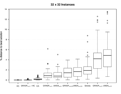
(a)

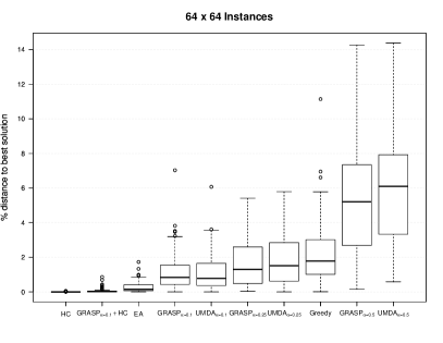
(b)

Figure 5: Relative distances to best solutions of results provided by different algorithms on (a) $32\times 32$ instances and (b) $64\times 64$ instances.

In order to measure performance in a comparable way across the huge collection of problem instances considered, we have recorded the best results found by any algorithm on each instance, and used these to calculate relative deviations to such best known solutions. The results are summarized in Figure 5 showing box plots of the distribution of relative deviations to best known solutions for different algorithms, separately for the $32\times 32$ and $64\times 64$ instances. It can be seen that deviations are very close to 0 for HC, which means that this algorithm was able to provide best known solutions for most of the instances. The EA comes third, with distances that are also quite close to 0. GRASP_α=0.1 and GRASP_α=0.25 are the next two better algorithms, but their performance degrades clearly when compared to HC and EA. The value of upper whisker for the distribution corresponding to Greedy on $32\times 32$ instances is of a 4.59% relative distance to the optimum, whereas the same value for HC is 0% and for EA is 0.48%. The difference is of a 5.78% in the case of $64\times 64$ instances. This is an indications of the extent of improvements achieved by both heuristics over Greedy.

Subsequently, a statistical test was used in order to analyze whether differences among the different techniques are statistically significant. More precisely, the Friedman Test (FT) (Friedman, 1937, 1940), a non-parametric test based on rankings, has been used for this purpose. If, as a result of this test, the null hypothesis stating equality of rankings between the different techniques is rejected, we proceed to post-hoc procedures in order to detect statistical differences among different pairs of algorithms. For this purpose, Shaffer’s static procedure (Shaffer, 1986) with a standard significance level of $\alpha=0.05$ has been used. All these analysis were carried out using the software package provided by the Soft Computing and Intelligent Information Systems group at University of Granada (García and Herrera, 2008).

Table 1: Mean ranks of all algorithms on $32\times 32$ and $64\times 64$ cells instances.

position	algorithm	ranking
1st	HC	1.28
2nd	GRASPα=0.1+HC	1.83
3rd	EA	3.17
4th	GRASPα=0.1	4.82
5th	UMDAα=0.1	4.93
6th	GRASPα=0.25	6.08
7th	UMDAα=0.25	6.75
8th	Greedy	7.39
9th	GRASPα=0.5	8.95
10th	UMDAα=0.5	9.80

Firstly, the mean rank of all ten algorithms in the benchmark considered is computed and shown in Table 1. As can be seen, the order of performance from best to worst is: HC, followed by EA, the two variants of GRASP$|$UMDA using smallest values of $\alpha$, the Greedy algorithm and finally GRASP$|$UMDA_α=0.5. To determine the significance of these rank differences, the FT is performed and results in $\chi^{2}_{F}=1726.18$, much larger than the critical value 16.92 for $\alpha=0.05$ (according to $\chi^{2}$ with 9 degrees of freedom). The $p$-value calculated by this test is actually $p=0$ which provides strong evidence for rejecting equality of rankings. Shaffer’s post-hoc procedure, at the same standard $\alpha=0.05$ level, found statistically significant differences between all pairs of algorithms, except for GRASP_α=0.1 vs UMDA_α=0.1, GRASP_α=0.25 vs UMDA_α=0.25, GRASP_α=0.5 vs UMDA_α=0.5, UMDA_α=0.25 vs Greedy, and HC vs GRASP_α=0.1+HC. It can thus be concluded that using the GRASP_α=0.1 component for initializing solutions for the HC algorithm is not advantageous with respect to using random initialization for this same purpose. Moreover, using the UMDA in order to guide the search of GRASP does not provide benefits with respect to taking random decisions, as it is done in the pure GRASP algorithm. From a more general point of view, all the algorithms proposed in this paper have a better performance than the Greedy algorithm from (Nie et al, 2007), except GRASP_α=0.5 and UMDA_α=0.5 (statistically worse) and UMDA_α=0.25 (better than Greedy but not significantly so). It can be also seen that the performance of GRASP algorithm improves with smaller values of $\alpha$, but this algorithm performs worse than HC and EA for this problem.

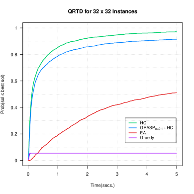
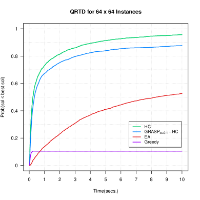
Figure 6: Qualified runtime distributions (QRTD) for best performing algorithms (Greedy also included for comparison purposes) on $32\times 32$ (left) and $64\times 64$ (right) instances. Curves show the probability of reaching best known solutions along time for different algorithms.

The behavior as anytime algorithms of both the best performing heuristics and Greedy is analyzed in Figure 6. This figure shows Qualified Runtime Distributions (QRTD) for the best three algorithms, namely HC, GRASP_α=0.1+HC and EA on $32\times 32$ and $64\times 64$ instances. Such QRTDs show the probabilities of reaching best known solutions as a function of execution time. It can be seen that the algorithm that progresses faster towards high quality solutions is HC. This algorithm is able to find best solutions for 90% of the $32\times 32$ instances in about 1.5 seconds. For $64\times 64$ instances, the same rate of success is achieved after 4.0 seconds of execution. Taking into account the context in which the OPSBD problem should be solved, these seem to be sensible time requirements, amenable for fast-response adjustment of detector locations. From a more detailed point of view, the previous analysis showed that HC and GRASP_α=0.1+HC were roughly equivalent with respect to the quality of solutions they provide, but QRTDs show that GRASP_α=0.1+HC is however slightly slower than HC. As GRASP_α=0.1+HC is a more complicated algorithm to implement and also does not provide advantages over HC, we can conclude that using the latter one is a better alternative to solve this problem. Regarding the EA, QRTDs also show that it progresses at a slower rate than HC, as its curve is always below the one for HC. Finally, although Greedy is not able to progress towards best solutions (it is a deteministic constructive algorithm) its inclusion in the QRTDs allows comparing its performance to the remaining algorithms on a time-quality basis. Notice that compared to the EA, it provides a better solution initially, but the EA can outperform Greedy in a matter of tenths of a second. This is exactly the expected behavior for such a kind of algorithm, as Greedy local decisions can be made in a very fast way but they are expected to be suboptimal in general.

Figure 7: Relative distances to best known solutions of results provided by HC and Greedy on $128\times 128$ instances.

Finally, we compared the best performing algorithm (HC) with the previous proposal in the literature (Greedy) on larger random instances. In this case, maps consisted of $128\times 128$ grids of cells and, for the rest of parameters, we considered the same combinations as those we used previously for $32\times 32$ and $64\times 64$ instances. Maximum allowed execution times were 10 seconds per instance in this case. A Wilconxon signed ranked statistical test rejects the null hypothesis stating equality of rankings between the two algorithms ($p$-value=0). Boxplots for relative distances to best known results are shown in Figure 7. It can be seen that HC algorithm also provides consistently best results for these instances, and that Greedy is not able to provide solutions with same quality. The value of upper whisker for the distribution corresponding to these instances of Greedy is at a 5% relative distance to the optimum, whereas the same value for HC algorithm is 0%.

4.2 Sensitivity Analysis

In this section, we perform a sensitivity analysis on the performance of the Hill Climbing algorithm (Section 3.4) with respect to Greedy (Section 3.2) with the aim of studying which parameter settings of the problem lead to a larger performance gap among these two techniques. The rationale for this procedure is that if the relative improvement of the solution provided by Hill Climbing over Greedy increases for some parameter settings, it can be considered that those instances turn out to be harder-to-solve for the latter. The different parameters and settings that have been analyzed are a superset of those considered in the previous section, namely:

• Maps with dimensions of $32\times 32$ and $64\times 64$ cells.

• Different side lengths for cells comprising the maps: $\zeta\in\{5,10,20\}$ meters.

• Different number on entrances on each border of the map in $\{2,3,4\}$ leading to $\varepsilon\in\{8,12,16\}$.

• Different number of objective cells on the map: $\phi\in\{2,4,6,8\}$.

• Different percentages of blocked cells on the map: $\varpi\in\{2.5\%,5\%,10\%\}$.

• Different number of detectors to be placed on the map: $\delta\in\{2,4,6,8,10\}$.

• Different values of the detection radius: $\tau\in\{10,20,40\}$ meters.

All possible combinations of these parameter settings lead to 3,240 different kinds of instances, and for each of them, we have considered 25 random instances, so that our analysis comprises a total of 81,000 different instances. In the case of $32\times 32$ cell maps, the maximum execution time allowed for the algorithms on each instances was 5 seconds whereas in the case of $64\times 64$ maps, this time was extended to 10 seconds.

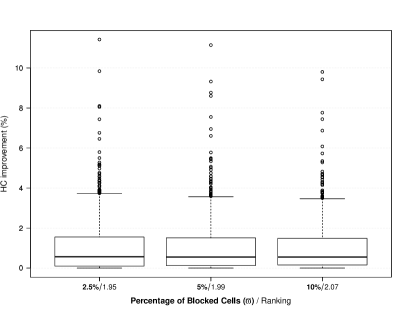
Figure 8: Relative improvements of HC over Greedy for different percentages of blocked cells ($\varpi$) in the map. Settings are ordered (left to right) from more difficult to easier ones. Rankings are shown at the right side of labels. In order to interpret this figure and subsequent ones in this subsection, notice that the boxplots depict the distribution of the aggregated data and show the range of variation in each case, whereas the rankings are computed by aligning the results obtained by each algorithm on the instances generated by each parameter combination and are used by the statistical tests.

4.2.1 Percentage of Blocked Cells

We firstly analyzed differences between maps with varying percentages of blocked cells ($\varpi\in\{2.5\%,5\%,10\%\}$). The ranking is shown in Figure 8. The value of the Friedman statistic is $\chi^{2}_{F}=7.59$ that corresponds to a $p$-value = $0.02$ (the critical value is in this case is distributed according to $\chi^{2}$ with 2 degrees of freedom, yielding $5.99$). This provides evidence for rejecting the null hypothesis that states equality of rankings between the different settings for $\varpi$. The order in Figure 8 goes from more difficult instances to easier ones, so that the first position corresponds to the setting for which the Hill Climbing algorithm provides the largest improvement. Post-hoc procedures only show statistical significant differences, at the standard significance level of $\alpha=0.05$, between configurations for $\varpi$ parameter of 2.5% vs 10%. Thus, it can be seen that a lower percentage of blocked cells leads to maps that are harder to solve for Greedy, but also that there are no differences between the intermediate setting for this parameter and the smaller or larger ones. We interpret this result in terms of the broader dispersion of shortest paths in instances with fewer obstacles, which makes more difficult to find major cross points and hence the goodness of solutions relies on the distribution of detectors with a more global perspective, as opposed to covering a couple of critical points and use the remaining detectors for fine tuning.

4.2.2 Side Length of Cells

Regarding side lengths of cells ($\zeta$) in the grid, the ranking is shown in Figure 9. We obtain $\chi^{2}_{F}=518.25$, corresponding to a $p$-value = $2.34\cdot 10^{-10}$ (the critical value is here distributed again according to $\chi^{2}$ with 2 degrees of freedom, yielding $5.99$). Thus, there is strong evidence for rejecting the null hypothesis that states equality of rankings between the different settings for $\zeta$. In this case, post-hoc procedures found statistically significant differences (at the standard significance level of $\alpha=0.05$) between all possible settings for this parameter. It can be seen that the difficulty of instances increases as cell sizes decrease. One possible explanation for this phenomenon may be that having a more fine-grained map allows for a more precise placement of detectors in the map. This seems to be better exploited by Hill Climbing, that has more choices for fine-tuning the solution from a global perspective (as opposed to the local approach of Greedy).

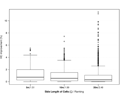
Figure 9: Relative improvements of HC over Greedy for different side lengths ($\zeta$) of cells in the grid. Settings are ordered (left to right) from more difficult to easier ones. Rankings are shown at the right side of labels.

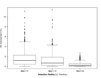
Figure 10: Relative improvements of HC over Greedy for different values of the detection radius ($\tau$). Settings are ordered (left to right) from more difficult to easier ones. Rankings are shown at the right side of labels.

4.2.3 Detection Radius

The detectors placed in the map may have a different radius of effectiveness. Here we consider settings for this parameter in $\tau\in\{10{\rm m},20{\rm m},40{\rm m}\}$. The resulting ranking is shown in Figure 10. We obtain $\chi^{2}_{F}=825.17$, corresponding to a $p$-value = $2.9\cdot 10^{-10}$ (the critical value is once again distributed according to $\chi^{2}$ with 2 degrees of freedom). Hence, the null hypothesis stating equality of rankings between the different settings for this parameter should be rejected. In the case of this parameter, post-hoc procedures found statistically significant differences (at the standard significance level of $\alpha=0.05$) between all pairs of settings. It must be noted that for this parameter harder instances are those with an intermediate radius of detection. One interpretation of these results may be that a smaller radius leads to less interactions between the detectors and paths followed by terrorists, whereas a very large radius allows for one detector to cover a great extent of the map, thus simplifying the difficulty of the problem. It is the intermediate radius $\tau=20$m that leads to harder instances in this case as there is a good degree of interaction of each detector with different paths and, at the same time, the radius is small enough for a precise placement of the detector to turn out to be crucial. Of course, this effect also depends on the number of detectors to be placed since, if this number is large, a suboptimal placement of some detectors may be to some extent compensated by other detectors covering the same paths. In this case, the smaller the detection radius, the more influential the location of the detectors would become.

4.2.4 Number of Detectors

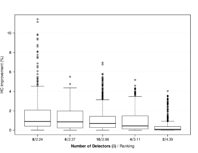
Figure 11: Relative improvements of HC over Greedy for different number of detectors ($\delta$) placed on the map. Settings are ordered (left to right) from more difficult to easier ones. Rankings are shown at the right side of labels.

We have considered different number of detectors ($\delta$) to be placed on the map. Rankings are shown in Figure 11. The associated Friedman statistic is $\chi^{2}_{F}=763.50$ which implies a $p$-value = $2.41\cdot 10^{-10}$ (the critical value is in this case distributed according to $\chi^{2}$ with 4 degrees of freedom, yielding $9.49$) and thus there are significant differences for different settings of this parameter. Post-hoc procedures found statistically significant differences (at the standard significance level of $\alpha=0.05$) between all pairs of settings except for 6 vs. 8. Results show that instances with a smaller number of detectors ($\delta\in\{2,4\}$) are the easiest ones, but also that instances with the maximum number of detectors ($\delta$=10) are easier than those with 8 and 6 detectors. One interpretation of these results is that the search space for a small number of detectors is relatively easy to explore for different algorithms, but also that having a higher number of detectors allows for placing them in a less precise way without affecting in a significant way the quality of the solution. In other words, instances with an intermediate number of detectors lead to a large enough search space which raises the difficulty of the problem. At the same time, a precise placement of the limited number of available detectors is required in order to provide high-quality solutions for these instances.

4.2.5 Number of Entrances

Figure 12: Relative improvements of HC over Greedy for different number of entrances ($\varepsilon$) on the map. Settings are ordered (left to right) from more difficult to easier ones. Rankings are shown at the right side of labels.

Regarding the number of entrances on the map ($\varepsilon$), we have considered 2, 3 and 4 entrances on each side of the map, which leads to the following settings: $\varepsilon\in\{8,12,16\}$. Rankings are shown in Figure 12. The Friedman statistic is $\chi^{2}_{F}=202.47$ and the corresponding $p$-value is $9.97\cdot 10^{-11}$ (the critical value is in this case distributed according to $\chi^{2}$ with 2 degrees of freedom, yielding $5.99$). Post-hoc procedures found differences (at the standard significance level of $\alpha=0.05$) between all pairs of settings for this parameter. In this case, the larger the number of entrances, the easier the resulting problem instances are. This result can be interpreted in terms of the number of paths (which is proportional to the number of entrances). Recall that the probability of targeting a certain objective is distributed across the different paths emanating from each entrance. Therefore, the larger the number of entrances, the smaller the weight of individual paths. This means that adjusting the precise location of a detector will yield a smaller variation of the objective function as a result of the the different coverage of the numerous existing paths. Of course, we cannot take this argument to the opposite limit because if the number of entrances was very low it would be easy to cover the paths by any appropriate heuristic.

4.2.6 Number of Objectives

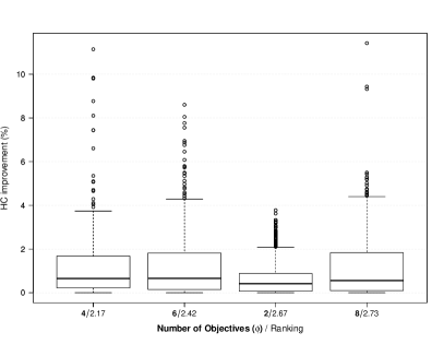
Figure 13: Relative improvements of HC over Greedy for different number of objectives ($\phi$) on the map. Settings are ordered (left to right) from more difficult to easier ones. Rankings are shown at the right side of labels.

Here we consider maps with different numbers of objective cells ($\phi\in\{2,4,6,8\}$). Rankings are shown in Figure 13. The Friedman statistic is $\chi^{2}_{F}=94.69$, implying a $p$-value = $5,74\cdot 10^{-11}$ (the critical value is in this case distributed according to $\chi^{2}$ with 3 degrees of freedom, yielding $7.81$). Post-hoc procedures in this case show that there are not statistically significant differences (at the standard significance level of $\alpha=0.05$) between maps with 2 and 8 objectives. In this case, instances with the lowest ($\phi=2$) and highest ($\phi=8$) number of objectives are thus indistinguishable, and both lead to easiest-to-solve instances. For intermediate settings of this parameter, instances with $\phi=4$ are harder-to-solve than those with $\phi=6$. These results are partly explained in accordance to the argument laid down in Section 4.2.5 for the number of entrances, since the number of paths is also proportional to the number of objectives. In this sense, the lower limit ($\phi=2$) correspond to instances in which there can be little variation of quality in solutions because most paths leading to objectives can be adequately covered. Similarly, in the upper limit ($\phi=8$) the detectors need to cover much ground and as a result adjusting the location of a detector placed by Greedy can increase the coverage of some paths at the expense of others, resulting in the smallest window of improvements.

4.3 Real Instances

Finally, we have deployed Hill Climbing and Greedy on some more realistic instances resembling the features exhibited by urban areas that might be subject to a terrorist attack. These are depicted in Figures LABEL:fig:mapsReal:map1–LABEL:fig:mapsReal:map3 and comprise three different scenarios: (1) a large square, (2) an old-town area and (3) a mixture of the previous two – see Table 2. All of them have been constructed based on real-world locations. Objectives in these scenarios correspond to typical crowded places such as cafe terraces, small flea-markets or bazaars, or monuments with great touristic attractive and other iconic landmarks that gather people around them. All scenarios are represented on a $32\times 32$ grid. These instances will be used to test the comparative performance of both algorithms (Hill Climbing and Greedy) in a more pragmatic context, identifying the circumstances under which there is a larger quality gap between them and how different the solutions provided by either algorithm are from a structural point of view.

Table 2: Description of the three realistic scenarios considered in the experimentation.

		Number of	Number of
Name	Area (m2)	entrances ($\varepsilon$)	objectives ($\phi$)	Description
map1	$160\times 160$	22	61	A large square surrounded by buildings and with only a few entrances, in which several monuments and other obstacles are scattered.
map2	$224\times 224$	16	25	An old-town area featuring small plazas and curvy, non-perpendicular streets that connect them.
map3	$352\times 352$	11	9	A mixture of the two previous scenarios that includes a large square and some adjacent streets

(a)

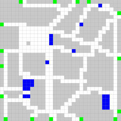
(b)

(c)

Figure 14: Realistic maps considered. (a) A large plaza in the city center. (b) An old-town urban area with curvy streets and small plazas. (c) A mixed scenario including both a large plaza and some adjacent streets.

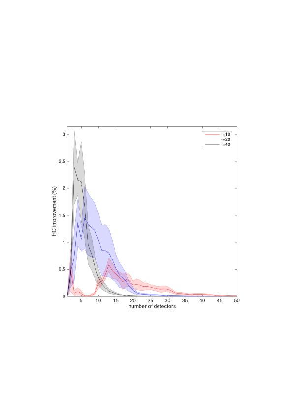
(a)

(b)

Figure 15: (a) Relative improvement of solutions provided by HC over those provided by Greedy algorithm across the three scenarios, as a function of the number of detectors $\delta$ for different values of the detection radius $\tau$. The shaded areas indicate the standard error. (b) Cumulative distribution of improvements depending on the detection radius $\tau$. The inner quartiles are shown.

The experimentation has been done with a number of detectors $\delta$ ranging from 1 to 50 and for different values of the detector radius $\tau\in\{10,20,40\}$ meters. All experiments have been replicated 25 times for each combination of map, number of detectors and detection radius. We let the Hill Climbing algorithm run for 10 seconds or until an local optimum was found (cf. Algorithm 3). This resulted in Hill Climbing taking an average of 4.45 seconds to provide its final solution (standard error $\sigma_{\bar{x}}=0.043$s). Hill Climbing has consistently found the same solution in each case (Greedy is deterministic and therefore only one run is required per test case). The results are summarized in Figure LABEL:fig:real:HCvsGreedyRadius, in which the average relative improvement of Hill Climbing over Greedy is shown. As can be seen, this improvement is always positive for any number of detectors. Indeed, this improvement is statistically significant ($p$-value $\approx 0$) according to a Wilcoxon signed rank test for any scenario and detection radius, except for map₃ and $\tau=40$. Aggregating the results for all values of $\tau$, the improvement is also statistically significant for all scenarios (again $p$-value $\approx 0$). Not surprisingly, the relative improvement initially increases when more detectors are used, and then declines after reaching a certain peak. Obviously, as more and more detectors are placed the fitness function starts to saturate (recall Equation 7 – when the coverage of the paths is large, an additional increase in this coverage only implies a small fitness increase due to the exponential decay of the last term of the equation). It is nevertheless interesting to note two qualitative differences in behavior depending on the value of the detection radius. Firstly, as $\tau$ decreases, the peak is located in an interval comprising more detectors. This is more precisely depicted in Figure LABEL:fig:real:HCvsGreedyCDF, in which the cumulative distribution of improvement is shown (normalized in terms of percentiles for comparison purposes). If we focus on the central half of the distribution (that is, the second and third quartiles), it comprises $\delta\in[4,7]$ for $\tau=40$m, $\delta\in[6,12]$ for $\tau=20$m, and $\delta\in[13,24]$ for $\tau=10$m. This can be interpreted in terms of the area covered by each detector in that case: as the detection radius increases, larger segments of the paths can be covered and therefore the fitness functions starts to saturate at an earlier point than it would for smaller detection radius. In the latter case, adjusting the location of detectors result in comparatively smaller length variations in the paths covered, implying that the fitness function saturates more slowly (and hence for a larger interval of detectors) and relative improvements are comparatively smaller than for larger values of the detection radius. Indeed, if we perform a head-to-head comparison among the values obtained on each map and number of detectors for each value of $\tau$, we observe that $\tau=10$ ranks better than $\tau\in\{20,40\}$ (mean ranks are 1.48, 1.87 and 2.65 respectively), the differences being statistically significant (Friedman test $p$-value $\approx 0$, Shaffer’s test passed at $\alpha=0.05$ for all pairs of values of $\tau$). This is in agreement with the interpretation laid down in Section 4.2 for random instances, and underlines the larger interval for which improvements are obtained for decreasing values of the detector radius.

(a)

(b)

Figure 16: Solutions found for map₂ using $\delta=6$ detectors of radius $\tau=40$m. (a) Greedy (b) Hill Climbing. The numbers close to detector locations in the left image indicate the order in which Greedy places the detectors.

Figure 16 show a comparison of the solutions found by Greedy and Hill Climbing on a specific case, namely the old-town scenario with $\delta=6$ and $\tau=40$m. Notice how the solution created by Greedy places the first three detectors trying to cover the densest target areas. Then, it tends to place the next two detectors in partial overlap with the first two, aiming to maximize the coverage of these areas by virtue of the independent functioning of the detectors. Finally, the last detector is placed close to a corner of the map, covering paths originating in two entrances. On the other hand, the solution provided by Hill Climbing has three detectors in locations rather close, but not identical, to the first three detectors placed by Greedy. This slight variation in their locations allows to place the remaining three in strategical positions to cover all paths originating in the four upper entrances, in three of the lower entrances, and in one of the entrances in the right part whose paths were receiving less attention by Greedy. Overall, the solution found by Hill Climbing has a more global rationale and looks more spatially balanced.

5 Conclusions

Suicide bombing is an infamous form of terrorism that presently causes a large number of casualties worldwide. In this work we have researched the problem of placing a number of non-fully reliable detectors on a threat area with known targets with the aim of maximizing chances of detecting a suicide-bombing attack, thus minimizing the expected number of casualties.

Apart from a branch-and-bound algorithm that does not scale well with problem size, the only previous proposal in the literature to tackle this problem was a greedy algorithm. We have approached this problem for the first time to the best of our knowledge from the point of view of iterative heuristics and metaheuristic techniques. To this end, we firstly performed an experimental comparison of the different proposed algorithms on a benchmark comprising a large set of random instances with different parameterizations. Results indicate that, among all considered techniques, a Hill Climbing algorithm obtains the best results in a consistent way, clearly outperforming the previous proposal from the literature. Secondly, we did a sensitivity analysis in order to determine those settings of problem parameters leading to harder-to-solve instances. Thirdly, the Hill Climbing heuristic (as the best performing algorithm) was experimentally compared to the greedy algorithm (as the previous approach in the literature) on a set of real world scenarios that could be subject to terrorist attacks. Results of these tests corroborate the good performance of Hill Climbing observed before.

Different lines of research are open as future work to the present study. First of all, alternative algorithmic approaches can be explored. For instance, we have observed that the proposed UMDA is able to outperform GRASP in case the maximum allowed execution time is increased. Designing an alternative probabilistic model or performing new experimental comparisons with increased allowed execution times constitute promising extensions to this paper. Another promising proposal is to hybridize in a synergistic way the EA and Hill Climbing algorithms, as best performing algorithms studied in this work. To this end, Memetic Algorithms (Neri et al, 2012) constitute a well established and successful framework that can be used for this purpose. Lastly, more sophisticated versions of the problem studied could be also tackled in future work, like, for instance, considering more precise models of the functioning of detectors or making dynamic the locations of targets, so that their situation and even their number may vary along time.