Symbolic Regression for Beyond the Standard Model Physics

Abstract

We propose symbolic regression as a powerful tool for studying Beyond the Standard Model physics. As a benchmark model, we consider the so-called Constrained Minimal Supersymmetric Standard Model, which has a four-dimensional parameter space defined at the GUT scale. We provide a set of analytical expressions that reproduce three low-energy observables of interest in terms of the parameters of the theory: the Higgs mass, the contribution to the anomalous magnetic moment of the muon, and the cold dark matter relic density. To demonstrate the power of the approach, we employ the symbolic expressions in a global fits analysis to derive the posterior probability densities of the parameters, which are obtained extremely rapidly in comparison with conventional methods.

The chief test of any proposal for Beyond the Standard Model (BSM) physics is to confront it with experimental data. The standard approach is well trodden: first one chooses a reasonable parameter space motivated by a combination of physical argumentation and expediency; for each point in the parameter space the physical low-energy spectrum is determined and possibly an initial cut made for phenomenological viability (for example in supersymmetry (SUSY) the mass and charge of the lightest SUSY partner); for each remaining viable point the cross-sections are calculated and the relevant observables determined such as dark matter relic density, anomalous magnetic moment of the muon, and so forth; finally with this information to hand each point can be evaluated and assessed. One can then attempt to scan the entire parameter space this way, or alternatively use a Markov Chain Monte Carlo or nested sampling algorithm [1, 2, 3], such as that in MultiNest [4], to arrive at posterior probability densities for the parameters.

This approach has the appeal of being directly connected to the underlying physics, but it suffers from a severe bottleneck, namely the computation of the observables. Indeed each one of them is the result of a painstaking physical analysis which may need to encompass many subtle effects (for example, three loop running from the Grand Unified Theory (GUT) scale, co-annihilation for dark matter relic density and so forth). Typically, this leads to a chain of computation to get from the input parameters to the low-energy observables. Thus, although closed-form expressions for the observables in terms of the input parameters are in principle “knowable” (at least in perturbation theory), they would be exceedingly complex and could not be usefully expressed analytically except possibly in the case of a restricted set of observables in extreme limits of parameter space.

To avoid this bottleneck, it is natural to turn to machine learning to bypass the computation chain or more efficiently sample points of interest (for recent examples and applications, see Refs. [5, 6, 7, 8, 9]). However, the negative aspect of machine learning is that it is generally neither interpretable nor explainable.

This lack of interpretability (by which we mean an inability to be able to understand the dependence of the observables on the input parameters) is frustrating because certain correlations between input parameters and observables can be motivated by physical arguments. For example, it is clear that SUSY contributions to $(g-2)_{\mu}$, the anomalous magnetic moment of the muon, generally decrease with increasing values of the soft SUSY-breaking parameters because the superpartner states begin to decouple. This correlation provides a modest degree of explainability, but one feels that there must exist analytic expressions that can more finely reproduce the dependence of the low-energy observables on the parameters. Indeed if it were possible to infinitely refine such expressions, then the end result would be a set of analytic formulae that would accurately predict all low-energy observables from any given set of input parameters, with no need for time-consuming computation.

The business of producing simple analytic expressions that reproduce the output of complicated computations is known as symbolic regression [10]. In the physics context, it has most famously been discussed in generality in Ref. [11] and for specific applications in Refs. [12, 13, 14, 15, 16, 17]. Symbolic regression attempts to provide analytic expressions for the outputs by learning the symbolic formulae that best fit the observed results. It does not attempt to provide any kind of rationale for the expressions it finds (although as in Ref. [11] the bank of symbolic expressions which are considered can be motivated by physics), the goal being merely to discover the simplest and most accurate analytic expressions that reproduce the observables in the region of the parameter-space of interest. This is a useful compromise: if we are prepared to forego the physically organised chain of computation that determines the observables at each point in parameter space, then we can gain much greater analytic power.

The purpose of this letter is to demonstrate that symbolic regression is a powerful tool for studying BSM physics. As a benchmark model, we will consider the so-called Constrained Minimal Supersymmetric Standard Model (CMSSM), which has a four-dimensional parameter space, consisting of GUT scale degenerate gaugino masses, scalar masses, and universal trilinear coupling, and the electroweak scale Higgs Vacuum Expectation Value (VEV) ratio, denoted respectively as $m_{1/2},\leavevmode\nobreak\ m_{0},\leavevmode\nobreak\ A_{0}$ and $\tan\beta$. We provide a set of analytical expressions that reproduce the Higgs mass, $m_{H^{0}}$, the SUSY contribution to the muon anomalous magnetic moment, $\delta(g-2)_{\mu}$, and the dark matter relic density, $\Omega_{\rm DM}h^{2}$, in terms of these parameters (which are available at [18] alongside the code that produced them, and the dataset used can be found at [19]). In addition we provide a “classifier” $C(m_{1/2},m_{0},A_{0},\tan\beta)$, which is a function that takes values greater than $0.5$ when a point is physically viable in the sense that it has neutral dark matter, lack of charge and colour breaking minima, and a positive dark matter relic density. As an example application of our methodology, we will demonstrate that by employing these symbolic expressions one may determine the posterior probabilities of the CMSSM extremely rapidly compared to conventional methods.

There are several approaches to symbolic regression that could be considered for this purpose, ranging from evolutionary methods to transformer-based neural networks. A comprehensive overview and comparison of symbolic regression methods is included in Refs. [20, 21, 22, 23, 24]. However, the specific properties that we require of a symbolic regressor for this letter, and for BSM more generally, are somewhat specific to BSM physics. Not only is the parameter space often high dimensional, but also it tends to contain fairly focussed regions of interest which are localised around poles and mass-degeneracies, and these need to be captured by the expressions. Consequently, successful training involves a large and relatively fine multidimensional set of training data. This excludes the most commonly used symbolic regression packages (e.g. PySR) and favours Operon (and its Pythonically wrapped version, PyOperon) [25], due to its highly efficient vectorised structure and low memory footprint.

Analytic expressions for the MSSM.—

Operon is a framework for symbolic regression based on Genetic Programming (GP), which is an evolutionary method in which each individual in the population is an expression tree that represents a symbolic expression built from a bank of pre-chosen functions. Evolution of the population is then simulated by repeated cycles of selection, breeding, and mutation. The selection probability for breeding is governed by a loss-function for each individual, which is determined from the properties of the symbolic formula that is generated by its expression tree.

Obviously, these properties include closeness to the training data (which in this study is a set of $10^{5}$ predetermined CMSSM points), but also the properties of the expression itself. The SymbolicRegressor module of PyOperon runs the GP loop with two objectives: one of several possible regression metrics and the “length” of the expression itself. The regression metric is a user-defined hyperparameter that can be chosen from one of the following: “mean square error”, “mean average error”, “$r^{2}$”, and “normalised mean square error”. The “length” is simply the number of characters (string length) of the mathematical expression. During the GP loop, the population is evaluated on these two metrics, with the best individuals being those inhabiting the corresponding Pareto front. At the end of the run (i.e. after the specified number of generations/budget is exhausted), SymbolicRegressor returns all the Pareto front individuals.

To optimise the regression metrics, an Optuna loop was implemented in our analysis. This uses a Tree Parzen Estimator (TPE), a Bayesian optimisation algorithm, to determine the best hyperparameters in the algorithm, which, as well as the regression metrics, include for example population size, population initialisation, and so forth (see Ref. [25]). As a “figure of merit” for a particular choice of hyperparameters, we use the relative error of each of the three observables for each individual in the final Pareto front. Denoting the observables generically as $y$, this is given by $|y_{\rm pred}-y_{\rm true}|/|y_{\rm true}|,$ where $y_{\rm true}$ are points taken from the validation set (also composed of $10^{5}$ points).

The relative error was preferred over other more common regression metrics, such as $r^{2}$, because the latter tend to be biased toward higher nominal values, which can be problematic for observables that span multiple orders of magnitude. The average of the relative errors was taken, weighted by “flattening weights” which level the distribution to ensure that the regressor performs well over the whole range of values of the observable, thus preventing it from focusing on the most common values of the observable. Therefore, during training, because Operon does not use sample weights to produce weighted averages when computing the loss function, at each Optuna iteration, the training data were resampled without replacement according to the “flattening weights”, which ultimately reduced our useable dataset from $10^{5}$ to $10^{4}$ data points, while ensuring a mostly flat distribution of the target observable.

Such weighting is an important feature especially for $\Omega_{\rm DM}h^{2}$ because its values range over many orders of magnitude, and, as we shall see, it poses by far the most challenging regression problem in this study. In fact, without resampling the training data to produce a flat distribution the symbolic regressor was unable to accurately map the physical region of interest $\mathcal{O}(\Omega_{\rm DM}h^{2})\sim 0.1$, due to the relative scarcity of points with values in that range. By producing a flatter $\mathcal{O}(\Omega_{\rm DM}h^{2})$ distribution during training, this was greatly improved, but there was still considerable contamination in the range of physical interest. Further significant improvement was achieved by allowing a larger budget and a larger maximal tree-size for both $\Omega_{\rm DM}h^{2}$ and $m_{H^{0}}$, and rerunning the Optuna loop to produce their final expressions. Meanwhile, for $\delta(g-2)_{\mu}$ and the classifier it was sufficient to keep the smaller expressions obtained with a smaller budget.

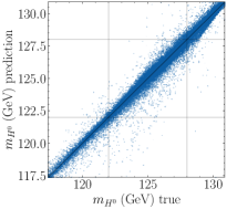
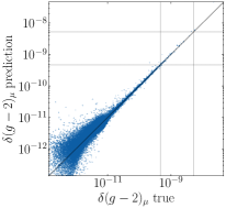
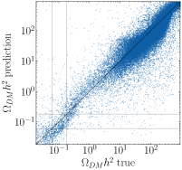
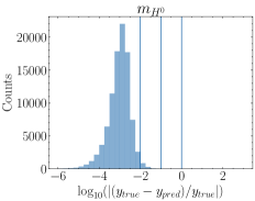
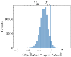
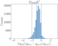
Figure 1: Symbolic regressors’ performance on the test set. Upper panels: “true vs. prediction” scatter plots, the solid lines marking the boundary of the physically viable values of the observables. Lower panels: distribution of relative errors, the vertical lines offering a visual guide for relative errors of order 1%, 10%, and 100%.

To evaluate the quality of the symbolic regressors that were obtained with this procedure, we present in Fig. 1 the “true vs. prediction” scatter plots (upper panels) and the distribution of the relative errors of the predictions (lower panels), produced using the test set. It can be seen that for the Higgs mass the regression is very accurate throughout all the values, with virtually every point having a relative error below 1%. For $\delta(g-2)_{\mu}$ the relative errors are greater, but importantly remain diminishingly small in the region of physical viability (where $\delta(g-2)_{\mu}$ is enhanced). (The distribution of points is typical of a regressor with a constant absolute error.) For $\Omega_{\rm DM}h^{2}$ relative errors are on average above 10%. This is actually better than the 20% theoretical error that is typically assigned to $\Omega_{\rm DM}h^{2}$ in global fit analyses. Despite this, the symbolic regressor is capable of producing viable estimates in the physical region of interest. It is important to note that each scatter plot shows $10^{5}$ points of the test set, and the points with poor predictions in the upper panels of Fig. 1 are actually very few, constituting only a small scattered minority of the test set (as is evident in the lower panels of Fig. 1).

Application: global fits.—

Generally, to make convergent and statistically robust global fits, say using state-of-the-art nested sampling algorithms, the main difficulty is the need to draw samples at each iteration of the algorithm, until a point is found that has a likelihood greater than that of the lowest point within the likelihood-sorted live points. There are various approaches to achieving this with varying costs to compute the usually simulation-based or scientific software package-based likelihoods. Hence, we would now like to demonstrate that a complete or partial replacement with symbolic expressions of the high energy physics packages employed for making BSM global analyses is a solution to the resource problems that are associated with the stringent experimental limits and the non-observation of new fundamental particles.

For our benchmark model, the CMSSM, the observables $m_{H^{0}}$, $\Omega_{\rm DM}h^{2}$, and $\delta(g-2)_{\mu}$ can be computed for each point in the parameter space via particle spectrum generators such as SPheno [26] and particle dark matter packages such as MicrOMEGAs [27]. We use the most precise Higgs boson measurement, $m_{H^{0}}=125.04\pm 0.12$ GeV [28] and $\Omega_{\rm DM}h^{2}=0.12\pm 0.0012$ [29] but include the aforementioned theoretical uncertainty of 20% in predicting the relic density. Thus, $\Omega_{\rm DM}h^{2}=0.12\pm 0.02$ is used for the fits. The discrepancy between the high precision Standard Model (SM) prediction for the muon anomalous magnetic moment [30] and the experimental measurements [31] which we adopt for the fits is $\delta(g-2)_{\mu}=(249\pm 48)\times 10^{-11}$. These constitute the set of data, $\underline{d}=\{\mu_{i}\pm\sigma_{i}\}$ that we use to make the global fit, where $\mu_{i}$ and $\sigma_{i}$ represent the measurement central values and uncertainties for the above observables (with $i=1,2,3$).

The CMSSM parameters were sampled from uniformly distributed prior probability densities, which were respectively within $[0,10]$ TeV for $m_{1/2}$ and $m_{0}$, $[-6,6]$ TeV for $A_{0}$, and $[1.5,50]$ for $\tan\beta$. For each point in the parameter space, $\underline{\theta}=\{m_{1/2},m_{0},A_{0},\tan\beta\}$, the likelihood is estimated as

$$p(\underline{d}|\underline{\theta})\leavevmode\nobreak\ =\leavevmode\nobreak\ \prod_{j=1}^{3}\,\frac{1}{\sigma_{j}\sqrt{2\pi}}\,exp\bigg{\{}\frac{-(y_{\rm pred}^{j}-\mu_{j})^{2}}{2\sigma_{j}^{2}}\bigg{\}}\leavevmode\nobreak\ ,$$ (1)

where again $y_{\rm pred}^{j}$ represents the predictions for our three observables. For running the nested sampling algorithm, we used version 3.10 of MultiNest with 4000 live points in the nested importance sampling mode and with tuning parameters chosen as $\mbox{\tt mmodal}=1$, $\mbox{\tt ceff}=0$, $\mbox{\tt efr}=1.8$, $\mbox{\tt tol}=0.5,$ and $\mbox{\tt seed}=-1.$

For the comparator analysis using symbolic regression, we adopted a “hybrid” approach, which utilises the symbolic expressions in place of the SPheno package predictions for $m_{H_{0}}$ and $\delta(g-2)_{\mu}$, while using the MicrOMEGAs package for the relic density prediction.

We find that the hybrid global fit analysis compares exceedingly well with that made using the conventional method (packages-based). To illustrate, Fig. 2 shows the posterior distributions of the CMSSM parameters fit to our three observables using MultiNest and plotted using GetDist [32]. The 65% and 95% Bayesian probability contour lines (in red on the 2-dimensional plots, and labelled “Expressions” in the legend) represent the 2-dimensional posterior distributions from the hybrid fit, while the 2-dimensional scatter plots (with points coloured according to the Higgs mass, and labelled “Packages” on the legend) represent the conventional fit in which all the observables are computed with packages. These results are clearly in excellent agreement, confirming that the dynamical features of the symbolic expressions correctly approximate those of the SPheno package.

Figure 2: The posterior distributions from a solely packages-based (2-dimensional scatter plots on the off-diagonal entries, and black lines on the 1-dimensional plots) versus hybrid package+expressions based (the red lines) global fits of the CMSSM parameters to $m_{H^{0}}$, $\delta(g-2)_{\mu}$, and $\Omega_{\rm DM}h^{2}$. For the hybrid fits the symbolic expressions for $m_{H^{0}}$ and $\delta(g-2)_{\mu}$ were used while the MicrOMEGAs package was used for computing $\Omega_{\rm DM}h^{2}$. Mass dimensionful parameters are in GeV.

Additional evidence of the agreement between the two fits can be obtained from the central values and dispersions of the CMSSM parameters’ posteriors. In Table 1, we show the logarithm of the Bayesian evidence, $\log_{e}Z$, returned by MultiNest at the end of the fits, and quote the mean and standard deviations for the CMSSM parameters.

	$\log_{e}Z$	$m_{1/2}$	$m_{0}$	$A_{0}$	$\tan\beta$
Packages	$4.48\pm 0.07$	$3.68\pm 0.56$	$8.93\pm 0.48$	$1.23\pm 2.66$	$34.62\pm 10.71$
Expressions	$4.90\pm 0.15$	$3.69\pm 0.59$	$8.99\pm 0.48$	$1.36\pm 2.84$	$30.72\pm 10.36$

Table 1: The CMSSM importance nested sampling log-evidence values and parameter estimates returned by MultiNest based on the packages- versus expressions-based (hybrid here) global fits. Mass dimensionful parameters are in TeV.

Discussion.—

Generally, one anticipates a huge reduction in the computational resources required to perform a global fit using symbolic regression: for example, we find that two orders of magnitude less CPU time would be required for the CMSSM global fit with all three of our observables computed using the symbolic expressions. However it is interesting to note that symbolically regressed expressions can be in conflict, and some care must be taken in using them according to the physical problem. In fact, this partly motivated our choice of these three observables for this particular study. Indeed, studying our training data points in a frequentist fashion reveals that good $\Omega_{\rm DM}h^{2}$ values are mostly obtained for Higgsino dark matter, whereas good $\delta(g-2)_{\mu}$ values are mostly obtained for Bino dark matter. In other words, good values for these two observables are relatively rare in the CMSSM parameter space, and the most populated regions do not overlap. Thus our symbolic expressions for $\Omega h^{2}$ are not sensitive to those very rare points that also have the required $\delta(g-2)_{\mu}$ contribution, but are instead swamped by Higgsino dark matter points. Therefore if one wished to achieve a similarly good global fit using symbolic expressions for all three observables one should proceed by first including into the classifier regressor the requirement that the dark matter candidate should be Bino-like. This and similar refinements will be the subject of future work.

As a final comment, we remark that as well as offering a different and very efficient way of analysing BSM models, symbolic regression opens up several new avenues for analysing high energy physics models. As an example, it is interesting to note that it may now be possible to perform global fit analyses on a quantum computer in a manner analogous to that in Ref. [33], but instead by directly encoding the symbolic expressions for the observables in the quantum circuit. This kind of analysis would be out of the question using the conventional calculational route due to the impossibility of fully encoding the required chain of computation in a quantum circuit. Another promising application of our approach is to further the potential of differentiable and probabilistic programming in BSM studies, where the symbolic expressions can replace the black-box imposed by the computational packages.

We are extremely grateful to Bogdan Burlecu and Gabriel Kronberger for extensive guidance with Operon. We would like to thank Miles Cranmer and Pedro Ferreira for help and discussions. SA₁ and SA₂ thank CERN-TH and SA₁ thanks the Institute for Theoretical Physics at Heidelberg University for hospitality extended during the initial stages of this work. SA₂ and MCR are supported by the STFC under Grant No. ST/T001011/1. This work was performed using resources provided by the Cambridge CSD3, provided by Dell EMC and Intel using Tier-2 funding from EPSRC grant EP/T022159/1, and DiRAC funding from the STFC.

References

- [1] J. Skilling, “Nested Sampling,” AIP Conf. Proc. 735 no. 1, (2004) 395.
- [2] J. Skilling, “Nested sampling for general Bayesian computation,” Bayesian Analysis 1 no. 4, (2006) 833–859.
- [3] G. Ashton et al., “Nested sampling for physical scientists,” Nature 2 (2022) , [arXiv:2205.15570 [stat.CO]].
- [4] F. Feroz and M. P. Hobson, “Multimodal nested sampling: an efficient and robust alternative to MCMC methods for astronomical data analysis,” Mon. Not. Roy. Astron. Soc. 384 (2008) 449, [arXiv:0704.3704 [astro-ph]].
- [5] S. Caron, J. S. Kim, K. Rolbiecki, R. Ruiz de Austri, and B. Stienen, “The BSM-AI project: SUSY-AI–generalizing LHC limits on supersymmetry with machine learning,” Eur. Phys. J. C 77 no. 4, (2017) 257, [arXiv:1605.02797 [hep-ph]].
- [6] A. Hammad, M. Park, R. Ramos, and P. Saha, “Exploration of parameter spaces assisted by machine learning,” Comput. Phys. Commun. 293 (2023) 108902, [arXiv:2207.09959 [hep-ph]].
- [7] F. A. de Souza, M. Crispim Romão, N. F. Castro, M. Nikjoo, and W. Porod, “Exploring parameter spaces with artificial intelligence and machine learning black-box optimization algorithms,” Phys. Rev. D 107 no. 3, (2023) 035004, [arXiv:2206.09223 [hep-ph]].
- [8] J. C. Romão and M. Crispim Romão, “Combining Evolutionary Strategies and Novelty Detection to go Beyond the Alignment Limit of the 3HDM,” [arXiv:2402.07661 [hep-ph]].
- [9] M. A. Diaz, G. Cerro, S. Dasmahapatra, and S. Moretti, “Bayesian Active Search on Parameter Space: a 95 GeV Spin-0 Resonance in the ()SSM,” [arXiv:2404.18653 [hep-ph]].
- [10] J. R. Koza, Genetic Programming: On the Programming of Computers by Means of Natural Selection. MIT Press, Cambridge, MA, USA, 1992. https://www.bibsonomy.org/bibtex/27573e564bc5369e1a853e74b3ac62607/emanuel.
- [11] S.-M. Udrescu and M. Tegmark, “AI Feynman: a Physics-Inspired Method for Symbolic Regression,” Sci. Adv. 6 no. 16, (2020) eaay2631, [arXiv:1905.11481 [physics.comp-ph]].
- [12] A. Butter, T. Plehn, N. Soybelman, and J. Brehmer, “Back to the Formula – LHC Edition,” [arXiv:2109.10414 [hep-ph]].
- [13] S. A. Abel, A. Constantin, T. R. Harvey, and A. Lukas, “Cosmic Inflation and Genetic Algorithms,” Fortsch. Phys. 71 no. 1, (2023) 2200161, [arXiv:2208.13804 [hep-th]].
- [14] D. J. Bartlett, H. Desmond, and P. G. Ferreira, “Exhaustive Symbolic Regression,” [arXiv:2211.11461 [astro-ph.CO]].
- [15] S. M. Koksbang, “Cosmological parameter constraints using phenomenological symbolic expressions: On the significance of symbolic expression complexity and accuracy,” Phys. Rev. D 108 no. 4, (2023) 043539, [arXiv:2307.16468 [astro-ph.CO]].
- [16] T. Sousa, D. J. Bartlett, H. Desmond, and P. G. Ferreira, “Optimal inflationary potentials,” Phys. Rev. D 109 no. 8, (2024) 083524, [arXiv:2310.16786 [astro-ph.CO]].
- [17] Tsoi, Ho Fung, Pol, Adrian Alan, Loncar, Vladimir, Govorkova, Ekaterina, Cranmer, Miles, Dasu, Sridhara, Elmer, Peter, Harris, Philip, Ojalvo, Isobel, and Pierini, Maurizio, “Symbolic regression on fpgas for fast machine learning inference,” EPJ Web of Conf. 295 (2024) 09036, [arXiv:2305.04099]. https://doi.org/10.1051/epjconf/202429509036.
- [18] S. AbdusSalam, S. Abel, and M. Crispim Romão, “Symbolically Regressing Beyond the Standard Model Physics ,” May, 2024. https://gitlab.com/miguel.romao/symbolic-regression-bsm.
- [19] S. AbdusSalam, S. Abel, and M. Crispim Romão, “1 Million cMSSM parameter space points with low- energy predictions from SPheno and microOMEGAS,” May, 2024. https://doi.org/10.5281/zenodo.11366471.
- [20] F. O. de Franca, M. Virgolin, M. Kommenda, M. S. Majumder, M. Cranmer, G. Espada, L. Ingelse, A. Fonseca, M. Landajuela, B. Petersen, R. Glatt, N. Mundhenk, C. S. Lee, J. D. Hochhalter, D. L. Randall, P. Kamienny, H. Zhang, G. Dick, A. Simon, B. Burlacu, J. Kasak, M. Machado, C. Wilstrup, and W. G. L. Cava, “Interpretable symbolic regression for data science: Analysis of the 2022 competition,” 2023. https://arxiv.org/abs/2304.01117.
- [21] M. D. Cranmer, R. Xu, P. W. Battaglia, and S. Ho, “Learning symbolic physics with graph networks,” CoRR abs/1909.05862 (2019) , [1909.05862]. http://arxiv.org/abs/1909.05862.
- [22] M. D. Cranmer, A. Sanchez-Gonzalez, P. W. Battaglia, R. Xu, K. Cranmer, D. N. Spergel, and S. Ho, “Discovering symbolic models from deep learning with inductive biases,” CoRR abs/2006.11287 (2020) , [2006.11287]. https://arxiv.org/abs/2006.11287.
- [23] W. G. L. Cava, P. Orzechowski, B. Burlacu, F. O. de França, M. Virgolin, Y. Jin, M. Kommenda, and J. H. Moore, “Contemporary symbolic regression methods and their relative performance,” CoRR abs/2107.14351 (2021) , [2107.14351]. https://arxiv.org/abs/2107.14351.
- [24] M. Cranmer, “Interpretable machine learning for science with pysr and symbolicregression.jl,” 2023. https://doi.org/10.48550/arXiv.2305.01582.
- [25] B. Burlacu, G. Kronberger, and M. Kommenda, “Operon c++: An efficient genetic programming framework for symbolic regression,” in Proceedings of the 2020 Genetic and Evolutionary Computation Conference Companion, R. Allmendinger et al., eds., GECCO ’20, pp. 1562–1570. Association for Computing Machinery, internet, July 8-12, 2020. https://doi.org/10.1145/3377929.3398099.
- [26] W. Porod, “SPheno, a program for calculating supersymmetric spectra, SUSY particle decays and SUSY particle production at e+ e- colliders,” Comput. Phys. Commun. 153 (2003) 275–315, [arXiv:hep-ph/0301101].
- [27] G. Belanger, F. Boudjema, A. Pukhov, and A. Semenov, “MicrOMEGAs: A Program for calculating the relic density in the MSSM,” Comput. Phys. Commun. 149 (2002) 103–120, [arXiv:hep-ph/0112278].
- [28] CMS Collaboration, “Measurement of the Higgs boson mass and width using the four leptons final state,” tech. rep., CERN, Geneva, 2023. https://cds.cern.ch/record/2871702.
- [29] Planck Collaboration, N. Aghanim et al., “Planck 2018 results. VI. Cosmological parameters,” Astron. Astrophys. 641 (2020) A6, [arXiv:1807.06209 [astro-ph.CO]]. [Erratum: Astron.Astrophys. 652, C4 (2021)].
- [30] T. Aoyama et al., “The anomalous magnetic moment of the muon in the Standard Model,” Phys. Rept. 887 (2020) 1–166, [arXiv:2006.04822 [hep-ph]].
- [31] Muon g-2 Collaboration, D. P. Aguillard et al., “Measurement of the Positive Muon Anomalous Magnetic Moment to 0.20 ppm,” Phys. Rev. Lett. 131 no. 16, (2023) 161802, [arXiv:2308.06230 [hep-ex]].
- [32] A. Lewis, “GetDist: a Python package for analysing Monte Carlo samples,” [arXiv:1910.13970 [astro-ph.IM]]. https://getdist.readthedocs.io.
- [33] J. C. Criado, R. Kogler, and M. Spannowsky, “Quantum fitting framework applied to effective field theories,” Phys. Rev. D 107 no. 1, (2023) 015023, [arXiv:2207.10088 [hep-ph]].