Using Thermal Crowding to Direct Pattern Formation on the Nanoscale

Abstract

Metal films and other geometries of nanoscale thickness, when exposed to laser irradiation, melt and evolve as fluids as long as their temperature is sufficiently high. This evolution often leads to pattern formation, which may be influenced strongly by material parameters that are temperature dependent. In addition, the laser heat absorption itself depends on the time-dependent metal thickness. Self-consistent modeling of evolving metal films shows that, by controlling the amount and geometry of deposited metal, one could control the instability development. In particular, depositing additional metal leads to elevated temperatures through the ‘thermal crowding’ effect, which strongly influences the metal film evolution. This influence may proceed via disjoint metal geometries, by heat diffusion through the underlying substrate. Fully self-consistent modeling focusing on the dominant effects, as well as accurate time-dependent simulations, allow us to describe the main features of thermal crowding and provide a route to control fluid instabilities and pattern formation on the nanoscale.

Introduction

Self- and directed-assembly has been the topic of numerous recent works, in particular for nanoscale fluid-based systems [1, 2]. While in many cases self-assembly can be used to produce patterns of interest, often directed assembly is needed to achieve desired outcomes such as, for example, an ordered array of nanoparticles. Systems involving metal films, filaments, and other geometries of nanoscale thickness are of particular current interest due to the large number of applications involving plasmonics, of relevance to solar cells, catalysis, and biomedical applications, etc., as reviewed by many authors [3, 4, 5, 6, 7, 8]. Such metal geometries are commonly exposed to short-duration (tens of nanoseconds) laser pulses to bring the material above the melting point. While molten, metals evolve as (to a first approximation, Newtonian) fluids, but with strongly temperature-dependent material properties, and are subject to fluid-dynamical instabilities. Such instabilities, which evolve on a time scale comparable to that of the applied laser pulses, may lead to the formation of drops (becoming particles upon solidification). The size and placement of such particles are of crucial importance in applications, and it is important to be able to control them.

Directed assembly has been explored in the past using elaborately designed initial metal geometry, obtained for example by lithographically imposing sinusoidal perturbations to produce a desired outcome [9]. This method, while ingenious, may not be practical due to the need for costly lithographic-based modification of the initial metal shape. In this Letter we show that pattern formation can be controlled indirectly, via thermal transport through the supporting substrate. We call this approach to directed-assembly ‘thermal crowding’, since, as we will show, adjacent (though disconnected) metal geometries experience each other through thermal contact. Therefore, simply by modifying the initial size and placement of simple metal structures such as filaments, one can direct the evolution and obtain patterns of desired properties.

Model

Modeling nanoscale metal films and other geometries exposed to laser irradiation is challenging since multiple physical effects must be included, particularly regarding the coupling of thermal effects due to the laser heating (including phase change) with fluid dynamics. Our previous work in this area [10, 11, 12], which extended other research efforts, see, e.g. [13, 14, 15, 16], constitutes a self-consistent and asymptotically-accurate framework for this complex problem. The resulting set of equations, governing the metal film evolution while molten and the thermal transport, is discretized and solved in a GPU-based computing environment, using our open-source, publicly available code [17]. Our particular focus is on evolving metal filaments of various sizes; such simple geometry illustrates the importance of careful coupling of the fluid dynamics with thermal transport and provides a straightforward proof-of-principle of using the initial configurations of simple metal shapes to control the final droplet (nanoparticle) size and number, without the additional complexities that could be anticipated for more elaborate initial geometries. In what follows, we outline the main features of the theoretical and computational methods that we use and direct the interested reader to the supplementary material [18] and our earlier works [11, 12] for the details, including, in particular, the careful asymptotic expansion of the governing equations that leads to the formulation presented here.

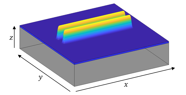
Figure 1: Schematic of two neighboring filaments (both indicated by the color gradient, with yellow representing maximum height) and thinner equilibrium film region (dark blue). The gray region represents the underlying SiO₂ substrate. In physical experiments [19], the in-plane dimensions are measured in hundreds of nm, typical metal thickness is 10-20 nm, and the substrate (membrane) thickness is on the order of 100 nm.

Consider a free surface metal filament of characteristic nanoscale thickness, $H=10$ nm, which we will use as a length scale. Suppose further that the metal is initially solid, exposed to air above, and in contact below with a thermally conductive solid SiO₂ substrate of depth $H_{\rm s}$, see Fig. 1. In order to develop a model, we make a number of simplifying assumptions, which we outline after presenting the model. Following [11], we choose the velocity scale $U=\gamma_{\rm f}/(3\mu_{\rm f})$ (where $\gamma_{\rm f}$ and $\mu_{\rm f}$ are surface tension and viscosity at melting temperature, $T_{\rm melt}$), leading to the time scale, $H/U$. Subsequently, we choose $T_{\rm melt}$, $\mu_{\rm f}U/H$ and $\gamma_{\rm f}$ as the temperature, pressure, and surface tension scales, respectively. We take the dimensionless domain length/width (in the $x$/$y$ directions) to be $P$.

Once in the liquid state, we treat the metal as an incompressible Newtonian fluid. The most complete model consists of the Navier-Stokes equations for the molten metal film, coupled with heat equations for the metal and substrate, plus appropriate boundary conditions and constitutive equations for the temperature-dependent material parameters. We assume that the viscosity depends on temperature, but that the surface tension, density, heat capacity and thermal conductivity of the material are fixed at their melting temperature values (see Sec. II of [18] for a justification of neglecting the temperature dependence of surface tension, and prior work [12] for discussion of the temperature dependence of thermal conductivity). Note in particular that the model allows for both spatial and temporal dependence of viscosity through the dependence of this material parameter on the temperature field. We use $T_{\rm f}$, $T_{\rm s}$ to denote the film and substrate temperatures, respectively and define $T_{\rm avg}(t)$, to be the time-dependent average filament temperature (see Sec. II of [18] for a complete definition). For the remainder of the text, we omit the argument of $T_{\rm avg}(t)$ with the understanding that it is time-dependent.

In recent work [11, 12] we proposed a simplified model for this setup based on a long-wave formulation for a thin metal geometry. The metal film thickness ($z=h(x,y,t)$ where $x$ and $y$ are the in-plane coordinates) evolution is governed by the following 4th order nonlinear partial differential equation,

$$\partial_{t}h+\nabla_{2}\cdot\left[\frac{1}{\mu(T_{\rm f})}h^{3}\nabla_{2}\left(\nabla_{2}^{2}h+\Pi(h)\right)\right]=0,\vspace{-0.1in}$$ (1)

where $\nabla_{2}=(\partial_{x},\partial_{y},0)$. Following the time derivative term in Eq. (1) are the capillary and disjoining pressure terms, respectively. Here, $\mu(T_{\rm f})$ represents temperature-dependent viscosity (scaled by $\mu_{\rm f}$), modeled via an Arrhenius-type relationship,

$$\mu(T_{\rm f})=S\left(T_{\rm f}\right)\exp\left(\mathcal{E}\left(\frac{1}{T_{\rm f}}-1\right)\right),$$ (2)

where $\mathcal{E}=E/(RT_{\rm melt})$ is related to the activation energy $E$ ($R$ is the universal gas constant)  [20]. This form also allows for melting/solidification control; the Sigmoid function $S\left(T_{\rm f}\right)=2\left(\tanh\left((T_{\rm f}-1)+\delta_{T}\right)+1\right)^{-1}$ approximates the phase transition ($\delta_{T}$ is set to $5{\rm K}/T_{\rm melt}$).

For metal films of nanoscale thickness, instability due to destabilizing metal-substrate interaction is an important effect since the range of the interaction potential is comparable to the film thickness [21]. This is modeled via a disjoining pressure of the form ${\Pi}({h})=\Omega[(h_{*}/h)^{n}-(h_{*}/h)^{m}]$, with equilibrium film thickness ${h}_{*}$, constant $\Omega$ (related to the Hamaker constant $A_{\rm H}$ by $\Omega={A_{\rm H}/{(6\pi\gamma_{\rm f}h_{*}^{3}H^{2})}}$), and exponents $n>m>1$ [22]. Such a disjoining pressure term ensures that the film height nowhere goes to zero, but instead approaches a minimum value comparable to $h_{*}$ as dewetting proceeds (we typically use $h_{*}=0.1$, corresponding to 1 nm; while this value is larger than that expected in experiments [23], this choice avoids the numerically more expensive simulations that are required for smaller values of $h_{*}$). Interfacial potentials for liquid metals are undoubtedly more complex than specified here, however, based on our earlier work and extensive comparison to experiment (see in particular [23]), we expect that the present form is sufficient for our purposes; further details on disjoining pressure models in this context are given in a recent review [10].

The heat flow model we developed recently [11] exploits further the long-wave approximation. The metal has much higher thermal conductivity than the substrate, and the temperature variation across the film (in the short, $z$-direction) may be shown to be weak. We retain those assumptions here, but different to our earlier work (and justified below), we assume that in-plane heat conduction in the substrate may be relevant and that heat is lost from the system only through the lateral substrate boundaries. This leads to the following system governing temperature,

$$h\mbox{Pe}_{\rm f}\partial_{t}T_{\rm f} =\nabla_{2}\cdot\left(h\nabla_{2}T_{\rm f}\right)-\mathcal{K}\partial_{z}T_{\rm s}|_{z=0}+h\overline{Q},$$ (3)

$$\mbox{Pe}_{\rm s}\partial_{t}T_{\rm s} =\nabla_{2}^{2}T_{\rm s}+\partial_{z}^{2}T_{\rm s},$$ (4)

for $z\in\left(0,h\right)$ and $z\in\left(-H_{s},0\right)$, respectively. The boundary conditions (BCs) include continuity of temperature at $z=0$ and appropriate BCs at the domain boundaries: $T_{\rm f}=T_{\rm s}$ at $z=0$, $\partial_{z}T_{\rm s}=0$ at $z=-H_{s}$, $\partial_{x}T_{\rm f}=0$ at $x=0,P$, $\partial_{y}T_{\rm f}=0$ at $y=0,P$, and $T_{\rm s}=T_{\rm a}$ (ambient temperature) at $x=0,P$, $y=0,P$. The parameters, defined by

$$\mbox{Pe}_{\rm f} =\frac{\left(\rho c\right)_{\rm f}UH}{k_{\rm f}},\qquad\mbox{Pe}_{\rm s}=\frac{\left(\rho c\right)_{\rm s}UH}{k_{\rm s}},\qquad\mathcal{K}=\frac{k_{\rm s}}{k_{\rm f}},$$

represent the film and substrate Peclet numbers, and thermal conductivity ratio, respectively. Equation (3) describes the leading order fluid temperature and the terms on the right-hand side represent the in-plane diffusion, heat loss due to the substrate, and heat generated due to the laser, averaged over the metal thickness,

$$\overline{Q}=\frac{A(h)}{h}\int_{0}^{h}F(t)\left[1-R(h)\right]\exp\left[-\alpha_{\rm f}\left(h-z\right)\right]dz.$$ (5)

Here, $\alpha_{\rm f}^{-1}$ is the absorption length for laser radiation in the metal film and $F(t)$ captures the temporal shape of the laser pulse, taken to be Gaussian centered at specified time $t_{\rm p}$ and of prescribed width $\sigma$ (corresponding to tens of nanoseconds). The term $A(h)$ is a smooth approximation of $\mathcal{U}(h-h_{*})$, the unit step function centered at $h_{*}$, which turns off absorption as $h\rightarrow h_{*}$. In-plane diffusion is similarly turned off as $h\rightarrow h_{*}$, which ensures that the filaments alone absorb energy and transfer heat to other filaments only via the substrate. In general, the reflectivity of the film on a transparent substrate, $R(h)$, is found by solving Maxwell’s equations [24], but the resultant form is cumbersome; following earlier work [25, 13] we approximate it by $R(h)=r_{0}\left(1-\exp\left(-\alpha_{\rm r}{h}\right)\right)$, where $r_{0}$ and $\alpha_{\rm r}$ are parameters, chosen to ensure good agreement with the exact solution.

Equation (4) describes the substrate heat conduction. The BCs on Eqs. (3) and (4) impose no heat loss at the bottom of the substrate (motivated by the experiments on thin substrates (membranes) discussed below), as well as insulating conditions for the metal at its lateral boundaries. We impose room temperature at the lateral boundaries of the substrate, leading to the only heat loss mechanism. The no-heat loss BC at the bottom of the substrate motivates the inclusion of in-plane thermal flow in Eq. (4) since there is no significant heat flow in the $z$ direction.

In deriving our model, we made the following additional assumptions not yet discussed: (i) inertial effects are negligible (discussed and justified elsewhere [26]); (ii) phase change (melting, solidification) is fast, and the associated energy gain/loss can be ignored (see e.g. [25, 13]); (iii) heat is lost from the metal only through the substrate with no radiative losses [12]; (iv) the metal does not evaporate. We also reiterate that the equilibrium layer of thickness $h_{*}$ plays no role in thermal transport; we remove heat diffusion (the first term on the right-hand side of Eq. (3)) through this layer to reduce its role to modeling fluid-dynamical aspects of the problem only.

Results

We focus on setups relevant to recent experiments [27] involving nanoparticle formation on so-called ‘membranes’. Membranes are essentially very thin solid substrates with overlaid nanoscale metal patterns, obtained by combining lithographic techniques with chemical etching of the underlying silicon [27]. An important motivation for using membranes is that one is able to observe not only the final outcome of the experiments but also the time evolution since membranes are optically transparent and allow for the use of dynamic transmission electron microscopy (DTEM), which provides unique nanosecond temporal and nanometer spatial resolution [27]. From the modeling perspective, the key point is that the Biot number is typically very small so the bottom boundary of the substrate is essentially insulating. Therefore, the membrane setup allows for precise control of heat flow. We note that, while carrying out experiments on (thick) SiO₂ wafers requires more energy, the model that we have discussed here describes such experiments accurately as well, see [12] for details.

In our simulations, the initial condition is a metal filament, possibly surrounded by other filaments at a specified distance apart, with the exact geometry specified in Sec. I of [18]. Initially, both metal and substrate are at room temperature. Then, the laser pulse is applied, the metal temperature increases (discussed more precisely in what follows), and when the filament temperature rises above the melting point, it starts evolving as a Newtonian fluid. When the laser energy begins to decrease, the filament temperature decreases as well, and once it drops below the melting temperature, the evolution stops. The simulations are carried out using our in-house GPU-based code [17]. The computational method itself is based on finite difference spatial discretization, combined with Crank-Nicolson temporal evolution within an ADI (alternate direction implicit) framework; see [12] for details. The parameters used in all simulations are provided in Table 1 of [18].

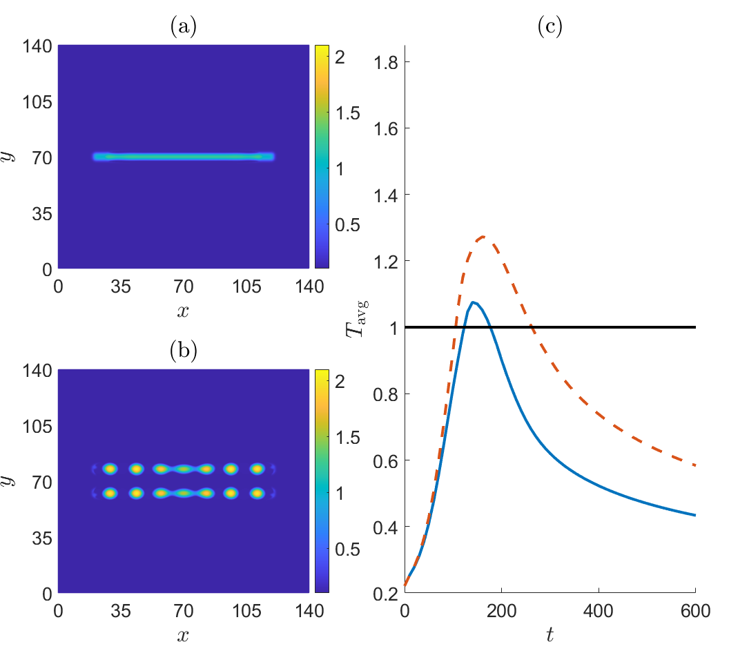
Figure 2: Final configuration of (a) a single metal filament and (b) two metal filaments placed at a distance of $D=15$ apart, exposed to the same laser pulse. Frame (c) shows the maximum temperatures for the configurations in (a) ( blue solid line) and (b) ( red dashed line), along with the melting line (black). See also Animation 1 [28] for fluid evolution and temperature fields.

Figure 2(a - b) shows the results of two sets of simulations, whose only difference is the number of filaments present. Still, the final outcome is very different. While in both cases the filament melts, no significant instability development has occurred in (a) prior to resolidification, whereas in (b) the evolution is much more advanced, exhibiting a pearling type of instability [29, 30]. Figure 2(c) shows why: the average temperature is significantly higher in the case of two filaments, and furthermore, the metal temperature in this case remains above melting for a longer time. Due to the Arrhenius-type dependence of viscosity on temperature, the evolution is also faster when multiple filaments are present. Animation 1 [28] shows the time- and space-dependence of the film and temperature evolution; note that filaments cool faster towards their ends. The animation also emphasizes the significantly higher temperature attained for two filaments compared to one, leading to the faster evolution and breakup noted above. We remark that the details of the final outcome depend on the choice of parameters, including the filaments’ volume and aspect ratio, see Secs. V and VI of [18]; the concept of thermal crowding is, however, always found to hold, with faster evolution and breakup for multiple filaments.

Figure 3 shows the effect that the number of filaments and their respective spacing has on the collective heating and dewetting, illustrating that thermal crowding can strongly influence filament evolution. The comparison of different rows shows that an increase in the number of filaments strongly influences their temperatures and, through the temperature-dependent viscosity, the resultant dewetting. For example, in Fig. 3(b) the filaments melt but not sufficiently even to dewet partially, whereas the filaments in Fig. 3(e, h) both show full dewetting of the interior filaments. Interestingly, the filaments that are farthest from the center only begin undulation growth before they freeze in place because they only receive one-sided diffusive heating from the other filaments. The interior filaments of Fig. 3(e, h) then spend more time in the liquid phase, are hotter, of lower viscosity, and therefore evolve faster than the outermost filaments; see also Animation 2 [28]. This animation also illustrates the relevance of both the number of filaments and their spacing; in the particular case considered here, the distance between filaments is more important since the configuration in Fig. 3(d) (three filaments at spacing $D=15$) remains hot longer than that in Fig. 3(h) (four filaments at spacing $D=20$), consistent with the information on average temperatures provided by Fig. 3(j, k).

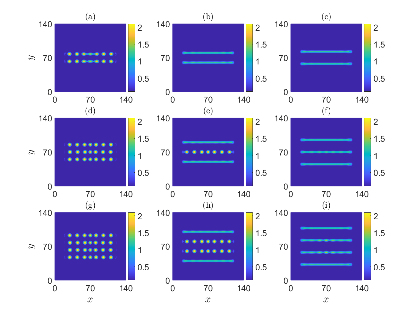
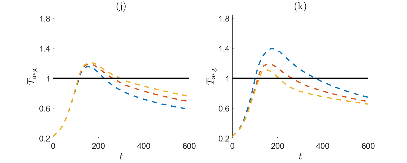
Figure 3: (a-i) Final configuration of two (row 1), three (row 2), and four filaments (row 3) at distances $D=15$ (column 1), $D=20$ (column 2), $D=25$ (column 3). (j) Time evolution of the average film temperature for (b) blue dashed line, (e) orange dashed line, and (h) yellow dashed line. (k) Time evolution of the average film temperature for (d) blue dashed line, (e) orange dashed line and (f) yellow dashed line. The melting temperature, $T_{\rm melt}$, is shown by the solid black line. See also Animations 2 and 3 at [28].

In principle, there are two possible reasons for the unbalanced heating leading to a breakup of internal filaments only: (i) loss of heat through the domain boundaries, and also (ii) decreased heating of the external filaments by the internal ones. Insight regarding which of these two mechanisms is most relevant can be reached by carrying out simulations on larger domains. These additional results, see Sec. IV of [18], show that the influence of the heat loss through domain boundaries is minimal, and therefore, one-sided heating governs the evolution and breakup.

Figure 3(j) shows that increasing the number of filaments, while keeping their spacing fixed, has a fairly modest effect on the maximum metal temperature, but a larger number of filaments collectively retains heat for longer, leading to increased liquid lifetimes and more complete dewetting in the cases with three and four filaments. Figure 3(k) shows that increasing the inter-filament distance, $D$, leads to lower filament temperatures. In particular, placing three filaments at a distance $D=15$ (Fig. 3(d)) is sufficient to collectively melt and fully evolve all three into nanoparticles, as opposed to placing them at distance $D=25$ (Fig. 3(f)), which (although the filaments melt) is insufficient to produce any nanoparticle formation. Additional information regarding spatial temperature distribution is available in Animation 3, which shows that the temperature maxima occur at the center of the domain, with lower temperatures towards the periphery, consistent with, e.g., the results shown in Fig. 3(i) where for the central filaments, we observe better-developed undulations towards the filament centers.

Figure 4 illustrates that filament instability can be initiated asymmetrically. Here, we place short filaments on both sides of the long filament that was shown in Fig. 2(a), which alone does not break up. The presence of the additional short filaments is, however, sufficient to increase the temperature of the left side of the long filament and induce breakup. The short filaments themselves melt; however, asymmetric one-sided heating is insufficient for their complete breakup. Additionally, Animation 4 [28] shows that the leftmost droplet solidifies prior to fully dewetting, illustrating the nontrivial competition between the edge retraction and the resolidification. Additional examples of more elaborate filament configurations are given in Sec. VII of [18].

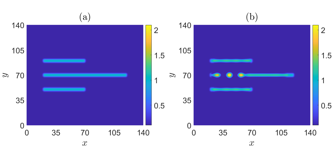
Figure 4: Initial (a) and final (b)configuration for asymmetric setup with a filament of length $100$ surrounded by two filaments of length $50$ placed at a distance $D=20$. See also Animation 4 at [28].

Conclusions

We have illustrated a simple but powerful method that allows for the coupling of fluid dynamics and heat transport for metal filaments deposited on thermally conductive substrates. Our approach is fully self-consistent, with fluid dynamics influencing and being influenced by the heat flow. This coupling occurs through temperature dependence of metal viscosity, whose spatial variation influences the fluid thickness and, in turn, affects the amount of heating absorbed. In the present work, we apply this method to metal filaments; however, the model can be used for any material and any initial material geometry exposed to volumetric heating. In the context of metals, our results open the door to various directed- and self-assembly approaches since it is now possible to control the dynamics simply by specifying the initial material distribution.

References

- Grzelczak et al. [2010] M. Grzelczak, J. Vermant, E. M. Furst, and L. M. Liz-Marzán, Directed self-assembly of nanoparticles, ACS Nano 4, 3591 (2010).
- Chai et al. [2022] Z. Chai, A. Childress, and A. A. Busnaina, Directed assembly of nanomaterials for making nanoscale devices and structures: Mechanisms and applications (2022).
- Atwater and Polman [2010] H. Atwater and A. Polman, Plasmonics for improved photovoltaic devices, Nature Materials 9, 9 (2010).
- Wang and Li [2011] D. Wang and Y. Li, Bimetallic nanocrystals: Liquid-phase synthesis and catalytic applications, Advanced Materials 23, 1044 (2011).
- Chaudhuri and Paria [2012] R. G. Chaudhuri and S. Paria, Core/shell nanoparticles: Classes, properties, synthesis mechanisms, characterization, and applications, Chemical Reviews 112, 2373 (2012).
- Makarov et al. [2016] S. V. Makarov, V. A. Milichko, I. S. Mukhin, I. I. Shishkin, D. A. Zuev, A. M. Mozharov, A. E. Krasnok, and P. A. Belov, Controllable femtosecond laser-induced dewetting for plasmonic applications, Laser Photonics Rev. 10, 91 (2016).
- Hughes et al. [2017] R. A. Hughes, E. Menumerov, and S. Neretina, When lithography meets self-assembly: a review of recent advances in the directed assembly of complex metal nanostructures on planar and textured surfaces, Nanotechnology 28, 282002 (2017).
- Ruffino and Grimaldi [2019] F. Ruffino and M. G. Grimaldi, Nanostructuration of thin metal films by pulsed laser irradiations: A review, Nanomaterials 9, 1133 (2019).
- Fowlkes et al. [2011] J. D. Fowlkes, L. Kondic, J. A. Diez, and P. D. Rack, Self-assembly versus directed assembly of nanoparticles via pulsed laser induced dewetting of patterned metal films, Nano Letters 11, 2478 (2011).
- Kondic et al. [2020] L. Kondic, A. G. González, J. A. Diez, J. D. Fowlkes, and P. Rack, Liquid-state dewetting of pulsed-laser-heated nanoscale metal films and other geometries, Annu. Rev. Fluid Mech. 52, 235 (2020).
- Allaire et al. [2021] R. H. Allaire, L. J. Cummings, and L. Kondic, On efficient asymptotic modelling of thin films on thermally conductive substrates, J. Fluid Mech. 915, A133 (2021).
- Allaire et al. [2022] R. H. Allaire, L. J. Cummings, and L. Kondic, Influence of thermal effects on the breakup of thin films of nanometric thickness, Phys. Rev. Fluids 7, 064001 (2022).
- Trice et al. [2007] J. Trice, D. Thomas, C. Favazza, R. Sureshkumar, and R. Kalyanaraman, Pulsed-laser-induced dewetting in nanoscopic metal films: Theory and experiments, Phys. Rev. B 75, 235439 (2007).
- Atena and Khenner [2009] A. Atena and M. Khenner, Thermocapillary effects in driven dewetting and self assembly of pulsed-laser-irradiated metallic films, Phys. Rev. B 80, 075402 (2009).
- Saeki et al. [2013] F. Saeki, S. Fukui, and H. Matsuoka, Thermocapillary instability of irradiated transparent liquid films on absorbing solid substrates, Phys. Fluids 25 (2013).
- Shklyaev et al. [2012] S. Shklyaev, A. A. Alabuzhev, and M. Khenner, Long-wave marangoni convection in a thin film heated from below, Phys. Rev. E 85, 016328 (2012).
- Allaire [2021] R. H. Allaire, Gadit thermal, https://github.com/Ryallaire/GADIT_THERMAL (2021).
- sup [a] (a), see Supplemental Material at [URL will be inserted by publisher].
- McKeown et al. [2012] J. T. McKeown, N. A. Roberts, J. D. Fowlkes, Y. Wu, T. LaGrange, B. W. Reed, G. H. Campbell, and P. D. Rack, Real-time observation of nanosecond liquid-phase assembly of nickel nanoparticles via pulsed-laser heating, Langmuir 28, 17168 (2012).
- Gale and Totemeier [2004] W. Gale and T. Totemeier, Smithells Metals Reference Book (Eighth Edition) (Butterworth-Heinemann, 2004).
- Israelachvili [1992] J. N. Israelachvili, Intermolecular and surface forces (Academic Press, New York, 1992) second edition.
- Dong and Kondic [2016] N. Dong and L. Kondic, Instability of nanometric fluid films on a thermally conductive substrate, Phys. Rev. Fluids 1, 063901 (2016).
- González et al. [2013] A. González, J. A. Diez, Y. Wu, J. D. Fowlkes, P. D. Rack, and L. Kondic, Instability of liquid Cu films on a SiO2 substrate, Langmuir 29, 9378 (2013).
- Heavens [1955] O. Heavens, Optical Properties of Thin Solid Films, Dover books on physics and mathematical physics (Dover Publications, 1955).
- Seric et al. [2018] I. Seric, S. Afkhami, and L. Kondic, Influence of thermal effects on stability of nanoscale films and filaments on thermally conductive substrates, Phys. Fluids 30, 012109 (2018).
- González et al. [2016] A. G. González, J. A. Diez, and M. Sellier, Inertial and dimensional effects on the instability of a thin film, J. Fluid Mech. 787, 449 (2016).
- Diez et al. [2021] J. Diez, A. González, D. Garfinkel, P. Rack, J. McKeown, and L. Kondic, Simultaneous decomposition and dewetting of nanoscale alloys: A comparison of experiment and theory, Langmuir 37, 2575 (2021).
- sup [b] (b), see Supplemental Material at [URL will be inserted by publisher] for animations.
- Diez and Kondic [2007] J. A. Diez and L. Kondic, On the breakup of fluid films of finite and infinite extent, Phys. Fluids 19, 072107 (2007).
- Diez et al. [2009] J. A. Diez, A. González, and L. Kondic, On the breakup of fluid rivulets, Phys. Fluids 21, 082105 (2009).