On the Origin of Llamas: Model Tree Heritage Recovery

Abstract

The rapid growth of neural network models shared on the internet has made model weights an important data modality. However, this information is underutilized as the weights are uninterpretable, and publicly available models are disorganized. Inspired by Darwin’s tree of life, we define the Model Tree which describes the origin of models i.e., the parent model that was used to fine-tune the target model. Similarly to the natural world, the tree structure is unknown. In this paper, we introduce the task of Model Tree Heritage Recovery (MoTHer Recovery) for discovering Model Trees in the ever-growing universe of neural networks. Our hypothesis is that model weights encode this information, the challenge is to decode the underlying tree structure given the weights. Beyond the immediate application of model authorship attribution, MoTHer recovery holds exciting long-term applications akin to indexing the internet by search engines. Practically, for each pair of models, this task requires: i) determining if they are related, and ii) establishing the direction of the relationship. We find that certain distributional properties of the weights evolve monotonically during training, which enables us to classify the relationship between two given models. MoTHer recovery reconstructs entire model hierarchies, represented by a directed tree, where a parent model gives rise to multiple child models through additional training. Our approach successfully reconstructs complex Model Trees, as well as the structure of “in-the-wild” model families such as Llama 2 and Stable Diffusion.

1 Introduction

page

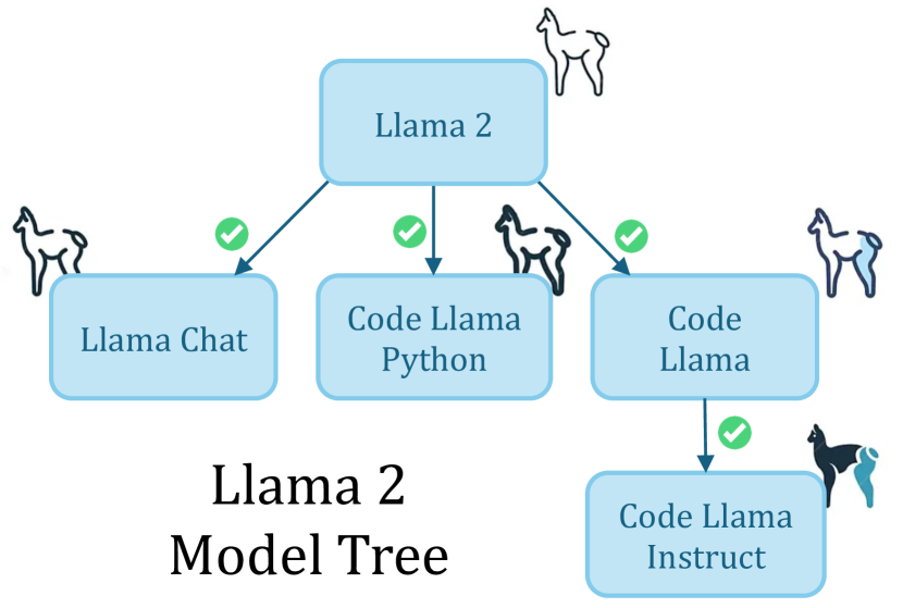
Figure 1: Llama2 Model Tree: We perform MoTHer Recovery in-the-wild, successfully recovering the Llama2 Model Tree with perfect accuracypage

The number and diversity of neural models shared online have been growing at an unprecedented rate, establishing model weights as an important data modality (12; 6; 26; 19). On the popular model repository Hugging Face alone there are over 600,000 models, with thousands more added daily. Many of these models are related through a common ancestor (i.e., foundation model) from which they were fine-tuned. We hypothesize that the model weights may encode this relationship. Motivated by Darwin’s tree of life (7), which describes the relationships between organisms, we analogously define the Model Tree to describe the hereditary relations between models. Reminiscent of the natural world, the structure of the Model Tree is unknown. We therefore propose the task of Model Tree Heritage Recovery (MoTHer Recovery) for mapping Model Trees in the rapidly evolving universe of neural networks.

Recovering the Model Tree is important for several reasons. First, it establishes the lineage of a model, determining whether one model originated from another (i.e., via fine-tuning). This can help resolve legal disputes over model authorship or wrongful use of proprietary training data. For instance, a foundation model may be trained on proprietary data and publicly released. By using the graph combined with membership inference attacks (32), one could identify fine-tuned versions of the model and take appropriate action. In the long term, mapping the model universe represents an exciting field of research, akin to how search engines index the internet (2).

We begin our exploration of the Model Tree by studying the relationship between the weights of related models. Our main finding is that outlier values in the weights of related models often indicate their relationship. We find that the distance between these outliers correlates with their node distance on their family tree. We then proceed to examine how the weights of a model evolve over the course of training. We observe that the number of weight outliers changes monotonically over the course of training. Specifically, we distinguish between a generalization stage (often called pre-training) and a specialization stage (often referred to as fine-tuning). We find that during generalization, the number of weight outliers grows, while during specialization, it diminishes.

With these observations, we attempt to recover a Model Tree for a set of models. This requires determining whether each pair of models is directly connected and establishing the direction of the relationship. We use the outlier-based distance to create a pairwise distance matrix and the outlier monotonicity to create a binary edge direction matrix. Finally, we use a minimum directed spanning tree algorithm on the combined distance matrix to recover our Model Tree. We extend the Model Tree to a Model Graph, allowing us to recover ecosystems with multiple trees by first clustering the nodes based on their pairwise distances.

We demonstrate the efficacy of our method on a curated dataset as well as real-world ecosystems such as the Llama 2 family (33; 30) and the Stable Diffusion family (29). We extensively ablate our method, justifying our technical choices. Finally, we discuss a way forward towards recovering Model Graphs at web scale such as the Hugging Face Model Graph.

To summarize, our main contributions are:

1. Proposing the Model Tree and Model Graph data structures for describing the hereditary relations between models.

2. Uncovering the connection between model weight outlier values and their distance on the Model Graph.

3. Introducing the task of Model Tree Heritage Recovery and demonstrating the effectiveness of MoTHer recovery in real-world scenarios.

2 Related Works

page

Model weight processing.

Although model weights fully characterize the capabilities of the model, most research is focused on model activations (4; 31; 41; 9). Early works (14; 15; 1) visualized the trajectory of weights using principled component analysis (PCA). Eilertsen et al. (11) performed a large empirical study of model weights, representing each model as a point in the neural weight space and training classifiers to predict different training hyper-parameters. The seminal work of (24) proposed using a HyperNet to generate parameters of a model, recent works (12; 39; 36; 28) used diffusion models to generate the weights of small networks. More recently, a line of works predict model aspects performance or classify models based on their weights by projecting the weight into an embedding space (21; 6) or by incorporating permutation invariance priors while training a neural network on the weights (40; 23; 25; 27; 26; 34). Recently, Horwitz et al. (19) demonstrated a vulnerability wherein the weights of a pre-trained model can be recovered using a small number of LoRA fine-tuned models. Overall, model weight processing remains an underexplored area that is poised to grow in the coming years.

3 The Model Graph

page

Definition.

We introduce the Model Tree, a data structure for describing the origin of models stemming from a base model (e.g., a foundation model). Consider a set of models $\mathcal{V}$, where the base model $v_{b}\in\mathcal{V}$ serves as the root node. Every model $v\in\mathcal{V}\setminus\{v_{b}\}$, is fine-tuned from another model. We refer to the model from which $v$ was fine-tuned as its parent model, and denote it by $Pa(v)$. Conversely, we refer to $v$ as a child of $Pa(v)$. A parent can have multiple children (including none), while all models except the root have only one parent. The set of tree edges is denoted by $\mathcal{E}$, where each directed edge between a parent and its child is represented as $e=(Pa(v),v)$. Overall, the Model Tree $\mathcal{T}$ is defined by its nodes and directed edges, $\mathcal{T}=(\mathcal{V},\mathcal{E})$. We denote by $d(u,v)$ the number of edges on the shortest path in $\mathcal{T}_{+}$ between the nodes $u$ and $v$. The tree $\mathcal{T}_{+}$ is the same as our tree $\mathcal{T}$ except that the directed edges are replaced by undirected ones.

A collection of Model Trees $\mathcal{T}_{1},\ldots,\mathcal{T}_{n}$ forms a forest, which we call a Model Graph. This Model Graph is defined as $\mathcal{G}=(\mathcal{V}=\mathcal{V}_{1}\cup\ldots\cup\mathcal{V}_{n},\mathcal{E}=\mathcal{E}_{1}\cup\ldots\cup\mathcal{E}_{n})$. In a Model Graph, $d(u,v)$ is only defined if $u,v\in\mathcal{T}_{i}$, when $u\in\mathcal{T}_{i}$ and $v\in\mathcal{T}_{j}$, $d(u,v)$ is undefined. As the architecture of a model is given by its weights, and since different architectures necessarily belong to different trees, we can assume without loss of generality that all $v\in\mathcal{V}$ are of the same architecture.

Task definition.

Due to the large number and diversity of models, the structure of the Model Graph is unknown and is non-trivial to estimate. We therefore introduce the task of Model Tree Heritage Recovery (MoTHer Recovery) for mapping the structure of the Model Graph.

Formally, given a set of models $\mathcal{V}$, the goal is to recover the structure of the Model Graph $\mathcal{G}=(\mathcal{V},\mathcal{E})$ based solely on the weights of the models $v\in\mathcal{V}$. Since a Model Graph is a forest of Model Trees, the task involves two main steps: (i) Cluster the nodes into different components $\mathcal{T}_{1},\mathcal{T}_{2},\ldots$, where each component is a Model Tree with an unknown structure. (ii) Recover the structure of each Model Tree $\mathcal{T}_{i}$. Essentially, as each graph is defined by its vertices and edges, the task is to recover the directed edges $\mathcal{E}$ using the weights of $v\in\mathcal{V}$.

4 Model Graph Priors

page

Figure 2: Weight Distance vs. Model Tree Edge Distance: Our weight distances $\ell_{FT}$ and $\ell_{LoRA}$ almost perfectly correlate with the number of edges between models in a Model Tree. Thus is a good indicator for determining parent-child relation, i.e., models that were fine-tuned from one anotherpage

Despite the recent growth in public models, and although model weights fully characterize the behavior of a model, model weights remain largely uninterpretable. Here, we explore two key properties of model weights that enable Model Graph recovery. In sec:recovering, we utilize these properties for our method, MoTHer Recovery.

4.1 Estimating node distance from model weights

page

In this section, we investigate the use of model weights to predict the distance between two models in the Model Tree. This will help us determine whether two models are related via an edge.

First, we define the weight distance between models. Let $u$ and $v$ be two models, and $u_{l}$ and $v_{l}$ denote the weight matrix of layer $l$ of models $u$ and $v$ respectively,

$$\cref@constructprefix{page}{\cref@result}\ell_{FT}(u,v)=\max_{l\in L}(\max(u_{l}-v_{l}))$$ (1)

where $L$ is a set of model layers.

Next, we study the weight distance $\ell_{FT}(u,v)$ between pairs of models as a function of the edge distance $d(u,v)$ between their respective nodes on the Model Tree. In fig:node_distance_analysis, we plot the relationship between these two distances ($\rho=0.99$). It is evident that nodes with direct parent-child connections (i.e., models fine-tuned from one another) have the lowest weight distance. We conclude that a low $\ell_{FT}$ distance between two models is highly correlated with an edge between their nodes and vice versa. Note that we use “distance” in a colloquial sense, as mathematically it does not satisfy the definitions of a distance.

LoRA fine-tuning.

LoRA (20) has become the dominant method for parameter-efficient fine-tuning. When fine-tuning a model via LoRA, the entire model is frozen, and only a subset of the layers tune a new low-rank matrix for each layer. Consequently, a model fine-tuned via rank $r$ LoRA differs from its base model by a matrix of at most rank $r$ for each layer. Furthermore, two models fine-tuned from the same base model using rank $r_{1}$ and $r_{2}$ LoRAs differ from each other by a matrix of at most rank $r_{1}+r_{2}$ per layer. We use this property to provide a better estimate of the node distance between LoRA models and define the LoRA weight distance as:

$$\cref@constructprefix{page}{\cref@result}\ell_{LoRA}(u,v)=\max_{l\in L}\left(rank(u_{l}-v_{l})\right)$$ (2)

where $L$ is the set of fine-tuned LoRA weights. In practice, we compute the rank using singular value decomposition (SVD), where the rank is the number of singular values greater than some threshold $\epsilon$. Similar to the full fine-tuning case (see fig:node_distance_analysis), a low LoRA weight distance between two models is highly correlated with an edge between their nodes.

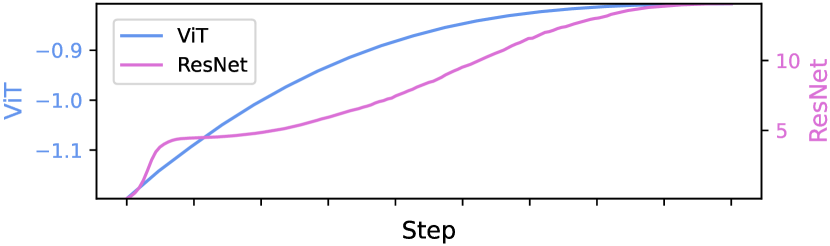
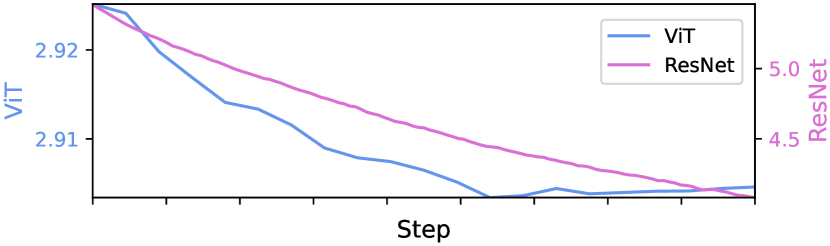
Figure 3: Directional Weight Score: We plot the change in the directional weight score throughout the pre-training (generalization) stage (left) and fine-tuning (specialization) stage (right). In all cases, the directional score is almost monotonic, indicating the increasing number of weight outlier values during generalization and the decreasing number during specialization. The ResNet (18) and ViT(8) models were pre-trained and fine-tuned independently at each stagepage

4.2 Estimating edge direction from weights

page The direction of an edge between two nodes $u$ and $v$ reflects whether model $v$ was trained from $u$ or vice versa. The weight distance from sec:node_dist_prior cannot disentangle the direction as it results in a symmetric matrix. Estimating the direction of edges requires a statistic of the weights that evolve monotonically during training. To this end, we use kurtosis (i.e., fourth moment) and define the directional weight score as:

$$\cref@constructprefix{page}{\cref@result}k(u)=\sum_{l\in L}\frac{E\left[\left(u_{l}-\mu\right)^{4}\right]}{\left(E\left[\left(u_{l}-\mu\right)^{2}\right]\right)^{2}}$$ (3)

where $L$ is a set of model layers. Note that the directional score only defines an order between related nodes; unrelated nodes may have very different scores.

To study the effectiveness of this score, we observe how the weights of a model evolve throughout the training process. Interestingly, we found that the training process can be categorized into two stages: a generalization stage and a specialization stage. As seen in fig:gen_spec_intuition, while the score is monotonic in both stages, it increases during generalization and decreases during specialization. Although generalization is usually attributed to pre-training and specialization to fine-tuning, this is not necessarily always the case. The term fine-tuning is typically used for any training performed after the initial pre-training stage. However, generalization training may also be applied to an already pre-trained model, we show such an example in sec:experiments (Stable Diffusion).

Intuition.

Consider a model with Gaussian-based weight initialization, such as Kaiming initialization by He et al. (17). During the generalization stage, to better encode large, general-purpose datasets, the weights of a model will likely require an increasing number of diverse values. This may lead to an increase in the number of outlier values in the weight matrix. In contrast, during the specialization stage, the weights of a model with a lower value diversity will likely suffice to encompass the smaller, task-specific data. This may lead to a decrease in the number of outlier values in the weight matrix. Kurtosis, as a measure of the “tailedness” of a distribution, captures this property.

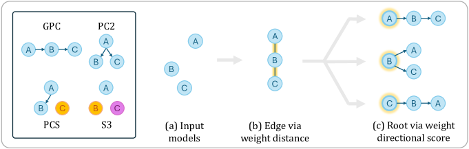
Figure 4: Recovering a Simplified Model Graph: We enumerate all possible Model Graphs of size $3$ (left). On the right, we demonstrate a Model Graph Recovery process. (a) A set of $3$ models with no prior knowledge regarding their relations. (b) Place edges between the nodes with the lowest weight distance. (c) Designate the node with the highest directional weight score as the rootpage

5 Model Tree Heritage Recovery

page Given the above priors, we now describe how to recover the structure of Model Graphs. As a warm-up problem, in sec:warm_up we start by manually solving all the $3$ nodes Model Graphs. Then, in sec:scaling we describe MoTHer, our proposed algorithm for recovering real Model Graphs.

In both cases, we have access to the model weights and assume that we are given the training stage of each node (i.e., generalization or specialization). Each Model Graph may contain one or more Model Trees. Connected nodes within a Model Tree are derived from each other via additional training steps. Unless otherwise specified, we assume no prior knowledge regarding the model relations.

5.1 Warm-up: A simplified Model Graph

page To recover a Model Graph of size $3$, we place edges between the nodes with the lowest weight distance and designate the node with the highest directional weight score as the root. Next, we elaborate on each of the possible size $3$ Model Graphs.

Grandparent-Parent-Child (GPC).

This Model Tree exhibits a $3$-generational relationship, where each node is derived from the previous one (see fig:basic_alg). To recover the underlying Model Tree structure, we use $\ell_{FT}$ to place edges between node pairs with the lowest weight distances. This is motivated by our analysis in sec:node_dist_prior,fig:node_distance_analysis. Next, to determine the order of the nodes, we use the directional score shown in eq:kurtosis and designate the node with the highest score as the root. Combining these steps fully constructs the GPC Model Tree, we illustrate this process in fig:basic_alg. Note that the above process assumes the specialization training stages for all $3$ models. To adjust the process for the generalization stage, simply change the sign of the directional score. When the training stages of each node differ, we choose the sign of the directional score according to each node’s training stage.

Parent-Child-Child (PC2).

This Model Tree contains one parent with two children (see fig:basic_alg). As in the GPC case, we start by placing the edges using the weight distance defined in eq:mother_distance_full_ft. Since both children are derived from the root, the directional score will predict the node with the highest score as the root (see fig:basic_alg). Different training stages are handled as in the GPC case.

Parent-Child-Stranger (PCS).

Unlike the previous triplets, here we have a Model Graph comprised of two Model Trees (see fig:basic_alg). To recover this structure, we first identify the node with no edge according to the pairwise weight distance. Since that node belongs to a different Model Tree, it will have a larger distance than a set threshold, allowing us to classify it as the odd one. With the node isolated, we can follow the protocol of the previous Model Trees for the two remaining nodes.

Stranger-Stranger-Stranger (S3).

Finally, here we have a Model Graph comprising $3$ Model Trees (see fig:basic_alg). Similar to PCS, we can cluster them into different Model Trees based on their large distances, allowing us to identify the structure.

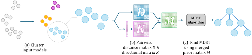
Figure 5: MoTHer Recovery Overview: Our proposed Model Graphs and Model Trees are new data structures for describing the heredity training relations between models. In these structures, heredity relations are represented as directed edges. We introduce the task of MoTHer Recovery its goal is to uncover the unknown structure of Model Graphs based on the weights of a set of input models. Our algorithm works as follows: (a) Cluster into different Model Trees based on the pairwise weight distances. (b) For each cluster, i) use $\ell_{FT}$ or $\ell_{LoRA}$ to create a pairwise distance matrix $D$ for placing edges, and ii) create a binary directional matrix $K$ based on the kurtosis to determine the edge direction. (c) To recover the final Model Tree, run a minimum directed spanning tree (MDST) algorithm on the merged prior matrix $M$. The final recovered Model Graph is the union of the recovered Model Treespage

5.2 MoTHer Recovery: Scaling up Model Graph Recovery

page We present MoTHer, our method for recovering the structure of larger Model Graphs. Let $v_{1},\ldots,v_{n}\in\mathcal{V}$ be a set of nodes representing different models that share the same architecture. For simplicity, assume for now that all $v_{1},\ldots,v_{n}\in\mathcal{T}$ , i.e., all nodes are from the same Model Tree, we will later relax this assumption.

Our goal is to recover the edges $\mathcal{E}$ of the Model Tree $\mathcal{T}$, this is done by placing edges between two nodes, where one was trained from the other. As seen above, recovering the structure requires a combination of the estimated weight distance and the edge direction. Let $D$ be a weight distance matrix and let $K$ be a binary directional matrix,

$$D_{ij} =\begin{cases}\ell(v_{i},v_{j}),&\text{if }i\neq j\\ \infty,&\text{otherwise}\end{cases}, \quad K_{ij} =\begin{cases}1,&\text{if }k(v_{i})<k(v_{j})\\ 0,&\text{otherwise}\end{cases}$$ (4)

To allow for both generalization and specialization node relations, we define $T$ as a binary matrix

$$T_{ij}=\begin{cases}1,&\text{if generalization}\\ 0,&\text{otherwise}\end{cases}$$ (5)

The final distance matrix for recovering the Model Tree takes into account all $3$ constraints as follows,

$$M_{ij} =D+\lambda(K\oplus T)$$ (6)

where $\oplus$ is a binary XOR and $\lambda$ regularizes the directional score, allowing for some mistakes. Since $\ell_{FT}$ and $\ell_{LoRA}$ may range in value, we define $\lambda$ to be proportional to $D$ with $\lambda=c\cdot(\frac{1}{n^{2}}\sum_{i,j=1}^{n}{D_{ij}})$ where $c$ is some constant.

We can recover the Model Tree from $M$ using a minimum directed spanning tree (MDST) algorithm. In this paper, we employ the Chu-Liu-Edmonds’ algorithm (5; 10), which iteratively contracts cycles in the graph until forming a tree. The algorithm proceeds as follows: initially, it treats each node as a temporary tree. Then, it merges the temporary trees via the incoming edge with the minimum weight. Subsequently, it identifies cycles in the remaining temporary trees and removes the edge with the highest weight. This merging process continues until all cycles are eliminated, resulting in the minimum directed spanning tree. The algorithm runs in $O(EV)$, however, faster MDST algorithms exist (13) with $O(E+VlogV)$.

Multiple components.

Thus far we assumed all $v_{1},\ldots,v_{n}$ are from the same tree. To relax this assumption we add an additional clustering step before running the above algorithm. Specifically, we run a clustering algorithm on the pairwise $L_{1}$ distance of $v_{1},\ldots,v_{n}$ and find the MDST for each of the clusters independently.

6 Experiments

page

Experimental setup

To evaluate the performance of MoTHer we construct the ViT Tree Heritage Recovery (VTHR) dataset containing $3$ splits: i) FT: full fine-tuning, ii) LoRA-V: LoRA fine-tuning with varying ranks, iii) (LoRA-F): LoRA fine-tuning with fixed rank. Each category contains a Model Graph with $105$ models in $3$ levels of hierarchy. The Model Graphs comprised of $5$ Model Trees rooted by different pre-trained ViTs (8) found on Hugging Face. The second level of each Model Tree contains $4$ models fine-tuned on randomly chosen datasets from the VTAB benchmark(38). Each second-level model has $4$ child nodes, fine-tuned with randomly sampled VTAB datasets while ensuring they are different than their parent model. We label all of the models as specialization-trained. The fine-tuning exhibits some variation in hyper-parameters, for more details see app:dataset_details. In addition to VTHR, we evaluate our method on in-the-wild Model Trees found on Hugging Face.

We evaluate the method using accuracy, a correct prediction is one where both the edge placement and direction are correct. In all our tests, MoTHer ran in seconds to minutes even on a CPU. For full fine-tuning, before running eq:mother_distance_full_ft, we min-max normalize the weights of each layer according to the layer minimum and maximum value of all models in that Model Tree. We use hierarchical clustering from scipy (35) with the default hyper-parameters assuming knowledge of the number of clusters.

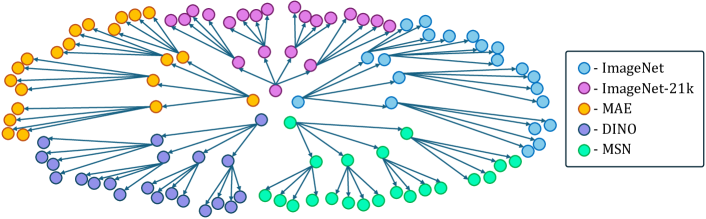
Figure 6: ViT Tree Heritage Recovery (VTHR) Dataset Overview: Our dataset contains $3$ Model Graph splits. Each Model Graph contains $105$ nodes across five Model Trees rooted at different pre-trained ViT models found on Hugging Face. Each node represents a model that was fine-tuned on different datasets with different configurations. We visualize the structure of a single Model Graphpage

6.1 ViT Tree Heritage Recovery (VTHR) dataset results

Full fine-tuning.

We start with a simplified setting of recovering the Model Trees independently (i.e., a Model Graph with a single Model Tree). We set $L$ from $\cref{eq:mother_{d}istance_{f}ull_{f}t}$ to be all the dense layers of the model. For $3$ out of the $5$ Model Trees in the dataset, MoTHer successfully reconstructs the tree structure with perfect accuracy. The other two Model Trees suffered from a wrong directional score, which resulted in an imperfect reconstruction, we show the full breakdown in tab:model_tree_results. Next, we test our method on the entire Model Graph. This requires first clustering the set of nodes, as seen in tab:model_tree_results, MoTHer recovered the Model Graph with an accuracy of $0.89$. Notably, the clustering succeeded with perfect accuracy, resulting in a similar result as the independent Model Trees, in sec:ablations show the relation between the size of the Model Graph and the accuracy of the clustering.

LoRA fine-tuning.

We proceed by testing MoTHer on the LoRA dataset splits, similar to the previous section, we first perform MoTHer recovery on the Model Trees independently. We set $L$ from $\cref{eq:mother_{d}istance_{l}ora}$ to be all the LoRA fine-tuned value layers of the model (by default, LoRA does not train the dense layers). As can be seen in tab:model_tree_results, when the different models have varying LoRA ranks, we successfully reconstruct all Model Trees with perfect accuracy. In contrast, when all models use the same rank, the variance between different models decreases, resulting in a slightly reduced accuracy for one of the $5$ Model Trees. When working with the entire Model Graph, the difference in the LoRA matrix between models from different Model Trees is (almost) guaranteed to be full rank. As before, the clustering succeeded with perfect accuracy, see tab:model_tree_results for the Model Graph results.

To ablate whether the LoRA-based $\ell_{LoRA}$ distance defined in eq:mother_distance_lora is necessary, we repeat the above experiment with $\ell_{FT}$. Not using the low-rank distance prior reduces the results on LoRA-V by $22\%$ from perfect accuracy to $0.78$, demonstrating the significance of $\ell_{LoRA}$ for LoRA fine-tuned models.

Table 1: MoTHer Results on VTHR: MoTHer Recovery achieves high accuracy both for individual Model Trees and entire Model Graphs across all VTHR splits

VTHR Split	Model Tree Root					Model Graph
	ImageNet	ImageNet-21k	MAE	DINO	MSN
FT	1.0	1.0	0.95	0.5	1.0	0.89
LoRA-F	1.0	1.0	1.0	1.0	0.8	0.96
LoRA-V	1.0	1.0	1.0	1.0	1.0	1.0

page

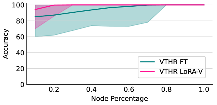
Figure 7: Clustering Robustness to Small Model Graphs: In both cases, the clustering works with high accuracy even for small Model Graphspage

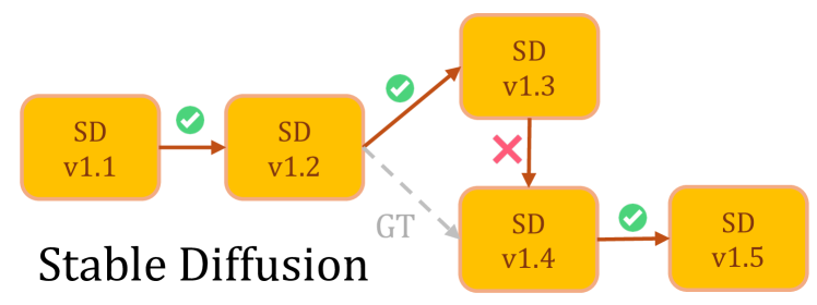
Figure 8: Stable Diffusion Model Tree: We successfully reconstruct all but a single edge, where the estimated weight distance was incorrect but the direction was correctpage

6.2 In-the-wild MoTHer recovery

Having shown we can reconstruct the Model Graph structure with high accuracy on the VTHR dataset, we now attempt to reconstruct the Model Tree of in-the-wild models found on Hugging Face. We note that the examples below are unique in that they provide a relatively detailed description of their model hierarchy. We are not aware of other model families that provide such a detailed description, this provides a unique opportunity for us to test our method in a real-world situation with ground truth metrics but also emphasizes the relevance of the MoTHer recovery task.

Llama 2.

The Llama papers (33; 30) describe in detail the training hierarchy of their models and even include a figure that shows the model hierarchy. As such, we can evaluate MoTHer on the Llama family compare to the ground truth they provide. We use the official Llama 2 models provided by Meta, which contain $5$ models in $3$ levels of hierarchy. We use the $\ell_{FT}$ distance described above, since the fine-tuned models are specialized versions of the foundation model, we label each model as a specialization trained model. Our method successfully reconstructs the correct structure of the Model Tree with perfect accuracy, we plot the full Model Tree in fig:llama_tree.

Stable Diffusion

The Hugging Face model cards for Stable Diffusion describe a $4$ level hierarchy spanning $5$ of their models. We use the $\ell_{FT}$ distance described above, however, since the different model versions are better and more generalized foundation models we treat them as generalization nodes. As seen in fig:sd_tree, MoTHer successfully reconstructs all but a single edge, incorrectly placing “Stable Diffusion 1.4” as a descendent of “Stable Diffusion 1.3”, instead of a sibling. Notably, the mistake occurred due to a wrong distance, as the directional score returned the correct edge direction.

6.3 Ablations

page

Robustness to similar models.

Foundation models often come with fine-tuning “recipes”, as such, many publicly available models are almost identical to each other, often with just a different seed. We therefore test the robustness of MoTHer with $3$ identically fine-tuned versions of ViT that used different seeds. In all $3$ cases, the distance between sibling models was greater than to the parent model, allowing us to correctly recover the Model Tree.

Robustness to smaller Model Trees.

We ablate whether MoTHer is sensitive to the size of the Model Tree. We therefore sample sub Model Trees of varying size. For each of the $5$ Model Trees, each experiment was repeated $10$ times, with a newly sampled random sub Model Tree each time ($50$ sub Model Trees for each tested size). Indeed, the number of nodes in a Model Tree size did not impact the results (see tab:small_trees). We note that we did not test MoTHer on huge, web scale Model Graphs, in sec:discussion we discuss scaling MoTHer recovery to web scale Model Graphs.

Clustering robustness to smaller Model Graphs

We now test whether the clustering succeeds for small Model Graphs. As seen in fig:clustering_robustness, even with as little as $10$ models (across $5$ Model Trees), the clustering achieves high accuracy, indicating MoTHer recovery could be performed even for small, yet diverse Model Graphs.

Other directional scores.

Our directional score (eq:kurtosis) uses kurtosis to estimate the distributional change in outliers of weight values. However, other directional scores may be favorable. We compared the performance using the mean, variance, skewness, kurtosis, and entropy. To do so, we fine-tuned each of the root models from the VTHR dataset and extracted intermediate weights throughout the training process. The kurtosis is the only metric that demonstrated consistent monotonicity across the different models (see app:other_directional_scores).

Effect of layers types.

Neural networks often contain multiple layer types (e.g., linear, convolutional, attention). We therefore study the change in the directional score for different layer types throughout the fine-tuning process. Despite different types of layers exhibiting similar trends on average, the dense layer remained consistent across all Model Trees (see app:layer_types).

7 Discussion and Limitations

page

Training stage supervision.

Throughout the paper we assumed the training stage is known in advance. While for many use cases this is a reasonable assumption, finding a method to automatically infer the stage based on the model weights would allow for greater applicability in cases where the training stage supervision is missing. Alternatively, one could extend MoTHer with methods for identifying the direction of an edge that do not rely on the training stage.

MoTHer Recovery at web scale.

This paper makes the first step in recovering the Model Graph of trained neural networks. However, recovering web scale Model Graphs requires significant computational resources for storing the hundreds of thousands of models and computing their distance matrices. Additionally, as Model Trees continually grow and new Model Trees are added to the Model Graph, manually documenting these changes is infeasible. New algorithms are likely needed for efficient weight distance computation and for continuously updating the Model Graph with new models and Model Trees. Projecting the model weights to some lower dimensional embedding space could decrease the computational costs and be more suitable for web scale Model Graphs.

Inferring graph properties from model metadata.

MoTHer recovery is the first step towards indexing the AI model universe. Akin to digital maps of the world, once a Model Graph has been constructed, additional layers that contain node metadata (e.g., training dataset, training hyper-parameters, model affiliation) could be added to it. Given partial data on a limited number of nodes, it may be possible to train a Graph Neural Network (GNN) (16) or similar methods (3; 22; 37) on the Model Graph to estimate the attributes of other nodes.

8 Conclusion

page Although model weights fully characterize a model’s capabilities, their lack of interpretability has left them under-explored. However, with the growing number of publicly available models, including over 600,000 models on Hugging Face, model weights are set to become a significant data modality. We propose the Model Graph, a data structure for describing the hereditary relations between models. To recover the structure of a Model Graph, we introduce the task of MoTHer Recovery, which aims to map out unknown Model Graphs. We identify two key properties of model weights that enable the recovery of Model Graphs. We validate our approach by successfully reconstructing the Model Graph of in-the-wild production models. Taken together, the Model Graph and MoTHer Recovery make an exciting first step toward understanding the origin of models.

Appendix A Dataset Details

page For all VTHR splits, we use the following models as the Model Tree roots taken from Hugging Face:

• https://huggingface.co/google/vit-base-patch16-224

• https://huggingface.co/google/vit-base-patch16-224-in21k

• https://huggingface.co/facebook/vit-mae-base

• https://huggingface.co/facebook/dino-vitb16

• https://huggingface.co/facebook/vit-msn-base

For the FT split, to prevent model overfitting, we use larger datasets of 10K samples rather than the original 1K used in the VTAB benchmark. Each model uses a different randomly sampled seed. See table:full_ft_hyperparams for additional hyper-parameters.

Apart from the rank and seeds, both LoRA-F and LoRA-V use the same hyper-parameters. LoRA-F uses a fixed rank and alpha of $16$, LoRA-V uses ranks sampled randomly out of the options shown in table:lora_v_hyperparams. Both use the VTAB-1K datasets shown in table:lora_v_hyperparams and random seeds. See table:full_ft_hyperparams for additional hyper-parameters.

Table 2: Full Fine-tuning Hyper-parameters

Name	Value
lr	$2e-4$
batch_size	$64$
epochs	$5$
datasets	cifar100, svhn, patch_camelyon, clevr-count, clevr-distance, dmlab

page

Table 3: LoRA Varying Ranks Fine-tuning Hyper-parameters

Name	Value
lora_rank ($r$)	$8,16,32,64$
lora_alpha ($\alpha$)	$8,16,32,64$
lr	$9e-3$
batch_size	$128$
epochs	$20$
datasets	cifar100, caltech101, dtd, flower102, pet37, svhn, patch_camelyon, clevr-count, clevr-distance, dmlab, kitti, dsprites-location, dsprites-orientation, smallnorb-azimuth, smallnorb-elevation

page

Appendix B Llama2 and Stable Diffusion Models

For the Llama2 models we used the following versions found on Hugging Face:

• https://huggingface.co/meta-llama/Llama-2-7b-hf

• https://huggingface.co/meta-llama/CodeLlama-7b-hf

• https://huggingface.co/meta-llama/CodeLlama-7b-Instruct-hf

• https://huggingface.co/meta-llama/CodeLlama-7b-Python-hf

• https://huggingface.co/meta-llama/Llama-2-7b-chat-hf

For Stable Diffusion we used the following versions found on Hugging Face:

• https://huggingface.co/CompVis/stable-diffusion-v1-1

• https://huggingface.co/CompVis/stable-diffusion-v1-2

• https://huggingface.co/CompVis/stable-diffusion-v1-3

• https://huggingface.co/CompVis/stable-diffusion-v1-4

• https://huggingface.co/runwayml/stable-diffusion-v1-5

Table 4: Robustness to smaller Model Trees: Accuracy over VTHR sub Model Trees, mostly unaffected by tree size

% Model (# Models)	20% (4)	40% (8)	60% (13)	80% (17)	100% (21)
Accuracy	0.87 $\pm 0.25$	0.9 $\pm 0.18$	0.88 $\pm 0.20$	0.89 $\pm 0.19$	0.89

page

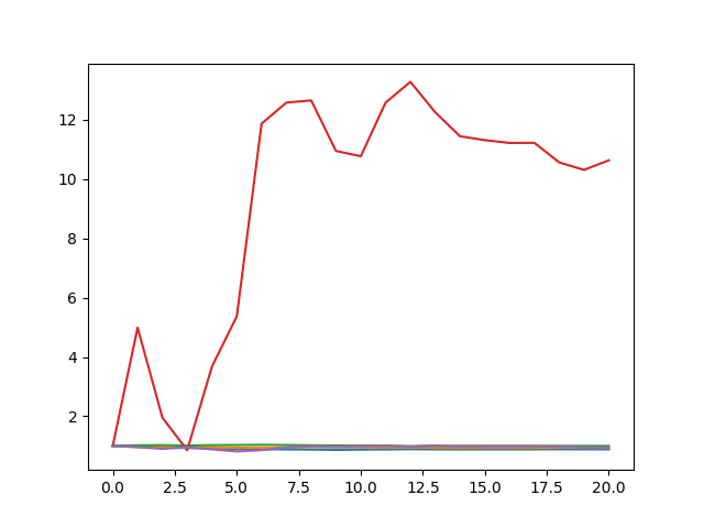
Figure 9: Mean

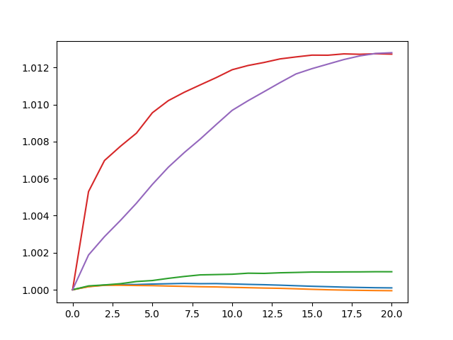
Figure 10: Variance

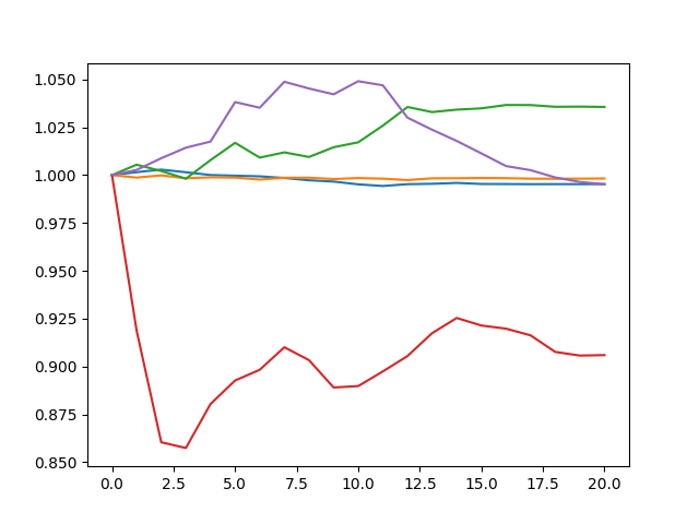
Figure 11: Skewness

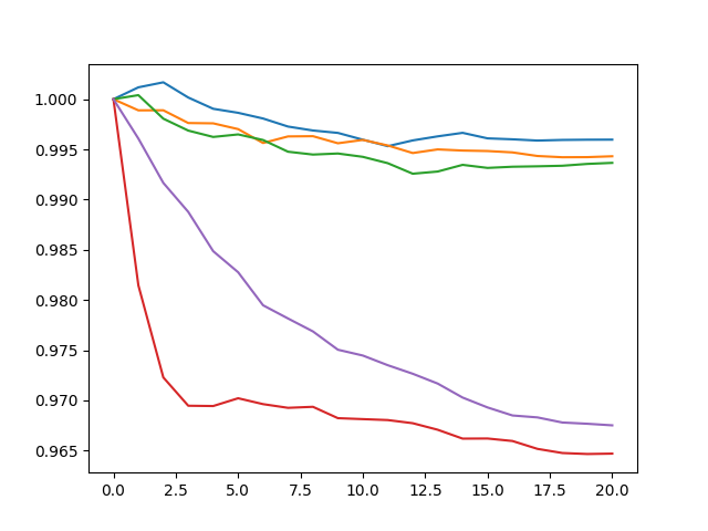
Figure 12: Kurtosis

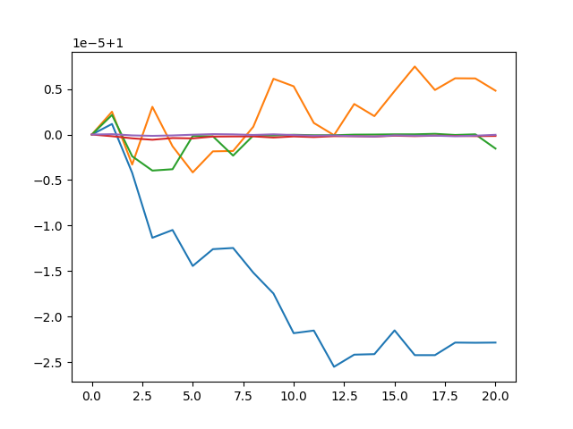
Figure 13: Entropy

Figure 14: Other directional scores: We compute the different types of directional scores throughout the fine-tuning process.the kurtosis is the only metric that remained consistently (almost) monotonic. Each color represents a different Model Tree rootpage

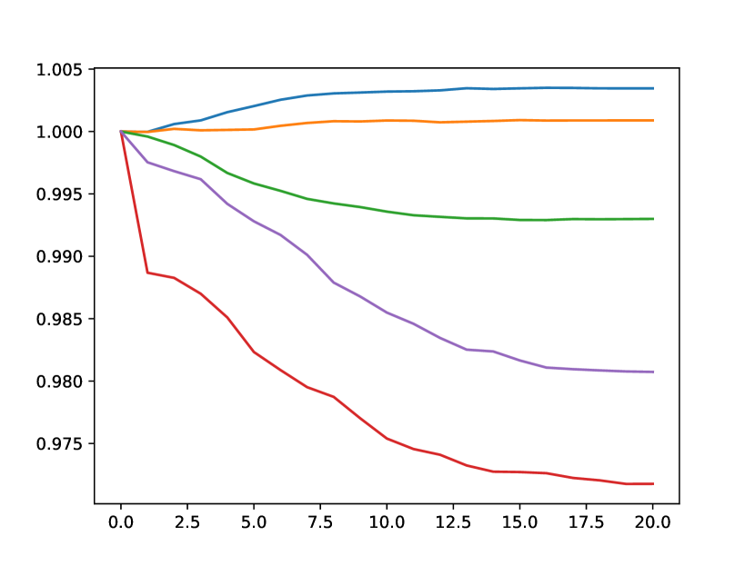
Figure 15: Query

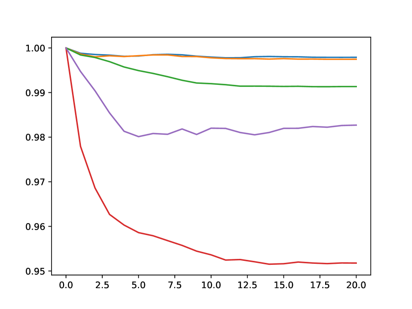
Figure 16: Value

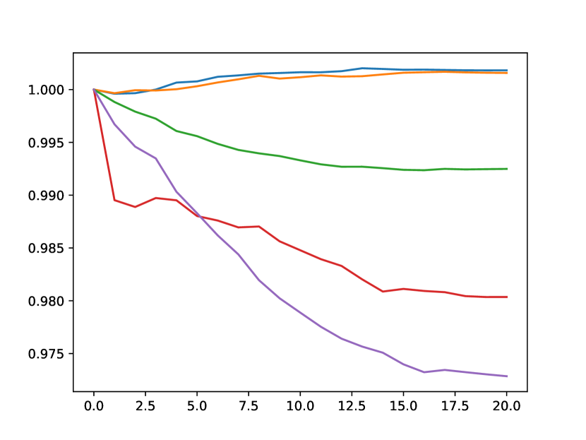
Figure 17: Key

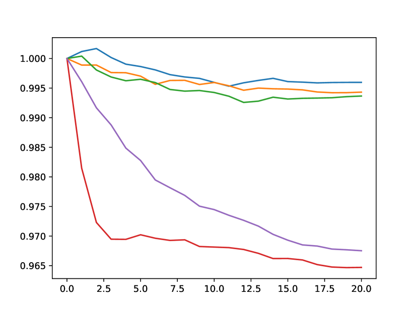
Figure 18: Dense

Figure 19: Effect of Layer Type: We compute the directional score throughout the fine-tuning process. The Dense layer is the only layer that remained consistently (almost) monotonic. Each color represents a different Model Tree root page

References

- Antognini and Sohl-Dickstein (2018) Joseph Antognini and Jascha Sohl-Dickstein. Pca of high dimensional random walks with comparison to neural network training. Advances in Neural Information Processing Systems, 31, 2018.
- Brin and Page (1998) Sergey Brin and Lawrence Page. The anatomy of a large-scale hypertextual web search engine. Computer networks and ISDN systems, 30(1-7):107–117, 1998.
- Bruna et al. (2013) Joan Bruna, Wojciech Zaremba, Arthur Szlam, and Yann LeCun. Spectral networks and locally connected networks on graphs. arXiv preprint arXiv:1312.6203, 2013.
- Chefer et al. (2021) Hila Chefer, Shir Gur, and Lior Wolf. Transformer interpretability beyond attention visualization. In Proceedings of the IEEE/CVF conference on computer vision and pattern recognition, pages 782–791, 2021.
- Chu (1965) Yoeng-Jin Chu. On the shortest arborescence of a directed graph. Scientia Sinica, 14:1396–1400, 1965.
- Dar et al. (2022) Guy Dar, Mor Geva, Ankit Gupta, and Jonathan Berant. Analyzing transformers in embedding space. arXiv preprint arXiv:2209.02535, 2022.
- Darwin et al. (2009) Charles Darwin, John Wyon Burrow, and John Wyon Burrow. The origin of species by means of natural selection: or, the preservation of favored races in the struggle for life. AL Burt New York, 2009.
- Dosovitskiy et al. (2020) Alexey Dosovitskiy, Lucas Beyer, Alexander Kolesnikov, Dirk Weissenborn, Xiaohua Zhai, Thomas Unterthiner, Mostafa Dehghani, Matthias Minderer, Georg Heigold, Sylvain Gelly, et al. An image is worth 16x16 words: Transformers for image recognition at scale. arXiv preprint arXiv:2010.11929, 2020.
- Dravid et al. (2023) Amil Dravid, Yossi Gandelsman, Alexei A Efros, and Assaf Shocher. Rosetta neurons: Mining the common units in a model zoo. In Proceedings of the IEEE/CVF International Conference on Computer Vision, pages 1934–1943, 2023.
- Edmonds et al. (1967) Jack Edmonds et al. Optimum branchings. Journal of Research of the national Bureau of Standards B, 71(4):233–240, 1967.
- Eilertsen et al. (2020) Gabriel Eilertsen, Daniel Jönsson, Timo Ropinski, Jonas Unger, and Anders Ynnerman. Classifying the classifier: dissecting the weight space of neural networks. arXiv preprint arXiv:2002.05688, 2020.
- Erkoç et al. (2023) Ziya Erkoç, Fangchang Ma, Qi Shan, Matthias Nießner, and Angela Dai. Hyperdiffusion: Generating implicit neural fields with weight-space diffusion. In Proceedings of the IEEE/CVF International Conference on Computer Vision, pages 14300–14310, 2023.
- Gabow et al. (1986) Harold N Gabow, Zvi Galil, Thomas Spencer, and Robert E Tarjan. Efficient algorithms for finding minimum spanning trees in undirected and directed graphs. Combinatorica, 6(2):109–122, 1986.
- Gallagher and Downs (1997a) Marcus Gallagher and Tom Downs. Visualization of learning in neural networks using principal component analysis. In Proc of Int Conf on Computational Intelligence and Multimedia Applications, edited by: Varma, B. and Yao, X., Australia, pages 327–331. Citeseer, 1997a.
- Gallagher and Downs (1997b) Marcus Gallagher and Tom Downs. Weight space learning trajectory visualization. In Proc. Eighth Australian Conference on Neural Networks, Melbourne, pages 55–59. Citeseer, 1997b.
- Hamilton et al. (2017) Will Hamilton, Zhitao Ying, and Jure Leskovec. Inductive representation learning on large graphs. Advances in neural information processing systems, 30, 2017.
- He et al. (2015) Kaiming He, Xiangyu Zhang, Shaoqing Ren, and Jian Sun. Delving deep into rectifiers: Surpassing human-level performance on imagenet classification. In Proceedings of the IEEE international conference on computer vision, pages 1026–1034, 2015.
- He et al. (2016) Kaiming He, Xiangyu Zhang, Shaoqing Ren, and Jian Sun. Deep residual learning for image recognition. In Proceedings of the IEEE conference on computer vision and pattern recognition, pages 770–778, 2016.
- Horwitz et al. (2024) Eliahu Horwitz, Jonathan Kahana, and Yedid Hoshen. Recovering the pre-fine-tuning weights of generative models. arXiv preprint arXiv:2402.10208, 2024.
- Hu et al. (2021) Edward J Hu, Yelong Shen, Phillip Wallis, Zeyuan Allen-Zhu, Yuanzhi Li, Shean Wang, Lu Wang, and Weizhu Chen. Lora: Low-rank adaptation of large language models. arXiv preprint arXiv:2106.09685, 2021.
- Katz et al. (2024) Shahar Katz, Yonatan Belinkov, Mor Geva, and Lior Wolf. Backward lens: Projecting language model gradients into the vocabulary space. arXiv preprint arXiv:2402.12865, 2024.
- Kipf and Welling (2016) Thomas N Kipf and Max Welling. Semi-supervised classification with graph convolutional networks. arXiv preprint arXiv:1609.02907, 2016.
- Kofinas et al. (2024) Miltiadis Kofinas, Boris Knyazev, Yan Zhang, Yunlu Chen, Gertjan J Burghouts, Efstratios Gavves, Cees GM Snoek, and David W Zhang. Graph neural networks for learning equivariant representations of neural networks. arXiv preprint arXiv:2403.12143, 2024.
- Kong et al. (2016) Tao Kong, Anbang Yao, Yurong Chen, and Fuchun Sun. Hypernet: Towards accurate region proposal generation and joint object detection. In Proceedings of the IEEE conference on computer vision and pattern recognition, pages 845–853, 2016.
- Lim et al. (2023) Derek Lim, Haggai Maron, Marc T Law, Jonathan Lorraine, and James Lucas. Graph metanetworks for processing diverse neural architectures. arXiv preprint arXiv:2312.04501, 2023.
- Navon et al. (2023a) Aviv Navon, Aviv Shamsian, Idan Achituve, Ethan Fetaya, Gal Chechik, and Haggai Maron. Equivariant architectures for learning in deep weight spaces. In International Conference on Machine Learning, pages 25790–25816. PMLR, 2023a.
- Navon et al. (2023b) Aviv Navon, Aviv Shamsian, Ethan Fetaya, Gal Chechik, Nadav Dym, and Haggai Maron. Equivariant deep weight space alignment. arXiv preprint arXiv:2310.13397, 2023b.
- Peebles et al. (2022) William Peebles, Ilija Radosavovic, Tim Brooks, Alexei A Efros, and Jitendra Malik. Learning to learn with generative models of neural network checkpoints. arXiv preprint arXiv:2209.12892, 2022.
- Rombach et al. (2022) Robin Rombach, Andreas Blattmann, Dominik Lorenz, Patrick Esser, and Björn Ommer. High-resolution image synthesis with latent diffusion models. In Proceedings of the IEEE/CVF conference on computer vision and pattern recognition, pages 10684–10695, 2022.
- Roziere et al. (2023) Baptiste Roziere, Jonas Gehring, Fabian Gloeckle, Sten Sootla, Itai Gat, Xiaoqing Ellen Tan, Yossi Adi, Jingyu Liu, Tal Remez, Jérémy Rapin, et al. Code llama: Open foundation models for code. arXiv preprint arXiv:2308.12950, 2023.
- Selvaraju et al. (2017) Ramprasaath R Selvaraju, Michael Cogswell, Abhishek Das, Ramakrishna Vedantam, Devi Parikh, and Dhruv Batra. Grad-cam: Visual explanations from deep networks via gradient-based localization. In Proceedings of the IEEE international conference on computer vision, pages 618–626, 2017.
- Shokri et al. (2017) Reza Shokri, Marco Stronati, Congzheng Song, and Vitaly Shmatikov. Membership inference attacks against machine learning models. In 2017 IEEE symposium on security and privacy (SP), pages 3–18. IEEE, 2017.
- Touvron et al. (2023) Hugo Touvron, Louis Martin, Kevin Stone, Peter Albert, Amjad Almahairi, Yasmine Babaei, Nikolay Bashlykov, Soumya Batra, Prajjwal Bhargava, Shruti Bhosale, et al. Llama 2: Open foundation and fine-tuned chat models. arXiv preprint arXiv:2307.09288, 2023.
- Unterthiner et al. (2020) Thomas Unterthiner, Daniel Keysers, Sylvain Gelly, Olivier Bousquet, and Ilya Tolstikhin. Predicting neural network accuracy from weights. arXiv preprint arXiv:2002.11448, 2020.
- Virtanen et al. (2020) Pauli Virtanen, Ralf Gommers, Travis E. Oliphant, Matt Haberland, Tyler Reddy, David Cournapeau, Evgeni Burovski, Pearu Peterson, Warren Weckesser, Jonathan Bright, Stéfan J. van der Walt, Matthew Brett, Joshua Wilson, K. Jarrod Millman, Nikolay Mayorov, Andrew R. J. Nelson, Eric Jones, Robert Kern, Eric Larson, C J Carey, İlhan Polat, Yu Feng, Eric W. Moore, Jake VanderPlas, Denis Laxalde, Josef Perktold, Robert Cimrman, Ian Henriksen, E. A. Quintero, Charles R. Harris, Anne M. Archibald, Antônio H. Ribeiro, Fabian Pedregosa, Paul van Mulbregt, and SciPy 1.0 Contributors. SciPy 1.0: Fundamental Algorithms for Scientific Computing in Python. Nature Methods, 17:261–272, 2020.
- Wang et al. (2024) Kai Wang, Zhaopan Xu, Yukun Zhou, Zelin Zang, Trevor Darrell, Zhuang Liu, and Yang You. Neural network diffusion. arXiv preprint arXiv:2402.13144, 2024.
- Winter et al. (2024) Daniel Winter, Niv Cohen, and Yedid Hoshen. Classifying nodes in graphs without gnns. arXiv preprint arXiv:2402.05934, 2024.
- Zhai et al. (2019) Xiaohua Zhai, Joan Puigcerver, Alexander Kolesnikov, Pierre Ruyssen, Carlos Riquelme, Mario Lucic, Josip Djolonga, Andre Susano Pinto, Maxim Neumann, Alexey Dosovitskiy, et al. A large-scale study of representation learning with the visual task adaptation benchmark. arXiv preprint arXiv:1910.04867, 2019.
- Zhang et al. (2024) Baoquan Zhang, Chuyao Luo, Demin Yu, Xutao Li, Huiwei Lin, Yunming Ye, and Bowen Zhang. Metadiff: Meta-learning with conditional diffusion for few-shot learning. In Proceedings of the AAAI Conference on Artificial Intelligence, pages 16687–16695, 2024.
- Zhou et al. (2024) Allan Zhou, Kaien Yang, Kaylee Burns, Adriano Cardace, Yiding Jiang, Samuel Sokota, J Zico Kolter, and Chelsea Finn. Permutation equivariant neural functionals. Advances in Neural Information Processing Systems, 36, 2024.
- Zhou et al. (2016) Bolei Zhou, Aditya Khosla, Agata Lapedriza, Aude Oliva, and Antonio Torralba. Learning deep features for discriminative localization. In Proceedings of the IEEE conference on computer vision and pattern recognition, pages 2921–2929, 2016.