Phased Consistency Model

Fu-Yun Wang1  Zhaoyang Huang2  Alexander William Bergman3,6 Dazhong Shen4
Peng Gao4  Michael Lingelbach3,6  Keqiang Sun1  Weikang Bian1
Guanglu Song5  Yu Liu4  Hongsheng Li1 Xiaogang Wang1
1Multimedia Laboratory, The Chinese University of Hong Kong 2Avolution AI
3Hedra 4Shanghai AI Laboratory 5Sensetime Research 6Stanford University
{fywang@link, hsli@ee, xgwang@ee}.cuhk.edu.hk
Abstract

The consistency model (CM) has recently made significant progress in accelerating the generation of diffusion models. However, its application to high-resolution, text-conditioned image generation in the latent space (a.k.a., LCM) remains unsatisfactory. In this paper, we identify three key flaws in the current design of LCM. We investigate the reasons behind these limitations and propose the Phased Consistency Model (PCM), which generalizes the design space and addresses all identified limitations. Our evaluations demonstrate that PCM significantly outperforms LCM across 1–16 step generation settings. While PCM is specifically designed for multi-step refinement, it achieves even superior or comparable 1-step generation results to previously state-of-the-art specifically designed 1-step methods. Furthermore, we show that PCM’s methodology is versatile and applicable to video generation, enabling us to train the state-of-the-art few-step text-to-video generator. More details available at https://g-u-n.github.io/projects/pcm/.

[Uncaptioned image]

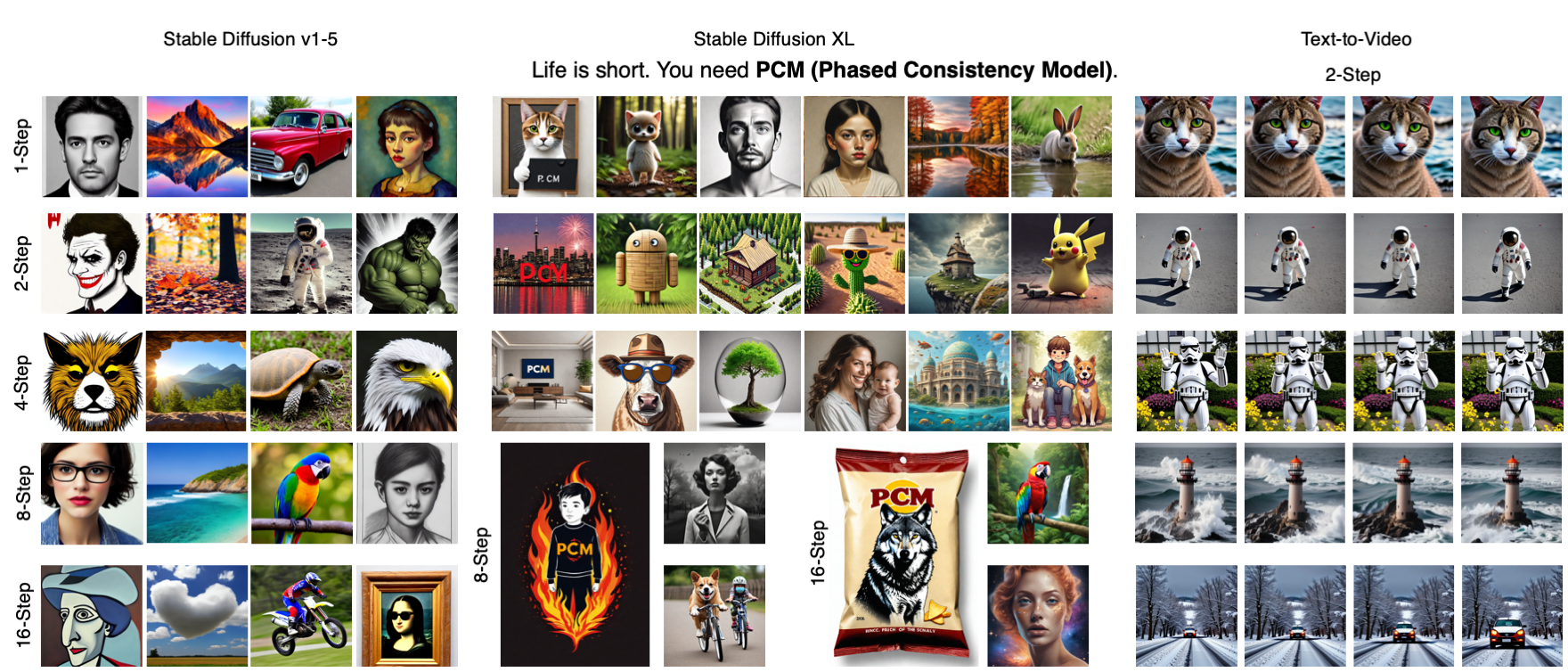
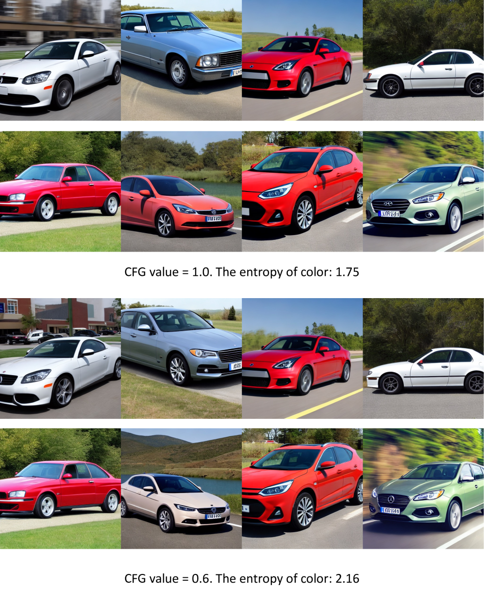
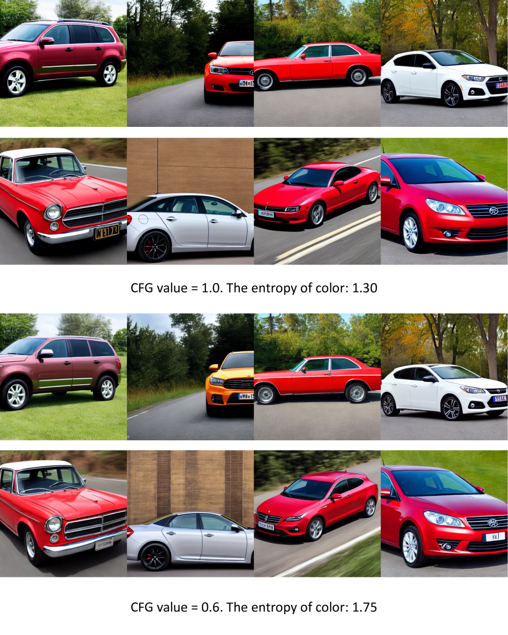
Figure 1: Summative motivation. We observe and summarize three crucial limitations for (latent) consistency models, and generalize the design space, well tackling all these limitations.

1 Introduction

Refer to caption


Figure 2: Phased Consistency Model: Towards stable and fast image and video generation.

Diffusion models [11, 9, 36, 41] have emerged as the dominant methodology for generative image synthesis [27, 24, 5]. These models have shown the ability to generate high-quality and diverse examples conditioned on varying signals. At their core, diffusion models rely on an iterative evaluation to generate new samples. This iterative evaluation trajectory models the probability flow ODE (PF-ODE) [35, 36] that transforms an initial normal distribution to a target real data distribution. However, the iterative nature of these models makes the generation of new samples time-intensive and resource-consuming. To address this challenge, consistency models [35, 34] have emerged to reduce the number of iterative steps required to generate a sample. These models work by training a model that enforces the self-consistency [35] property: any point along a trajectory shall be mapped to the same solution. These models have been extended to high-resolution text-to-image synthesis with latent diffusion models (LCM) [21]. Despite the improvements in efficiency and the ability to generate results in a few steps, the quality of such models for text-to-image synthesis is still limited.

We show that the current design of LCMs is flawed, causing inevitable drawbacks in consistency, controllability, and efficiency during image sampling. Fig. 1 illustrates our observations of LCM. The limitations are listed as follows:

  1. (1)

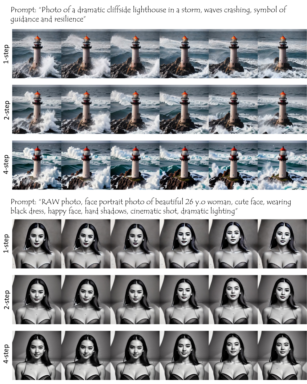
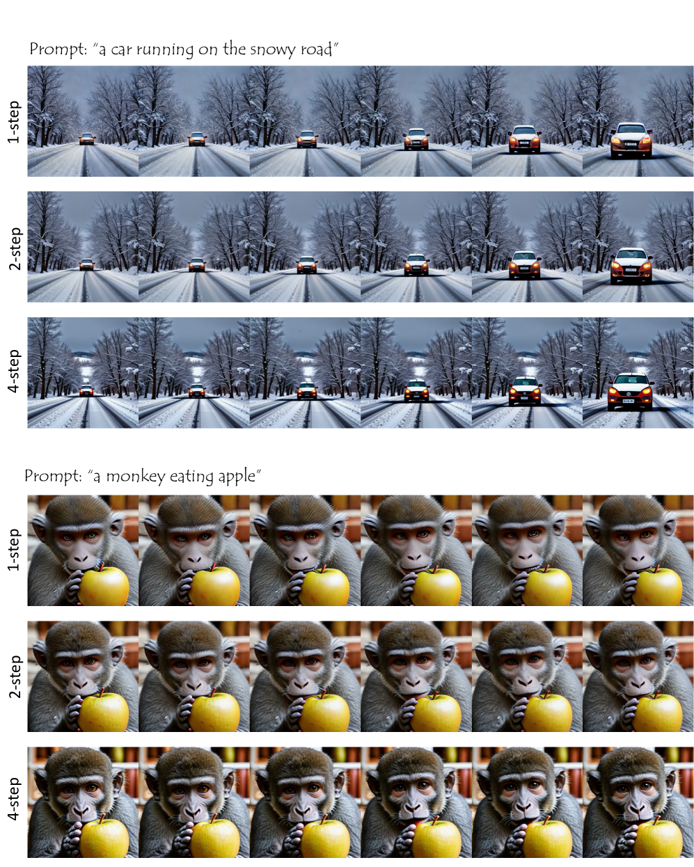
    Consistency. Due to the specific consistency property, CMs and LCMs can only use the purely stochastic multi-step sampling algorithm, which assumes that the accumulated noise variable in each generative step is independent and causes varying degrees of stochasticity for different inference-step settings. As a result, we can find inconsistency among the results generated with the same seeds in different inference steps. LCM (and many other types of fast-generation methods) typically fail to stably generate satisfactory results in both few and many inference steps.

  2. (2)

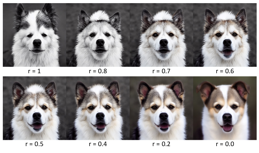
    Controllability. Even though Stable Diffusion can accept classifier-free guidance (CFG) [10] in a wide range of inference steps (i.e. 2-15), equipped with LCM weights, they can only accept CFG with 1-2 steps. Larger values of CFG would cause the exposure problem. This brings more difficulty for the hyper-parameter selection. Additionally, we find that the LCM is insensitive to the negative prompt. As shown in the figure, it still generates black dogs even when the negative prompt is set to “black dog". Both the phenomenons reduce the controllability on image generation. We show the deep reasons behind this are the CFG-augmented ODE solver applied in the consistency distillation stage.

  3. (3)

    Efficiency. We find that LCM tends to generate much inferior results at the few-step settings, especially in less than 4 inference steps, which limits the sampling efficiency. We argue that the reason lies in the traditional L2 loss or the Huber loss used in the LCM procedure, which is insufficient for the fine-grain supervision in low-step settings.

Our proposed model, PCM, can tackle the discussed limitations of LCM and is easy to train. Specifically, instead of mapping all points along the ODE trajectory to the same solution, PCM phases the ODE trajectory into several sub-trajectories and only enforces the self-consistency property on each sub-trajectory. Therefore, PCM can sample results along the solution points of different sub-trajectories in a deterministic manner without error accumulation.

As an example shown in Figure 2, we train PCM with two sub-trajectories, with 3 edge points including 𝐱Tsubscript𝐱𝑇\mathbf{x}_{T}, 𝐱0subscript𝐱0\mathbf{x}_{0}, and 𝐱T/2subscript𝐱𝑇2\mathbf{x}_{\lfloor T/2\rfloor} selected. Thereby, we can achieve 2-step deterministic sampling (i.e., 𝐱T𝐱T/2𝐱0subscript𝐱𝑇subscript𝐱𝑇2subscript𝐱0\mathbf{x}_{T}\rightarrow\mathbf{x}_{\lfloor T/2\rfloor}\rightarrow\mathbf{x}_{0} ) for generation. In this way, PCM avoids the stochasticity error accumulation for sampling.

The phased nature of PCM leads to another advantage. For distillation, we can choose to use a normal ODE solver without the CFG strategy alternatively in the consistency distillation stage, which is not viable in LCMs. As a result, PCM can optionally use larger CFG for inference and be more responsive to the negative prompt. Additionally, to improve the sample quality for few-step setting, we propose an adversarial loss in the latent space for more fine-grained supervision.

In summary, we dive into the design of (latent) consistency models, analyze the reasons for their unsatisfactory generation characteristics, and propose effective strategies for tackling these limitations. We validate the effectiveness of PCM on widely recognized image generation benchmarks with stable diffusion v1-5 (0.9 B) [27] and stable diffusion XL (3B) [24] and video generation benchmarks with AnimateLCM [39]. Vast experimental results show the advancements of PCM.

2 Preliminaries

Refer to caption
Figure 3: (Left) Illustrative comparison of diffusion models [9], consistency models [35], consistency trajectory models [12], and our phased consistency model. (Right) Simplified visualization of the forward SDE and reverse-time PF-ODE trajectories.

Diffusion models define a forward conditional probability path, with a general representation of αt𝐱0+σtϵsubscript𝛼𝑡subscript𝐱0subscript𝜎𝑡bold-italic-ϵ\alpha_{t}\mathbf{x}_{0}+\sigma_{t}\bm{\epsilon} for intermediate distribution t(𝐱|𝐱0)subscript𝑡conditional𝐱subscript𝐱0\mathbb{P}_{t}(\mathbf{x}|\mathbf{x}_{0}) conditioned on 𝐱00similar-tosubscript𝐱0subscript0\mathbf{x}_{0}\sim\mathbb{P}_{0}, which is equivalent to the stochasitic differential equation d𝐱t=ft𝐱tdt+gtd𝒘tdsubscript𝐱𝑡subscript𝑓𝑡subscript𝐱𝑡d𝑡subscript𝑔𝑡dsubscript𝒘𝑡\mathrm{d}\mathbf{x}_{t}=f_{t}\mathbf{x}_{t}\mathrm{d}t+g_{t}\mathrm{d}\bm{w}_{t} with 𝒘tsubscript𝒘𝑡\bm{w}_{t} denoting the standard Winer process, ft=dlogαtdtsubscript𝑓𝑡dsubscript𝛼𝑡subscriptd𝑡f_{t}=\frac{\mathrm{d}\log\alpha_{t}}{\mathrm{d}_{t}} and gt2=dσt2dt2dlogαtdtσt2superscriptsubscript𝑔𝑡2dsuperscriptsubscript𝜎𝑡2d𝑡2dsubscript𝛼𝑡d𝑡superscriptsubscript𝜎𝑡2g_{t}^{2}=\frac{\mathrm{d}\sigma_{t}^{2}}{\mathrm{d}t}-2\frac{\mathrm{d}\log\alpha_{t}}{\mathrm{d}t}\sigma_{t}^{2}. There exists infinite reverse time equivalent flow that the solution trajectory still follows marginal distribution t(𝐱)subscript𝑡𝐱\mathbb{P}_{t}(\mathbf{x}), having a general SDE formula, i.e., d𝐱=[ftgt2𝐱logt(𝐱)]dt+gtd𝒘d𝐱delimited-[]subscript𝑓𝑡superscriptsubscript𝑔𝑡2subscript𝐱subscript𝑡𝐱d𝑡subscript𝑔𝑡d𝒘\mathrm{d}\mathbf{x}=\left[f_{t}-g_{t}^{2}\nabla_{\mathbf{x}}\log\mathbb{P}_{t}(\mathbf{x})\right]\mathrm{d}t+g_{t}\mathrm{d}\bm{w}. Among all the reverse time flows, there exists a deterministic flow for transition, which is represented by the ODE d𝐱=[ftgt2/2𝐱logt(𝐱)]dtd𝐱delimited-[]subscript𝑓𝑡subscriptsuperscript𝑔2𝑡2subscript𝐱subscript𝑡𝐱d𝑡\displaystyle\smash{\mathrm{d}\mathbf{x}=\left[f_{t}-g^{2}_{t}/2\nabla_{\mathbf{x}}\log\mathbb{P}_{t}(\mathbf{x})\right]\mathrm{d}t}. For training of diffusions, a neural network is typically learned to estimate the score of marginal distribution t(𝐱t)subscript𝑡subscript𝐱𝑡\mathbb{P}_{t}(\mathbf{x}_{t}), which is equivalent to 𝒔ϕ(𝐱,t)𝐱logt(𝐱)=𝔼𝐱0(𝐱0|𝐱)[𝐱logt(𝐱|𝐱0)]subscript𝒔bold-italic-ϕ𝐱𝑡subscript𝐱subscript𝑡𝐱subscript𝔼similar-tosubscript𝐱0conditionalsubscript𝐱0𝐱delimited-[]subscript𝐱subscript𝑡conditional𝐱subscript𝐱0\bm{s}_{\bm{\phi}}(\mathbf{x},t)\approx\nabla_{\mathbf{x}}\log\mathbb{P}_{t}(\mathbf{x})=\mathbb{E}_{\mathbf{x}_{0}\sim\mathbb{P}(\mathbf{x}_{0}|\mathbf{x})}\left[\nabla_{\mathbf{x}}\log\mathbb{P}_{t}(\mathbf{x}|\mathbf{x}_{0})\right]. Substitue the 𝐱logt(x)subscript𝐱subscript𝑡𝑥\nabla_{\mathbf{x}}\log\mathbb{P}_{t}(x) with 𝒔ϕ(x,t)subscript𝒔bold-italic-ϕ𝑥𝑡\bm{s}_{\bm{\phi}}(x,t), and we get the empirical PF-ODE. Famous solvers including DDIM [33], DPM-solver [20], Euler and Heun [11] can be generally perceived as the approximation of the PF-ODE with specific orders and forms of diffusion for sampling in finite discrete inference steps. However, when the number of discrete steps is too small, it faces an inevitable discretization error.

Consistency models [35], instead of estimating the score of marginal distributions, learn to directly predict the solution point of ODE trajectory by enforcing the self-consistency property: all points at the same ODE trajectory map to the same solution point. To be specific, given a ODE trajectory {𝐱t}t[ϵ,T]subscriptsubscript𝐱𝑡𝑡bold-italic-ϵ𝑇\{\mathbf{x}_{t}\}_{t\in[\bm{\epsilon},T]}, the consistency models 𝒇𝜽(,t)subscript𝒇𝜽𝑡\bm{f}_{\bm{\theta}}(\cdot,t) learns to achieve 𝒇𝜽(𝐱t,t)=𝐱ϵsubscript𝒇𝜽subscript𝐱𝑡𝑡subscript𝐱bold-italic-ϵ\bm{f}_{\bm{\theta}}(\mathbf{x}_{t},t)=\mathbf{x}_{\bm{\epsilon}} by enforcing 𝒇𝜽(𝐱t,t)=𝒇𝜽(𝐱t,t)subscript𝒇𝜽subscript𝐱𝑡𝑡subscript𝒇𝜽subscript𝐱superscript𝑡superscript𝑡\bm{f}_{\bm{\theta}}(\mathbf{x}_{t},t)=\bm{f}_{\bm{\theta}}(\mathbf{x}_{t^{\prime}},t^{\prime}) for all t,t[ϵ,T]𝑡superscript𝑡italic-ϵ𝑇t,t^{\prime}\in[\epsilon,T]. A boundary condition 𝒇𝜽(𝐱ϵ,ϵ)=𝐱ϵsubscript𝒇𝜽subscript𝐱italic-ϵitalic-ϵsubscript𝐱italic-ϵ\bm{f}_{\bm{\theta}}(\mathbf{x}_{\epsilon},\epsilon)=\mathbf{x}_{\epsilon} is set to guarantee the successful convergence of consistency training. During the sampling procedure, we can first generate samples by sampling from the initial distribution xT𝒩(0,I)similar-tosubscript𝑥𝑇𝒩0𝐼x_{T}\sim\mathcal{N}(0,I). Then, the final sample can be outputted by alternating denoising and noise injection steps, i.e,

x^ϵτk=fθ(τk^,τk),x^τk1=x^ϵτk+η,η𝒩(0,I)formulae-sequencesuperscriptsubscript^𝑥italic-ϵsubscript𝜏𝑘subscript𝑓𝜃^subscript𝜏𝑘subscript𝜏𝑘formulae-sequencesubscript^𝑥subscript𝜏𝑘1superscriptsubscript^𝑥italic-ϵsubscript𝜏𝑘𝜂similar-to𝜂𝒩0𝐼\begin{split}\hat{x}_{\epsilon}^{\tau_{k}}=f_{\theta}(\hat{\tau_{k}},\tau_{k}),~{}~{}\hat{x}_{\tau_{k-1}}=\hat{x}_{\epsilon}^{\tau_{k}}+\eta,~{}~{}\eta\sim\mathcal{N}(0,I)\end{split} (1)

where {τk}k=1Ksuperscriptsubscriptsubscript𝜏𝑘𝑘1𝐾\{\tau_{k}\}_{k=1}^{K} are selected time points in the ODE trajectory and τK=Tsubscript𝜏𝐾𝑇\tau_{K}=T. Actually, because only one solution point is used to conduct the consistency model, it is inevitable to introduce stochastic error, i.e., η𝜂\eta, for multiple sampling procedures.

Recently, Consistency trajectory models (CTM) [12] propose a more flexible framework where they enforce the arbitrary pairs of points to have the same prediction for any points in the trajectory. specifically, the consistency trajectory models 𝒇𝜽(,t,s)subscript𝒇𝜽𝑡𝑠\bm{f}_{\bm{\theta}}(\cdot,t,s) learns to achieve 𝒇𝜽(𝐱t,t,s)=𝒇(xt,t,s;ϕ)subscript𝒇𝜽subscript𝐱𝑡𝑡𝑠𝒇subscript𝑥𝑡𝑡𝑠bold-italic-ϕ\bm{f}_{\bm{\theta}}(\mathbf{x}_{t},t,s)=\bm{f}(x_{t},t,s;\bm{\phi}) by enforcing 𝒇𝜽(𝐱t,t,s)=𝒇𝜽(𝐱t,t,s)subscript𝒇𝜽subscript𝐱𝑡𝑡𝑠subscript𝒇𝜽subscript𝐱superscript𝑡superscript𝑡𝑠\bm{f}_{\bm{\theta}}(\mathbf{x}_{t},t,s)=\bm{f}_{\bm{\theta}}(\mathbf{x}_{t^{\prime}},t^{\prime},s) with smin(t,t)𝑠𝑡superscript𝑡s\leq\min(t,t^{\prime}) and t,t[ϵ,T]𝑡superscript𝑡italic-ϵ𝑇t,t^{\prime}\in[\epsilon,T]. As a result, CTM support the deterministic sampling procedure by estimating each selective trajectory point xτk1subscript𝑥subscript𝜏𝑘1x_{\tau_{k-1}} iteratively with the deterministic function f𝜽(𝐱τk,τk,τk1)subscript𝑓𝜽subscript𝐱subscript𝜏𝑘subscript𝜏𝑘subscript𝜏𝑘1f_{\bm{\theta}}(\mathbf{x}_{\tau_{k}},\tau_{k},\tau_{k-1}). However, the learning objective is redundant. The training objective of CTM includes many trajectories that are never applied for inference. More specifically, if we split the continuous time trajectory into N𝑁N discrete points, diffusion models learn 𝒪(N)𝒪𝑁\mathcal{O}(N) objectives (i.e., each point learns to move to its adjacent point), consistency models learn 𝒪(N)𝒪𝑁\mathcal{O}(N) objectives (i.e., each point learns to move to solution point), and consistency trajectory models learn 𝒪(N2)𝒪superscript𝑁2\mathcal{O}(N^{2}) objectives (i.e., each point learns to move to all the other points in the trajectory). Hence, except for the current timestep embedding, CTM has to additionally learn a target timestep embedding, which is not comprised of the design space of most available diffusion models.

Different from the above approaches, we propose a new distillation method, PCM, that can be optimized efficiently and support deterministic sampling without additional stochastic error. Overall, Fig. 3 illustrates the difference in training and inference processes among diffusion models, consistency models, consistency trajectory models, and our phased consistency model.

3 Method

In this section, we introduce the technical details of our model, PCM, which overcomes the limitations of LCM in terms of consistency, controllability, and efficiency. Consistency: Specifically, we first introduce the main framework of PCM, consisting of definition, parameterization, the distillation objective, and the sampling procedure in Sec. 3.1. In particular, by enforcing the self-consistency property in multiple ODE sub-trajectories respectively, PCM can support deterministic sampling to preserve image consistency with varying inference steps. Controllability: Secondly, in Sec. 3.2, to improve the controllability of text guidance, we revisit the potential damage to the consistency model from the guided distillation in LCMs, and propose to remove the CFG strategy in the PCM distillation. Efficiency: Thirdly, in Sec. 3.3, to further accelerate the inference process, we introduce an adversarial consistency loss to enforce the modeling of data distribution, which can achieve 1-step generation.

3.1 Main Framework
Refer to caption
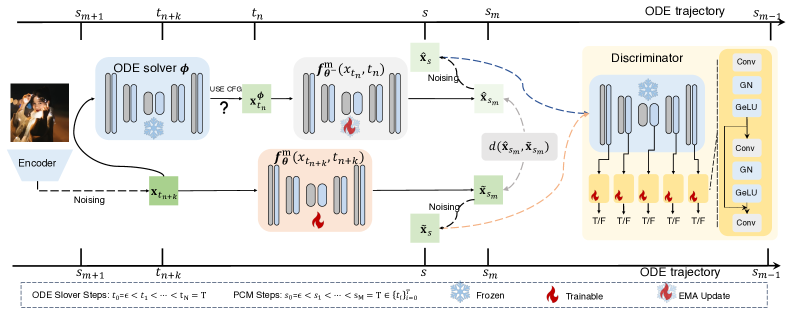
Figure 4: Training paradigm of PCM. ‘?’ means optional usage.

Definition. For a solution trajectory of a diffusion model {𝐱t}t[ϵ,T]subscriptsubscript𝐱𝑡𝑡italic-ϵ𝑇\{\mathbf{x}_{t}\}_{t\in[\epsilon,T]} following the PF-ODE, we split the trajectory into multiple sub-trajectories with hyper-defined edge timesteps s0,s1,,sMsubscript𝑠0subscript𝑠1subscript𝑠𝑀{s_{0},s_{1},\dots,s_{M}}, where s0=ϵsubscript𝑠0italic-ϵs_{0}=\epsilon and sM=Tsubscript𝑠𝑀𝑇s_{M}=T. The M𝑀M sub-trajectories can be represented as {𝐱t}t[sm,sm+1]subscriptsubscript𝐱𝑡𝑡subscript𝑠𝑚subscript𝑠𝑚1\{\mathbf{x}_{t}\}_{t\in[s_{m},s_{m+1}]} with m=0,1,,M1𝑚01𝑀1m=0,1,\dots,M-1. We treat each sub-trajectory as an independent CM and define the consistency function as 𝒇m:(𝐱t,t)𝐱sm,t[sm,sm+1]:superscript𝒇𝑚formulae-sequencesubscript𝐱𝑡𝑡subscript𝐱subscript𝑠𝑚𝑡subscript𝑠𝑚subscript𝑠𝑚1\bm{f}^{m}:(\mathbf{x}_{t},t)\rightarrow\mathbf{x}_{s_{m}},\quad t\in[s_{m},s_{m+1}]. We learn 𝒇θmsubscriptsuperscript𝒇𝑚𝜃\bm{f}^{m}_{\theta} to estimate 𝒇𝒇\bm{f} by enforcing the self-consistency property on each sub-trajectory that its outputs are consistent for arbitrary pairs on the same sub-trajectory. Namely, 𝒇m(𝐱t,t)=𝒇m(𝐱t,t)superscript𝒇𝑚subscript𝐱𝑡𝑡superscript𝒇𝑚subscript𝐱superscript𝑡superscript𝑡\bm{f}^{m}(\mathbf{x}_{t},t)=\bm{f}^{m}(\mathbf{x}_{t^{\prime}},t^{\prime}) for all t,t[sm,sm+1]𝑡superscript𝑡subscript𝑠𝑚subscript𝑠𝑚1t,t^{\prime}\in[s_{m},s_{m+1}]. Note that the consistency function is only defined on the sub-trajectory. However, for sampling, it is necessary to define a transition from timestep T𝑇T (i.e., sMsubscript𝑠𝑀s_{M}) to ϵitalic-ϵ\epsilon (i.e., s0subscript𝑠0s_{0}). Thereby, we defined 𝒇m,m=𝒇m(𝒇m2(𝒇m1(𝒇m(𝐱t,t),sm),sm1),sm)superscript𝒇𝑚superscript𝑚superscript𝒇superscript𝑚superscript𝒇𝑚2superscript𝒇𝑚1superscript𝒇𝑚subscript𝐱𝑡𝑡subscript𝑠𝑚subscript𝑠𝑚1subscript𝑠superscript𝑚\bm{f}^{m,m^{\prime}}=\bm{f}^{m^{\prime}}\left(\cdots\bm{f}^{m-2}\left(\bm{f}^{m-1}\left(\bm{f}^{m}(\mathbf{x}_{t},t\right),s_{m}),s_{m-1}\right)\cdots,s_{m^{\prime}}\right) that transforms any point 𝐱tsubscript𝐱𝑡\mathbf{x}_{t} on m𝑚m-th sub-trajectory to the solution point of msuperscript𝑚m^{\prime}-th trajectory.

Parameterization. Following the definition, each sub-trajectory, the corresponding consistency function satisfies 𝒇m(𝐱sm,sm)=𝐱smsuperscript𝒇𝑚subscript𝐱subscript𝑠𝑚subscript𝑠𝑚subscript𝐱subscript𝑠𝑚\bm{f}^{m}(\mathbf{x}_{s_{m}},s_{m})=\mathbf{x}_{s_{m}}, which is termed as boundary condition. The boundary condition is crucial for guaranteeing the successful training of consistency models. To satisfy the boundary condition, we typically need to explicitly parameterize 𝒇𝜽m(𝐱,t)superscriptsubscript𝒇𝜽𝑚𝐱𝑡\bm{f}_{\bm{\theta}}^{m}(\mathbf{x},t) as 𝒇𝜽m(𝐱,t)=cskipm(t)𝐱+coutm(t)F𝜽(𝐱,t,sm)superscriptsubscript𝒇𝜽𝑚𝐱𝑡subscriptsuperscript𝑐𝑚skip𝑡𝐱subscriptsuperscript𝑐𝑚out𝑡subscript𝐹𝜽𝐱𝑡subscript𝑠𝑚\bm{f}_{\bm{\theta}}^{m}(\mathbf{x},t)=c^{m}_{\text{skip}}(t)\mathbf{x}+c^{m}_{\text{out}}(t)F_{\bm{\theta}}(\mathbf{x},t,s_{m}), where cskipm(t)subscriptsuperscript𝑐𝑚skip𝑡c^{m}_{\text{skip}}(t) gradually increases to 111 and coutm(t)subscriptsuperscript𝑐𝑚out𝑡c^{m}_{\text{out}}(t) gradually decays to 0 from timestep sm+1subscript𝑠𝑚1s_{m+1} to smsubscript𝑠𝑚s_{m}.

Another important thing is how to parameterize F𝜽(𝐱,t,s)subscript𝐹𝜽𝐱𝑡𝑠F_{\bm{\theta}}(\mathbf{x},t,s), basically it should be able to indicate the target prediction at timestep s𝑠s given the input 𝐱𝐱\mathbf{x} at timestep t𝑡t. Since we build upon the epsilon prediction models, we hope to maintain the epsilon-prediction learning target.

For the above-discussed PF-ODE, there exists an exact solution [20] from timestep t𝑡t and s𝑠s

𝐱s=αsαt𝐱t+αsλtλseλσtλ(λ)logtλ(λ)(𝐱tλ(λ))dλsubscript𝐱𝑠subscript𝛼𝑠subscript𝛼𝑡subscript𝐱𝑡subscript𝛼𝑠superscriptsubscriptsubscript𝜆𝑡subscript𝜆𝑠superscript𝑒𝜆subscript𝜎subscript𝑡𝜆𝜆subscriptsubscript𝑡𝜆𝜆subscript𝐱subscript𝑡𝜆𝜆differential-d𝜆\mathbf{x}_{s}=\frac{\alpha_{s}}{\alpha_{t}}\mathbf{x}_{t}+\alpha_{s}\int_{\lambda_{t}}^{\lambda_{s}}e^{-\lambda}{\sigma_{t_{\lambda}(\lambda)}}\nabla\log\mathbb{P}_{t_{\lambda}(\lambda)}(\mathbf{x}_{t_{\lambda}(\lambda)})\mathrm{d}\lambda (2)

where λt=lnαtσtsubscript𝜆𝑡subscript𝛼𝑡subscript𝜎𝑡\lambda_{t}=\ln\frac{\alpha_{t}}{\sigma_{t}} and tλsubscript𝑡𝜆t_{\lambda} is a inverse function with λtsubscript𝜆𝑡\lambda_{t}. The equation shows that the solution of the ODE from t𝑡t to s𝑠s is the scaling of 𝐱tsubscript𝐱𝑡\mathbf{x}_{t} and the weighted sum of scores. Given a epsilon prediction diffusion network ϵϕ(𝐱,t)subscriptbold-italic-ϵbold-italic-ϕ𝐱𝑡\bm{\epsilon}_{\bm{\phi}}({\mathbf{x},t}), we can estimate the solution as 𝐱s=αsαt𝐱tαsλtλseλϵϕ(𝐱tλ(λ),tλ(λ))dλ.subscript𝐱𝑠subscript𝛼𝑠subscript𝛼𝑡subscript𝐱𝑡subscript𝛼𝑠superscriptsubscriptsubscript𝜆𝑡subscript𝜆𝑠superscript𝑒𝜆subscriptbold-italic-ϵbold-italic-ϕsubscript𝐱subscript𝑡𝜆𝜆subscript𝑡𝜆𝜆differential-d𝜆\mathbf{x}_{s}=\frac{\alpha_{s}}{\alpha_{t}}\mathbf{x}_{t}-\alpha_{s}\int_{\lambda_{t}}^{\lambda_{s}}e^{-\lambda}\bm{\epsilon}_{\bm{\phi}}(\mathbf{x}_{t_{\lambda}(\lambda)},t_{\lambda}(\lambda))\mathrm{d}\lambda. However, note that the solution requires knowing the epsilon prediction at each timestep, but consistency modes need to predict the solution with only 𝐱tsubscript𝐱𝑡\mathbf{x}_{t} available with one network evaluation. Thereby, we parameterize the F𝜽(𝐱,t,s)subscript𝐹𝜽𝐱𝑡𝑠F_{\bm{\theta}}(\mathbf{x},t,s) as following,

𝐱s=αsαt𝐱tαsϵ^θ(𝐱t,t)λtλseλdλ.subscript𝐱𝑠subscript𝛼𝑠subscript𝛼𝑡subscript𝐱𝑡subscript𝛼𝑠subscript^bold-italic-ϵ𝜃subscript𝐱𝑡𝑡superscriptsubscriptsubscript𝜆𝑡subscript𝜆𝑠superscript𝑒𝜆differential-d𝜆\mathbf{x}_{s}=\frac{\alpha_{s}}{\alpha_{t}}\mathbf{x}_{t}-\alpha_{s}\hat{\bm{\epsilon}}_{\theta}({\mathbf{x}_{t},t})\int_{\lambda_{t}}^{\lambda_{s}}e^{-\lambda}\mathrm{d}\lambda\,. (3)

One can show that the parameterization has the same format with DDIM 𝐱s=αs(𝐱tσtϵ𝜽(𝐱t,t)αt)+σsϵ𝜽(𝐱t,t)subscript𝐱𝑠subscript𝛼𝑠subscript𝐱𝑡subscript𝜎𝑡subscriptbold-italic-ϵ𝜽subscript𝐱𝑡𝑡subscript𝛼𝑡subscript𝜎𝑠subscriptbold-italic-ϵ𝜽subscript𝐱𝑡𝑡\mathbf{x}_{s}=\alpha_{s}(\frac{\mathbf{x}_{t}-\sigma_{t}\bm{\epsilon}_{\bm{\theta}}(\mathbf{x}_{t},t)}{\alpha_{t}})+\sigma_{s}\bm{\epsilon}_{\bm{\theta}}(\mathbf{x}_{t},t) (see Theorem 3). But here we clarify that the parameterization has a natural difference from DDIM. DDIM is the first-order approximation of solution ODE, which works because we assume the linearity of the score in small intervals. This causes the DDIM to degrade dramatically in a low-step regime since the linearity is no longer satisfied. But here, our parameterization is not approximation but exact solution learning. The learning target of ϵ^𝜽(𝐱,t)subscript^bold-italic-ϵ𝜽𝐱𝑡\hat{\bm{\epsilon}}_{\bm{\theta}}(\mathbf{x},t) is no more the scaled score σt𝐱logt(𝐱)subscript𝜎𝑡subscript𝐱subscript𝑡𝐱-\sigma_{t}\nabla_{\mathbf{x}}\log\mathbb{P}_{t}(\mathbf{x}) (which epsilon-prediction diffusion learned) but λtλseλϵϕ(𝐱tλ(λ),tλ(λ))dλλtλseλdλsuperscriptsubscriptsubscript𝜆𝑡subscript𝜆𝑠superscript𝑒𝜆subscriptbold-italic-ϵbold-italic-ϕsubscript𝐱subscript𝑡𝜆𝜆subscript𝑡𝜆𝜆differential-d𝜆superscriptsubscriptsubscript𝜆𝑡subscript𝜆𝑠superscript𝑒𝜆differential-d𝜆\frac{\int_{\lambda_{t}}^{\lambda_{s}}e^{-\lambda}\bm{\epsilon}_{\bm{\phi}}(\mathbf{x}_{t_{\lambda}(\lambda)},t_{\lambda}(\lambda))\mathrm{d}\lambda}{\int_{\lambda_{t}}^{\lambda_{s}}e^{-\lambda}\mathrm{d}\lambda} . Actually, we can define the parameterization in other formats, but we find this format is simple and has a small gap between the original diffusion models. The parameterization of Fθsubscript𝐹𝜃F_{\theta} also allows for a better property that we can drop the introduced cskipmsubscriptsuperscript𝑐𝑚skipc^{m}_{\text{skip}} and coutmsubscriptsuperscript𝑐𝑚outc^{m}_{\text{out}} in consistency models to ease the complexity of the framework. Note that following Eq. 3, we can get F𝜽(𝐱,sm,sm)=αsαs𝐱0=𝐱subscript𝐹𝜽𝐱subscript𝑠𝑚subscript𝑠𝑚subscript𝛼𝑠subscript𝛼𝑠𝐱0𝐱F_{\bm{\theta}}(\mathbf{x},s_{m},s_{m})=\frac{\alpha_{s}}{\alpha_{s}}\mathbf{x}-0=\mathbf{x}. Therefore, the boundary condition is already satisfied. Hence, we can simply define 𝒇𝜽m(𝐱,t)=F𝜽(𝐱,t,sm)subscriptsuperscript𝒇𝑚𝜽𝐱𝑡subscript𝐹𝜽𝐱𝑡subscript𝑠𝑚\bm{f}^{m}_{\bm{\theta}}(\mathbf{x},t)=F_{\bm{\theta}}(\mathbf{x},t,s_{m}).

Phased consistency distillation objective. Denote the pre-trained diffusion models as 𝒔ϕ(𝐱,t)=ϵϕ(𝐱,t)σtsubscript𝒔bold-italic-ϕ𝐱𝑡subscriptbold-italic-ϵbold-italic-ϕ𝐱𝑡subscript𝜎𝑡\bm{s}_{\bm{\phi}}(\mathbf{x},t)=-\frac{\bm{\epsilon}_{\bm{\phi}}(\mathbf{x},t)}{\sigma_{t}}, which induces an empirical PF-ODE. We firstly discretize the whole trajectory into N𝑁N sub-intervals with N+1𝑁1N+1 discrete timesteps from [ϵ,T]italic-ϵ𝑇[\epsilon,T], which we denote as t0=ϵ<t1<t2<<tN=Tsubscript𝑡0italic-ϵsubscript𝑡1subscript𝑡2subscript𝑡𝑁𝑇t_{0}=\epsilon<t_{1}<t_{2}<\cdots<t_{N}=T. Typically N𝑁N should be sufficiently large to make sure the ODE solver approximates the ODE trajectory correctly. Then we sample M+1𝑀1M+1 timesteps as edge timesteps s0=t0<s1<s2<<sM=tN{ti}i=0Nsubscript𝑠0subscript𝑡0subscript𝑠1subscript𝑠2subscript𝑠𝑀subscript𝑡𝑁superscriptsubscriptsubscript𝑡𝑖𝑖0𝑁s_{0}=t_{0}<s_{1}<s_{2}<\cdots<s_{M}=t_{N}\in\{t_{i}\}_{i=0}^{N} to split the ODE trajectory into M𝑀M sub-trajectories. Each sub-trajectory [si,si+1]subscript𝑠𝑖subscript𝑠𝑖1[s_{i},s_{i+1}] consists of the set of sub-intervals {[tj,tj+1]}tjsi,tj+1si+1subscriptsubscript𝑡𝑗subscript𝑡𝑗1formulae-sequencesubscript𝑡𝑗subscript𝑠𝑖subscript𝑡𝑗1subscript𝑠𝑖1\{[t_{j},t_{j+1}]\}_{t_{j}\geq s_{i},t_{j+1}\leq s_{i+1}}.

Here we define Φ(𝐱tn+k,tn+k,tn;ϕ)Φsubscript𝐱subscript𝑡𝑛𝑘subscript𝑡𝑛𝑘subscript𝑡𝑛bold-italic-ϕ\Phi(\mathbf{x}_{t_{n+k}},t_{n+k},t_{n};\bm{\phi}) as the k𝑘k-step ODE solver that approximate 𝐱tnϕsubscriptsuperscript𝐱bold-italic-ϕsubscript𝑡𝑛{\mathbf{x}}^{\bm{\phi}}_{t_{n}} from 𝐱tn+ksubscript𝐱subscript𝑡𝑛𝑘{\mathbf{x}}_{t_{n+k}} on the same sub-trajectory following Equation. 2, namely,

𝐱^tnϕ=Φ(𝐱tn+k,tn+k,tn;ϕ).subscriptsuperscript^𝐱bold-italic-ϕsubscript𝑡𝑛Φsubscript𝐱subscript𝑡𝑛𝑘subscript𝑡𝑛𝑘subscript𝑡𝑛bold-italic-ϕ\hat{\mathbf{x}}^{\bm{\phi}}_{t_{n}}=\Phi(\mathbf{x}_{t_{n+k}},t_{n+k},t_{n};\bm{\phi}). (4)

Following CM, we set k=1𝑘1k=1 to minimize the ODE solver cost. The training loss is defined as

PCM(𝜽,𝜽;ϕ)=𝔼(m),(n|m),(𝐱tn+1|n,m)[λ(tn)d(𝒇𝜽m(𝐱tn+1,tn+1),𝒇𝜽m(𝐱^tnϕ,tn))]subscriptPCM𝜽superscript𝜽bold-italic-ϕsubscript𝔼𝑚conditional𝑛𝑚conditionalsubscript𝐱subscript𝑡𝑛1𝑛𝑚delimited-[]𝜆subscript𝑡𝑛𝑑subscriptsuperscript𝒇𝑚𝜽subscript𝐱subscript𝑡𝑛1subscript𝑡𝑛1subscriptsuperscript𝒇𝑚superscript𝜽subscriptsuperscript^𝐱bold-italic-ϕsubscript𝑡𝑛subscript𝑡𝑛\mathcal{L}_{\text{PCM}}(\bm{\theta},\bm{\theta}^{-};\bm{\phi})=\mathbb{E}_{\mathbb{P}(m),\mathbb{P}(n|m),\mathbb{P}({\mathbf{x}_{t_{n+1}}|n,m})}\left[\lambda(t_{n})d\left(\bm{f}^{m}_{\bm{\theta}}(\mathbf{x}_{t_{n+1}},t_{n+1}),\bm{f}^{m}_{\bm{\theta}^{-}}(\hat{\mathbf{x}}^{\bm{\phi}}_{t_{n}},t_{n})\right)\right] (5)

where (m):=uniform({0,1,,M1})assign𝑚uniform01𝑀1\mathbb{P}(m):=\mathrm{uniform(}{\{0,1,\dots,M-1}\}), (n|m):=uniform({n+1|tn+1sm+1,tnsm})assignconditional𝑛𝑚uniformconditional-set𝑛1formulae-sequencesubscript𝑡𝑛1subscript𝑠𝑚1subscript𝑡𝑛subscript𝑠𝑚\mathbb{P}(n|m):=\text{uniform}(\{n+1|t_{n+1}\leq s_{m+1},t_{n}\geq s_{m}\}), (𝐱tn+1|n,m)=tn+1(𝐱)conditionalsubscript𝐱subscript𝑡𝑛1𝑛𝑚subscriptsubscript𝑡𝑛1𝐱\mathbb{P}(\mathbf{x}_{t_{n+1}}|n,m)=\mathbb{P}_{t_{n+1}}(\mathbf{x}), and 𝜽=μ𝜽+(1μ)𝜽superscript𝜽𝜇superscript𝜽1𝜇𝜽\bm{\theta}^{-}=\mu\bm{\theta}^{-}+(1-\mu)\bm{\theta}.

We show that when PCM(𝜽,𝜽;ϕ)=0subscriptPCM𝜽superscript𝜽bold-italic-ϕ0\mathcal{L}_{\text{PCM}}(\bm{\theta},\bm{\theta}^{-};\bm{\phi})=0 and local errors of ODE solvers uniformly bounded by 𝒪((Δt)p+1)𝒪superscriptΔ𝑡𝑝1\mathcal{O}((\Delta t)^{p+1}), the solution estimation error within the arbitrary sub-trajectory 𝒇𝜽m(𝐱tn,tn)superscriptsubscript𝒇𝜽𝑚subscript𝐱subscript𝑡𝑛subscript𝑡𝑛\bm{f}_{\bm{\theta}}^{m}(\mathbf{x}_{t_{n}},t_{n}) is bounded by 𝒪((Δt)p)𝒪superscriptΔ𝑡𝑝\mathcal{O}((\Delta t)^{p}) in Theorem 1. Additionally, the solution estimation error across any sets of sub-trajectories (i.e., the error between 𝒇𝜽m,m(𝐱tn,tn)superscriptsubscript𝒇𝜽𝑚superscript𝑚subscript𝐱subscript𝑡𝑛subscript𝑡𝑛\bm{f}_{\bm{\theta}}^{m,m^{\prime}}(\mathbf{x}_{t_{n}},t_{n}) and 𝒇m,m(𝐱tn+1,tn+1;ϕ)superscript𝒇𝑚superscript𝑚subscript𝐱subscript𝑡𝑛1subscript𝑡𝑛1bold-italic-ϕ\bm{f}^{m,m^{\prime}}(\mathbf{x}_{t_{n+1},t_{n+1}};\bm{\phi})) is also bounded by 𝒪((Δt)p)𝒪superscriptΔ𝑡𝑝\mathcal{O}((\Delta t)^{p}) in Theorem 2.

Sampling. For a given initial sample at timestep t𝑡t which belongs to the sub-trajectory [sm,sm+1]subscript𝑠𝑚subscript𝑠𝑚1[s_{m},s_{m+1}], we can support deterministic sampling following the definition of 𝒇m,0superscript𝒇𝑚0\bm{f}^{m,0}. Previous work [12, 40] reveals that introducing a certain degree of stochasticity might lead to better generation results. We show that our sampling method can also introduce randomness through a simple modification, which we discuss at Sec. IV.1

3.2 Guided-Distillation
Refer to caption

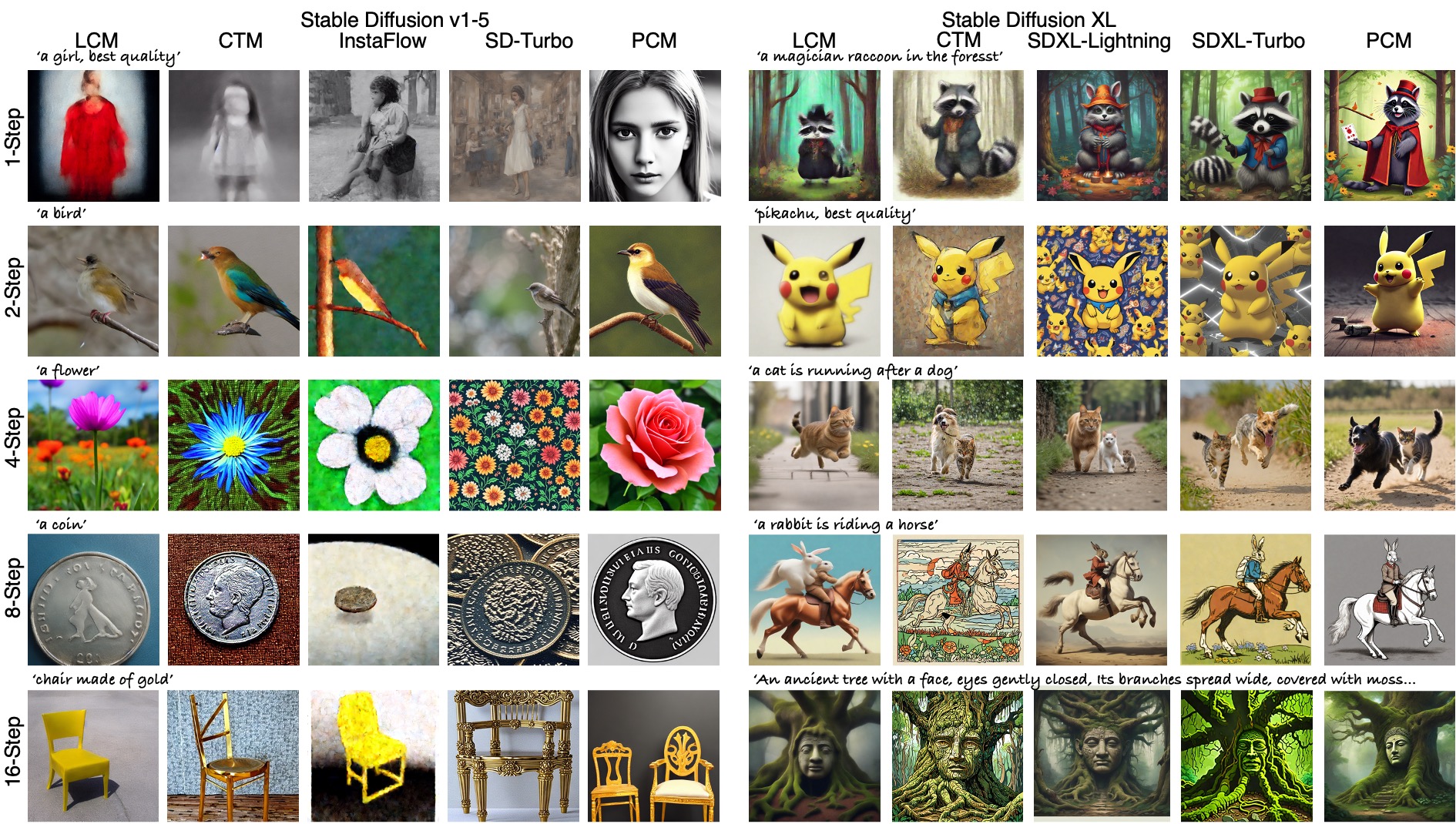
Figure 5: Qualitative Comparison. Our method achieves top performance.

For convenience, we take the epsilon-prediction format with text conditions 𝒄𝒄\bm{c} for discussion. The consistency model is denoted as ϵ𝜽(𝐱,t,𝒄)subscriptbold-italic-ϵ𝜽𝐱𝑡𝒄\bm{\epsilon}_{\bm{\theta}}(\mathbf{x},t,\bm{c}), and the diffusion model is denoted as ϵϕ(𝐱,t,𝒄)subscriptbold-italic-ϵbold-italic-ϕ𝐱𝑡𝒄\bm{\epsilon}_{\bm{\phi}}(\mathbf{x},t,\bm{c}). A commonly applied strategy for text-conditioned diffusion models is classifier-free guidance (CFG). At training, they randomly substitute 𝒄𝒄\bm{c} with null text embedding \varnothing. At each inference step, the model compute ϵϕ(𝐱,t,𝒄)subscriptbold-italic-ϵbold-italic-ϕ𝐱𝑡𝒄\bm{\epsilon}_{\bm{\phi}}(\mathbf{x},t,\bm{c}) and ϵϕ(𝐱,t,𝒄neg)subscriptbold-italic-ϵbold-italic-ϕ𝐱𝑡subscript𝒄neg\bm{\epsilon}_{\bm{\phi}}(\mathbf{x},t,\bm{c}_{\text{neg}}) simultaneously, and the actual prediction is the linear combination of them. Namely,

ϵϕ(𝐱,t,𝒄,𝒄neg;w)=ϵϕ(𝐱,t,𝒄neg)+w(ϵϕ(𝐱,t,𝒄)ϵϕ(𝐱,t,𝒄neg)),subscriptbold-italic-ϵitalic-ϕ𝐱𝑡𝒄subscript𝒄neg𝑤subscriptbold-italic-ϵbold-italic-ϕ𝐱𝑡subscript𝒄neg𝑤subscriptbold-italic-ϵbold-italic-ϕ𝐱𝑡𝒄subscriptbold-italic-ϵbold-italic-ϕ𝐱𝑡subscript𝒄neg\bm{\epsilon}_{\phi}(\mathbf{x},t,\bm{c},\bm{c}_{\text{neg}};w)=\bm{\epsilon}_{\bm{\phi}}(\mathbf{x},t,\bm{c}_{\text{neg}})+w(\bm{\epsilon}_{\bm{\phi}}(\mathbf{x},t,\bm{c})-\bm{\epsilon}_{\bm{\phi}}(\mathbf{x},t,\bm{c}_{\text{neg}})), (6)

where w𝑤w controlling the strength and 𝒄negsubscript𝒄neg\bm{c}_{\text{neg}} can be set to \varnothing or text embeddings of unwanted characteristics. A noticeable phenomenon is that models with this strategy can not generate content with good quality without using CFG. That is, the ODE trajectory induced with pure ϵϕ(𝐱,t,𝒄)subscriptbold-italic-ϵbold-italic-ϕ𝐱𝑡𝒄\bm{\epsilon}_{\bm{\phi}}(\mathbf{x},t,\bm{c}) deviates away from the ODE trajectory to real data distribution. Thereby, it is necessary to apply CFG-augmented prediction ϵϕ(𝐱,t,𝒄,𝒄neg;w)subscriptbold-italic-ϵbold-italic-ϕ𝐱𝑡𝒄subscript𝒄neg𝑤\bm{\epsilon}_{\bm{\phi}}(\mathbf{x},t,\bm{c},\bm{c}_{\text{neg}};w) for ODE solvers. Recall that we have shown that the consistency learning target of the consistency model ϵ𝜽(𝐱,t,𝒄)subscriptbold-italic-ϵ𝜽𝐱𝑡𝒄\bm{\epsilon}_{\bm{\theta}}(\mathbf{x},t,\bm{c}) is the weighted sum of epsilon prediction on the trajectory. Thereby, we have ϵ𝜽(𝐱,t,𝒄)ϵϕ(𝐱,t,𝒄,;w),proportional-tosubscriptbold-italic-ϵ𝜽𝐱𝑡𝒄subscriptbold-italic-ϵitalic-ϕ𝐱superscript𝑡𝒄𝑤\bm{\epsilon}_{\bm{\theta}}(\mathbf{x},t,\bm{c})\propto\bm{\epsilon}_{\phi}(\mathbf{x},t^{\prime},\bm{c},\varnothing;w), for all ttsuperscript𝑡𝑡t^{\prime}\leq t. On this basis, if we additionally apply the CFG for the consistency models, we can prove that

ϵ𝜽(𝐱,t,𝒄,𝒄neg;w)ww(ϵϕ(𝐱,t,𝒄)ϵϕmerge))+ϵϕ(𝐱,t,𝒄neg),\displaystyle\bm{\epsilon}_{\bm{\theta}}(\mathbf{x},t,\bm{c},\bm{c}_{\text{neg}};w^{\prime})\propto ww^{\prime}(\bm{\epsilon}_{\bm{\phi}}(\mathbf{x},t,\bm{c})-\bm{\epsilon}_{\bm{\phi}}^{\text{merge}}))+\bm{\epsilon}_{\bm{\phi}}(\mathbf{x},t,\bm{c}_{\text{neg}})\,, (7)

where ϵϕmerge=(1α)ϵϕ(𝐱,t,𝒄neg)+αϵϕ(𝐱,t,)superscriptsubscriptbold-italic-ϵbold-italic-ϕmerge1𝛼subscriptbold-italic-ϵbold-italic-ϕ𝐱𝑡subscript𝒄neg𝛼subscriptbold-italic-ϵbold-italic-ϕ𝐱𝑡\bm{\epsilon}_{\bm{\phi}}^{\text{merge}}=(1-\alpha)\bm{\epsilon}_{\bm{\phi}}(\mathbf{x},t,\bm{c}_{\text{neg}})+\alpha\bm{\epsilon}_{\bm{\phi}}(\mathbf{x},t,\varnothing) andα=(w1)ww𝛼𝑤1𝑤superscript𝑤\alpha=\frac{(w-1)}{ww^{\prime}} (See Theorem 4). This equation indicates that applying CFG wsuperscript𝑤w^{\prime} to the consistency models with guided distillation confined with w𝑤w, is equivalent to scaling the prediction of original diffusion models by wwsuperscript𝑤𝑤w^{\prime}w, which explains the the exposure problem. We can also observe that the epsilon prediction with negative prompts is diluted by the prediction with null text embedding, which reveals that the impact of negative prompts is reduced.

We ask the question: Is it possible to conduct consistency distillation with diffusion models trained for CFG usage without applying CFG-augmented ODE solver? Our finding is that it is not applicable for original CM but works well for PCM especially when the number of sub-trajectory M𝑀M is large. We empirically find that M=4𝑀4M=4 is sufficient for successful training. As we discussed, the text-conditioned diffusion models trained for CFG fail at achieving good generation quality when removing CFG for inference. That is, target data distribution induced by PF-ODE with ϵϕ(𝐱,t,𝒄)subscriptbold-italic-ϵbold-italic-ϕ𝐱𝑡𝒄\bm{\epsilon}_{\bm{\phi}}(\mathbf{x},t,\bm{c}) has a large distribution distance to real data distribution. Therefore, fitting the spoiled ODE trajectory is only to make the generation quality bad. In contrast, when phasing the whole ODE trajectory into several sub-trajectories, the negative influence is greatly alleviated. On one hand, the starting point (𝐱sm+1subscript𝐱subscript𝑠𝑚1\mathbf{x}_{s_{m+1}}) of sub-trajectories is replaced by adding noise to the real data. On the other hand, the distribution distance between the distribution of solution points (𝐱smsubscript𝐱subscript𝑠𝑚\mathbf{x}_{s_{m}}) of sub-trajectories and real data distribution smdatasuperscriptsubscriptsubscript𝑠𝑚data\mathbb{P}_{s_{m}}^{\text{data}} at the same timestep is much smaller proportional to the noise level introduced. To put it straightforwardly, even though the distribution distance between the real data and the samples generated from ϵϕ(𝐱,t,𝒄)subscriptbold-italic-ϵbold-italic-ϕ𝐱𝑡𝒄\bm{\epsilon}_{\bm{\phi}}(\mathbf{x},t,\bm{c}) is large, adding noise to them reduce the gap. Thereby, we can optionally train a consistency model whether supporting larger CFG values or not.

3.3 Adversarial Consistency Loss

We introduce an adversarial loss to enforce the distribution consistency, which greatly improves the generation results in low-step regime. For convenience, we introduce additional symbol 𝒯tssubscript𝒯𝑡𝑠\mathcal{T}_{t\to s} which represents a flow from tsubscript𝑡\mathbb{P}_{t} to ssubscript𝑠\mathbb{P}_{s}. Let 𝒯tsϕsubscriptsuperscript𝒯bold-italic-ϕ𝑡𝑠\mathcal{T}^{\bm{\phi}}_{t\to s}, 𝒯ts𝜽superscriptsubscript𝒯𝑡𝑠𝜽\mathcal{T}_{t\to s}^{\bm{\theta}} be the transition mapping following the ODE trajectory of pre-trained diffusion and our consistency models. Additionally, let 𝒯stsubscriptsuperscript𝒯𝑠𝑡\mathcal{T}^{-}_{s\to t} be the distribution transition following the forward process SDE (adding noise). The loss function is defined as the following

PCMadv(𝜽,𝜽;ϕ,m)=D(𝒯sms𝒯tn+ksm𝜽#tn+k𝒯sms𝒯tnsm𝜽𝒯tn+1tnϕ#tn+1),\mathcal{L}^{adv}_{\text{PCM}}(\bm{\theta},\bm{\theta}^{-};\bm{\phi},m)=D\left(\mathcal{T}^{-}_{s_{m}\to s}\mathcal{T}^{\bm{\theta}}_{t_{n+k}\to s_{m}}\#\mathbb{P}_{t_{n+k}}\middle\|\mathcal{T}^{-}_{s_{m}\to s}\mathcal{T}^{\bm{\theta}^{-}}_{t_{n}\to s_{m}}\mathcal{T}^{\bm{\phi}}_{t_{n+1}\to t_{n}}\#\mathbb{P}_{t_{n+1}}\right)\,, (8)

where ##\# is the pushforward operator, and D𝐷D is the distribution distance metric. To penalize the distribution distance, we apply the GAN-style training paradigm. To be specific, as shown in Fig. 4, for the sampled 𝐱tn+ksubscript𝐱subscript𝑡𝑛𝑘\mathbf{x}_{t_{n+k}} and the 𝐱tnϕsuperscriptsubscript𝐱subscript𝑡𝑛bold-italic-ϕ\mathbf{x}_{t_{n}}^{\bm{\phi}} solved through the pre-trained diffusion model ϕbold-italic-ϕ\bm{\phi}, we first compute their predicted solution point 𝐱~sm=𝒇𝜽m(𝐱tn+k,tn+k)subscript~𝐱subscript𝑠𝑚superscriptsubscript𝒇𝜽𝑚subscript𝐱subscript𝑡𝑛𝑘subscript𝑡𝑛𝑘\tilde{\mathbf{x}}_{s_{m}}=\bm{f}_{\bm{\theta}}^{m}(\mathbf{x}_{t_{n+k}},t_{n+k}) and 𝐱^sm=𝒇𝜽(𝐱tnϕ,tn)subscript^𝐱subscript𝑠𝑚subscript𝒇superscript𝜽superscriptsubscript𝐱subscript𝑡𝑛bold-italic-ϕsubscript𝑡𝑛\hat{\mathbf{x}}_{s_{m}}=\bm{f}_{\bm{\theta^{-}}}(\mathbf{x}_{t_{n}}^{\bm{\phi}},t_{n}). Then we randomly add noise to 𝐱~smsubscript~𝐱subscript𝑠𝑚\tilde{\mathbf{x}}_{s_{m}} and 𝐱^smsubscript^𝐱subscript𝑠𝑚\hat{\mathbf{x}}_{s_{m}} to obtain 𝐱~ssubscript~𝐱𝑠\tilde{\mathbf{x}}_{s} and 𝐱^ssubscript^𝐱𝑠\hat{\mathbf{x}}_{s} with randomly sampled s[sm,sm+1]𝑠subscript𝑠𝑚subscript𝑠𝑚1s\in[s_{m},s_{m+1}]. We optimize the adversarial loss between 𝐱~ssubscript~𝐱𝑠\tilde{\mathbf{x}}_{s} and 𝐱^ssubscript^𝐱𝑠\hat{\mathbf{x}}_{s}. Specifically, the PCMadvsuperscriptsubscriptPCM𝑎𝑑𝑣\mathcal{L}_{\text{PCM}}^{adv} can be re-written as

PCMadv(𝜽,𝜽;ϕ,m)=ReLU(1+𝐱~s)+ReLU(1𝐱^s),superscriptsubscriptPCM𝑎𝑑𝑣𝜽superscript𝜽bold-italic-ϕ𝑚ReLU1subscript~𝐱𝑠ReLU1subscript^𝐱𝑠\mathcal{L}_{\text{PCM}}^{adv}(\bm{\theta},\bm{\theta}^{-};\bm{\phi},m)=\text{ReLU}(1+\tilde{\mathbf{x}}_{s})+\text{ReLU}(1-\hat{\mathbf{x}}_{s}), (9)

where ReLU(x)=xReLU𝑥𝑥\text{ReLU}(x)=x if x>0𝑥0x>0 else ReLU(x)=0ReLU𝑥0\text{ReLU}(x)=0, and the loss is updated in a minmax manner. Therefore the eventual optimization objective is PCM+λPCMadvsubscriptPCM𝜆superscriptsubscriptPCM𝑎𝑑𝑣\mathcal{L}_{\text{PCM}}+\lambda\mathcal{L}_{\text{PCM}}^{adv} with λ𝜆\lambda as a hyper-parameter controlling the trade-off of distribution consistency and instance consistency.. However, we hope to clarify that the adversarial loss has an intrinsic difference from the GAN. The GAN training aims to align the training data distribution and the generation distribution of the model. That is, D(𝒯tn+ksm𝜽#tn+ksm)𝐷conditionalsubscriptsuperscript𝒯𝜽subscript𝑡𝑛𝑘subscript𝑠𝑚#subscriptsubscript𝑡𝑛𝑘subscriptsubscript𝑠𝑚D(\mathcal{T}^{\bm{\theta}}_{t_{n+k}\to s_{m}}\#\mathbb{P}_{t_{n+k}}\|\mathbb{P}_{s_{m}}) In Theorem 5, we show that consistency property is enforced, our introduced adversarial loss will also coverage to zero. Yet in Theorem 6, we show that combining standard GAN with consistency distillation is a flawed design when considering the pre-trained data distribution and distillation data distribution mismatch. Its loss will be non-zero when the self-consistency property is achieved, thus corrupting the consistency distillation learning. Our experimental results also verify our statement (Fig. 8).

4 Experiments

4.1 Experimental Setup

Dataset. Training dataset: For image generation, we train all models on the CC3M [3] dataset. For video generation, we train the model on WebVid-2M [1]. Evaluation dataset: For image generation, we evaluate the performance on the COCO-2014 [17] following the 30K split of karpathy. We also evaluate the performance on the CC12M (excluding the CC3M) with our randomly chosen 30K split. For video generation, we evaluate with the captions of UCF-101 [37].

Backbones. We verify the text-to-image generation based on Stable Diffusion v1-5 [27] and Stable Diffusion XL [24]. We verify the text-to-video generation following the design of AnimateLCM with decoupled consistency distillation.

Evaluation metrics. Image: We report the FID [8] and CLIP score [26] of the generated images and the validation 30K-sample splits. Following  [6, 29], we also compute the FID with CLIP features (FID-CLIP). Note that, all baselines and our method focus on distilling the knowledge from the pre-trained diffusion models for acceleration. Therefore, we also compute the FID of all baselines and the generated images of original pre-trained diffusion models including Stable Diffusion v1-5 and Stable Diffusion XL (FID-SD). Video: For video generation, we evaluate the performance from three perspectives: the CLIP Score to measure the text-video alignment, the CLIP Consistency to measure the inter-frame consistency of the generated videos, the Flow Magnitude to measure the motion magnitude of the generated videos with Raft-Large [38].

4.2 Comparison

Comparison methods. We compare PCM with Stable Diffusion v1-5 to methods including Stable Diffusion v1-5 [27], InstaFlow [19], LCM [21], CTM [12], and SD-Turbo [31]. We compare PCM with Stable Diffusion XL to methods including Stable Diffusion XL [24], CTM [12], SDXL-Lightning [16], SDXL-Turbo [31], and LCM [21]. We apply the ‘Ours’ and ‘Ours*’ to denote our methods trained with CFG-Augmented ODE solver or not. We only report the performance of ‘Ours*’ with more than 4 steps which aligns with our claim that it is only possible when phasing the ODE trajectory into multiple sub-trajectories. For video generation, we compare with DDIM [33], DPM [20], and AnimateLCM [39].

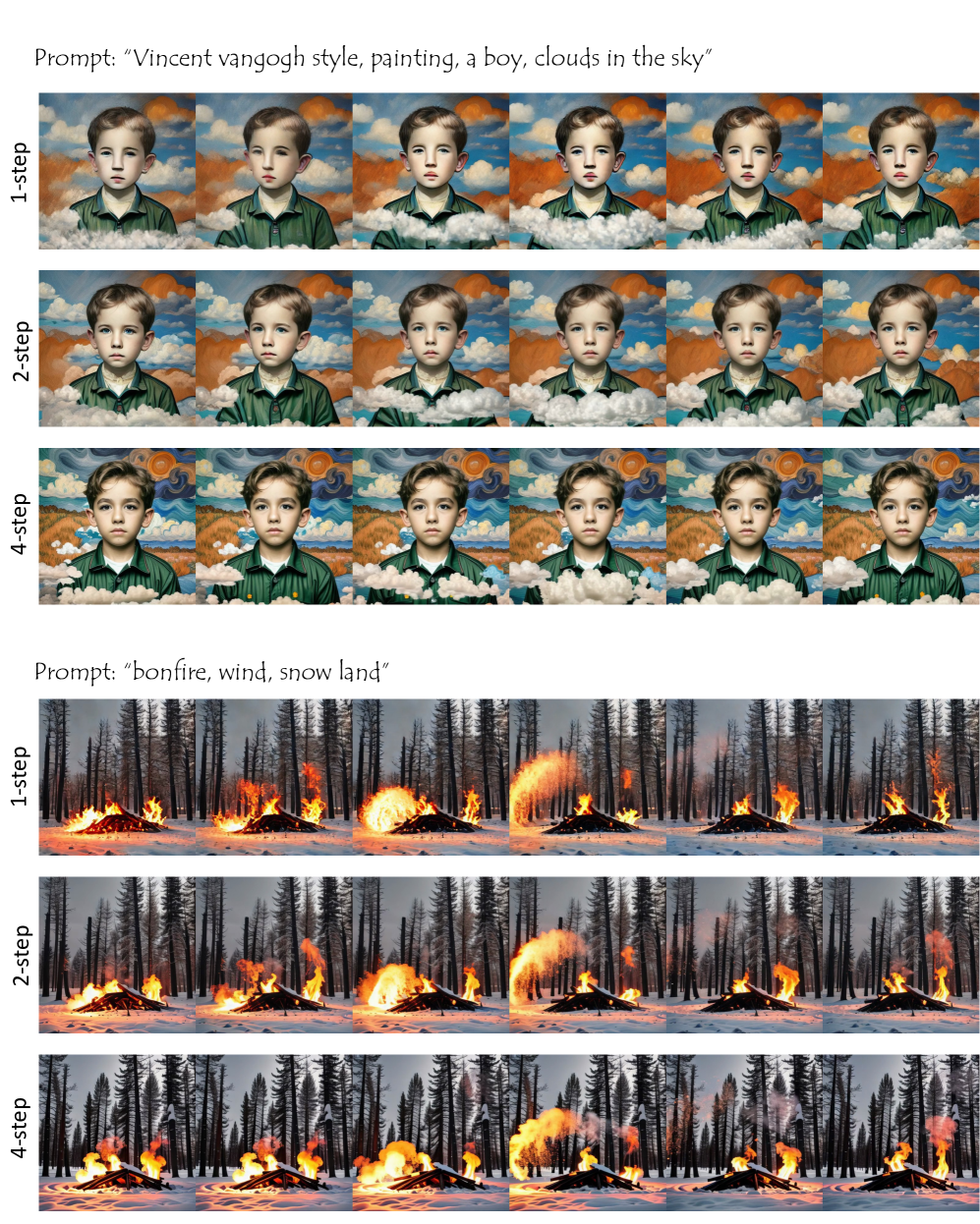
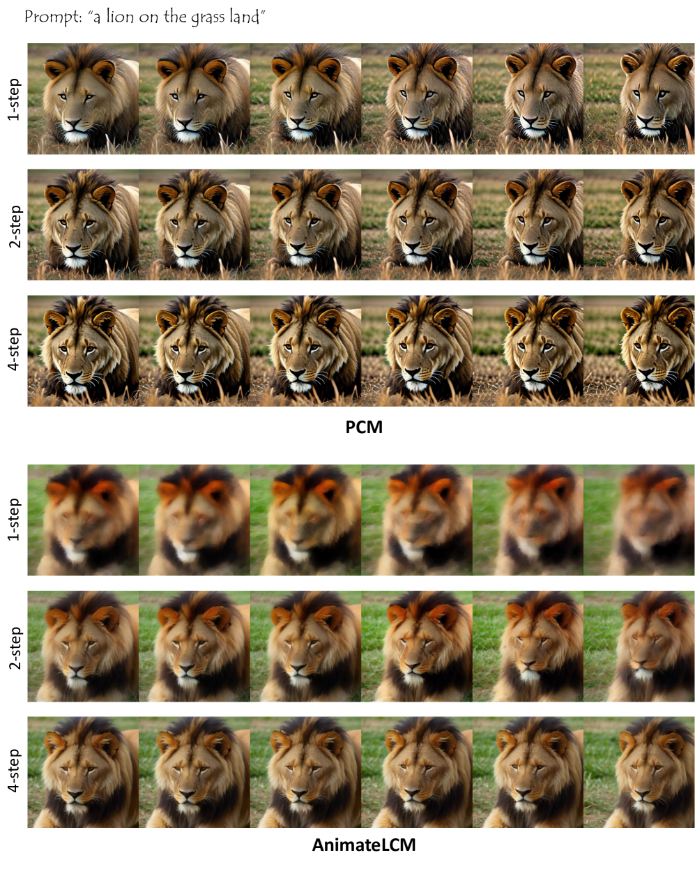
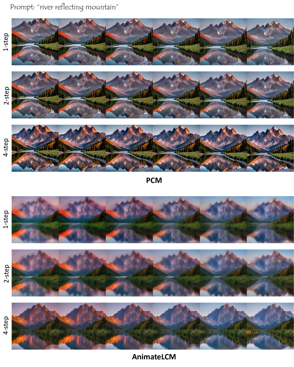
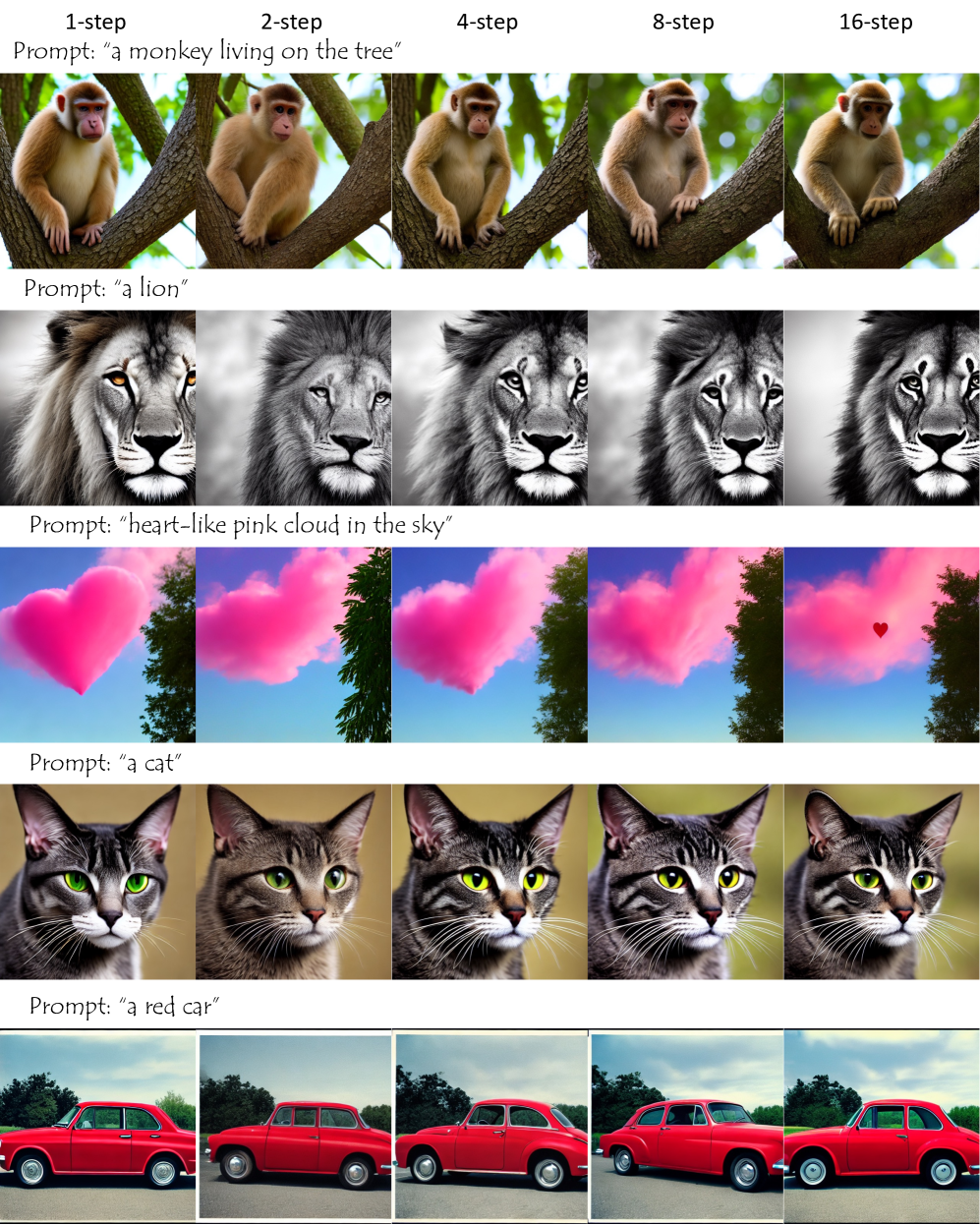
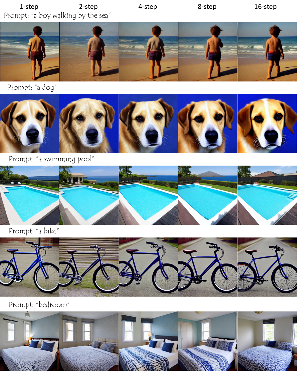
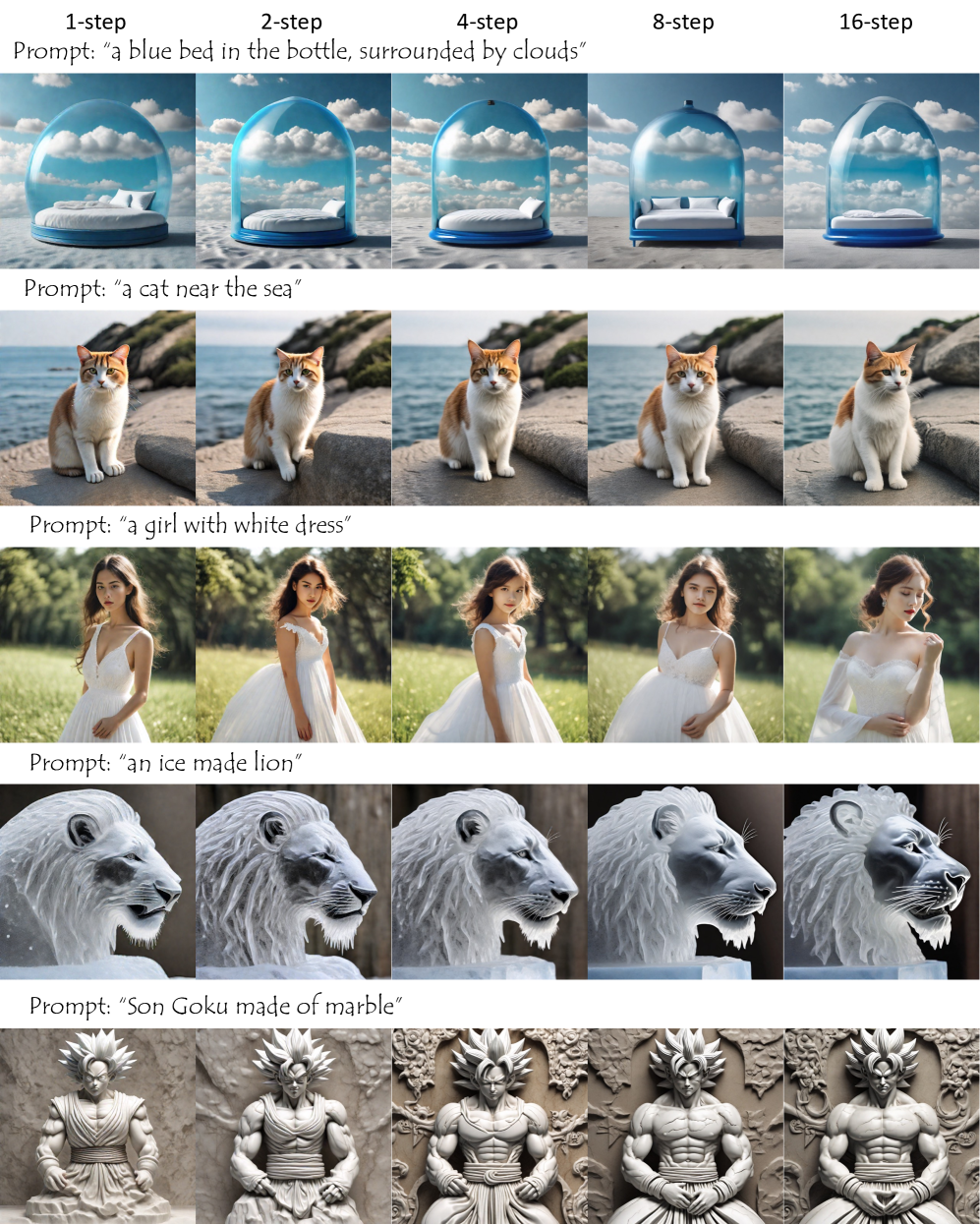
Qualitative comparison. We evaluate our model and comparison methods with a diverse set of prompts in different inference steps. The results are listed in Fig. 5. Our method shows clearly the top performance in both image visual quality and text-image alignment across 1-16 steps.

Quantitative comparison. One-step generation: We show the one-step generation results comparison of methods based on Stable Diffusion v1-5 and Stable Diffusion XL in Table. 2 and Table. 5, respectively. Notably, PCM consistently surpasses the consistency model-based methods including LCM and CTM by a large margin. Additionally, it achieves comparable or even superior to the state-of-the-art GAN-based (SD-Turbo, SDXL-Turbo, SDXL-Lightning) or Rectified-Flow-based (InstaFlow) one-step generation methods. Note that InstaFlow applies the LIPIPS [42] loss for training and SDXL-Turbo can only generate 512×512512512512\times 512 resolution images, therefore it is easy for them to obtain higher scores. Multi-step generation: We report the FID changes of different methods on COCO-30K and CC12M-30K in Table 1 and Table 4. ‘Ours’ and ‘Ours*’ achieve the best or second-best performance in most cases. It is notably the gap of performance between our methods and other baselines becoming large as the timestep increases, which indicates the phased nature of our methods supports more powerful multi-step sampling ability. Video generation: We show the quantitative comparison of video generation in Table 4, our model achieves consistent superior performance. The 1-step and 2-step generation results of DDIM and DPM are very noisy, therefore it is meaningless to evaluate their Flow Magnitude and CLIP Consistency.

Table 1: Comparison of FID-SD and FID-CLIP with Stable Diffusion v1-5 based methods under different steps.
METHODS FID-SD FID-CLIP
COCO-30K CC12M-30K COCO-30K
1 2 4 8 16 1 2 4 8 16 1 2 4 8 16
InstaFlow [19] 11.51 69.79 102.15 122.20 139.29 11.90 62.48 88.64 105.34 113.56 9.56 29.38 38.24 43.60 47.32
SD-Turbo [31] 10.62 12.22 16.66 24.30 30.32 10.35 12.03 15.15 19.91 23.34 12.08 15.07 15.12 14.90 15.09
LCM [21] 53.43 11.03 6.66 6.62 7.56 42.67 10.51 6.40 5.99 9.02 21.04 10.18 10.64 12.15 13.85
CTM [12] 63.55 9.93 9.30 15.62 21.75 28.47 8.98 8.22 13.27 17.43 30.39 10.32 10.31 11.27 12.75
Ours 8.27 9.79 5.81 5.00 4.70 7.91 8.93 4.93 3.88 3.85 11.66 9.17 9.07 9.49 10.13
Ours* - - 7.46 6.49 5.78 - - 4.99 5.01 5.13 - - 8.85 8.33 8.09
Table 2: One-step generation comparison on Stable Diffusion v1-5.
METHODS COCO-30K CC12M-30K CONSISTENCY \uparrow
FID \downarrow FID-CLIP \downarrow FID-SD \downarrow CLIP SCORE \uparrow FID \downarrow FID-CLIP \downarrow FID-SD \downarrow CLIP SCORE \uparrow
InstaFlow [19] 13.59 9.56 11.51 29.37 15.06 6.16 11.90 24.52 0.61
SD-Turbo [31] 16.56 12.08 10.62 31.21 17.17 6.18 12.48 26.30 0.71
CTM [12] 67.55 30.39 63.55 23.98 56.39 28.47 28.47 18.81 0.65
LCM [21] 53.81 21.04 53.43 25.23 44.35 18.58 42.67 20.38 0.62
Ours 17.91 11.66 8.27 29.26 14.79 5.38 7.91 26.33 0.81
Table 3: Comparison of FID-SD on CC12M-30K with Stable Diffusion XL.
METHODS 1-Step 2-Step 4-Step 8-Step 16-Step
SDXL-Lightning [16] 8.69 7.29 5.26 5.83 6.10
SDXL-Turbo (512×512512512512\times 512[31] 6.64 6.53 7.39 13.88 26.55
SDXL-LCM [21] 57.70 19.64 11.22 12.89 23.33
SDXL-CTM [12] 72.45 24.06 20.67 39.89 39.18
Ours 8.76 7.02 6.59 5.19 4.92
Ours* - - 6.26 5.27 5.09
Table 4: Quantitative comparison for video generation.
Methods CLIP Score \uparrow Flow Magnitude \uparrow CLIP Consistency \uparrow
1-Step 2-Step 4-Step 1-Step 2-Step 4-Step 1-Step 2-Step 4-Step
DDIM [33] 4.44 7.09 23.05 - - 1.47 - - 0.877
DPM [20] 11.21 17.93 28.57 - - 1.95 - - 0.947
AnimateLCM [39] 25.41 29.39 30.62 1.10 1.81 2.40 0.967 0.957 0.965
Ours 29.88 30.22 30.72 4.56 4.38 4.69 0.956 0.962 0.968
Table 5: One-step and two-step generation comparison on Stable Diffusion XL.
METHODS COCO-30K (one-step) CC12M-30K (two-step) CONSISTENCY \uparrow
FID \downarrow FID-CLIP \downarrow FID-SD \downarrow CLIP SCORE \uparrow FID \downarrow FID-CLIP \downarrow FID-SD \downarrow CLIP SCORE \uparrow
SDXL Turbo (512×512512512512\times 512[31] 19.84 13.56 9.40 32.31 15.36 5.26 6.53 27.91 0.74
SDXL Lightning [16] 19.73 13.33 9.11 30.81 17.99 7.39 7.29 26.31 0.76
SDXL LCM [21] 74.65 31.63 74.46 27.29 25.88 10.36 19.64 25.84 0.66
SDXL CTM [12] 82.14 37.43 88.20 26.48 32.05 12.50 24.06 24.79 0.66
Ours 21.23 13.66 9.32 31.55 17.87 5.67 7.02 27.10 0.83

4.3 Ablation Study

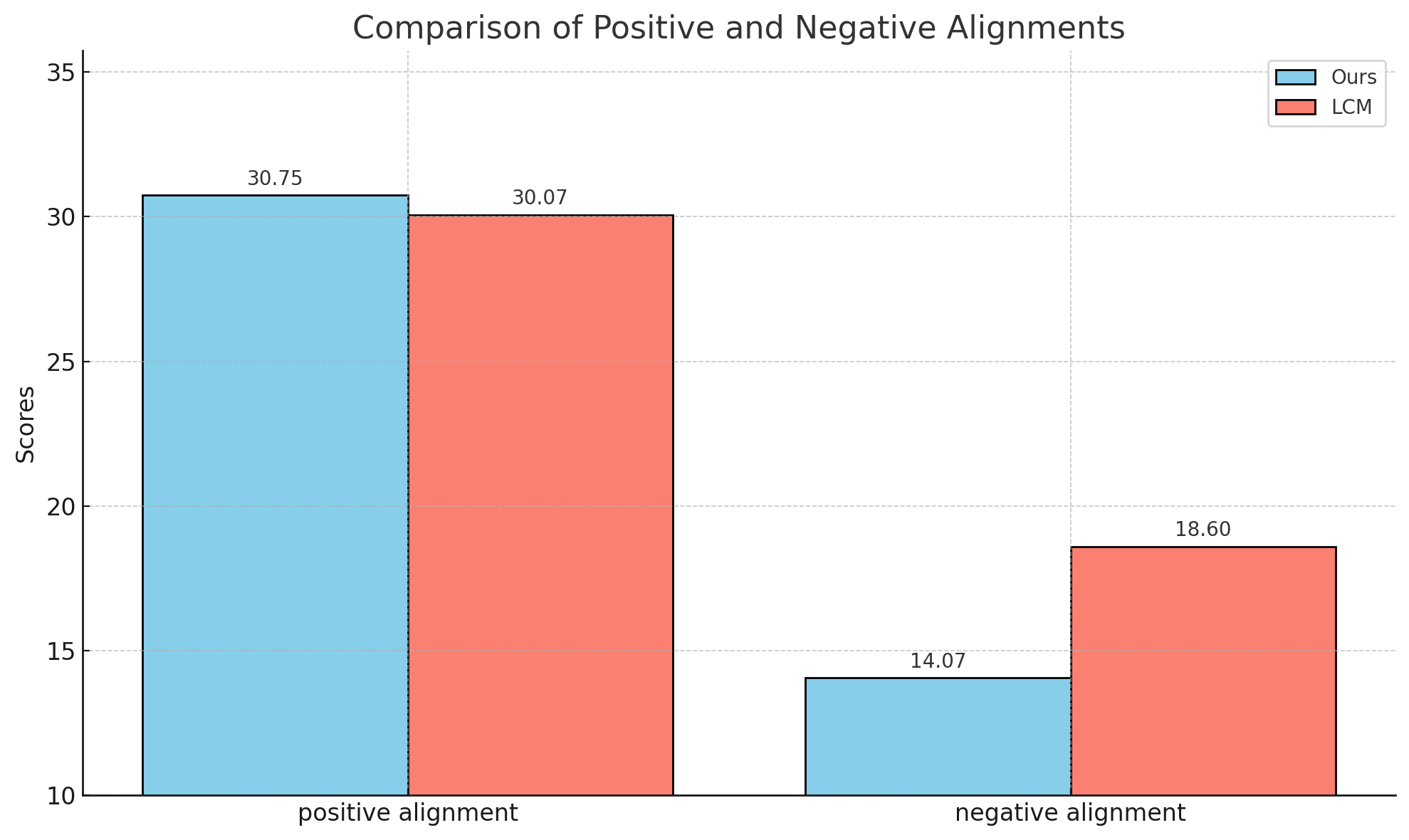
Sensitivity to negative prompt. To show the comparison of sensitivity to negative prompt between our model tuned without CFG-Augmented ODE solver and LCM. We provide an example of a prompt and negative prompt to GPT-4o and ask it to generate 100 pairs of prompts and their corresponding negative prompts. For each prompt, we generate 10 images. We first generate images without using the negative prompt to show the positive prompt alignment comparison. Then we generate images with positive and negative prompts. We compute the CLIP score of generated images and the prompts and negative prompts. Fig. 8 shows that we not only achieve better prompt alignment but are much more sensitive to negative prompts.

Consistent generation ability. Consistent generation ability under different inference steps is valuable in practice for multistep refinement. We compute the average CLIP similarity between the 1-step generation and the 16-step generation for each method. As shown in the rightmost column of Table. 2 and Table. 5, our method achieves significantly better consistent generation ability.

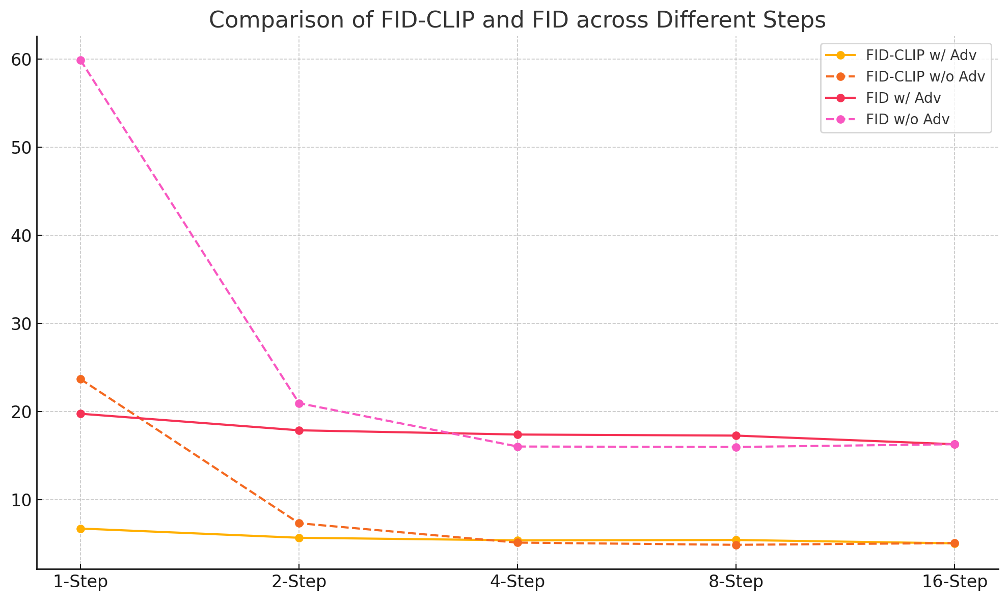
Adversarial consistency design and its effectiveness. We show the ablation study on the adversarial consistency loss design and its effectiveness. From the architecture level of discriminator, we compare the latent discriminator shared from the teacher diffusion model and the pixel discriminator from pre-trained DINO [2]. Note that DINO is trained with 224 resolutions, therefore we should resize the generation results and feed them into DINO. We find this could make the generation results fail at details as shown in the left of Fig. 9. From the adversarial loss, we compare our adversarial loss to the normal GAN loss. We find normal GAN loss causes the training to be unstable and corrupts the generation results, which aligns with our previous analysis. For its effectiveness, we compare the FID-CLIP and FID scores with the adversarial loss or without the adversarial loss under different inference steps. Fig. 8 shows that it greatly improves the FID scores in the low-step regime and gradually coverage to similar performance of our model without using the adversarial loss as the step increases.
Refer to caption
Figure 6: Sensitivity to negative prompt.
Refer to caption
Figure 7: Effectiveness of adversarial consistency loss.
Refer to caption
Figure 8: Randomness for sampling.
Refer to caption
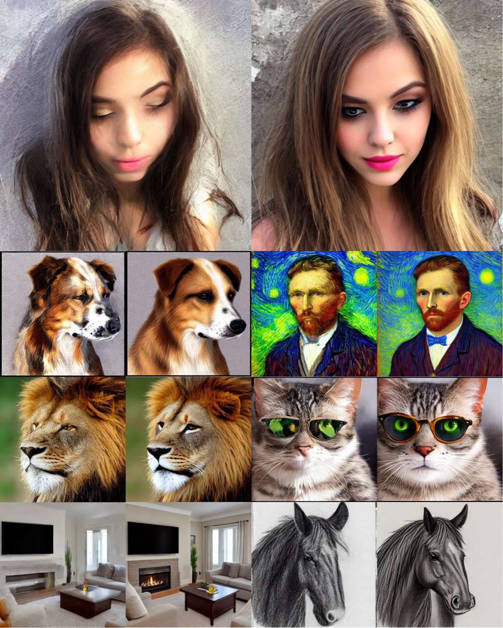
Figure 9: Ablation study on the adversarial consistency design. (Left) Replacing latent discriminator with DINO causes detail loss. (Right) Replacing our adversarial loss with normal GAN loss causes training conflicted objectives and instability.

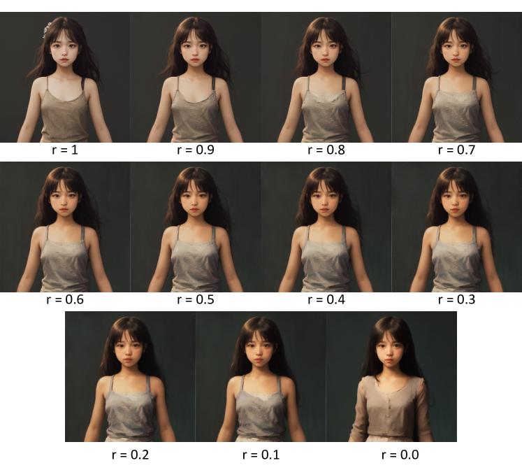
Randomness for sampling. Fig. 8 illustrates the influence of the randomness introduced in sampling as Eq. 44. The figure shows that introducing a certain of randomness in sampling may help to alleviate unrealistic objects or shapes.

5 Limitations and Conclusions

Despite being able to generate high-quality images and videos in a few steps, we find that when the number of steps is very low, especially with only one step, the generation quality is unstable. The model may produce structural errors or blurry images. Fortunately, we discover that this phenomenon can be mitigated through multi-step refinement. In conclusion, in this paper, we observe the defects in high-resolution latent space generation under text-conditional control using the consistency model. We summarize these defects on three levels, analyze their causes, and generalize its design framework to address these defects.

References

  • [1] Max Bain, Arsha Nagrani, Gül Varol, and Andrew Zisserman. Frozen in time: A joint video and image encoder for end-to-end retrieval. In ICCV, pages 1728–1738, 2021.
  • [2] Mathilde Caron, Hugo Touvron, Ishan Misra, Hervé Jégou, Julien Mairal, Piotr Bojanowski, and Armand Joulin. Emerging properties in self-supervised vision transformers. In ICCV, 2021.
  • [3] Soravit Changpinyo, Piyush Sharma, Nan Ding, and Radu Soricut. Conceptual 12m: Pushing web-scale image-text pre-training to recognize long-tail visual concepts. In CVPR, pages 3558–3568, 2021.
  • [4] Ricky TQ Chen and Yaron Lipman. Riemannian flow matching on general geometries. arXiv preprint arXiv:2302.03660, 2023.
  • [5] Prafulla Dhariwal and Alexander Nichol. Diffusion models beat gans on image synthesis. NeurIPS, 34:8780–8794, 2021.
  • [6] Patrick Esser, Sumith Kulal, Andreas Blattmann, Rahim Entezari, Jonas Müller, Harry Saini, Yam Levi, Dominik Lorenz, Axel Sauer, Frederic Boesel, et al. Scaling rectified flow transformers for high-resolution image synthesis. arXiv preprint arXiv:2403.03206, 2024.
  • [7] Jonathan Heek, Emiel Hoogeboom, and Tim Salimans. Multistep consistency models. arXiv preprint arXiv:2403.06807, 2024.
  • [8] Martin Heusel, Hubert Ramsauer, Thomas Unterthiner, Bernhard Nessler, and Sepp Hochreiter. Gans trained by a two time-scale update rule converge to a local nash equilibrium. Advances in neural information processing systems, 30, 2017.
  • [9] Jonathan Ho, Ajay Jain, and Pieter Abbeel. ddpm. NeurIPS, 33:6840–6851, 2020.
  • [10] Jonathan Ho and Tim Salimans. cfg. arXiv preprint arXiv:2207.12598, 2022.
  • [11] Tero Karras, Miika Aittala, Timo Aila, and Samuli Laine. edm. NeurIPS, 35:26565–26577, 2022.
  • [12] Dongjun Kim, Chieh-Hsin Lai, Wei-Hsiang Liao, Naoki Murata, Yuhta Takida, Toshimitsu Uesaka, Yutong He, Yuki Mitsufuji, and Stefano Ermon. Consistency trajectory models: Learning probability flow ode trajectory of diffusion. arXiv preprint arXiv:2310.02279, 2023.
  • [13] Diederik P Kingma, Tim Salimans, Ben Poole, and Jonathan Ho. On density estimation with diffusion models. In A. Beygelzimer, Y. Dauphin, P. Liang, and J. Wortman Vaughan, editors, NeurIPS, 2021.
  • [14] Fei Kong, Jinhao Duan, Lichao Sun, Hao Cheng, Renjing Xu, Hengtao Shen, Xiaofeng Zhu, Xiaoshuang Shi, and Kaidi Xu. Act-diffusion: Efficient adversarial consistency training for one-step diffusion models, 2024.
  • [15] Siqi Kou, Lanxiang Hu, Zhezhi He, Zhijie Deng, and Hao Zhang. Cllms: Consistency large language models, 2024.
  • [16] Shanchuan Lin, Anran Wang, and Xiao Yang. Sdxl-lightning: Progressive adversarial diffusion distillation. arXiv preprint arXiv:2402.13929, 2024.
  • [17] Tsung-Yi Lin, Michael Maire, Serge J. Belongie, James Hays, Pietro Perona, Deva Ramanan, Piotr Dollár, and C. Lawrence Zitnick. Microsoft COCO: common objects in context. In ECCV, volume 8693, pages 740–755. Springer, 2014.
  • [18] Yaron Lipman, Ricky TQ Chen, Heli Ben-Hamu, Maximilian Nickel, and Matt Le. Flow matching for generative modeling. arXiv preprint arXiv:2210.02747, 2022.
  • [19] Xingchao Liu, Xiwen Zhang, Jianzhu Ma, Jian Peng, et al. Instaflow: One step is enough for high-quality diffusion-based text-to-image generation. In ICLR, 2023.
  • [20] Cheng Lu, Yuhao Zhou, Fan Bao, Jianfei Chen, Chongxuan Li, and Jun Zhu. Dpm-solver: A fast ode solver for diffusion probabilistic model sampling in around 10 steps. NeurIPS, 35:5775–5787, 2022.
  • [21] Simian Luo, Yiqin Tan, Longbo Huang, Jian Li, and Hang Zhao. Latent consistency models: Synthesizing high-resolution images with few-step inference. arXiv preprint arXiv:2310.04378, 2023.
  • [22] Chenlin Meng, Robin Rombach, Ruiqi Gao, Diederik Kingma, Stefano Ermon, Jonathan Ho, and Tim Salimans. On distillation of guided diffusion models. In CVPR, pages 14297–14306, 2023.
  • [23] William Peebles and Saining Xie. Scalable diffusion models with transformers. In Proceedings of the IEEE/CVF International Conference on Computer Vision (ICCV), pages 4195–4205, October 2023.
  • [24] Dustin Podell, Zion English, Kyle Lacey, Andreas Blattmann, Tim Dockhorn, Jonas Müller, Joe Penna, and Robin Rombach. Sdxl: Improving latent diffusion models for high-resolution image synthesis. arXiv preprint arXiv:2307.01952, 2023.
  • [25] Aaditya Prasad, Kevin Lin, Jimmy Wu, Linqi Zhou, and Jeannette Bohg. Consistency policy: Accelerated visuomotor policies via consistency distillation, 2024.
  • [26] Alec Radford, Jong Wook Kim, Chris Hallacy, Aditya Ramesh, Gabriel Goh, Sandhini Agarwal, Girish Sastry, Amanda Askell, Pamela Mishkin, Jack Clark, et al. Learning transferable visual models from natural language supervision. In ICLR, pages 8748–8763. PMLR, 2021.
  • [27] Robin Rombach, Andreas Blattmann, Dominik Lorenz, Patrick Esser, and Björn Ommer. High-resolution image synthesis with latent diffusion models. In CVPR, pages 10684–10695, 2022.
  • [28] Tim Salimans and Jonathan Ho. Progressive distillation for fast sampling of diffusion models. arXiv preprint arXiv:2202.00512, 2022.
  • [29] Axel Sauer, Kashyap Chitta, Jens Müller, and Andreas Geiger. Projected gans converge faster. NeurIPS, 34:17480–17492, 2021.
  • [30] Axel Sauer, Tero Karras, Samuli Laine, Andreas Geiger, and Timo Aila. Stylegan-t: Unlocking the power of gans for fast large-scale text-to-image synthesis. In ICLR, pages 30105–30118. PMLR, 2023.
  • [31] Axel Sauer, Dominik Lorenz, Andreas Blattmann, and Robin Rombach. Adversarial diffusion distillation. arXiv preprint arXiv:2311.17042, 2023.
  • [32] Xiaoyu Shi, Zhaoyang Huang, Fu-Yun Wang, Weikang Bian, Dasong Li, Yi Zhang, Manyuan Zhang, Ka Chun Cheung, Simon See, Hongwei Qin, et al. Motion-i2v: Consistent and controllable image-to-video generation with explicit motion modeling. arXiv preprint arXiv:2401.15977, 2024.
  • [33] Jiaming Song, Chenlin Meng, and Stefano Ermon. Denoising diffusion implicit models. arXiv preprint arXiv:2010.02502, 2020.
  • [34] Yang Song and Prafulla Dhariwal. Improved techniques for training consistency models. arXiv preprint arXiv:2310.14189, 2023.
  • [35] Yang Song, Prafulla Dhariwal, Mark Chen, and Ilya Sutskever. Consistency models. arXiv preprint arXiv:2303.01469, 2023.
  • [36] Yang Song, Jascha Sohl-Dickstein, Diederik P Kingma, Abhishek Kumar, Stefano Ermon, and Ben Poole. Score-based generative modeling through stochastic differential equations. arXiv preprint arXiv:2011.13456, 2020.
  • [37] Khurram Soomro, Amir Roshan Zamir, and Mubarak Shah. UCF101: A dataset of 101 human actions classes from videos in the wild. CoRR, abs/1212.0402, 2012.
  • [38] Zachary Teed and Jia Deng. Raft: Recurrent all-pairs field transforms for optical flow, 2020.
  • [39] Fu-Yun Wang, Zhaoyang Huang, Xiaoyu Shi, Weikang Bian, Guanglu Song, Yu Liu, and Hongsheng Li. Animatelcm: Accelerating the animation of personalized diffusion models and adapters with decoupled consistency learning. arXiv preprint arXiv:2402.00769, 2024.
  • [40] Yilun Xu, Mingyang Deng, Xiang Cheng, Yonglong Tian, Ziming Liu, and Tommi Jaakkola. Restart sampling for improving generative processes, 2023.
  • [41] Yilun Xu, Shangyuan Tong, and Tommi Jaakkola. Stable target field for reduced variance score estimation in diffusion models. arXiv preprint arXiv:2302.00670, 2023.
  • [42] Richard Zhang, Phillip Isola, Alexei A. Efros, Eli Shechtman, and Oliver Wang. The unreasonable effectiveness of deep features as a perceptual metric. In CVPR, June 2018.

Appendix

\startcontents

[appendices] \printcontents[appendices]l1

Appendix I Related Works

I.1 Diffusion Models

Diffusion models [9, 36, 11] have gradually become the dominant foundation models in image synthesis. Many works have greatly explored the nature of diffusion models [18, 4, 36, 13] and generalize/improve the design space of diffusion models [33, 11, 13]. Some works explore the model architecture for diffusion models [5, 23]. Some works scale up the diffusion models for text-conditioned image synthesis or real-world applications [32, 27, 24]. Some works explore the sampling acceleration methods, including scheduler-level [11, 20, 33] or training-level [22, 35]. The formal ones are basically to explore better approximation of the PF-ODE [20, 33]. The latter are mainly distillation methods [22, 28] or initializing diffusion weights for GAN training [31, 16].

I.2 Consistency Models

The consistency model is a new family of generative models [35, 34]. It can be trained either by distillation or training without teacher models. Improved techniques even allow consistency training excelling the performance of diffusion training [34]. Consistency trajectory model (CTM) [12] innovatively proposes to learn the trajectory consistency, providing a more flexible framework. ACT combines consistency training with GAN [14] for better training efficiency. Some works apply the idea of consistency model to language model [15] and policy learning [25].

We notice that a recent work multistep consistency models [7] also proposes to splitting the ODE trajectory into multi-parts for consistency learning, and here we hope to credit their work for the valuable exploration. However, our work is principally different from multistep consistency models. Since they do not open-source their code and weights, we clarify the difference between our work and multistep consistency models based on the details of their technical report. Firstly, they didn’t provide explicit model definitions and boundary conditions nor theoretically show the error bound to prove the soundness of their work. Yet in our work, we believe we have given an explicit definition of important components and theoretically shown the soundness of each technique applied in our work. For example, they claimed using DDIM for training and inference, while in our work, we have shown that although we can also optionally parameterize as the DDIM format, there’s an intrinsic difference between that parameterization and DDIM (i.e., the difference between exact solution learning and first-order approximation). The aDDIM and invDDIM as highlighted in their pseudo code have no relation to PCM. Secondly, they are mainly for the unconditional or class-conditional generation, yet we aim for text-conditional generation in large models and dive into the influence of classifier-free guidance in consistency distillation. Besides, we innovatively introduce an adversarial loss that aligns well with consistency learning and significantly improves the generation results. We also propose simple yet effective inference techniques to enhance the generation quality and diversity for text-conditioned consistency models. We recommend readers to read their work for better comparison.

Appendix II Proofs

II.1 Phased Consistency Distillation

The following is an extension of the original proof of consistency distillation for phased consistency distillation.

Theorem 1.

For arbitrary sub-trajectory [sm,sm+1]subscript𝑠𝑚subscript𝑠𝑚1\left[s_{m},s_{m+1}\right]. let Δtm:=maxtn,tn+1[sm,sm+1]{|tn+1tn|}assignΔsubscript𝑡𝑚subscriptsubscript𝑡𝑛subscript𝑡𝑛1subscript𝑠𝑚subscript𝑠𝑚1subscript𝑡𝑛1subscript𝑡𝑛\Delta t_{m}:=\max_{t_{n},t_{n+1}\in[s_{m},s_{m+1}]}\{|t_{n+1}-t_{n}|\}, and 𝐟m(,;ϕ)superscript𝐟𝑚bold-ϕ\bm{f}^{m}(\cdot,\cdot;\bm{\phi}) be the target phased consistency function induced by the pre-trained diffusion model (empirical PF-ODE). Assume the 𝐟𝛉msubscriptsuperscript𝐟𝑚𝛉\bm{f}^{m}_{\bm{\theta}} is L𝐿L-Lipschitz and the ODE solver has local error uniformly bounded by 𝒪((tn+1tn)p+1)𝒪superscriptsubscript𝑡𝑛1subscript𝑡𝑛𝑝1\mathcal{O}((t_{n+1}-t_{n})^{p+1}) with p1𝑝1p\geq 1. Then, if PCM(𝛉,𝛉;ϕ)=0subscriptPCM𝛉𝛉bold-ϕ0\mathcal{L}_{\text{PCM}}(\bm{\theta},\bm{\theta};\bm{\phi})=0, we have

suptn,tn+1[sm,sm+1],𝐱𝒇𝜽m(𝐱,tn)𝒇m(𝐱,tn)=𝒪((Δtm)p).subscriptsupremumformulae-sequencesubscript𝑡𝑛subscript𝑡𝑛1subscript𝑠𝑚subscript𝑠𝑚1𝐱normsubscriptsuperscript𝒇𝑚𝜽𝐱subscript𝑡𝑛superscript𝒇𝑚𝐱subscript𝑡𝑛𝒪superscriptΔsubscript𝑡𝑚𝑝\displaystyle\sup_{t_{n},t_{n+1}\in[s_{m},s_{m+1}],\mathbf{x}}{\|\bm{f}^{m}_{\bm{\theta}}(\mathbf{x},t_{n})-\bm{f}^{m}(\mathbf{x},t_{n})\|}=\mathcal{O}((\Delta t_{m})^{p}).
Proof.

From the condition PCM(𝜽,𝜽;ϕ)=0subscriptPCM𝜽𝜽bold-italic-ϕ0\mathcal{L}_{\text{PCM}}(\bm{\theta},\bm{\theta};\bm{\phi})=0, for any 𝐱tnsubscript𝐱subscript𝑡𝑛\mathbf{x}_{t_{n}} and tn,tn+1[sm,sm+1]subscript𝑡𝑛subscript𝑡𝑛1subscript𝑠𝑚subscript𝑠𝑚1t_{n},t_{n+1}\in[s_{m},s_{m+1}], we have

𝒇𝜽m(𝐱tn+1,tn+1)𝒇𝜽m(𝒙^tnϕ,tn)subscriptsuperscript𝒇𝑚𝜽subscript𝐱subscript𝑡𝑛1subscript𝑡𝑛1subscriptsuperscript𝒇𝑚𝜽superscriptsubscript^𝒙subscript𝑡𝑛bold-italic-ϕsubscript𝑡𝑛\displaystyle\bm{f}^{m}_{\bm{\theta}}(\mathbf{x}_{t_{n+1},t_{n+1}})\equiv\bm{f}^{m}_{\bm{\theta}}(\hat{\bm{x}}_{t_{n}}^{\bm{\phi}},t_{n}) (10)

Denote 𝒆nm:=𝒇𝜽m(𝐱tn,tn)𝒇m(𝐱tn,tn;ϕ)assignsubscriptsuperscript𝒆𝑚𝑛subscriptsuperscript𝒇𝑚𝜽subscript𝐱subscript𝑡𝑛subscript𝑡𝑛superscript𝒇𝑚subscript𝐱subscript𝑡𝑛subscript𝑡𝑛bold-italic-ϕ\bm{e}^{m}_{n}:=\bm{f}^{m}_{\bm{\theta}}(\mathbf{x}_{t_{n}},t_{n})-\bm{f}^{m}(\mathbf{x}_{t_{n}},t_{n};\bm{\phi}), we have

𝒆n+1m=𝒇𝜽m(𝐱tn+1,tn+1)𝒇m(𝐱tn+1,tn+1;ϕ)=𝒇𝜽m(𝐱^tnϕ,tn)𝒇m(𝐱tn,tn;ϕ)=𝒇𝜽m(𝐱^tnϕ,tn)𝒇𝜽m(𝐱tn,tn)+𝒇𝜽m(𝐱tn,tn)𝒇m(𝐱tn,tn;ϕ)=𝒇𝜽m(𝐱^tnϕ,tn)𝒇𝜽m(𝐱tn,tn)+𝒆nm.subscriptsuperscript𝒆𝑚𝑛1subscriptsuperscript𝒇𝑚𝜽subscript𝐱subscript𝑡𝑛1subscript𝑡𝑛1superscript𝒇𝑚subscript𝐱subscript𝑡𝑛1subscript𝑡𝑛1bold-italic-ϕsubscriptsuperscript𝒇𝑚𝜽superscriptsubscript^𝐱subscript𝑡𝑛bold-italic-ϕsubscript𝑡𝑛superscript𝒇𝑚subscript𝐱subscript𝑡𝑛subscript𝑡𝑛bold-italic-ϕsubscriptsuperscript𝒇𝑚𝜽superscriptsubscript^𝐱subscript𝑡𝑛bold-italic-ϕsubscript𝑡𝑛subscriptsuperscript𝒇𝑚𝜽subscript𝐱subscript𝑡𝑛subscript𝑡𝑛subscriptsuperscript𝒇𝑚𝜽subscript𝐱subscript𝑡𝑛subscript𝑡𝑛superscript𝒇𝑚subscript𝐱subscript𝑡𝑛subscript𝑡𝑛bold-italic-ϕsubscriptsuperscript𝒇𝑚𝜽superscriptsubscript^𝐱subscript𝑡𝑛bold-italic-ϕsubscript𝑡𝑛subscriptsuperscript𝒇𝑚𝜽subscript𝐱subscript𝑡𝑛subscript𝑡𝑛subscriptsuperscript𝒆𝑚𝑛\begin{split}\bm{e}^{m}_{n+1}&=\bm{f}^{m}_{\bm{\theta}}(\mathbf{x}_{t_{n+1}},t_{n+1})-\bm{f}^{m}(\mathbf{x}_{t_{n+1}},t_{n+1};\bm{\phi})\\ &=\bm{f}^{m}_{\bm{\theta}}(\hat{\mathbf{x}}_{t_{n}}^{\bm{\phi}},t_{n})-\bm{f}^{m}(\mathbf{x}_{t_{n}},t_{n};\bm{\phi})\\ &=\bm{f}^{m}_{\bm{\theta}}(\hat{\mathbf{x}}_{t_{n}}^{\bm{\phi}},t_{n})-\bm{f}^{m}_{\bm{\theta}}(\mathbf{x}_{t_{n}},t_{n})+\bm{f}^{m}_{\bm{\theta}}(\mathbf{x}_{t_{n}},t_{n})-\bm{f}^{m}(\mathbf{x}_{t_{n}},t_{n};\bm{\phi})\\ &=\bm{f}^{m}_{\bm{\theta}}(\hat{\mathbf{x}}_{t_{n}}^{\bm{\phi}},t_{n})-\bm{f}^{m}_{\bm{\theta}}(\mathbf{x}_{t_{n}},t_{n})+\bm{e}^{m}_{n}\,.\end{split} (11)

Considering that 𝒇𝜽msubscriptsuperscript𝒇𝑚𝜽\bm{f}^{m}_{\bm{\theta}} is L𝐿L-Lipschitz, we have

𝒆n+1m2=𝒆nm+𝒇𝜽m(𝐱^tnϕ,tn)𝒇𝜽m(𝐱tn,tn)2𝒆nm2+𝒇𝜽m(𝐱^tnϕ,tn)𝒇𝜽m(𝐱tn,tn)2𝒆nm2+L𝐱tn𝐱tnϕ2=𝒆nm2+L𝒪((tn+1tn)p+1)𝒆nm2+L(tn+1tn)𝒪((Δtm)p).subscriptdelimited-∥∥subscriptsuperscript𝒆𝑚𝑛12subscriptdelimited-∥∥subscriptsuperscript𝒆𝑚𝑛subscriptsuperscript𝒇𝑚𝜽superscriptsubscript^𝐱subscript𝑡𝑛bold-italic-ϕsubscript𝑡𝑛subscriptsuperscript𝒇𝑚𝜽subscript𝐱subscript𝑡𝑛subscript𝑡𝑛2subscriptdelimited-∥∥subscriptsuperscript𝒆𝑚𝑛2subscriptdelimited-∥∥subscriptsuperscript𝒇𝑚𝜽superscriptsubscript^𝐱subscript𝑡𝑛bold-italic-ϕsubscript𝑡𝑛subscriptsuperscript𝒇𝑚𝜽subscript𝐱subscript𝑡𝑛subscript𝑡𝑛2subscriptdelimited-∥∥subscriptsuperscript𝒆𝑚𝑛2𝐿subscriptdelimited-∥∥subscript𝐱subscript𝑡𝑛superscriptsubscript𝐱subscript𝑡𝑛bold-italic-ϕ2subscriptdelimited-∥∥subscriptsuperscript𝒆𝑚𝑛2𝐿𝒪superscriptsubscript𝑡𝑛1subscript𝑡𝑛𝑝1subscriptdelimited-∥∥subscriptsuperscript𝒆𝑚𝑛2𝐿subscript𝑡𝑛1subscript𝑡𝑛𝒪superscriptΔsubscript𝑡𝑚𝑝\begin{split}\|\bm{e}^{m}_{n+1}\|_{2}&=\|\bm{e}^{m}_{n}+\bm{f}^{m}_{\bm{\theta}}(\hat{\mathbf{x}}_{t_{n}}^{\bm{\phi}},t_{n})-\bm{f}^{m}_{\bm{\theta}}(\mathbf{x}_{t_{n}},t_{n})\|_{2}\\ &\leq\|\bm{e}^{m}_{n}\|_{2}+\|\bm{f}^{m}_{\bm{\theta}}(\hat{\mathbf{x}}_{t_{n}}^{\bm{\phi}},t_{n})-\bm{f}^{m}_{\bm{\theta}}(\mathbf{x}_{t_{n}},t_{n})\|_{2}\\ &\leq\|\bm{e}^{m}_{n}\|_{2}+L\|\mathbf{x}_{t_{n}}-\mathbf{x}_{t_{n}}^{\bm{\phi}}\|_{2}\\ &=\|\bm{e}^{m}_{n}\|_{2}+L\cdot\mathcal{O}((t_{n+1}-t_{n})^{p+1})\\ &\leq\|\bm{e}^{m}_{n}\|_{2}+L(t_{n+1}-t_{n})\cdot\mathcal{O}((\Delta t_{m})^{p})\,.\end{split} (12)

Besides, due to the boundary condition, we have

𝒆smm=𝒇𝜽m(𝐱sm,sm)𝒇m(𝐱sm,sm;ϕ)=𝐱sm𝐱sm=0.superscriptsubscript𝒆subscript𝑠𝑚𝑚subscriptsuperscript𝒇𝑚𝜽subscript𝐱subscript𝑠𝑚subscript𝑠𝑚superscript𝒇𝑚subscript𝐱subscript𝑠𝑚subscript𝑠𝑚bold-italic-ϕsubscript𝐱subscript𝑠𝑚subscript𝐱subscript𝑠𝑚0\begin{split}\bm{e}_{s_{m}}^{m}&=\bm{f}^{m}_{\bm{\theta}}(\mathbf{x}_{s_{m}},s_{m})-\bm{f}^{m}(\mathbf{x}_{s_{m}},s_{m};\bm{\phi})\\ &=\mathbf{x}_{s_{m}}-\mathbf{x}_{s_{m}}\\ &=0\end{split}\,. (13)

Hence, we have

𝒆n+1m2𝒆smm2+L𝒪((Δt)p)ti,ti+1[sm,sm+1]ti+1ti=0+L𝒪((Δt)p)(sm+1sm)=𝒪((Δtm)p)subscriptdelimited-∥∥subscriptsuperscript𝒆𝑚𝑛12subscriptdelimited-∥∥subscriptsuperscript𝒆𝑚subscript𝑠𝑚2𝐿𝒪superscriptΔ𝑡𝑝subscriptsubscript𝑡𝑖subscript𝑡𝑖1subscript𝑠𝑚subscript𝑠𝑚1subscript𝑡𝑖1subscript𝑡𝑖0𝐿𝒪superscriptΔ𝑡𝑝subscript𝑠𝑚1subscript𝑠𝑚𝒪superscriptΔsubscript𝑡𝑚𝑝\begin{split}\|\bm{e}^{m}_{n+1}\|_{2}&\leq\|\bm{e}^{m}_{s_{m}}\|_{2}+L\cdot\mathcal{O}((\Delta t)^{p})\sum_{t_{i},t_{i+1}\in[s_{m},s_{m+1}]}t_{i+1}-t_{i}\\ &=0+L\cdot\mathcal{O}((\Delta t)^{p})\cdot(s_{m+1}-s_{m})\\ &=\mathcal{O}((\Delta t_{m})^{p})\end{split} (14)

Theorem 2.

For arbitrary set of sub-trajectories {[si,si+1]}i=mmsuperscriptsubscriptsubscript𝑠𝑖subscript𝑠𝑖1𝑖𝑚superscript𝑚\{\left[s_{i},s_{i+1}\right]\}_{i=m}^{m^{\prime}}. Let Δtm:=maxtn,tn+1[sm,sm+1]{|tn+1tn|}assignΔsubscript𝑡𝑚subscriptsubscript𝑡𝑛subscript𝑡𝑛1subscript𝑠𝑚subscript𝑠𝑚1subscript𝑡𝑛1subscript𝑡𝑛\Delta t_{m}:=\max_{t_{n},t_{n+1}\in[s_{m},s_{m+1}]}\{|t_{n+1}-t_{n}|\}, Δtm,m:=maxi[m,m]{Δti}assignΔsubscript𝑡𝑚superscript𝑚subscript𝑖superscript𝑚𝑚Δsubscript𝑡𝑖\Delta t_{m,m^{\prime}}:=\max_{i\in[m^{\prime},m]}\{\Delta t_{i}\}, and 𝐟m,m(,;ϕ)superscript𝐟𝑚superscript𝑚bold-ϕ\bm{f}^{m,m^{\prime}}(\cdot,\cdot;\bm{\phi}) be the target phased consistency function induced by the pre-trained diffusion model (empirical PF-ODE). Assume the 𝐟𝛉m,msubscriptsuperscript𝐟𝑚superscript𝑚𝛉\bm{f}^{m,m^{\prime}}_{\bm{\theta}} is L𝐿L-Lipschitz and the ODE solver has local error uniformly bounded by 𝒪((tn+1tn)p+1)𝒪superscriptsubscript𝑡𝑛1subscript𝑡𝑛𝑝1\mathcal{O}((t_{n+1}-t_{n})^{p+1}) with p1𝑝1p\geq 1. Then, if PCM(𝛉,𝛉;ϕ)=0subscriptPCM𝛉𝛉bold-ϕ0\mathcal{L}_{\text{PCM}}(\bm{\theta},\bm{\theta};\bm{\phi})=0, we have

suptn[sm,sm+1),𝐱𝒇𝜽m,m(𝐱,tn)𝒇m,m(𝐱,tn)=𝒪((Δtm,m)p).subscriptsupremumsubscript𝑡𝑛subscript𝑠𝑚subscript𝑠𝑚1𝐱normsubscriptsuperscript𝒇𝑚superscript𝑚𝜽𝐱subscript𝑡𝑛superscript𝒇𝑚superscript𝑚𝐱subscript𝑡𝑛𝒪superscriptΔsubscript𝑡𝑚superscript𝑚𝑝\displaystyle\sup_{t_{n}\in[s_{m},s_{m+1}),\mathbf{x}}{\|\bm{f}^{m,m^{\prime}}_{\bm{\theta}}(\mathbf{x},t_{n})-\bm{f}^{m,m^{\prime}}(\mathbf{x},t_{n})\|}=\mathcal{O}((\Delta t_{m,m^{\prime}})^{p}).
Proof.

From the condition PCM(𝜽,𝜽;ϕ)=0subscriptPCM𝜽𝜽bold-italic-ϕ0\mathcal{L}_{\text{PCM}}(\bm{\theta},\bm{\theta};\bm{\phi})=0, for any 𝐱tnsubscript𝐱subscript𝑡𝑛\mathbf{x}_{t_{n}} and tn,tn+1[sm,sm+1]subscript𝑡𝑛subscript𝑡𝑛1subscript𝑠𝑚subscript𝑠𝑚1t_{n},t_{n+1}\in[s_{m},s_{m+1}], we have

𝒇𝜽m(𝐱tn+1,tn+1)𝒇𝜽m(𝒙^tnϕ,tn)subscriptsuperscript𝒇𝑚𝜽subscript𝐱subscript𝑡𝑛1subscript𝑡𝑛1subscriptsuperscript𝒇𝑚𝜽superscriptsubscript^𝒙subscript𝑡𝑛bold-italic-ϕsubscript𝑡𝑛\displaystyle\bm{f}^{m}_{\bm{\theta}}(\mathbf{x}_{t_{n+1},t_{n+1}})\equiv\bm{f}^{m}_{\bm{\theta}}(\hat{\bm{x}}_{t_{n}}^{\bm{\phi}},t_{n}) (15)

Denote 𝒆nm,m:=𝒇𝜽m,m(𝐱tn,tn)𝒇m,m(𝐱tn,tn;ϕ)assignsubscriptsuperscript𝒆𝑚superscript𝑚𝑛subscriptsuperscript𝒇𝑚superscript𝑚𝜽subscript𝐱subscript𝑡𝑛subscript𝑡𝑛superscript𝒇𝑚superscript𝑚subscript𝐱subscript𝑡𝑛subscript𝑡𝑛bold-italic-ϕ\bm{e}^{m,m^{\prime}}_{n}:=\bm{f}^{m,m^{\prime}}_{\bm{\theta}}(\mathbf{x}_{t_{n}},t_{n})-\bm{f}^{m,m^{\prime}}(\mathbf{x}_{t_{n}},t_{n};\bm{\phi}), we have

𝒆n+1m,m=𝒇𝜽m,m(𝐱tn+1,tn+1)𝒇m,m(𝐱tn+1,tn+1;ϕ)=𝒇𝜽m,m(𝐱^tnϕ,tn)𝒇m,m(𝐱tn,tn;ϕ)=𝒇𝜽m,m(𝐱^tnϕ,tn)𝒇𝜽m,m(𝐱tn,tn)+𝒇𝜽m,m(𝐱tn,tn)𝒇m,m(𝐱tn,tn;ϕ)=𝒇𝜽m,m(𝐱^tnϕ,tn)𝒇𝜽m,m(𝐱tn,tn)+𝒆nm,m.subscriptsuperscript𝒆𝑚superscript𝑚𝑛1subscriptsuperscript𝒇𝑚superscript𝑚𝜽subscript𝐱subscript𝑡𝑛1subscript𝑡𝑛1superscript𝒇𝑚superscript𝑚subscript𝐱subscript𝑡𝑛1subscript𝑡𝑛1bold-italic-ϕsubscriptsuperscript𝒇𝑚superscript𝑚𝜽superscriptsubscript^𝐱subscript𝑡𝑛bold-italic-ϕsubscript𝑡𝑛superscript𝒇𝑚superscript𝑚subscript𝐱subscript𝑡𝑛subscript𝑡𝑛bold-italic-ϕsubscriptsuperscript𝒇𝑚superscript𝑚𝜽superscriptsubscript^𝐱subscript𝑡𝑛bold-italic-ϕsubscript𝑡𝑛subscriptsuperscript𝒇𝑚superscript𝑚𝜽subscript𝐱subscript𝑡𝑛subscript𝑡𝑛subscriptsuperscript𝒇𝑚superscript𝑚𝜽subscript𝐱subscript𝑡𝑛subscript𝑡𝑛superscript𝒇𝑚superscript𝑚subscript𝐱subscript𝑡𝑛subscript𝑡𝑛bold-italic-ϕsubscriptsuperscript𝒇𝑚superscript𝑚𝜽superscriptsubscript^𝐱subscript𝑡𝑛bold-italic-ϕsubscript𝑡𝑛subscriptsuperscript𝒇𝑚superscript𝑚𝜽subscript𝐱subscript𝑡𝑛subscript𝑡𝑛subscriptsuperscript𝒆𝑚superscript𝑚𝑛\begin{split}\bm{e}^{m,m^{\prime}}_{n+1}&=\bm{f}^{m,m^{\prime}}_{\bm{\theta}}(\mathbf{x}_{t_{n+1}},t_{n+1})-\bm{f}^{m,m^{\prime}}(\mathbf{x}_{t_{n+1}},t_{n+1};\bm{\phi})\\ &=\bm{f}^{m,m^{\prime}}_{\bm{\theta}}(\hat{\mathbf{x}}_{t_{n}}^{\bm{\phi}},t_{n})-\bm{f}^{m,m^{\prime}}(\mathbf{x}_{t_{n}},t_{n};\bm{\phi})\\ &=\bm{f}^{m,m^{\prime}}_{\bm{\theta}}(\hat{\mathbf{x}}_{t_{n}}^{\bm{\phi}},t_{n})-\bm{f}^{m,m^{\prime}}_{\bm{\theta}}(\mathbf{x}_{t_{n}},t_{n})+\bm{f}^{m,m^{\prime}}_{\bm{\theta}}(\mathbf{x}_{t_{n}},t_{n})-\bm{f}^{m,m^{\prime}}(\mathbf{x}_{t_{n}},t_{n};\bm{\phi})\\ &=\bm{f}^{m,m^{\prime}}_{\bm{\theta}}(\hat{\mathbf{x}}_{t_{n}}^{\bm{\phi}},t_{n})-\bm{f}^{m,m^{\prime}}_{\bm{\theta}}(\mathbf{x}_{t_{n}},t_{n})+\bm{e}^{m,m^{\prime}}_{n}\,.\end{split} (16)

Considering that 𝒇𝜽msubscriptsuperscript𝒇𝑚𝜽\bm{f}^{m}_{\bm{\theta}} is L𝐿L-Lipschitz, we have

𝒆n+1m,m2=𝒆nm,m+𝒇𝜽m,m(𝐱^tnϕ,tn)𝒇𝜽m,m(𝐱tn,tn)2𝒆nm,m2+𝒇𝜽m,m(𝐱^tnϕ,tn)𝒇𝜽m,m(𝐱tn,tn)2𝒆nm,m2+L𝒇𝜽m,m+1(𝐱^tnϕ,tn)𝒇𝜽m,m+1(𝐱tn,tn)2𝒆nm,m2+L2𝒇𝜽m,m+2(𝐱^tnϕ,tn)𝒇𝜽m,m+2(𝐱tn,tn)2𝒆nm,m2+Lmm𝒇𝜽m(𝐱^tnϕ,tn)𝒇𝜽m(𝐱tn,tn)2𝒆nm,m2+Lmm+1𝐱tn𝐱tnϕ2=𝒆nm,m2+Lmm+1𝒪((tn+1tn)p+1)𝒆nm,m2+Lmm+1(tn+1tn)𝒪((Δtm)p).\begin{split}\|\bm{e}^{m,m^{\prime}}_{n+1}\|_{2}&=\|\bm{e}^{m,m^{\prime}}_{n}+\bm{f}^{m,m^{\prime}}_{\bm{\theta}}(\hat{\mathbf{x}}_{t_{n}}^{\bm{\phi}},t_{n})-\bm{f}^{m,m^{\prime}}_{\bm{\theta}}(\mathbf{x}_{t_{n}},t_{n})\|_{2}\\ &\leq\|\bm{e}^{m,m^{\prime}}_{n}\|_{2}+\|\bm{f}^{m,m^{\prime}}_{\bm{\theta}}(\hat{\mathbf{x}}_{t_{n}}^{\bm{\phi}},t_{n})-\bm{f}^{m,m^{\prime}}_{\bm{\theta}}(\mathbf{x}_{t_{n}},t_{n})\|_{2}\\ &\leq\|\bm{e}^{m,m^{\prime}}_{n}\|_{2}+L\|\bm{f}^{m,m^{\prime}+1}_{\bm{\theta}}(\hat{\mathbf{x}}_{t_{n}}^{\bm{\phi}},t_{n})-\bm{f}^{m,m^{\prime}+1}_{\bm{\theta}}(\mathbf{x}_{t_{n}},t_{n})\|_{2}\\ &\leq\|\bm{e}^{m,m^{\prime}}_{n}\|_{2}+L^{2}\|\bm{f}^{m,m^{\prime}+2}_{\bm{\theta}}(\hat{\mathbf{x}}_{t_{n}}^{\bm{\phi}},t_{n})-\bm{f}^{m,m^{\prime}+2}_{\bm{\theta}}(\mathbf{x}_{t_{n}},t_{n})\|_{2}\\ &\leq\qquad\vdots\\ &\leq\|\bm{e}^{m,m^{\prime}}_{n}\|_{2}+L^{m-m^{\prime}}\|\bm{f}^{m}_{\bm{\theta}}(\hat{\mathbf{x}}_{t_{n}}^{\bm{\phi}},t_{n})-\bm{f}^{m}_{\bm{\theta}}(\mathbf{x}_{t_{n}},t_{n})\|_{2}\\ &\leq\|\bm{e}^{m,m^{\prime}}_{n}\|_{2}+L^{m-m^{\prime}+1}\|\mathbf{x}_{t_{n}}-\mathbf{x}_{t_{n}}^{\bm{\phi}}\|_{2}\\ &=\|\bm{e}^{m,m^{\prime}}_{n}\|_{2}+L^{m-m^{\prime}+1}\cdot\mathcal{O}((t_{n+1}-t_{n})^{p+1})\\ &\leq\|\bm{e}^{m,m^{\prime}}_{n}\|_{2}+L^{m-m^{\prime}+1}(t_{n+1}-t_{n})\cdot\mathcal{O}((\Delta t_{m})^{p})\,.\end{split} (17)

Hence, we have

𝒆n+1m,m2𝒆smm,m2+Lmm+1𝒪((Δt)p)ti,ti+1[sm,sm+1]ti+1ti=𝒆smm,m2+Lmm+1𝒪((Δt)p)(sm+1sm)=𝒆smm,m2+𝒪((Δtm)p)=𝒆smm1,m2+𝒪((Δtm)p),subscriptdelimited-∥∥subscriptsuperscript𝒆𝑚superscript𝑚𝑛12subscriptdelimited-∥∥superscriptsubscript𝒆subscript𝑠𝑚𝑚superscript𝑚2superscript𝐿𝑚superscript𝑚1𝒪superscriptΔ𝑡𝑝subscriptsubscript𝑡𝑖subscript𝑡𝑖1subscript𝑠𝑚subscript𝑠𝑚1subscript𝑡𝑖1subscript𝑡𝑖subscriptdelimited-∥∥subscriptsuperscript𝒆𝑚superscript𝑚subscript𝑠𝑚2superscript𝐿𝑚superscript𝑚1𝒪superscriptΔ𝑡𝑝subscript𝑠𝑚1subscript𝑠𝑚subscriptdelimited-∥∥subscriptsuperscript𝒆𝑚superscript𝑚subscript𝑠𝑚2𝒪superscriptΔsubscript𝑡𝑚𝑝subscriptdelimited-∥∥subscriptsuperscript𝒆𝑚1superscript𝑚subscript𝑠𝑚2𝒪superscriptΔsubscript𝑡𝑚𝑝\begin{split}\|\bm{e}^{m,m^{\prime}}_{n+1}\|_{2}&\leq\|\bm{e}_{s_{m}}^{m,m^{\prime}}\|_{2}+L^{m-m^{\prime}+1}\cdot\mathcal{O}((\Delta t)^{p})\sum_{t_{i},t_{i+1}\in[s_{m},s_{m+1}]}t_{i+1}-t_{i}\\ &=\|\bm{e}^{m,m^{\prime}}_{s_{m}}\|_{2}+L^{m-m^{\prime}+1}\cdot\mathcal{O}((\Delta t)^{p})\cdot(s_{m+1}-s_{m})\\ &=\|\bm{e}^{m,m^{\prime}}_{s_{m}}\|_{2}+\mathcal{O}((\Delta t_{m})^{p})\\ &=\|\bm{e}^{m-1,m^{\prime}}_{s_{m}}\|_{2}+\mathcal{O}((\Delta t_{m})^{p})\\ \end{split}\,, (18)

Where the last equation is due to the boundary condition 𝒇𝜽m,m(𝐱sm,sm)=𝒇𝜽m1,m(𝒇𝜽m(𝐱sm,sm),sm)=𝐟𝜽m1,m(𝐱sm,sm)subscriptsuperscript𝒇𝑚superscript𝑚𝜽subscript𝐱subscript𝑠𝑚subscript𝑠𝑚superscriptsubscript𝒇𝜽𝑚1superscript𝑚subscriptsuperscript𝒇𝑚𝜽subscript𝐱subscript𝑠𝑚subscript𝑠𝑚subscript𝑠𝑚superscriptsubscript𝐟𝜽𝑚1superscript𝑚subscript𝐱subscript𝑠𝑚subscript𝑠𝑚\bm{f}^{m,m^{\prime}}_{\bm{\theta}}(\mathbf{x}_{s_{m}},s_{m})=\bm{f}_{\bm{\theta}}^{m-1,m^{\prime}}(\bm{f}^{m}_{\bm{\theta}}(\mathbf{x}_{s_{m}},s_{m}),s_{m})=\mathbf{f}_{\bm{\theta}}^{m-1,m^{\prime}}(\mathbf{x}_{s_{m}},s_{m}).

Thereby, we have

𝒆n+1m,m2𝒆smm1,m2+𝒪((Δtm)p)𝒆sm1m2,m2+𝒪((Δtm)p)+𝒪((Δtm1)p)esm+1m+i=mm+1𝒪((Δti)p)i=mm𝒪((Δti)p)(mm+1)𝒪((Δtm,m)p)=𝒪((Δtm,m)p)\begin{split}\|\bm{e}^{m,m^{\prime}}_{n+1}\|_{2}&\leq\|\bm{e}^{m-1,m^{\prime}}_{s_{m}}\|_{2}+\mathcal{O}((\Delta t_{m})^{p})\\ &\leq\|\bm{e}_{s_{m-1}}^{m-2,m^{\prime}}\|_{2}+\mathcal{O}((\Delta t_{m})^{p})+\mathcal{O}((\Delta t_{m-1})^{p})\\ &\leq\qquad\vdots\\ &\leq\|e_{s_{m^{\prime}+1}}^{m^{\prime}}\|+\sum_{i=m}^{m^{\prime}+1}\mathcal{O}((\Delta t_{i})^{p})\\ &\leq\sum_{i=m}^{m^{\prime}}\mathcal{O}((\Delta t_{i})^{p})\\ &\leq(m-m^{\prime}+1)\mathcal{O}((\Delta t_{m,m^{\prime}})^{p})\\ &=\mathcal{O}((\Delta t_{m,m^{\prime}})^{p})\end{split} (19)

II.2 Parameterization Equivalence

We show that the parameterization of Equation. 3 is equal to the DDIM inference format.

Theorem 3.

Define F𝛉(𝐱t,t,s)=αsαt𝐱tαsϵ^𝛉(𝐱t,t)λtλseλdλsubscript𝐹𝛉subscript𝐱𝑡𝑡𝑠subscript𝛼𝑠subscript𝛼𝑡subscript𝐱𝑡subscript𝛼𝑠subscript^italic-ϵ𝛉subscript𝐱𝑡𝑡superscriptsubscriptsubscript𝜆𝑡subscript𝜆𝑠superscript𝑒𝜆differential-d𝜆F_{\bm{\theta}}(\mathbf{x}_{t},t,s)=\frac{\alpha_{s}}{\alpha_{t}}\mathbf{x}_{t}-\alpha_{s}\hat{\epsilon}_{\bm{\theta}}(\mathbf{x}_{t},t)\int_{\lambda_{t}}^{\lambda_{s}}e^{-\lambda}\mathrm{d}\lambda, then the parameterization has the same format of DDIM 𝐱s=αs(𝐱tσtϵ^𝛉(𝐱t,t)αt)+σsϵ^𝛉(𝐱t,t)subscript𝐱𝑠subscript𝛼𝑠subscript𝐱𝑡subscript𝜎𝑡subscript^bold-ϵ𝛉subscript𝐱𝑡𝑡subscript𝛼𝑡subscript𝜎𝑠subscript^bold-ϵ𝛉subscript𝐱𝑡𝑡\mathbf{x}_{s}=\alpha_{s}\left(\frac{\mathbf{x}_{t}-\sigma_{t}\hat{\bm{\epsilon}}_{\bm{\theta}}(\mathbf{x}_{t},t)}{\alpha_{t}}\right)+\sigma_{s}\hat{\bm{\epsilon}}_{\bm{\theta}}(\mathbf{x}_{t},t).

Proof.
F𝜽(𝐱t,t,s)=αsαt𝐱tαsϵ^𝜽(𝐱t,t)λtλseλdλ=αsαt𝐱tαs^ϵ𝜽(𝐱t,t)(eλteλs)=αsαt𝐱tαs^ϵ𝜽(𝐱t,t)(σtαtσsαs)=αsαt𝐱tαsσtαtϵ^𝜽(𝐱t,t)+σsϵ^𝜽(𝐱t,t)=αs(𝐱tσtϵ^𝜽(𝐱t,t)αt)+σsϵ^𝜽(𝐱t,t)subscript𝐹𝜽subscript𝐱𝑡𝑡𝑠subscript𝛼𝑠subscript𝛼𝑡subscript𝐱𝑡subscript𝛼𝑠subscript^italic-ϵ𝜽subscript𝐱𝑡𝑡superscriptsubscriptsubscript𝜆𝑡subscript𝜆𝑠superscript𝑒𝜆differential-d𝜆subscript𝛼𝑠subscript𝛼𝑡subscript𝐱𝑡subscript𝛼𝑠bold-^absentsubscriptitalic-ϵ𝜽subscript𝐱𝑡𝑡superscript𝑒subscript𝜆𝑡superscript𝑒subscript𝜆𝑠subscript𝛼𝑠subscript𝛼𝑡subscript𝐱𝑡subscript𝛼𝑠bold-^absentsubscriptitalic-ϵ𝜽subscript𝐱𝑡𝑡subscript𝜎𝑡subscript𝛼𝑡subscript𝜎𝑠subscript𝛼𝑠subscript𝛼𝑠subscript𝛼𝑡subscript𝐱𝑡subscript𝛼𝑠subscript𝜎𝑡subscript𝛼𝑡subscript^bold-italic-ϵ𝜽subscript𝐱𝑡𝑡subscript𝜎𝑠subscript^bold-italic-ϵ𝜽subscript𝐱𝑡𝑡subscript𝛼𝑠subscript𝐱𝑡subscript𝜎𝑡subscript^bold-italic-ϵ𝜽subscript𝐱𝑡𝑡subscript𝛼𝑡subscript𝜎𝑠subscript^bold-italic-ϵ𝜽subscript𝐱𝑡𝑡\begin{split}F_{\bm{\theta}}(\mathbf{x}_{t},t,s)&=\frac{\alpha_{s}}{\alpha_{t}}\mathbf{x}_{t}-\alpha_{s}\hat{\epsilon}_{\bm{\theta}}(\mathbf{x}_{t},t)\int_{\lambda_{t}}^{\lambda_{s}}e^{-\lambda}\mathrm{d}\lambda\\ &=\frac{\alpha_{s}}{\alpha_{t}}\mathbf{x}_{t}-\alpha_{s}\bm{\hat{}}{\epsilon}_{\bm{\theta}}(\mathbf{x}_{t},t)\left(e^{-\lambda_{t}}-e^{-\lambda_{s}}\right)\\ &=\frac{\alpha_{s}}{\alpha_{t}}\mathbf{x}_{t}-\alpha_{s}\bm{\hat{}}{\epsilon}_{\bm{\theta}}(\mathbf{x}_{t},t)(\frac{\sigma_{t}}{\alpha_{t}}-\frac{\sigma_{s}}{\alpha_{s}})\\ &=\frac{\alpha_{s}}{\alpha_{t}}\mathbf{x}_{t}-\frac{\alpha_{s}\sigma_{t}}{\alpha_{t}}\hat{\bm{\epsilon}}_{\bm{\theta}}(\mathbf{x}_{t},t)+\sigma_{s}\hat{\bm{\epsilon}}_{\bm{\theta}}(\mathbf{x}_{t},t)\\ &=\alpha_{s}\left(\frac{\mathbf{x}_{t}-\sigma_{t}\hat{\bm{\epsilon}}_{\bm{\theta}}(\mathbf{x}_{t},t)}{\alpha_{t}}\right)+\sigma_{s}\hat{\bm{\epsilon}}_{\bm{\theta}}(\mathbf{x}_{t},t)\end{split} (20)

II.3 Guided Distillation

We show the relationship of epsilon prediction of consistency models trained with guided distillation and diffusion models when considering the classifier-free guidance.

Theorem 4.

Assume the consistency model ϵ𝛉subscriptbold-ϵ𝛉\bm{\epsilon}_{\bm{\theta}} is trained by consistency distillation with the teacher diffusion model ϵϕsubscriptitalic-ϵbold-ϕ\epsilon_{\bm{\phi}}, and the ODE solver is augmented with CFG value w𝑤w and null text embedding \varnothing. Let 𝐜𝐜\bm{c} and 𝐜negsubscript𝐜neg\bm{c}_{\text{neg}} be the prompt and negative prompt applied for the inference of consistency model. Then, if the ODE solver is perfect and the PCM(𝛉,𝛉)=0subscriptPCM𝛉𝛉0\mathcal{L}_{\text{PCM}}(\bm{\theta},\bm{\theta})=0, we have

ϵ𝜽(𝐱,t,𝒄,𝒄n𝒆𝒈;w)subscriptbold-italic-ϵ𝜽𝐱𝑡𝒄subscript𝒄n𝒆𝒈superscript𝑤\displaystyle\bm{\epsilon}_{\bm{\theta}}(\mathbf{x},t,\bm{c},\bm{c_{\text{n}eg}};w^{\prime}) ww[ϵϕ(𝐱,t,𝒄)((1w1ww)ϵϕ(𝐱,t,𝒄neg)+w1wwϵϕ(𝐱,t,))]proportional-toabsent𝑤superscript𝑤delimited-[]subscriptbold-italic-ϵbold-italic-ϕ𝐱𝑡𝒄1𝑤1𝑤superscript𝑤subscriptbold-italic-ϵbold-italic-ϕ𝐱𝑡subscript𝒄n𝑒𝑔𝑤1𝑤superscript𝑤subscriptbold-italic-ϵbold-italic-ϕ𝐱𝑡\displaystyle\propto ww^{\prime}\left[\bm{\epsilon}_{\bm{\phi}}(\mathbf{x},t,\bm{c})-((1-\frac{w-1}{ww^{\prime}})\bm{\epsilon}_{\bm{\phi}}(\mathbf{x},t,\bm{c}_{\text{n}eg})+\frac{w-1}{ww^{\prime}}\bm{\epsilon}_{\bm{\phi}}(\mathbf{x},t,\varnothing))\right]
+ϵϕ(𝐱,t,𝒄neg)subscriptbold-italic-ϵbold-italic-ϕ𝐱𝑡subscript𝒄n𝑒𝑔\displaystyle+\bm{\epsilon}_{\bm{\phi}}(\mathbf{x},t,\bm{c}_{\text{n}eg})
Proof.

If the ODE solver is perfect, that means the empirical PF-ODE is exactly the PF-ODE of the training data. Then considering Theorem 1 and Theorem 2, it is apparent that the consistency model will fit the PF-ODE. To show that, considering the case in Theorem 1, we have

𝒆n+1m=𝒇𝜽m(𝐱tn+1,tn+1)𝒇m(𝐱tn+1,tn+1;ϕ)=𝒇𝜽m(𝐱^tnϕ,tn)𝒇m(𝐱tn,tn;ϕ)=𝒇𝜽m(𝐱^tnϕ,tn)𝒇𝜽m(𝐱tn,tn)+𝒇𝜽m(𝐱tn,tn)𝒇m(𝐱tn,tn;ϕ)=𝒇𝜽m(𝐱^tnϕ,tn)𝒇𝜽m(𝐱tn,tn)+𝒆nm=(i)𝒇𝜽m(𝐱tn,tn)𝒇𝜽m(𝐱tn,tn)+𝒆nm=𝒆nm==𝒆smm=0,subscriptsuperscript𝒆𝑚𝑛1subscriptsuperscript𝒇𝑚𝜽subscript𝐱subscript𝑡𝑛1subscript𝑡𝑛1superscript𝒇𝑚subscript𝐱subscript𝑡𝑛1subscript𝑡𝑛1bold-italic-ϕsubscriptsuperscript𝒇𝑚𝜽superscriptsubscript^𝐱subscript𝑡𝑛bold-italic-ϕsubscript𝑡𝑛superscript𝒇𝑚subscript𝐱subscript𝑡𝑛subscript𝑡𝑛bold-italic-ϕsubscriptsuperscript𝒇𝑚𝜽superscriptsubscript^𝐱subscript𝑡𝑛bold-italic-ϕsubscript𝑡𝑛subscriptsuperscript𝒇𝑚𝜽subscript𝐱subscript𝑡𝑛subscript𝑡𝑛subscriptsuperscript𝒇𝑚𝜽subscript𝐱subscript𝑡𝑛subscript𝑡𝑛superscript𝒇𝑚subscript𝐱subscript𝑡𝑛subscript𝑡𝑛bold-italic-ϕsubscriptsuperscript𝒇𝑚𝜽superscriptsubscript^𝐱subscript𝑡𝑛bold-italic-ϕsubscript𝑡𝑛subscriptsuperscript𝒇𝑚𝜽subscript𝐱subscript𝑡𝑛subscript𝑡𝑛subscriptsuperscript𝒆𝑚𝑛𝑖subscriptsuperscript𝒇𝑚𝜽subscript𝐱subscript𝑡𝑛subscript𝑡𝑛subscriptsuperscript𝒇𝑚𝜽subscript𝐱subscript𝑡𝑛subscript𝑡𝑛subscriptsuperscript𝒆𝑚𝑛superscriptsubscript𝒆𝑛𝑚superscriptsubscript𝒆subscript𝑠𝑚𝑚0\begin{split}\bm{e}^{m}_{n+1}&=\bm{f}^{m}_{\bm{\theta}}(\mathbf{x}_{t_{n+1}},t_{n+1})-\bm{f}^{m}(\mathbf{x}_{t_{n+1}},t_{n+1};\bm{\phi})\\ &=\bm{f}^{m}_{\bm{\theta}}(\hat{\mathbf{x}}_{t_{n}}^{\bm{\phi}},t_{n})-\bm{f}^{m}(\mathbf{x}_{t_{n}},t_{n};\bm{\phi})\\ &=\bm{f}^{m}_{\bm{\theta}}(\hat{\mathbf{x}}_{t_{n}}^{\bm{\phi}},t_{n})-\bm{f}^{m}_{\bm{\theta}}(\mathbf{x}_{t_{n}},t_{n})+\bm{f}^{m}_{\bm{\theta}}(\mathbf{x}_{t_{n}},t_{n})-\bm{f}^{m}(\mathbf{x}_{t_{n}},t_{n};\bm{\phi})\\ &=\bm{f}^{m}_{\bm{\theta}}(\hat{\mathbf{x}}_{t_{n}}^{\bm{\phi}},t_{n})-\bm{f}^{m}_{\bm{\theta}}(\mathbf{x}_{t_{n}},t_{n})+\bm{e}^{m}_{n}\\ &\overset{(i)}{=}\bm{f}^{m}_{\bm{\theta}}(\mathbf{x}_{t_{n}},t_{n})-\bm{f}^{m}_{\bm{\theta}}(\mathbf{x}_{t_{n}},t_{n})+\bm{e}^{m}_{n}\\ &=\bm{e}_{n}^{m}\\ &=\vdots\\ &=\bm{e}_{s_{m}}^{m}\\ &=0\,,\end{split} (21)

where (i)𝑖(i) is because the ODE solver is perfect. Considering our parameterization in Equation 3, then it should be equal to the exact solution in Equation 2. That is,

αsαt𝐱tαsϵ^θ(𝐱t,t)λtλseλdλ=αsαt𝐱t+αsλtλseλσtλ(λ)logtλ(λ)(𝐱tλ(λ))dλϵ^𝜽(𝐱t,t)λtλseλdλ=λtλseλϵϕ(𝐱tλ(λ),tλ(λ))dλϵ^𝜽(𝐱t,t)=λtλseλϵϕ(𝐱tλ(λ),tλ(λ))dλλtλseλdλ.subscript𝛼𝑠subscript𝛼𝑡subscript𝐱𝑡subscript𝛼𝑠subscript^bold-italic-ϵ𝜃subscript𝐱𝑡𝑡superscriptsubscriptsubscript𝜆𝑡subscript𝜆𝑠superscript𝑒𝜆differential-d𝜆subscript𝛼𝑠subscript𝛼𝑡subscript𝐱𝑡subscript𝛼𝑠superscriptsubscriptsubscript𝜆𝑡subscript𝜆𝑠superscript𝑒𝜆subscript𝜎subscript𝑡𝜆𝜆subscriptsubscript𝑡𝜆𝜆subscript𝐱subscript𝑡𝜆𝜆differential-d𝜆subscript^bold-italic-ϵ𝜽subscript𝐱𝑡𝑡superscriptsubscriptsubscript𝜆𝑡subscript𝜆𝑠superscript𝑒𝜆differential-d𝜆superscriptsubscriptsubscript𝜆𝑡subscript𝜆𝑠superscript𝑒𝜆subscriptbold-italic-ϵbold-italic-ϕsubscript𝐱subscript𝑡𝜆𝜆subscript𝑡𝜆𝜆differential-d𝜆subscript^bold-italic-ϵ𝜽subscript𝐱𝑡𝑡superscriptsubscriptsubscript𝜆𝑡subscript𝜆𝑠superscript𝑒𝜆subscriptbold-italic-ϵbold-italic-ϕsubscript𝐱subscript𝑡𝜆𝜆subscript𝑡𝜆𝜆differential-d𝜆superscriptsubscriptsubscript𝜆𝑡subscript𝜆𝑠superscript𝑒𝜆differential-d𝜆\begin{split}\frac{\alpha_{s}}{\alpha_{t}}\mathbf{x}_{t}-\alpha_{s}\hat{\bm{\epsilon}}_{\theta}({\mathbf{x}_{t},t})\int_{\lambda_{t}}^{\lambda_{s}}e^{-\lambda}\mathrm{d}\lambda&=\frac{\alpha_{s}}{\alpha_{t}}\mathbf{x}_{t}+\alpha_{s}\int_{\lambda_{t}}^{\lambda_{s}}e^{-\lambda}{\sigma_{t_{\lambda}(\lambda)}}\nabla\log\mathbb{P}_{t_{\lambda}(\lambda)}(\mathbf{x}_{t_{\lambda}(\lambda)})\mathrm{d}\lambda\\ \hat{\bm{\epsilon}}_{\bm{\theta}}({\mathbf{x}_{t},t})\int_{\lambda_{t}}^{\lambda_{s}}e^{-\lambda}\mathrm{d}\lambda&=\int_{\lambda_{t}}^{\lambda_{s}}e^{-\lambda}\bm{\epsilon}_{\bm{\phi}}(\mathbf{x}_{t_{\lambda}(\lambda)},t_{\lambda}(\lambda))\mathrm{d}\lambda\\ \hat{\bm{\epsilon}}_{\bm{\theta}}({\mathbf{x}_{t},t})&=\frac{\int_{\lambda_{t}}^{\lambda_{s}}e^{-\lambda}\bm{\epsilon}_{\bm{\phi}}(\mathbf{x}_{t_{\lambda}(\lambda)},t_{\lambda}(\lambda))\mathrm{d}\lambda}{\int_{\lambda_{t}}^{\lambda_{s}}e^{-\lambda}\mathrm{d}\lambda}\,.\end{split} (22)

Then we have the epsilon prediction is weighted integral of diffusion-based epsilon prediction on the trajectory. Therefore, it is apparent that, for any ttsuperscript𝑡𝑡t^{\prime}\leq t and tsuperscript𝑡t^{\prime} on the same sub-trajectory with t𝑡t, we have

ϵ^𝜽(𝐱t,t)ϵϕ(𝐱t,t)proportional-tosubscript^bold-italic-ϵ𝜽subscript𝐱𝑡𝑡subscriptitalic-ϵbold-italic-ϕsubscript𝐱superscript𝑡superscript𝑡\hat{\bm{\epsilon}}_{\bm{\theta}}(\mathbf{x}_{t},t)\propto\epsilon_{\bm{\phi}}(\mathbf{x}_{t^{\prime}},t^{\prime}) (23)

When considering the text-conditioned generation and the ODE solver being augmented with the CFG value w𝑤w, we have

ϵ^𝜽(𝐱t,t,𝒄)ϵϕ(𝐱t,t,)+w(ϵϕ(𝐱t,t,𝒄)ϵϕ(𝐱t,t,)).proportional-tosubscript^bold-italic-ϵ𝜽subscript𝐱𝑡𝑡𝒄subscriptbold-italic-ϵbold-italic-ϕsubscript𝐱superscript𝑡superscript𝑡𝑤subscriptbold-italic-ϵbold-italic-ϕsubscript𝐱superscript𝑡superscript𝑡𝒄subscriptbold-italic-ϵbold-italic-ϕsubscript𝐱superscript𝑡superscript𝑡\hat{\bm{\epsilon}}_{\bm{\theta}}(\mathbf{x}_{t},t,\bm{c})\propto\bm{\epsilon}_{\bm{\phi}}(\mathbf{x}_{t^{\prime}},t^{\prime},\varnothing)+w(\bm{\epsilon}_{\bm{\phi}}(\mathbf{x}_{t^{\prime}},t^{\prime},\bm{c})-\bm{\epsilon}_{\bm{\phi}}(\mathbf{x}_{t^{\prime}},t^{\prime},\varnothing))\,. (24)

If we additionally apply the classifier-free guidance to the consistency models with negative prompt embedding 𝒄negsubscript𝒄n𝑒𝑔\bm{c}_{\text{n}eg} and CFG value wsuperscript𝑤w^{\prime}, we have

ϵ^𝜽(𝐱t,t,𝒄,𝒄neg;w)=ϵ^𝜽(𝐱t,t,𝒄neg)+w(ϵ^𝜽(𝐱t,t,𝒄)ϵ^𝜽(𝐱t,t,𝒄neg))ϵϕ(𝐱t,t,)+w(ϵϕ(𝐱t,t,𝒄)ϵϕ(𝐱t,t,))+w{[ϵϕ(𝐱t,t,)+w(ϵϕ(𝐱t,t,𝒄)ϵϕ(𝐱t,t,))][ϵϕ(𝐱t,t,)+w(ϵϕ(𝐱t,t,𝒄)ϵϕ(𝐱t,t,))]}=ϵϕ(𝐱t,t,)+w(ϵϕ(𝐱t,t,𝒄neg)ϵϕ(𝐱t,t,))+ww(ϵϕ(𝐱t,t,𝒄)ϵϕ(𝐱t,t,𝒄neg))=ww(ϵϕ(𝐱,t,𝒄)((1α)ϵϕ(𝐱,t,𝒄neg)+αϵϕ(𝐱,t,)))+ϵϕ(𝐱,t,𝒄neg)subscript^bold-italic-ϵ𝜽subscript𝐱𝑡𝑡𝒄subscript𝒄n𝑒𝑔superscript𝑤subscript^bold-italic-ϵ𝜽subscript𝐱𝑡𝑡subscript𝒄n𝑒𝑔superscript𝑤subscript^bold-italic-ϵ𝜽subscript𝐱𝑡𝑡𝒄subscript^bold-italic-ϵ𝜽subscript𝐱𝑡𝑡subscript𝒄negproportional-tosubscriptbold-italic-ϵbold-italic-ϕsubscript𝐱superscript𝑡superscript𝑡𝑤subscriptbold-italic-ϵbold-italic-ϕsubscript𝐱superscript𝑡superscript𝑡𝒄subscriptbold-italic-ϵbold-italic-ϕsubscript𝐱superscript𝑡superscript𝑡superscript𝑤delimited-[]subscriptbold-italic-ϵbold-italic-ϕsubscript𝐱superscript𝑡superscript𝑡𝑤subscriptbold-italic-ϵbold-italic-ϕsubscript𝐱superscript𝑡superscript𝑡𝒄subscriptbold-italic-ϵbold-italic-ϕsubscript𝐱superscript𝑡superscript𝑡delimited-[]subscriptbold-italic-ϵbold-italic-ϕsubscript𝐱superscript𝑡superscript𝑡𝑤subscriptbold-italic-ϵbold-italic-ϕsubscript𝐱superscript𝑡superscript𝑡𝒄subscriptbold-italic-ϵbold-italic-ϕsubscript𝐱superscript𝑡superscript𝑡subscriptbold-italic-ϵbold-italic-ϕsubscript𝐱superscript𝑡superscript𝑡𝑤subscriptbold-italic-ϵbold-italic-ϕsubscript𝐱superscript𝑡superscript𝑡subscript𝒄n𝑒𝑔subscriptbold-italic-ϵbold-italic-ϕsubscript𝐱superscript𝑡superscript𝑡𝑤superscript𝑤subscriptbold-italic-ϵbold-italic-ϕsubscript𝐱superscript𝑡superscript𝑡𝒄subscriptbold-italic-ϵbold-italic-ϕsubscript𝐱superscript𝑡superscript𝑡subscript𝒄neg𝑤superscript𝑤subscriptbold-italic-ϵbold-italic-ϕ𝐱𝑡𝒄1𝛼subscriptbold-italic-ϵbold-italic-ϕ𝐱𝑡subscript𝒄neg𝛼subscriptbold-italic-ϵbold-italic-ϕ𝐱𝑡subscriptbold-italic-ϵbold-italic-ϕ𝐱𝑡subscript𝒄neg\begin{split}\hat{\bm{\epsilon}}_{\bm{\theta}}(\mathbf{x}_{t},t,\bm{c},\bm{c}_{\text{n}eg};w^{\prime})&=\hat{\bm{\epsilon}}_{\bm{\theta}}(\mathbf{x}_{t},t,\bm{c}_{\text{n}eg})+w^{\prime}(\hat{\bm{\epsilon}}_{\bm{\theta}}(\mathbf{x}_{t},t,\bm{c})-\hat{\bm{\epsilon}}_{\bm{\theta}}(\mathbf{x}_{t},t,\bm{c}_{\text{neg}}))\\ &\propto\bm{\epsilon}_{\bm{\phi}}(\mathbf{x}_{t^{\prime}},t^{\prime},\varnothing)+w(\bm{\epsilon}_{\bm{\phi}}(\mathbf{x}_{t^{\prime}},t^{\prime},\bm{c})-\bm{\epsilon}_{\bm{\phi}}(\mathbf{x}_{t^{\prime}},t^{\prime},\varnothing))\\ +w^{\prime}\{[\bm{\epsilon}_{\bm{\phi}}(\mathbf{x}_{t^{\prime}},t^{\prime},\varnothing)+&w(\bm{\epsilon}_{\bm{\phi}}(\mathbf{x}_{t^{\prime}},t^{\prime},\bm{c})-\bm{\epsilon}_{\bm{\phi}}(\mathbf{x}_{t^{\prime}},t^{\prime},\varnothing))]-[\bm{\epsilon}_{\bm{\phi}}(\mathbf{x}_{t^{\prime}},t^{\prime},\varnothing)+w(\bm{\epsilon}_{\bm{\phi}}(\mathbf{x}_{t^{\prime}},t^{\prime},\bm{c})-\bm{\epsilon}_{\bm{\phi}}(\mathbf{x}_{t^{\prime}},t^{\prime},\varnothing))]\}\\ &=\bm{\epsilon}_{\bm{\phi}}(\mathbf{x}_{t^{\prime}},t^{\prime},\varnothing)+w(\bm{\epsilon}_{\bm{\phi}}(\mathbf{x}_{t^{\prime}},t^{\prime},\bm{c}_{\text{n}eg})-\bm{\epsilon}_{\bm{\phi}}(\mathbf{x}_{t^{\prime}},t^{\prime},\varnothing))+ww^{\prime}(\bm{\epsilon}_{\bm{\phi}}(\mathbf{x}_{t^{\prime}},t^{\prime},\bm{c})-\bm{\epsilon}_{\bm{\phi}}(\mathbf{x}_{t^{\prime}},t^{\prime},\bm{c}_{\text{neg}}))\\ &=ww^{\prime}(\bm{\epsilon}_{\bm{\phi}}(\mathbf{x},t,\bm{c})-((1-\alpha)\bm{\epsilon}_{\bm{\phi}}(\mathbf{x},t,\bm{c}_{\text{neg}})+\alpha\bm{\epsilon}_{\bm{\phi}}(\mathbf{x},t,\varnothing)))+\bm{\epsilon}_{\bm{\phi}}(\mathbf{x},t,\bm{c}_{\text{neg}})\end{split} (25)

II.4 Distribution Consistency Convergence

We firstly show that when PCM=0subscriptPCM0\mathcal{L}_{\text{PCM}}=0 is achieved, our distribution consistency loss will also converge to zero. Then, we additionally show that, when considering the pre-train data distribution and distillation data distribution mismatch, combining GAN is a flawed design. The loss is still non-zero even when the self-consistency is achieved, thus corrupting the training.

Theorem 5.

Denote the data distribution applied for consistency distillation phased is 0subscript0\mathbb{P}_{0}. And considering that the forward conditional probability path is defined by αt𝐱0+σtϵsubscript𝛼𝑡subscript𝐱0subscript𝜎𝑡bold-ϵ\alpha_{t}\mathbf{x}_{0}+\sigma_{t}\bm{\epsilon}, we further define the intermediate distribution t(𝐱)=(0(𝐱αt)1αt)𝒩(0,σt)subscript𝑡𝐱subscript0𝐱subscript𝛼𝑡1subscript𝛼𝑡𝒩0subscript𝜎𝑡\mathbb{P}_{t}(\mathbf{x})=(\mathbb{P}_{0}(\frac{\mathbf{x}}{\alpha_{t}})\cdot\frac{1}{\alpha_{t}})\ast\mathcal{N}(0,\sigma_{t}). Similarly, we denote the data distribution applied for pretraining the diffusion model is 0pretrain(𝐱)subscriptsuperscriptpretrain0𝐱\mathbb{P}^{\text{pretrain}}_{0}(\mathbf{x}) and the intermediate distribution following forward process are tpretrain(𝐱)=(tpretrain(𝐱)=(0pretrain(𝐱αt)1αt)𝒩(0,σt))subscriptsuperscriptpretrain𝑡𝐱subscriptsuperscriptpretrain𝑡𝐱subscriptsuperscriptpretrain0𝐱subscript𝛼𝑡1subscript𝛼𝑡𝒩0subscript𝜎𝑡\mathbb{P}^{\text{pretrain}}_{t}(\mathbf{x})=(\mathbb{P}^{\text{pretrain}}_{t}(\mathbf{x})=(\mathbb{P}^{\text{pretrain}}_{0}(\frac{\mathbf{x}}{\alpha_{t}})\cdot\frac{1}{\alpha_{t}})\ast\mathcal{N}(0,\sigma_{t})). This is reasonable since current large diffusion models are typically trained with much more resources on much larger datasets compared to those of consistency distillation. And, we denote the flow 𝒯tsϕsubscriptsuperscript𝒯bold-ϕ𝑡𝑠\mathcal{T}^{\bm{\phi}}_{t\to s}, 𝒯ts𝛉subscriptsuperscript𝒯𝛉𝑡𝑠\mathcal{T}^{\bm{\theta}}_{t\to s}, and 𝒯tsϕsubscriptsuperscript𝒯superscriptitalic-ϕ𝑡𝑠\mathcal{T}^{\phi^{\prime}}_{t\to s} correspond to our consistency model, pre-trained diffusion model, and the PF-ODE of the data distribution used for consistency distillation, respectively. Additionally, let 𝒯stsubscriptsuperscript𝒯𝑠𝑡\mathcal{T}^{-}_{s\to t} be the distribution transition following the forward process SDE (adding noise). Then, if the PCM=0subscriptPCM0\mathcal{L}_{\text{PCM}}=0, for arbitrary sub-trajectory [sm,sm+1]subscript𝑠𝑚subscript𝑠𝑚1[s_{m},s_{m+1}], we have,

PCMadv(𝜽,𝜽;ϕ,m)=D(𝒯sms𝒯tn+1sm𝜽#tn+1𝒯sms𝒯tnsm𝜽𝒯tn+1tnϕ#tn+1)=0.\displaystyle\mathcal{L}_{\text{PCM}}^{adv}(\bm{\theta},\bm{\theta};\bm{\phi},m)=D\left(\mathcal{T}^{-}_{s_{m}\to s}\mathcal{T}^{\bm{\theta}}_{t_{n+1}\to s_{m}}\#\mathbb{P}_{t_{n+1}}\middle\|\mathcal{T}^{-}_{s_{m}\to s}\mathcal{T}^{\bm{\theta}}_{t_{n}\to s_{m}}\mathcal{T}^{\bm{\phi}}_{t_{n+1}\to t_{n}}\#\mathbb{P}_{t_{n+1}}\right)=0.
Proof.

Firstly, considering that the forward process 𝒯stsubscriptsuperscript𝒯𝑠𝑡\mathcal{T}^{-}_{s\to t} is equivalent to scaling the original variables and then performing convolution operations with 𝒩(𝟎,σst2𝐈)𝒩0superscriptsubscript𝜎𝑠𝑡2𝐈\mathcal{N}(\bm{0},\sigma_{s\to t}^{2}\mathbf{I}). Therefore, as long as

D(𝒯tn+1sm𝜽#tn+1𝒯tnsm𝜽𝒯tn+1tnϕ#tn+1)=0,D\left(\mathcal{T}^{\bm{\theta}}_{t_{n+1}\to s_{m}}\#\mathbb{P}_{t_{n+1}}\middle\|\mathcal{T}^{\bm{\theta}}_{t_{n}\to s_{m}}\mathcal{T}^{\bm{\phi}}_{t_{n+1}\to t_{n}}\#\mathbb{P}_{t_{n+1}}\right)=0\,, (26)

then we have

D(𝒯sms𝒯tn+1sm𝜽#tn+1𝒯sms𝒯tnsm𝜽𝒯tn+1tnϕ#tn+1)=0.D\left(\mathcal{T}^{-}_{s_{m}\to s}\mathcal{T}^{\bm{\theta}}_{t_{n+1}\to s_{m}}\#\mathbb{P}_{t_{n+1}}\middle\|\mathcal{T}^{-}_{s_{m}\to s}\mathcal{T}^{\bm{\theta}}_{t_{n}\to s_{m}}\mathcal{T}^{\bm{\phi}}_{t_{n+1}\to t_{n}}\#\mathbb{P}_{t_{n+1}}\right)=0\,. (27)

From the condition PCM(𝜽,𝜽;ϕ)=0subscriptPCM𝜽𝜽bold-italic-ϕ0\mathcal{L}_{\text{PCM}}(\bm{\theta},\bm{\theta};\bm{\phi})=0, for any 𝐱tntnsubscript𝐱subscript𝑡𝑛subscriptsubscript𝑡𝑛\mathbf{x}_{t_{n}}\in\mathbb{P}_{t_{n}} and 𝐱tn+1tn+1subscript𝐱subscript𝑡𝑛1subscriptsubscript𝑡𝑛1\mathbf{x}_{t_{n+1}}\in\mathbb{P}_{t_{n+1}} and tn,tn+1[sm,sm+1]subscript𝑡𝑛subscript𝑡𝑛1subscript𝑠𝑚subscript𝑠𝑚1t_{n},t_{n+1}\in[s_{m},s_{m+1}], we have

𝒇𝜽m(𝐱tn+1,tn+1)𝒇𝜽m(𝒙^tnϕ,tn),subscriptsuperscript𝒇𝑚𝜽subscript𝐱subscript𝑡𝑛1subscript𝑡𝑛1subscriptsuperscript𝒇𝑚𝜽superscriptsubscript^𝒙subscript𝑡𝑛bold-italic-ϕsubscript𝑡𝑛\displaystyle\bm{f}^{m}_{\bm{\theta}}(\mathbf{x}_{t_{n+1},t_{n+1}})\equiv\bm{f}^{m}_{\bm{\theta}}(\hat{\bm{x}}_{t_{n}}^{\bm{\phi}},t_{n})\,, (28)

which induces that

𝒯tn+1sm𝜽#tn+1𝒯tnsm𝜽𝒯tn+1tnϕ#tn+1.subscriptsuperscript𝒯𝜽subscript𝑡𝑛1subscript𝑠𝑚#subscriptsubscript𝑡𝑛1subscriptsuperscript𝒯𝜽subscript𝑡𝑛subscript𝑠𝑚subscriptsuperscript𝒯bold-italic-ϕsubscript𝑡𝑛1subscript𝑡𝑛#subscriptsubscript𝑡𝑛1\displaystyle\mathcal{T}^{\bm{\theta}}_{t_{n+1}\to s_{m}}\#\mathbb{P}_{t_{n+1}}\equiv\mathcal{T}^{\bm{\theta}}_{t_{n}\to s_{m}}\mathcal{T}^{\bm{\phi}}_{t_{n+1}\to t_{n}}\#\mathbb{P}_{t_{n+1}}\,. (29)

Therefore, we show that if PCM(𝜽,𝜽;ϕ)=0subscript𝑃𝐶𝑀𝜽𝜽bold-italic-ϕ0\mathcal{L}_{PCM}(\bm{\theta},\bm{\theta};\bm{\phi})=0, then

PCMadv(𝜽,𝜽;ϕ)=0superscriptsubscriptPCM𝑎𝑑𝑣𝜽𝜽bold-italic-ϕ0\mathcal{L}_{\text{PCM}}^{adv}(\bm{\theta},\bm{\theta};\bm{\phi})=0 (30)

Theorem 6.

Denote the data distribution applied for consistency distillation phased is 0subscript0\mathbb{P}_{0}. And considering that the forward conditional probability path is defined by αt𝐱0+σtϵsubscript𝛼𝑡subscript𝐱0subscript𝜎𝑡bold-ϵ\alpha_{t}\mathbf{x}_{0}+\sigma_{t}\bm{\epsilon}, we further define the intermediate distribution t(𝐱)=(0(𝐱αt)1αt)𝒩(0,σt)subscript𝑡𝐱subscript0𝐱subscript𝛼𝑡1subscript𝛼𝑡𝒩0subscript𝜎𝑡\mathbb{P}_{t}(\mathbf{x})=(\mathbb{P}_{0}(\frac{\mathbf{x}}{\alpha_{t}})\cdot\frac{1}{\alpha_{t}})\ast\mathcal{N}(0,\sigma_{t}). Similarly, we denote the data distribution applied for pretraining the diffusion model is 0pretrain(𝐱)subscriptsuperscriptpretrain0𝐱\mathbb{P}^{\text{pretrain}}_{0}(\mathbf{x}) and the intermediate distribution following forward process are tpretrain(𝐱)=(tpretrain(𝐱)=(0pretrain(𝐱αt)1αt)𝒩(0,σt))subscriptsuperscriptpretrain𝑡𝐱subscriptsuperscriptpretrain𝑡𝐱subscriptsuperscriptpretrain0𝐱subscript𝛼𝑡1subscript𝛼𝑡𝒩0subscript𝜎𝑡\mathbb{P}^{\text{pretrain}}_{t}(\mathbf{x})=(\mathbb{P}^{\text{pretrain}}_{t}(\mathbf{x})=(\mathbb{P}^{\text{pretrain}}_{0}(\frac{\mathbf{x}}{\alpha_{t}})\cdot\frac{1}{\alpha_{t}})\ast\mathcal{N}(0,\sigma_{t})). This is reasonable since current large diffusion models are typically trained with much more resources on much larger datasets compared to those of consistency distillation. And, we denote the flow 𝒯tsϕsubscriptsuperscript𝒯bold-ϕ𝑡𝑠\mathcal{T}^{\bm{\phi}}_{t\to s}, 𝒯ts𝛉subscriptsuperscript𝒯𝛉𝑡𝑠\mathcal{T}^{\bm{\theta}}_{t\to s}, and 𝒯tsϕsubscriptsuperscript𝒯superscriptitalic-ϕ𝑡𝑠\mathcal{T}^{\phi^{\prime}}_{t\to s} correspond to our consistency model, pre-trained diffusion model, and the PF-ODE of the data distribution used for consistency distillation, respectively. Then, if the PCM=0subscriptPCM0\mathcal{L}_{\text{PCM}}=0, for arbitrary sub-trajectory [sm,sm+1]subscript𝑠𝑚subscript𝑠𝑚1[s_{m},s_{m+1}], we have,

PCMadv(𝜽,𝜽;ϕ,m)=D(𝒯tn+1sm𝜽#tn+1sm)0.\displaystyle\mathcal{L}_{\text{PCM}}^{adv}(\bm{\theta},\bm{\theta};\bm{\phi},m)=D\left(\mathcal{T}^{\bm{\theta}}_{t_{n+1}\to s_{m}}\#\mathbb{P}_{t_{n+1}}\middle\|\mathbb{P}_{s_{m}}\right)\geq 0.
Proof.

From the condition PCM(𝜽,𝜽;ϕ)=0subscriptPCM𝜽𝜽bold-italic-ϕ0\mathcal{L}_{\text{PCM}}(\bm{\theta},\bm{\theta};\bm{\phi})=0, for any 𝐱tntnsubscript𝐱subscript𝑡𝑛subscriptsubscript𝑡𝑛\mathbf{x}_{t_{n}}\in\mathbb{P}_{t_{n}} and 𝐱tn+1tn+1subscript𝐱subscript𝑡𝑛1subscriptsubscript𝑡𝑛1\mathbf{x}_{t_{n+1}}\in\mathbb{P}_{t_{n+1}} and tn,tn+1[sm,sm+1]subscript𝑡𝑛subscript𝑡𝑛1subscript𝑠𝑚subscript𝑠𝑚1t_{n},t_{n+1}\in[s_{m},s_{m+1}], we have

𝒇𝜽m(𝐱tn+1,tn+1)𝒇𝜽m(𝒙^tnϕ,tn),subscriptsuperscript𝒇𝑚𝜽subscript𝐱subscript𝑡𝑛1subscript𝑡𝑛1subscriptsuperscript𝒇𝑚𝜽superscriptsubscript^𝒙subscript𝑡𝑛bold-italic-ϕsubscript𝑡𝑛\displaystyle\bm{f}^{m}_{\bm{\theta}}(\mathbf{x}_{t_{n+1},t_{n+1}})\equiv\bm{f}^{m}_{\bm{\theta}}(\hat{\bm{x}}_{t_{n}}^{\bm{\phi}},t_{n})\,, (31)

which induces that

𝒯tn+1sm𝜽#tn+1𝒯tn+1smϕ#tn+1.superscriptsubscript𝒯subscript𝑡𝑛1subscript𝑠𝑚𝜽#subscriptsubscript𝑡𝑛1superscriptsubscript𝒯subscript𝑡𝑛1subscript𝑠𝑚bold-italic-ϕ#subscriptsubscript𝑡𝑛1\mathcal{T}_{t_{n+1}\to s_{m}}^{\bm{\theta}}\#\mathbb{P}_{t_{n+1}}\equiv\mathcal{T}_{t_{n+1}\to s_{m}}^{\bm{\phi}}\#\mathbb{P}_{t_{n+1}}\,. (32)

Besides, since 𝒯tsϕsubscriptsuperscript𝒯superscriptitalic-ϕ𝑡𝑠\mathcal{T}^{\phi^{\prime}}_{t\to s} corresponds to the PF-ODE of the data distribution used for consistency distillation, we can rewrite

sm𝒯tn+1smϕ#tn+1.subscriptsubscript𝑠𝑚subscriptsuperscript𝒯superscriptbold-italic-ϕsubscript𝑡𝑛1subscript𝑠𝑚#subscriptsubscript𝑡𝑛1\mathbb{P}_{s_{m}}\equiv\mathcal{T}^{\bm{\phi}^{\prime}}_{t_{n+1}\to s_{m}}\#\mathbb{P}_{t_{n+1}}\,. (33)

Therefore, we have

D(𝒯tn+1sm𝜽#tn+1sm)=D(𝒯tn+1smϕ#tn+1Ttn+1smϕ#tn+1).D\left(\mathcal{T}^{\bm{\theta}}_{t_{n+1}\to s_{m}}\#\mathbb{P}_{t_{n+1}}\middle\|\mathbb{P}_{s_{m}}\right)=D\left(\mathcal{T}^{\bm{\phi}}_{t_{n+1}\to s_{m}}\#\mathbb{P}_{t_{n+1}}\middle\|T^{\bm{\phi}^{\prime}}_{t_{n+1}\to s_{m}}\#\mathbb{P}_{t_{n+1}}\right). (34)

Since we know that 0pretrain0subscriptsuperscript𝑝𝑟𝑒𝑡𝑟𝑎𝑖𝑛0subscript0\mathbb{P}^{pretrain}_{0}\not=\mathbb{P}_{0}. Therefore, there exists m𝑚m and n𝑛n achieving the strict inequality. Specifically, if we set sm=ϵsubscript𝑠𝑚italic-ϵs_{m}=\epsilon and tn+1=Tsubscript𝑡𝑛1𝑇t_{n+1}=T, we have

D(𝒯Tϵϕ#TTTϵϕ#T)=D(0pretrain0)>0.D\left(\mathcal{T}^{\bm{\phi}}_{T\to\epsilon}\#\mathbb{P}_{T}\middle\|T^{\bm{\phi}^{\prime}}_{T\to\epsilon}\#\mathbb{P}_{T}\right)=D\left(\mathbb{P}_{0}^{pretrain}\middle\|\mathbb{P}_{0}\right)>0\,. (35)

Appendix III Discussions

III.1 Numerical Issue of Parameterization

Even though our above-discussed parameterization is theoretically sound, it poses a numerical issue when applied to the epsilon-prediction-based models, especially for the one-step generation. To be specific, for the one-step generation, we are required to predict the solution point 𝐱0subscript𝐱0\mathbf{x}_{0} with 𝐱tsubscript𝐱𝑡\mathbf{x}_{t} from the self-consistency property of consistency models. With epsilon-prediction models, the formula can represented as the following

𝐱0=𝐱tσtϵ𝜽(𝐱t,t)αt.subscript𝐱0subscript𝐱𝑡subscript𝜎𝑡subscriptbold-italic-ϵ𝜽subscript𝐱𝑡𝑡subscript𝛼𝑡\mathbf{x}_{0}=\frac{\mathbf{x}_{t}-\sigma_{t}\bm{\epsilon}_{\bm{\theta}}(\mathbf{x}_{t},t)}{\alpha_{t}}\,. (36)

However, when inference, we should choose t=T𝑡𝑇t=T since it is the noisy timestep that is closest to the normal distribution. For the DDPM framework, there should be σT1subscript𝜎𝑇1\sigma_{T}\approx 1 and αT0subscript𝛼𝑇0\alpha_{T}\approx 0 to make the noisy timestep T𝑇T as close to the normal distribution as possible. For instance, the noise schedulers applied by Stable Diffusion v1-5 and Stable Diffusion XL all have the αT=0.068265subscript𝛼𝑇0.068265\alpha_{T}=0.068265. Therefore, we have

𝐱0=𝐱TσTϵ𝜽(𝐱t,t)αT14.64(𝐱TσTϵ𝜽(𝐱t,t)).subscript𝐱0subscript𝐱𝑇subscript𝜎𝑇subscriptbold-italic-ϵ𝜽subscript𝐱𝑡𝑡subscript𝛼𝑇14.64subscript𝐱𝑇subscript𝜎𝑇subscriptbold-italic-ϵ𝜽subscript𝐱𝑡𝑡\mathbf{x}_{0}=\frac{\mathbf{x}_{T}-\sigma_{T}\bm{\epsilon}_{\bm{\theta}}(\mathbf{x}_{t},t)}{\alpha_{T}}\approx 14.64(\mathbf{x}_{T}-\sigma_{T}\bm{\epsilon}_{\bm{\theta}}(\mathbf{x}_{t},t))\,. (37)

This indicates that we will multiply over 10×10\times to the model prediction. In our experiments, we find the SDXL is more influenced by this issue, tending to produce artifact points or lines.

Generally speaking, using the x0-prediction and v-prediction can well solve these issues. It is obvious for the x0-prediction. For the v-prediction, we have

𝐱0=αt𝐱tσt𝒗𝜽(𝐱t,t).subscript𝐱0subscript𝛼𝑡subscript𝐱𝑡subscript𝜎𝑡subscript𝒗𝜽subscript𝐱𝑡𝑡\mathbf{x}_{0}=\alpha_{t}\mathbf{x}_{t}-\sigma_{t}\bm{v}_{\bm{\theta}}(\mathbf{x}_{t},t)\,. (38)

However, since the diffusion models are trained with the epsilon-prediction, transforming them into the other prediction formats takes additional computation resources and might harm the performance due to the relatively large gaps among different prediction formats.

We solve this issue through a simple way that we set a clip boundary to the value of αtsubscript𝛼𝑡\alpha_{t}. Specifically, we apply

𝐱0=𝐱tσtϵ𝜽(𝐱t,t)max{αt,0.5}.subscript𝐱0subscript𝐱𝑡subscript𝜎𝑡subscriptbold-italic-ϵ𝜽subscript𝐱𝑡𝑡subscript𝛼𝑡0.5\mathbf{x}_{0}=\frac{\mathbf{x}_{t}-\sigma_{t}\bm{\epsilon}_{\bm{\theta}}(\mathbf{x}_{t},t)}{\max\{\alpha_{t},0.5\}}\,. (39)

III.2 Why CTM Needs Target Timestep Embeddings?

Consistency trajectory model (CTM), as we discussed, proposes to learn how ‘move’ from arbitrary points on the ODE trajectory to arbitrary other points. Thereby, the model should be aware of ‘where they are’ and ‘where they target’ for precise prediction.

Basically, they can still follow our parameterization with an additional target timestep embedding.

𝐱s=αsαt𝐱tαsϵ^𝜽(𝐱t,t,s)λtλseλdλsubscript𝐱𝑠subscript𝛼𝑠subscript𝛼𝑡subscript𝐱𝑡subscript𝛼𝑠subscript^bold-italic-ϵ𝜽subscript𝐱𝑡𝑡𝑠superscriptsubscriptsubscript𝜆𝑡subscript𝜆𝑠superscript𝑒𝜆differential-d𝜆\mathbf{x}_{s}=\frac{\alpha_{s}}{\alpha_{t}}\mathbf{x}_{t}-\alpha_{s}\hat{\bm{\epsilon}}_{\bm{\theta}}(\mathbf{x}_{t},t,s)\int_{\lambda_{t}}^{\lambda_{s}}e^{-\lambda}\mathrm{d}\lambda (40)

In this design, we have

ϵ^𝜽(𝐱t,t,s)=λtλseλϵϕ(𝐱tλ(λ),tλ(λ))dλλtλseλdλ.subscript^bold-italic-ϵ𝜽subscript𝐱𝑡𝑡𝑠superscriptsubscriptsubscript𝜆𝑡subscript𝜆𝑠superscript𝑒𝜆subscriptbold-italic-ϵbold-italic-ϕsubscript𝐱subscript𝑡𝜆𝜆subscript𝑡𝜆𝜆differential-d𝜆superscriptsubscriptsubscript𝜆𝑡subscript𝜆𝑠superscript𝑒𝜆differential-d𝜆\hat{\bm{\epsilon}}_{\bm{\theta}}(\mathbf{x}_{t},t,s)=\frac{\int_{\lambda_{t}}^{\lambda_{s}}e^{-\lambda}\bm{\epsilon}_{\bm{\phi}}(\mathbf{x}_{t_{\lambda}(\lambda)},t_{\lambda}(\lambda))\mathrm{d}\lambda}{\int_{\lambda_{t}}^{\lambda_{s}}e^{-\lambda}\mathrm{d}\lambda}\,. (41)

Here, we show that dropping the target timestep embedding s𝑠s is a flawed design.

Assume we hope to predict the results at timestep ssuperscript𝑠s^{\prime} and timestep s′′superscript𝑠′′s^{\prime\prime} from timestep t𝑡t and sample 𝐱tsubscript𝐱𝑡\mathbf{x}_{t}, where s<s′′superscript𝑠superscript𝑠′′s^{\prime}<s^{\prime\prime}.

If we hope to learn both 𝐱ssubscript𝐱superscript𝑠\mathbf{x}_{s^{\prime}} and 𝐱s′′subscript𝐱superscript𝑠′′\mathbf{x}_{s^{\prime\prime}} correctly, without the target timestep embedding, we must have

ϵ^𝜽(𝐱t,t)=λtλseλϵϕ(𝐱tλ(λ),tλ(λ))dλλtλseλdλsubscript^bold-italic-ϵ𝜽subscript𝐱𝑡𝑡superscriptsubscriptsubscript𝜆𝑡subscript𝜆superscript𝑠superscript𝑒𝜆subscriptbold-italic-ϵbold-italic-ϕsubscript𝐱subscript𝑡𝜆𝜆subscript𝑡𝜆𝜆differential-d𝜆superscriptsubscriptsubscript𝜆𝑡subscript𝜆superscript𝑠superscript𝑒𝜆differential-d𝜆\displaystyle\hat{\bm{\epsilon}}_{\bm{\theta}}(\mathbf{x}_{t},t)=\frac{\int_{\lambda_{t}}^{\lambda_{s^{\prime}}}e^{-\lambda}\bm{\epsilon}_{\bm{\phi}}(\mathbf{x}_{t_{\lambda}(\lambda)},t_{\lambda}(\lambda))\mathrm{d}\lambda}{\int_{\lambda_{t}}^{\lambda_{s^{\prime}}}e^{-\lambda}\mathrm{d}\lambda} (42)
ϵ^𝜽(𝐱t,t)=λtλs′′eλϵϕ(𝐱tλ(λ),tλ(λ))dλλtλs′′eλdλ.subscript^bold-italic-ϵ𝜽subscript𝐱𝑡𝑡superscriptsubscriptsubscript𝜆𝑡subscript𝜆superscript𝑠′′superscript𝑒𝜆subscriptbold-italic-ϵbold-italic-ϕsubscript𝐱subscript𝑡𝜆𝜆subscript𝑡𝜆𝜆differential-d𝜆superscriptsubscriptsubscript𝜆𝑡subscript𝜆superscript𝑠′′superscript𝑒𝜆differential-d𝜆\displaystyle\hat{\bm{\epsilon}}_{\bm{\theta}}(\mathbf{x}_{t},t)=\frac{\int_{\lambda_{t}}^{\lambda_{s^{\prime\prime}}}e^{-\lambda}\bm{\epsilon}_{\bm{\phi}}(\mathbf{x}_{t_{\lambda}(\lambda)},t_{\lambda}(\lambda))\mathrm{d}\lambda}{\int_{\lambda_{t}}^{\lambda_{s^{\prime\prime}}}e^{-\lambda}\mathrm{d}\lambda}\,. (43)

This will lead to the conclusion that all the segments [t,s]𝑡𝑠[t,s] on the ODE trajectory have the same weighted epsilon prediction, which violates the truth, ignoring the dynamic variations and dependencies specific to each segments.

III.3 Contributions

Here we re-emphasize the key components of PCM and summarize the contributions of our work.

The motivation of our work is to accelerate the sampling of high-resolution text-to-image and text-to-video generation with consistency models training paradigm. Previous work, latent consistency model (LCM), tried to replicate the power of the consistency model in this challenging setting but did not achieve satisfactory results. We observe and analyze the limitations of LCM from three perspectives and propose PCM, generalizing the design space and tackling all these limitations.

At the heart of PCM is to phase the whole ODE trajectory into multiple phases. Each phase corresponding to a sub-trajectory is treated as an independent consistency model learning objective. We provide a standard definition of PCM and show that the optimal error bounds between the prediction of trained PCM and groud-truth PF-ODE are upper-bounded by 𝒪((Δt)p)𝒪superscriptΔ𝑡𝑝\mathcal{O}((\Delta t)^{p}). The phasing technique allows for deterministic multi-step sampling, ensuring consistent generation results under different inference steps.

Additionally, we provide a deep analysis of the parameterization when converting pre-trained diffusion models into consistency models. From the exact solution format of PF-ODE, we propose a simple yet effective parameterization and show that it has the same formula as first-order ODE solver DDIM. However, we show that the parameterization has a natural difference from the DDIM ODE solver. That is the difference between exact solution learning and score estimation. Besides, we point out that even though the parameterization is theoretically sound, it poses numerical issues when building the one-step generator. We propose a simple yet effective threshold clip strategy for the parameterization.

We introduce an innovative adversarial loss, which greatly boosts the generation quality at a low-step regime. We implement the loss in a GAN-style. However, we show that our method has an intrinsic difference from traditional GAN. We show that our introduced adversarial loss will converge to zero when the self-consistency property is achieved. However, the GAN loss will still be non-zero when considering the distribution distance between the pre-trained dataset for diffusion training and the distillation dataset for consistency distillation. We investigate the structures of discriminators and compare the latent-based discriminator and pixel-based discriminator. Our finding is that applying the latent-based visual backbone of pre-trained diffusion U-Net makes the discriminator design simple and can produce better visual results compared to pixel-based discriminators. We also implement a similar discriminator structure for the text-to-video generation with a temporal inflated U-Net.

For the setting of text-to-image generation and text-to-video generation, classifier-free guidance  (CFG) has become an important technique for achieving better controllability and generation quality. We investigate the influence of CFG on consistency distillation. And, to our knowledge, we, for the first time, point out the relations of consistency model prediction and diffusion model prediction when considering the CFG-augmented ODE solver. We show that this technique causes the trained consistency models unable to use large CFG values and be less sensitive to the negative prompt.

We achieve state-of-the-art few-step text-to-image generation and text-to-video generation with only 8 A 800 GPUs, indicating the advancements of our method.

Appendix IV Sampling

IV.1 Introducing Randomness for Sampling

For a given initial sample at timestep t𝑡t belonging to the sub-trajectory [sm,sm+1]subscript𝑠𝑚subscript𝑠𝑚1[s_{m},s_{m+1}], we can support deterministic sampling according to the definition of 𝒇m,0superscript𝒇𝑚0\bm{f}^{m,0}.

However, previous work [12, 40] reveals that introducing a certain degree of stochasticity can lead to better generation results. We also observe a similar trade-off phenomenon in our practice. Therefore, we reparameterize the F𝜽(𝐱,t,s)subscript𝐹𝜽𝐱𝑡𝑠F_{\bm{\theta}}(\mathbf{x},t,s) as

αs(𝐱tσtϵ𝜽(𝐱t,t)αt)+σs(rϵ𝜽(𝐱t,t)+(1r)ϵ),ϵ𝒩(𝟎,𝐈).similar-tosubscript𝛼𝑠subscript𝐱𝑡subscript𝜎𝑡subscriptbold-italic-ϵ𝜽subscript𝐱𝑡𝑡subscript𝛼𝑡subscript𝜎𝑠𝑟subscriptbold-italic-ϵ𝜽subscript𝐱𝑡𝑡1𝑟bold-italic-ϵbold-italic-ϵ𝒩0𝐈\displaystyle\alpha_{s}(\frac{\mathbf{x}_{t}-\sigma_{t}\bm{\epsilon}_{\bm{\theta}}(\mathbf{x}_{t},t)}{\alpha_{t}})+\sigma_{s}\bm{(}\sqrt{r}\bm{\epsilon}_{\bm{\theta}}(\mathbf{x}_{t},t)+\sqrt{(1-r)}\bm{\epsilon}),\quad\bm{\epsilon}\sim\mathcal{N}(\bm{0},\mathbf{I}). (44)

By controlling the value of r[0,1]𝑟01r\in[0,1], we can determine the stochasticity for generation. With r=1𝑟1r=1, it is pure deterministic sampling. With r=0𝑟0r=0, it degrades to pure stochastic sampling. Note that, introducing the random ϵbold-italic-ϵ\bm{\epsilon} will make the generation results be away from the target induced by the diffusion models. However, since ϵ𝜽subscriptbold-italic-ϵ𝜽\bm{\epsilon}_{\bm{\theta}} and ϵitalic-ϵ\epsilon all follows the normal distribution, we have rϵ𝜽(𝐱t,t)+(1r)ϵ𝒩(𝟎,𝐈)similar-to𝑟subscriptbold-italic-ϵ𝜽subscript𝐱𝑡𝑡1𝑟bold-italic-ϵ𝒩0𝐈\sqrt{r}\bm{\epsilon}_{\bm{\theta}}(\mathbf{x}_{t},t)+\sqrt{(1-r)}\bm{\epsilon}\sim\mathcal{N}(\bm{0},\mathbf{I}) and thereby the predicted 𝐱ssubscript𝐱𝑠\mathbf{x}_{s} should still follow the same distribution ssubscript𝑠\mathbb{P}_{s} approximately.

IV.2 Improving Diversity for Generation

Our another observation is the generation diversity with guided distillation is limited compared to original diffusion models. This is due to that the consistency models are distilled with a relatively large CFG value for guided distillation. The large CFG value, though known for enhancing the generation quality and text-image alignment, will degrade the generation diversity. We explore a simple yet effective strategy by adjusting the CFG values. wϵ𝜽(𝐱,t,𝒄)+(1w)ϵ𝜽(𝐱,t,)superscript𝑤subscriptbold-italic-ϵ𝜽𝐱𝑡𝒄1superscript𝑤subscriptbold-italic-ϵ𝜽𝐱𝑡w^{\prime}\bm{\epsilon}_{\bm{\theta}}(\mathbf{x},t,\bm{c})+(1-w^{\prime})\bm{\epsilon}_{\bm{\theta}}(\mathbf{x},t,\varnothing), where w(0.5,1]superscript𝑤0.51w^{\prime}\in(0.5,1]. The epsilon prediction is the convex combination of the conditional prediction and the unconditional prediction.

Appendix V Societal Impact

V.1 Positive Societal Impact

We firmly believe that our work has a profound positive impact on society. While diffusion techniques excel in producing high-quality images and videos, their iterative inference process incurs significant computational and power costs. Our approach accelerates the inference of general diffusion models by up to 202020 times or more, thus substantially reducing computational and power consumption. Moreover, it fosters enthusiasm among creators engaged in AI-generated content creation and lowers entry barriers.

V.2 Negative Societal Impact

Addressing potential negative consequences, given the generative nature of the model, there’s a risk of generating false or harmful content.

V.3 Safeguards

To mitigate this, we conduct harmful information detection on user-provided text inputs. If harmful prompts are detected, the generation process is halted. Additionally, our method, fortunately, builds upon the open-source Stable Diffusion model, which includes an internal safety checker for detecting harmful content. This feature significantly enhances our ability to prevent the generation of harmful content.

Appendix VI Implementation Details

VI.1 Training details.

For the comparison of baselines, the codes for Instaflow, SDXL-Turbo, SD-Turbo, and SDXL-Lightning are not open-sourced yet, so we only compare their open-source weights.

For LCM, CTM, and our method, they are all implemented by us and trained with the same configuration.

Specifically, for multi-step models, we trained LoRA with a rank of 64. For models based on SD 1.5, we used a learning rate of 5e-6, a batch size of 160, and trained for 5k iterations. For models based on SDXL, we used a learning rate of 5e-6, a batch size of 80, and trained for 10k iterations. We did not use EMA for LoRA training.

For single-step models, we followed the approach of SD-Turbo and SDXL-Lightning, training all parameters. For models based on SD 1.5, we used a learning rate of 5e-6, a batch size of 160, and trained for 10k iterations. For models based on SDXL, we used a learning rate of 1e-6, a batch size of 16, and trained for 50k iterations. We used EMA=0.99 for training.

For CTM, we additionally learned a timestep embedding to indicate the target timestep.

For all training settings, we uniformly sample 50 timesteps from the 1000 timesteps of StableDiffusion and apply DDIM as the ODE solver.

VI.2 Pseudo Training Code

Algorithm 1 Phased Consistency Distillation with CFG-augmented ODE solver (PCD)
  Input: dataset 𝒟𝒟\mathcal{D}, initial model parameter 𝜽𝜽{\bm{\theta}}, learning rate η𝜂\eta, ODE solver Ψ(,,,)Ψ\Psi(\cdot,\cdot,\cdot,\cdot), distance metric d(,)𝑑d(\cdot,\cdot), EMA rate μ𝜇\mu, noise schedule αt,σtsubscript𝛼𝑡subscript𝜎𝑡\alpha_{t},\sigma_{t}, guidance scale [wmin,wmax]subscript𝑤minsubscript𝑤max[w_{\text{min}},w_{\text{max}}], number of ODE step k𝑘k, discretized timesteps t0=ϵ<t1<t2<<tN=Tsubscript𝑡0italic-ϵsubscript𝑡1subscript𝑡2subscript𝑡𝑁𝑇t_{0}=\epsilon<t_{1}<t_{2}<\cdots<t_{N}=T, edge timesteps s0=t0<s1<s2<<sM=tN{ti}i=0Nsubscript𝑠0subscript𝑡0subscript𝑠1subscript𝑠2subscript𝑠𝑀subscript𝑡𝑁superscriptsubscriptsubscript𝑡𝑖𝑖0𝑁s_{0}=t_{0}<s_{1}<s_{2}<\cdots<s_{M}=t_{N}\in\{t_{i}\}_{i=0}^{N} to split the ODE trajectory into M𝑀M sub-trajectories.
  Training data : 𝒟𝐱={(𝐱,𝒄)}subscript𝒟𝐱𝐱𝒄\mathcal{D}_{\mathbf{x}}=\{(\mathbf{x},{\bm{c}})\}
  𝜽𝜽superscript𝜽𝜽{\bm{\theta}}^{-}\leftarrow{\bm{\theta}}
  repeat
     Sample (𝒛,𝒄)𝒟zsimilar-to𝒛𝒄subscript𝒟𝑧({\bm{z}},{\bm{c}})\sim\mathcal{D}_{z}, n𝒰[0,Nk]similar-to𝑛𝒰0𝑁𝑘n\sim\mathcal{U}[0,N-k] and ω[ωmin,ωmax]similar-to𝜔subscript𝜔minsubscript𝜔max\omega\sim[\omega_{\text{min}},\omega_{\text{max}}]
     Sample 𝐱tn+k𝒩(αtn+k𝒛;σtn+k2𝐈)similar-tosubscript𝐱subscript𝑡𝑛𝑘𝒩subscript𝛼subscript𝑡𝑛𝑘𝒛subscriptsuperscript𝜎2subscript𝑡𝑛𝑘𝐈{\mathbf{x}}_{t_{n+k}}\sim\mathcal{N}(\alpha_{t_{n+k}}{\bm{z}};\sigma^{2}_{t_{n+k}}\mathbf{I})
     Determine [sm,sm+1]subscript𝑠𝑚subscript𝑠𝑚1[s_{m},s_{m+1}] given n𝑛n
     𝐱tnϕ(1+ω)Ψ(𝐱tn+k,tn+k,tn,𝒄)ωΨ(𝐱tn+k,tn+k,tn,)subscriptsuperscript𝐱bold-italic-ϕsubscript𝑡𝑛1𝜔Ψsubscript𝐱subscript𝑡𝑛𝑘subscript𝑡𝑛𝑘subscript𝑡𝑛𝒄𝜔Ψsubscript𝐱subscript𝑡𝑛𝑘subscript𝑡𝑛𝑘subscript𝑡𝑛\begin{aligned} {\mathbf{x}}^{\bm{\phi}}_{t_{n}}\leftarrow(1+\omega)\Psi({\mathbf{x}}_{t_{n+k}},t_{n+k},t_{n},{\bm{c}})-\omega\Psi({\mathbf{x}}_{t_{n+k}},t_{n+k},t_{n},\varnothing)\end{aligned}
     𝐱~sm=𝒇𝜽m(𝐱tn+k,tn+k,𝒄)subscript~𝐱subscript𝑠𝑚superscriptsubscript𝒇𝜽𝑚subscript𝐱subscript𝑡𝑛𝑘subscript𝑡𝑛𝑘𝒄\tilde{\mathbf{x}}_{s_{m}}=\bm{f}_{\bm{\theta}}^{m}(\mathbf{x}_{t_{n+k}},t_{n+k},\bm{c}) and 𝐱^sm=𝒇𝜽(𝐱tnϕ,tn,𝒄)subscript^𝐱subscript𝑠𝑚subscript𝒇superscript𝜽superscriptsubscript𝐱subscript𝑡𝑛bold-italic-ϕsubscript𝑡𝑛𝒄\hat{\mathbf{x}}_{s_{m}}=\bm{f}_{\bm{\theta^{-}}}(\mathbf{x}_{t_{n}}^{\bm{\phi}},t_{n},\bm{c})
     Obtain 𝐱~ssubscript~𝐱𝑠\tilde{\mathbf{x}}_{s} and 𝐱^ssubscript^𝐱𝑠\hat{\mathbf{x}}_{s} through adding noise to 𝐱~smsubscript~𝐱subscript𝑠𝑚\tilde{\mathbf{x}}_{s_{m}} and 𝐱^smsubscript^𝐱subscript𝑠𝑚\hat{\mathbf{x}}_{s_{m}}
     (𝜽,𝜽)=d(𝐱~sm,𝐱^sm)+λ(ReLU(1+𝐱~s)+ReLU(1𝐱^s))𝜽superscript𝜽𝑑subscript~𝐱subscript𝑠𝑚subscript^𝐱subscript𝑠𝑚𝜆ReLU1subscript~𝐱𝑠ReLU1subscript^𝐱𝑠\begin{aligned} \mathcal{L}(\bm{\theta},\bm{\theta}^{-})=d(\tilde{\mathbf{x}}_{s_{m}},\hat{\mathbf{x}}_{s_{m}})+\lambda(\text{ReLU}(1+\tilde{\mathbf{x}}_{s})+\text{ReLU}(1-\hat{\mathbf{x}}_{s}))\end{aligned}
     𝜽𝜽η𝜽(𝜽,𝜽)𝜽𝜽𝜂subscript𝜽𝜽superscript𝜽{\bm{\theta}}\leftarrow{\bm{\theta}}-\eta\nabla_{\bm{\theta}}\mathcal{L}({\bm{\theta}},{\bm{\theta}}^{-})
     𝜽stopgrad(μ𝜽+(1μ)𝜽)superscript𝜽stopgrad𝜇superscript𝜽1𝜇𝜽{\bm{\theta}}^{-}\leftarrow\text{stopgrad}(\mu{\bm{\theta}}^{-}+(1-\mu){\bm{\theta}})
  until convergence

Algorithm 2 Phased Consistency Distillation with normal ODE solver (PCD*)
  Input: dataset 𝒟𝒟\mathcal{D}, initial model parameter 𝜽𝜽{\bm{\theta}}, learning rate η𝜂\eta, ODE solver Ψ(,,,)Ψ\Psi(\cdot,\cdot,\cdot,\cdot), distance metric d(,)𝑑d(\cdot,\cdot), EMA rate μ𝜇\mu, noise schedule αt,σtsubscript𝛼𝑡subscript𝜎𝑡\alpha_{t},\sigma_{t}, drop ratio η𝜂\eta, number of ODE step k𝑘k, discretized timesteps t0=ϵ<t1<t2<<tN=Tsubscript𝑡0italic-ϵsubscript𝑡1subscript𝑡2subscript𝑡𝑁𝑇t_{0}=\epsilon<t_{1}<t_{2}<\cdots<t_{N}=T, edge timesteps s0=t0<s1<s2<<sM=tN{ti}i=0Nsubscript𝑠0subscript𝑡0subscript𝑠1subscript𝑠2subscript𝑠𝑀subscript𝑡𝑁superscriptsubscriptsubscript𝑡𝑖𝑖0𝑁s_{0}=t_{0}<s_{1}<s_{2}<\cdots<s_{M}=t_{N}\in\{t_{i}\}_{i=0}^{N} to split the ODE trajectory into M𝑀M sub-trajectories.
  Training data : 𝒟𝐱={(𝐱,𝒄)}subscript𝒟𝐱𝐱𝒄\mathcal{D}_{\mathbf{x}}=\{(\mathbf{x},{\bm{c}})\}
  𝜽𝜽superscript𝜽𝜽{\bm{\theta}}^{-}\leftarrow{\bm{\theta}}
  repeat
     Sample (𝒛,𝒄)𝒟zsimilar-to𝒛𝒄subscript𝒟𝑧({\bm{z}},{\bm{c}})\sim\mathcal{D}_{z}, n𝒰[0,Nk]similar-to𝑛𝒰0𝑁𝑘n\sim\mathcal{U}[0,N-k]
     Sample 𝐱tn+k𝒩(αtn+k𝒛;σtn+k2𝐈)similar-tosubscript𝐱subscript𝑡𝑛𝑘𝒩subscript𝛼subscript𝑡𝑛𝑘𝒛subscriptsuperscript𝜎2subscript𝑡𝑛𝑘𝐈{\mathbf{x}}_{t_{n+k}}\sim\mathcal{N}(\alpha_{t_{n+k}}{\bm{z}};\sigma^{2}_{t_{n+k}}\mathbf{I})
     Determine [sm,sm+1]subscript𝑠𝑚subscript𝑠𝑚1[s_{m},s_{m+1}] given n𝑛n
     r𝒰[0,1]similar-to𝑟𝒰01r\sim\mathcal{U}[0,1]
     if r<η𝑟𝜂r<\eta then
     𝒄=𝒄{\bm{c}}=\varnothing
     end if
     𝐱tnϕΨ(𝐱tn+k,tn+k,tn,𝒄)subscriptsuperscript𝐱bold-italic-ϕsubscript𝑡𝑛Ψsubscript𝐱subscript𝑡𝑛𝑘subscript𝑡𝑛𝑘subscript𝑡𝑛𝒄\begin{aligned} {\mathbf{x}}^{\bm{\phi}}_{t_{n}}\leftarrow\Psi({\mathbf{x}}_{t_{n+k}},t_{n+k},t_{n},{\bm{c}})\end{aligned}
     𝐱~sm=𝒇𝜽m(𝐱tn+k,tn+k,𝒄)subscript~𝐱subscript𝑠𝑚superscriptsubscript𝒇𝜽𝑚subscript𝐱subscript𝑡𝑛𝑘subscript𝑡𝑛𝑘𝒄\tilde{\mathbf{x}}_{s_{m}}=\bm{f}_{\bm{\theta}}^{m}(\mathbf{x}_{t_{n+k}},t_{n+k},\bm{c}) and 𝐱^sm=𝒇𝜽(𝐱tnϕ,tn,𝒄)subscript^𝐱subscript𝑠𝑚subscript𝒇superscript𝜽superscriptsubscript𝐱subscript𝑡𝑛bold-italic-ϕsubscript𝑡𝑛𝒄\hat{\mathbf{x}}_{s_{m}}=\bm{f}_{\bm{\theta^{-}}}(\mathbf{x}_{t_{n}}^{\bm{\phi}},t_{n},\bm{c})
     Obtain 𝐱~ssubscript~𝐱𝑠\tilde{\mathbf{x}}_{s} and 𝐱^ssubscript^𝐱𝑠\hat{\mathbf{x}}_{s} through adding noise to 𝐱~smsubscript~𝐱subscript𝑠𝑚\tilde{\mathbf{x}}_{s_{m}} and 𝐱^smsubscript^𝐱subscript𝑠𝑚\hat{\mathbf{x}}_{s_{m}}
     (𝜽,𝜽)=d(𝐱~sm,𝐱^sm)+λ(ReLU(1+𝐱~s)+ReLU(1𝐱^s))𝜽superscript𝜽𝑑subscript~𝐱subscript𝑠𝑚subscript^𝐱subscript𝑠𝑚𝜆ReLU1subscript~𝐱𝑠ReLU1subscript^𝐱𝑠\begin{aligned} \mathcal{L}(\bm{\theta},\bm{\theta}^{-})=d(\tilde{\mathbf{x}}_{s_{m}},\hat{\mathbf{x}}_{s_{m}})+\lambda(\text{ReLU}(1+\tilde{\mathbf{x}}_{s})+\text{ReLU}(1-\hat{\mathbf{x}}_{s}))\end{aligned}
     𝜽𝜽η𝜽(𝜽,𝜽)𝜽𝜽𝜂subscript𝜽𝜽superscript𝜽{\bm{\theta}}\leftarrow{\bm{\theta}}-\eta\nabla_{\bm{\theta}}\mathcal{L}({\bm{\theta}},{\bm{\theta}}^{-})
     𝜽stopgrad(μ𝜽+(1μ)𝜽)superscript𝜽stopgrad𝜇superscript𝜽1𝜇𝜽{\bm{\theta}}^{-}\leftarrow\text{stopgrad}(\mu{\bm{\theta}}^{-}+(1-\mu){\bm{\theta}})
  until convergence

VI.3 Decoupled Consistency Distillation For Video Generation

Our video generation model follows the design space of most current text-to-video generation models, viewing videos as temporal stacks of images and inserting temporal blocks to a pre-trained text-to-image generation U-Net to accommodate 3D features of noisy video inputs. We term this process temporal inflation.

Video generation models are typically much more resource-consuming than image generation models. Also, the overall caption and visual quality of video datasets are generally inferior to those of image datasets. Therefore, we apply the decoupled consistency learning to ease the training burden of text-to-video generation, which was first proposed by the previous work AnimateLCM. To be specific, we first conduct phased consistency distillation on stable diffusion v1-5 to obtain the one-step text-to-image generation models. Then we apply the temporal inflation to adapt the text-to-image generation model for video generation. Eventually, we conduct phased consistency distillation on the video dataset. We observe an obvious training speed-up with this decoupled strategy. This allows us to train the state-of-the-art fast video generation models with only 8 A 800 GPUs.

VI.4 Discriminator Design of Image Generation and Video Generation

VI.4.1 Image Generation

The overall discriminator design was greatly inspired by previous work StyleGAN-T [30], which showed that a pre-trained visual backbone can work as a great discriminator. For training the discriminator, we freeze the original weight of pre-trained visual backbones and insert light-weight Convolution-based discriminator heads for training.

Discriminator backbones. We consider two types of visual backbones as the discriminator backbone: pixel-based and latent-based.

We apply DINO [2] as the pixel-based backbone. To be specific, once obtaining the denoised latent code, we decode it through the VAE decoder to obtain the generated image. Then, we resize the generated image into the resolution that DINO trained with (e.g., 224×224224224224\times 224) and feed it as the inputs of the DINO backbone. We extract the hidden features of the DINO backbone of different layers and feed them to the corresponding discriminator heads. Since DINO is trained in a self-supervised manner and no texts are used for training. Therefore, it is necessary to incorporate the text embeddings in the discriminator heads for text-to-image generation. To achieve that, we use the embedding of [CLS] token in the last layer of the pre-trained CLIP text encoder, linearly map it to the same dimension of discriminator output, and conduct affine transformation to the discriminator output. However, the pixel-based backbones have inevitable drawbacks. Firstly, it requires mapping the latent code to a very high-dimensional image through the VAE decoder, which is much more costly compared to traditional diffusion training. Secondly, it can only accept the inputs of clean images, which poses challenges to PCM training, since we require the discrimination of inputs of intermediate noisy inputs. Thirdly, it requires resizing the images into the relatively low resolution it trained with. When applying t his backbone design with high-dimensional image generation with Stable-Diffusion XL, we observe unsatisfactory results.

We apply the U-Net of the pre-trained diffusion model as the latent-based backbone. It has several advantages compared to the pixel-based backbones. Firstly, trained on the latent space, the U-Net possesses rich knowledge about latent space and can directly work as the discriminator at the latent space, avoiding costly decoding processes. Besides, it can accept the inputs of latent code at different timesteps, which aligns well with the design of PCM and can be applied for regularizing the consistency of all the intermediate distributions instead (i.e., t(𝐱)subscript𝑡𝐱\mathbb{P}_{t}(\mathbf{x})) of distribution at the edge points (i.e., sm(𝐱)subscriptsubscript𝑠𝑚𝐱\mathbb{P}_{s_{m}}(\mathbf{x})). Additionally, since the text information is already encoded in the U-Net backbone, we do not need to incorporate the text information in the discriminator head, which simplifies the discriminator design. We insert several randomly initialized lightweight simple discriminator heads after each block of the pre-trained U-Net. Each discriminator head consists of two lightweight convolution blocks connected with residual. Each convolution block is composed of a convolution 2D layer, Group Normalization, and GeLU non-linear activation function. Then we apply a 2D point-wise convolution layer and set the output channel to 1, thus mapping the input latent feature to a 2D scalar value output map with the same spatial size.

We train our one-step text-to-image model on Stable Diffusion XL using these two choices of discriminator respectively, while keeping the other settings unchanged. Our experiments reveal that the latent-based discriminator not only reduces the training cost but also provides more visually compelling generation results. Additionally, note that the teacher diffusion model applied for phased consistency distillation is actually a pre-trained U-Net. And we freeze the parameters of U-Net for the training discriminator. Therefore, we can apply the same U-Net, which simultaneously works as the teacher diffusion model for numerical ODE solver computation and discriminator visual backbone.

VI.4.2 Video Generation

For the video discriminator, we mainly follow our design on the image discriminator. We use the same U-Net with temporal inflation as the visual backbone for video latent code as well as the teacher video diffusion model for phased consistency distillation. We still apply the 2D convolution layers as discriminator heads for each frame of hidden features extracted from the temporal inflated U-Net since we do not observe performance gain when using 3D convolutions. Note that the temporal relationships are already processed by the pre-trained temporal inflated U-Net, therefore using simple 2D convolution layers as discriminator heads is enough for supervision of the distribution of video inputs.

Appendix VII More Generation Results.
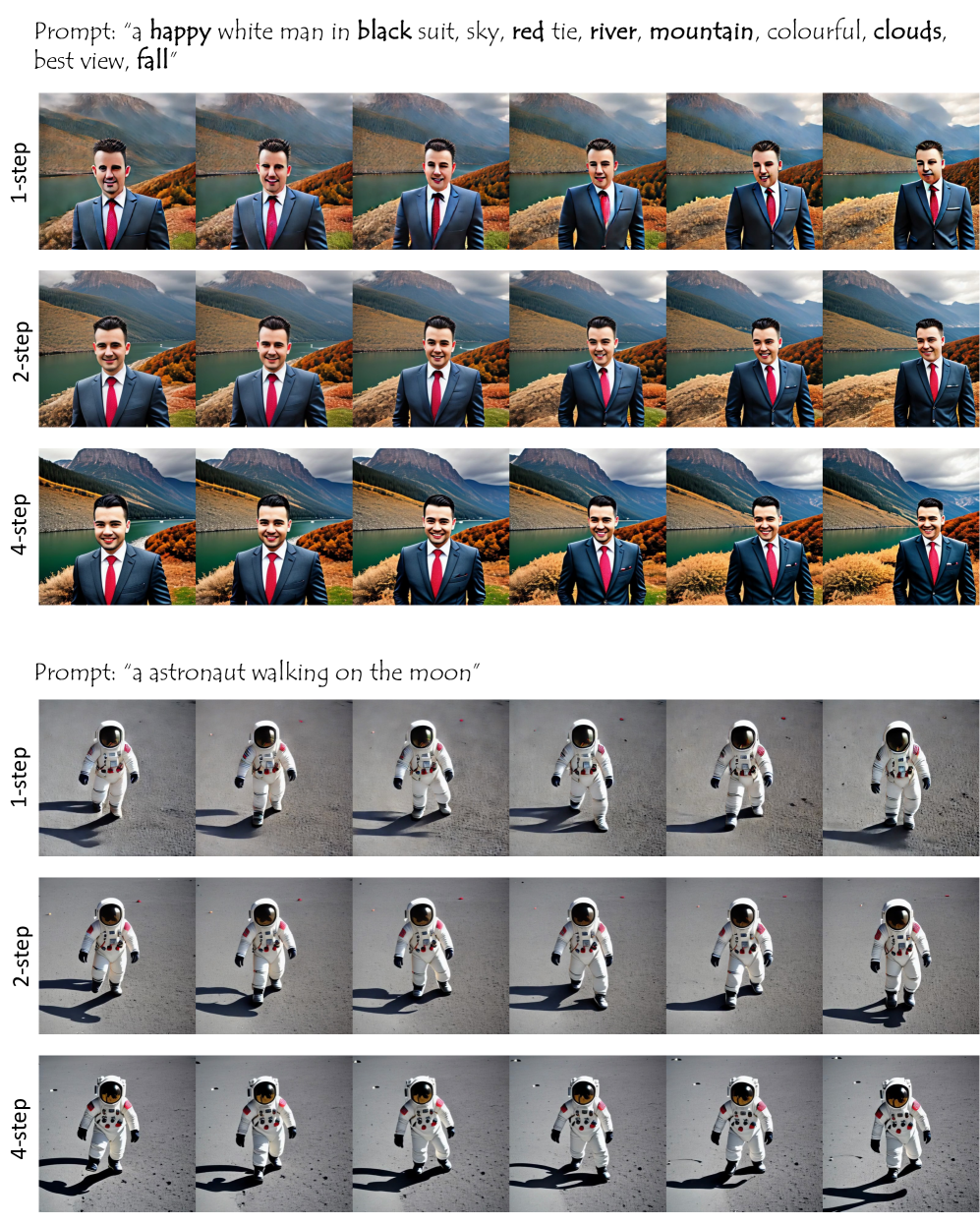
Refer to caption

Figure 10: PCM video generation results with Stable-Diffusion v1-5 under 14similar-to141\sim 4 inference steps.

Refer to caption

Figure 11: PCM video generation results with Stable-Diffusion v1-5 under 14similar-to141\sim 4 inference steps.

Refer to caption

Figure 12: PCM video generation results with Stable-Diffusion v1-5 under 14similar-to141\sim 4 inference steps.

Refer to caption

Figure 13: PCM video generation results with Stable-Diffusion v1-5 under 14similar-to141\sim 4 inference steps.

Refer to caption

Figure 14: PCM video generation results comparison with AnimateLCM under 14similar-to141\sim 4 inference steps.

Refer to caption

Figure 15: PCM video generation results comparison with AnimateLCM under 14similar-to141\sim 4 inference steps.

Refer to caption

Figure 16: PCM generation results with Stable-Diffusion v1-5 under different inference steps.

Refer to caption

Figure 17: PCM generation results with Stable-Diffusion v1-5 under different inference steps.

Refer to caption

Figure 18: PCM generation results with Stable-Diffusion XL under different inference steps.

Refer to caption

Figure 19: PCM generation results with Stable-Diffusion XL under different inference steps.

Refer to caption

Figure 20: PCM generation 1-step results with Stable-Diffusion v1-5.

Refer to caption

Figure 21: PCM generation 2-step results with Stable-Diffusion v1-5.

Refer to caption

Figure 22: PCM generation 4-step results with Stable-Diffusion v1-5.

Refer to caption

Figure 23: PCM generation 8-step results with Stable-Diffusion v1-5.

Refer to caption

Figure 24: PCM generation 16-step results with Stable-Diffusion v1-5.

Refer to caption

Figure 25: PCM generation 1-step results with Stable-Diffusion XL.

Refer to caption

Figure 26: PCM generation 2-step results with Stable-Diffusion XL.

Refer to caption

Figure 27: PCM generation 4-step results with Stable-Diffusion XL.

Refer to caption

Figure 28: PCM generation 8-step results with Stable-Diffusion XL.

Refer to caption

Figure 29: PCM generation 16-step results with Stable-Diffusion XL.

Refer to caption

Figure 30: PCM generation 16-step results with Stable-Diffusion XL.

Refer to caption

Figure 31: Visual examples of ablation study on the proposed distribution consistency loss. Left: Results generated without the distribution consistency loss. Right: Results generated with the distribution consistency loss.

[Uncaptioned image]

Refer to caption

Figure 32: Visual examples of ablation study on the proposed way for stochastic sampling. Pure deterministic sampling algorithms sometimes bring artifacts in the generated results. Adding stochasticity to a certain degree can alleviate those artifacts.

Refer to caption

Figure 33: Visual examples of ablation study on the proposed strategy for promoting diversity. Upper: Batch samples generated with prompt "a car" with normal CFG=1.0 value in 4-step. Lower: Batch sample generated with prompt "a car" with our proposed strategy with CFG=0.6.

Refer to caption

Figure 34: Visual examples of ablation study on the proposed strategy for promoting diversity. Upper: Batch samples generated with prompt "a car" with normal CFG=1.0 value in 4-step. Lower: Batch sample generated with prompt "a car" with our proposed strategy with CFG=0.6.