Scaling Laws and Compute-Optimal Training
Beyond Fixed Training Durations

Abstract

Scale has become a main ingredient in obtaining strong machine learning models. As a result, understanding a model’s scaling properties is key to effectively designing both the right training setup as well as future generations of architectures. In this work, we argue that scale and training research has been needlessly complex due to reliance on the cosine schedule, which prevents training across different lengths for the same model size. We investigate the training behavior of a direct alternative — constant learning rate and cooldowns — and find that it scales predictably and reliably similar to cosine. Additionally, we show that stochastic weight averaging yields improved performance along the training trajectory, without additional training costs, across different scales. Importantly, with these findings we demonstrate that scaling experiments can be performed with significantly reduced compute and GPU hours by utilizing fewer but reusable training runs. Our code is available at https://github.com/epfml/schedules-and-scaling/.

1 Introduction

Training large language models is expensive — in time, energy, and compute. Moreover, it requires a complex algorithmic recipe of model architecture and training data to obtain high-quality models. Therefore, the workflow of training large models consists of iterating over small experiments to verify success before extrapolating to larger scales. This is then either done by computing specialized scaling laws (OpenAI, 2023; Bi et al., 2024; Hu et al., 2024; Team et al., 2023), relying on established laws (Hoffmann et al., 2022; Anil et al., 2023) or training past compute-optimality to save cost at inference (Touvron et al., 2023a, b).

Despite large advances across data and training recipes, one aspect of large language model (LLM) pretraining has remained surprisingly prevalent: the cosine learning rate schedule (Loshchilov & Hutter, 2016; Radford et al., 2018; Rae et al., 2021). Importantly, the Chinchilla project (Hoffmann et al., 2022) showed that the cosine schedule achieves optimal loss only when the cycle length matches the training duration, but underestimates the model performance during training. This means that when performing experiments — e.g., for architectural changes or data mixtures — one must train multiple models for different lengths, from scratch, to have reliable estimates of the quality of training and the scaling behavior. This is much more expensive than training a suite of models just once. Even more, it is restrictive for the final model for which the training length must be decided in advance.

In this work, our goal is to revisit and question the necessity of the cosine learning rate schedule for large model training. Through a multitude of training runs, we demonstrate how a simple alternative of performing a cooldown after a constant learning rate — which was already suggested in the literature (Zhai et al., 2022) and recently used by released models (Hu et al., 2024; Shen et al., 2024) — matches the performance of cosine. We expand on this and provide and analyze different recipes for the decay form and length, which scale as reliable as cosine, outperforming it for sufficiently long cooldowns. Going beyond, we investigate stochastic weight averaging (Izmailov et al., 2018) and a schedule-free optimizer (Defazio et al., 2024), which give strong (but not optimal) performance at any point during training and can act as a replacement for the learning rate decay, if the performance gap is acceptable and avoiding separate cooldowns is preferred.

These findings suggest that research on training recipes and scaling laws has been needlessly complex due to the need to retrain models from scratch. We demonstrate this empirically by performing a small-scale experiment of scaling laws which only uses a fraction of the compute and GPU hours that were previously needed. Following, we discuss that this makes scaling research more accessible and enables more frequent computation of laws for data mixtures (Bi et al., 2024; Goyal et al., 2024; Aghajanyan et al., 2023) or novel architectures (Gu & Dao, 2023; De et al., 2024).

2 Background: Cosine Learning Rate Schedule for LLMs

Figure 1: Revisiting cosine optimality for language models. We revisit the observation from Chinchilla (Hoffmann et al., 2022) that in order to achieve the best model after a certain training length (tokens), the cosine schedule must match the total duration of training. This comes at the cost of neither being able to stop before or going beyond the cycle — an issue we show how to alleviate in Section 3.

Revisiting the optimality of the cosine schedule. We start our argument by revisiting the use of the cosine schedule in large language model (LLM) training. For any machine learning model, the learning rate value (LR) and schedule both are crucial choices for training. From optimization theory, our understanding is that a slow annealing of the learning rate is essential to find good minima in the loss landscape particularly for deep networks, whereas higher values help exploration (Smith et al., 2017; Loshchilov & Hutter, 2016).

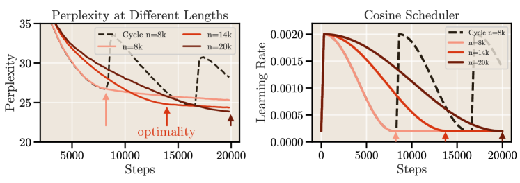
In the context of LLMs, the most commonly used cosine strategy presents a particular trade-off by which the LR reaches its maximum early after the warm-up stage and then gradually decreases, typically to 10% of the maximum LR (see Figure 1, right). Since the seminal works of GPT (Radford et al., 2018, 2019; Brown et al., 2020) and large models like Gopher (Rae et al., 2021), PaLM2 (Anil et al., 2023) or LLaMA (Touvron et al., 2023a, b), cosine has stayed the de-facto standard schedule.

Experimental visualization. Our first goal is to understand the importance of the length of the schedule for performance of the model. To this end, we implement the common decoder-only transformer (Vaswani et al., 2017) identical to the LLaMa (Touvron et al., 2023a, b) or Noam architecture (Ormazabal et al., 2024). Throughout this paper, we use the AdamW optimizer with weight decay (Kingma & Ba, 2014; Loshchilov & Hutter, 2017) with common LLM training parameters. We train on a subset of SlimPajama (Soboleva et al., 2023) with 6B tokens, a cleaned and deduplicated corpus for LLM pretraining, which we split into train and validation sequences and report validation loss (perplexity). We provide all details in Appendix A.1.

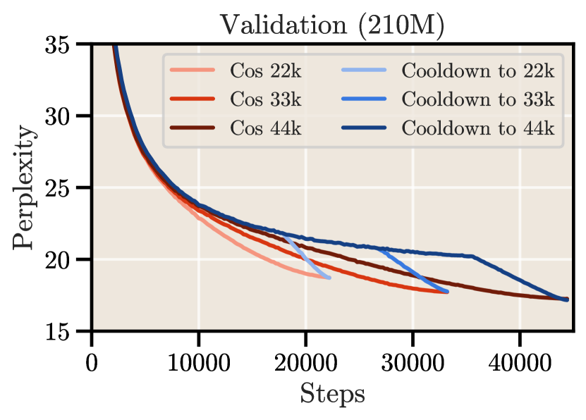
The pitfalls of cosine. In the results of Figure 1, we see that the key parameter for the cosine schedule is the length of training: At specific step counts, the best perplexity is always achieved by the cosine schedule that matches the length. This is the main observation of Hoffmann et al. (2022) — in order to achieve the best model for a specific token count, the training duration must be known in advance and match the cosine length. However, this brings particular issues. First, cosine is suboptimal during training and underestimates the model’s performance for the same token count. At the same time, cosine strongly complicates continuation of training. For example, one could easily be mistaken to extrapolate a loss curve of a cosine schedule beyond the end of the cycle. The improvement in loss precisely happens because of the LR decay; afterwards, the final learning rate will generally be too low to continue making large progress. In contrast, rewarming leads to spikes of which the training only slowly recovers, similarly reported in the continual learning literature (Ibrahim et al., 2024).

3 A Different Route: Constant Learning Rate with Cooldown

Figure 2: Illustration of schedules. Cosine (red) follows a slow decrease in learning rate, typically to 10% of the maximum for LLMs. The alternative (blue) is characterized by an aggressive decrease in learning rate via e.g. a linear cooldown.

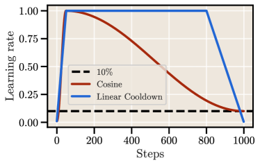
Why does the cosine schedule with a single cycle work well for LLM training? Arguably, it provides a good trade-off between a high learning rate and cooling down the model sufficiently, which is expanded proportionally to the training steps.

The alternative — constant + cooldown. The tradeoff of cosine can also be achieved by a different schedule. Here, the learning rate is kept constant for the majority of the training and only decreases in a short final phase, known as the cooldown (or decay/annealing phase). This schedule has previously been referred to as a trapezoidal (Zhai et al., 2022), and later as the warmup-stable-decay schedule (WSD) (Hu et al., 2024). To avoid overloading of terms (e.g., weight decay), we refer to this approach as constant LR + cooldown.

The cooldown phase typically has the LR go to zero linearly, mirroring the warmup phase, which gives rise to an overall trapezoidal shape (see Figure 2). Formally, we can define it as:

$$\eta(n)=\begin{cases}\frac{n}{N_{\text{warmup}}}\cdot\eta_{\text{max}}&\text{if }n<{N}_{\text{warmup}}\\ \eta_{\text{max}}&\text{if }N_{\text{warmup}}<n\leq N-N_{\text{decay}}\\ f(n,N,N_{\text{decay}})\cdot\eta_{\text{max}}&\text{if }n>N-N_{\text{decay}}\end{cases}$$ (1)

with the peak learning rate $\eta_{\text{max}}$, the total steps $N$ with warmup and cooldown steps $N_{\text{warmup}}$ and $N_{\text{decay}}$, and a monotonically decreasing function $f(n,N,N_{\text{decay}})$ that handles the cooldown.

Conceptual advantages. The main advantage of this schedule is that specifying the number of training steps in advance is not required. This is particularly convenient for large runs, as the cooldown can be initiated at any time to observe model behavior and decide whether to stop. It also allows for continual learning by default, for which training can be resumed from a checkpoint prior cooldown. Moreover, the data mixture can be changed during the cooldown phase (Hu et al., 2024) as a form of finetuning; while we focus on the same mixture, understanding the curriculum aspect of the separate phases is an important direction for future research.

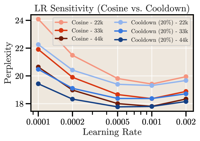
Experimental comparison. We follow our experimental setup and train a 210M parameter model on SlimPajama with constant LR and the cooldown schedule defined in (1). That is, we compare the same length of warmup and training, but replace the cosine decay after warmup with a constant LR and a cooldown for 20% of steps linearly going to zero. We additionally sweep the learning rate for both approaches. In the results shown in Figure 3, perhaps suprisingly, we observe an almost perfect match between the performance of the best cosine and cooldown schedule even for different training durations, all while exhibiting slightly less sensitivity to variations in the LR.

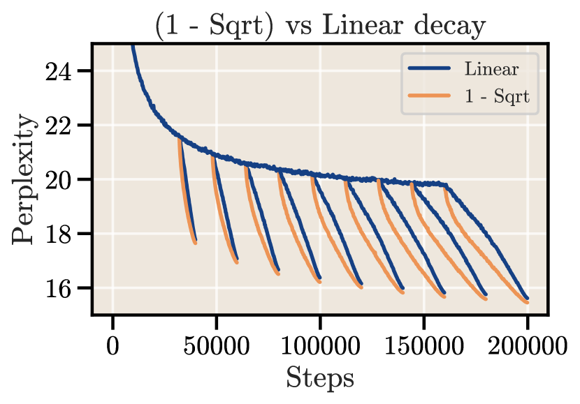
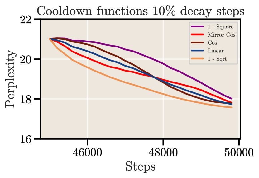
Different cooldown schedules. We investigate various functions describing the cooldown shape, including cosine, square and square root shapes in Appendix B.1. We identify a new function (1-sqrt) that outperforms the linear cooldown. This improvement is maintained in a smaller number of decay steps, different learning rates, and various timestamps (see Appendix B.1). In Figure 4, we train a model for 200K steps (approximately 20B tokens), applying cooldown every 20K steps for 20%. The results indicate that the longer the training duration, the more the linear cooldown is outperformed by the (1-sqrt) cooldown, which we define as:

$$f(n,N,N_{\text{decay}})=\textstyle\left(1-\sqrt{\frac{n-(N-N_{\text{decay}})}{N_{\text{decay}}}}\,\right)$$ (1-sqrt)

Figure 3: The difference in loss curves of cosine vs. constant learning rate with cooldown. The cooldown phase initiates a sharp decrease in loss (left) to match cosine; the training perplexity follows the same behavior (Fig. 13). We find the LR sensitivity (right) to be similar for both schedules, albeit less for cooldown, where the optimum lies slightly below at half of the optimal cosine maximum LR.

Takeaway 1: The constant LR + cooldown schedule offers significant convenience by not requiring the number of training steps to be specified in advance, and provides similar or better performance compared to the optimally tuned cosine schedule.

Takeaway 2: We introduce a cooldown form (1-sqrt) that consistently outperforms the linear decay.

Figure 4: A different cooldown schedule can improve performance. Perhaps surprisingly, we find that a different decay phase in the functional form of (1-sqrt) can consistently outperforms the standard linear decay, where both are better than a well-tuned cosine for long lengths.

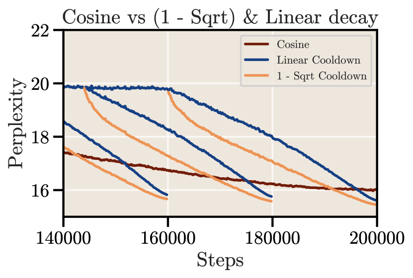
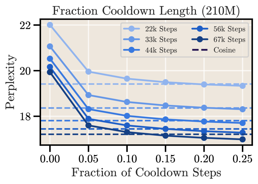
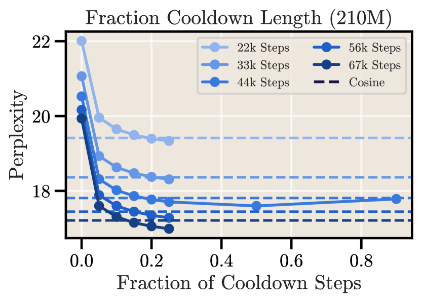
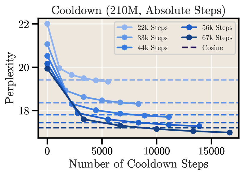
How long do you need to cooldown? To effectively utilize the schedule, it is essential to determine the optimal number of decay steps. Our study on the relative number of cooldown steps, as shown in Fig. 5, reveals that the benefits of extended cooldown periods plateau at around 20%. We select this percentage for our experiments as the model size and the number of tokens are relatively small. Additionally, in Fig. 6 we demonstrate that using only 5% decay with the (1-sqrt) cooldown can nearly match the performance of the cosine schedule on a 20B token run (much beyond Chinchilla optimal).

Figure 5: Longer cooldown helps to achieve lower loss. We investigate the effect of the cooldown length as a fraction of the total steps for both the 210M model (left) and 60M (right). For a well-tuned learning rate of cosine, we find that the cooldown surpasses cosine between 10-20% of steps (left), but stops improving when done over a majority of training. This also holds when sweeping the learning rate (right). Additional ablations are provided in Appendix B.1.

Figure 6: A long training run suggests that a small number of cooldown steps can match cosine for long training. From Fig. 5 and Fig. 17, we find that the required duration of cooldown to match the cosine loss decreases with longer training; we validate with a long training run (200k steps), and find that just 10k cooldown steps almost perfectly match cosine in performance.

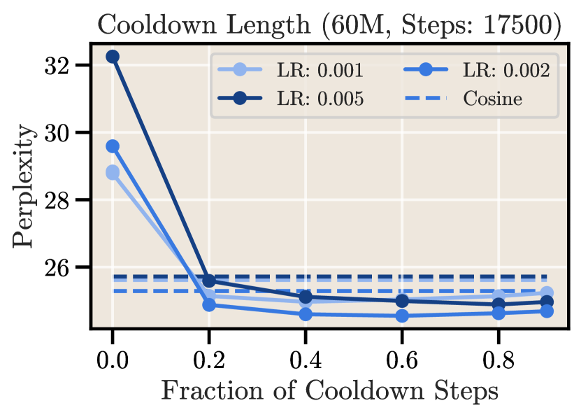
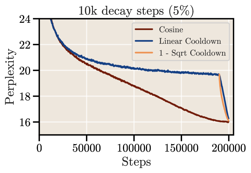
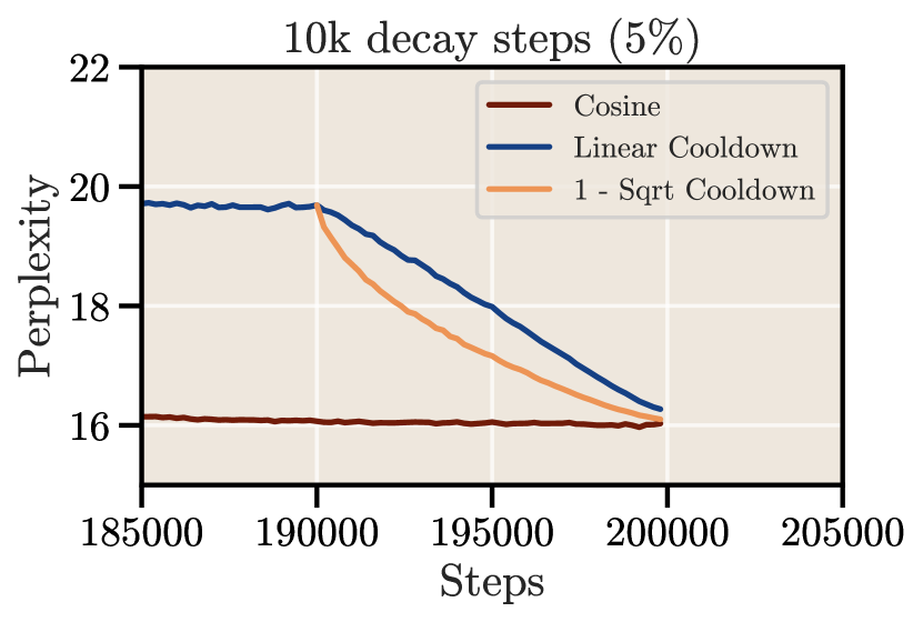
Takeaway 3: The constant learning rate with a short cooldown (< 20% of total training steps) achieves the same final loss as a well-tuned cosine schedule, and only outperforms for a longer fraction of cooldown steps. For long training runs, our results suggest that the cooldown length can be less than 20% to match cosine if enough in absolute steps — see Figure 6.

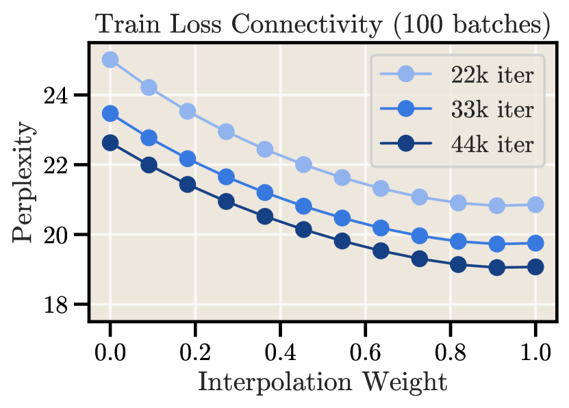
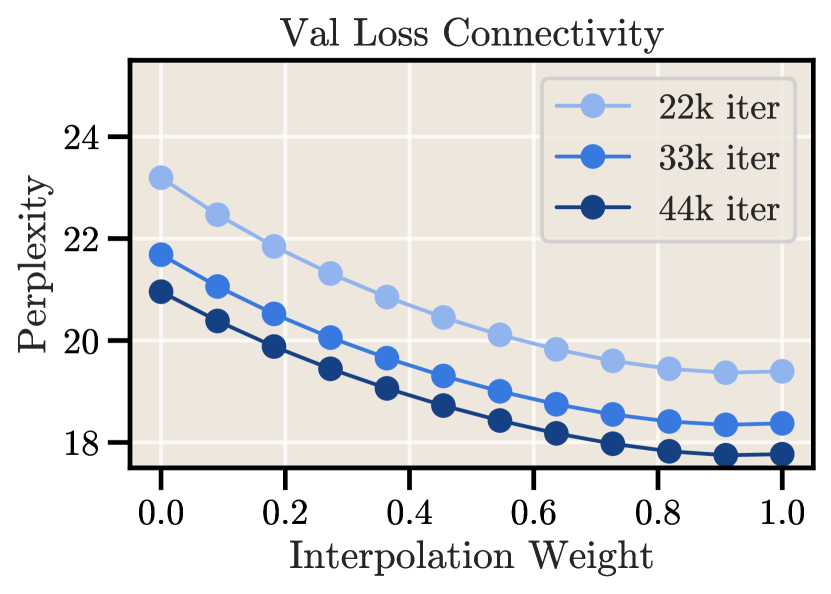
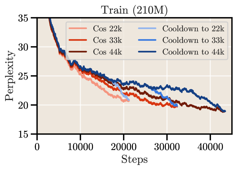
What happens during the cooldown? It is remarkable how the sudden drop in loss is consistent for both train and validation loss and aligns closely with the decay in learning rate (Figure 13). Hu et al. (2024) investigate the cooldown phase and find that the first-order directional derivative diminishes with each step, whereas the curvature of the loss function increases; they attribute this to proximity to a local optimum.

We expand upon these results and aim to understand the optimization landscape around the trajectory of the cooldown. For that, we evaluate the loss along the straight line trajectory when moving between a checkpoint before and after cooldown, i.e., a linear interpolation of the two models’ weights. Perhaps surprisingly, we find that the smooth drop in loss also occurs for this interpolation, as visualized in Figure 7. This aligns with the findings of Hu et al. (2024). These results suggest that upon decaying the learning rate, the model immediately descends into a connected minimum of the loss.

Takeaway 4: The cooldown phase is a smooth transition to a basin in the loss landscape.

Figure 7: The smooth drop in loss also occurs when moving linearly in weight space between checkpoints before and after the cooldown. This suggests that in the cooldown phase, the model directly moves within a connected basin in the loss landscape.

4 Do We Even Need to Cooldown?

In Section 3, we showed that a constant LR with a short cooldown phase can replace the cosine decay. Ideally, however, we would not need a decay at all, but aim to obtain an optimal model at any point in training even when prolonged. This would save even more computational resources and time. In this section, we investigate two potential approaches: weight averaging and a schedule-free optimizer.

4.1 Stochastic Weight Averaging (SWA)

Motivation. While slow annealing of the learning rate can be essential to find good minima (Smith et al., 2017; Loshchilov & Hutter, 2016), Sandler et al. (2023) show theoretical and empirical equivalence between stochastic weight averaging (SWA) and cooldown schedules in training vision models. There, averaging intuivitely and naturally reduces noise and thereby improves generalization. Motivated by these results, we aim to answer the same question in LLM training: Can weight averaging replace the cooldown phase?

Method. We opt for a form of SWA (Izmailov et al., 2018) that splits the training in fixed windows and averages within a window, which allows to keep the average as a single additional copy of the model parameters. In our experiments, we set the window to $h=500$ steps and save checkpoints every $h$ steps, which allows evaluating longer windows ad-hoc to see potential improvements akin to latest weight averaging (LAWA, Kaddour, 2022; Sanyal et al., 2023). For all our experiments, we find that windows below or at 2500 steps (256M tokens) are optimal. We also experimented with an exponential moving average (EMA), which performed worse than SWA, and therefore do not report EMA.

Experimental results. We evaluate SWA in the same setup of the 210M model and show the results in Fig. 8 for both a constant LR (left) and cosine (right). Notably, we find a significant performance boost for SWA on top of a constant LR. Yet, it does not reach the loss values of cooldowns at intermediate steps. On the other hand, in line with previous work (Kaddour, 2022; Sanyal et al., 2023), we see a similar boost for SWA on top of a cosine schedule. This suggests that SWA, regardless of schedule, provides a compelling approach to achieving strong models along the data-scale axis that can serve as a replacement for models trained with less steps, if the performance gap is acceptable and one wishes to avoid cooldowns. This is particularly advantageous as it can arguably be done for free on top of existing and well-tuned optimizers.

Figure 8: SWA improves generalization and simulates decayed learning rates. Using SWA for the constant LR phase (left) strongly boosts the loss, but a gap to the cooldown remains. SWA also improves the generalization of a cosine schedule (right), where the intermediate checkpoints of SWA largely overlap with optimal loss trajectory of shorter cosine runs.

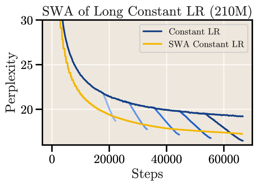
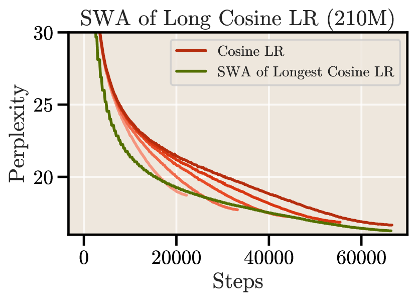
Takeaway 5: Irrespective of the schedule and without additional overhead, SWA improves performance along the training trajectory and provides better models during training. While it does not match the cooldown, it reduces the gap without the need for a separate decay phase.

Figure 9: The cooldown schedule outperforms SFO even when tuning momentum parameters. We find that SFO is sensitive to the choice of $(\beta_{1},\beta_{2})$ momentum parameters. It gives strong performance for well-tuned momentum, but falls short of cooldown.

4.2 Schedule-Free Optimizer (SFO)

Very recently, Defazio et al. (2024) introduced a schedule-free optimizer (SFO) which uses an interpolation between standard averaging and Polyak-Ruppert averaging, inspired by Nesterov’s accelerated method (Nesterov, 1983). As such, the optimizer does not require a decreasing learning rate schedule, making it relevant for continual training. We seek to investigate if it can outperform the presented cooldown schedule and provide a comparison in the same LLM setting.

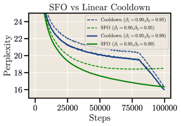
Results. We compare the results of a long 210M model run with cooldown vs. SFO with AdamW in Figure 9. While the optimizer does not require a learning rate schedule, the authors point out that training is more sensitive to the choice of the $(\beta_{1},\beta_{2})$ momentum parameters (which are not identical to the momentum in Adam). They note that the optimal parameters may depend on the length of training, making it not fully schedule free. We observe this sensitivity in our experiments, where the choice of $(0.9,0.95)$ performs notably worse and even increases loss towards the end of training. For $(\beta_{1}=0.95,\beta_{2}=0.99)$, SFO performs remarkably well. Nonetheless, both settings are matched or outperformed by the cooldown schedule, in particular when comparing the same configuration of momentum. We did not perform further hyperparameter tuning for either method.

5 The Implications for Scaling Law Research

Our investigation shows the efficacy of a constant LR for flexible training of LLMs by introducing a short cooldown phase at any point during training. In this section, we go beyond a single model, and focus on the reliability of the alternative LR schedule compared to cosine across model sizes and scales. Ultimately, we discuss the importance for the future of scaling law experiments.

Importance of scaling laws. At their core, scaling laws aim to establish a functional form of a model’s performance, commonly modelled as the loss $L$, as a function of the parameters $N$ or training tokens $D$; for LLMs, this is usually expressed as the power law

$$L(N,D)=\frac{A}{N^{\alpha}}+\frac{B}{D^{\beta}}+E\;,$$

where $\{A,\alpha,B,\beta,E\}$ are variables to be estimated (Kaplan et al., 2020; Hoffmann et al., 2022). Such scaling laws serve a multitude of critical purposes — from optimally spending a fixed amount of compute (FLOPs) for achieving the lowest loss, to trading off data-sources of different quality (Bi et al., 2024; Goyal et al., 2024) or modalities (Aghajanyan et al., 2023), to comparing the efficiency of different architectures (Gu & Dao, 2023; De et al., 2024).

Crucially, Hoffmann et al. (2022) demonstrated that is necessary to vary the number of training steps (tokens) for a fixed family of models. At the time, their results suggested that LLMs were over-sized, leading to a substantial increase in data collection and training for much longer, beyond the Chinchilla optimal point $(N,D)$ (Touvron et al., 2023a, b).

Why do the presented results matter for scaling? Following the results of Chinchilla, scaling laws require a family of models each trained from scratch with a cosine schedule that is fit to different training lengths (cf. Section 2). In contrast, the cooldown schedule as well as weight averaging allow a much cheaper alternative in two phases: first, a model sweep with a single sufficiently long training run for each model size in the family; then, using the model checkpoints to perform a cooldown or averaging. This reduces scaling law experiments to only the model scaling axis, effectively dividing the number of necessary training runs by one order of magnitude. At the same time, it allows for flexible continual training beyond any predetermined number of steps.

Experimental setup. We mimic a small-scale experimental setup for scaling laws: We train a range of model sizes (33M-360M) across different token scales (0.3B-10B) on the same SlimPajama 6B dataset. For each model, we choose exactly three token counts (around the Chinchilla optimal ratio of D/N=20) in increments of 10, 20 and 30 tokens per parameter. With the cosine schedule, each model is trained from scratch three times. In contrast, for averaging, we train each model just once for the longest cycle, then use the averages at the same token count as cosine; for cooldown, we similarly take checkpoints along the constant LR trajectory and perform three annealing periods to match the token counts. We adjust the LR to be higher for smaller models. In line with the findings of Sect. 3 and for a fair comparison, we set the constant LR to be half of the maximum LR for cosine and perform 20% (linear) cooldown steps as the longest runs are below 70k steps. More details are given in Appendix A.1.

Results. We show the validation loss envelopes as a function of the training FLOPS in Fig. 10 (left) and compare each obtained model (i.e., same parameter & tokens) with cosine and its alternatives (right). We find that the cooldown learning rate schedule scales reliably, much like cosine and SWA, to achieve optimal losses with the recipe we establish in previous sections. This is particularly visible in Fig. 10 (right), where each model’s performance lies almost perfectly on the diagonal, which signals that cosine (y-axis) and cooldown (x-axis) reach the same loss after the same amount of tokens. A similar result is visible for SWA, though the reciprocal (y-offset) is negative, which agrees with our findings from Sect. 4.1 that the averaging does not fully close the gap to a LR cooldown.

Compute savings. Crucially, the alternatives enable scaling laws for just a fraction of the cost. In Fig. 11(a), we report FLOPS and GPU hours (real wall-clock time) for all model runs for both methods. They substantially reduce both compute and GPU hours. In our experiments, where we space the runs to use token ratios of $10,20$ and $30$, it saves half the time and FLOPS, enabling scaling laws for only a fraction of the previous cost. We report the detailed savings for all models in Appendix B.3.

Figure 10: Cooldown LR schedule + SWA scale reliably. To validate our findings, we launch a range of model sizes (33M-360M), each for three different cosine cycle lengths. For the other methods, we train each model just once for the longest cycle and take the snapshots at the same token count as cosine (for SWA) or perform post-train cooldowns to the same length. Each final models is represented by a dot. Left: The loss curve envelopes. Right: The perplexity of cosine (y-axis) vs. cooldowns and SWA. Points on the diagonal indicate the same loss for both methods; above outperforming cosine, below fall short. We see alignment between both methods.

(a) FLOPS and GPU hours for our models.

	FLOPS
Chinchilla	$5.59\times 10^{23}$
w/ Cooldown	$2.36\times 10^{23}$

(a) Estimated FLOPS savings for Chinchilla.

Figure 11: Scaling laws for a fraction of the cost. The reliable behavior of both the cooldown schedule and SWA allows scaling experiments with a drastic reduce in both compute and GPU hours; in both our experiments (left) and the original Chinchilla (right) a factor of $\frac{1}{2}$ or less. The more training runs are performed per model size (e.g. 4 for Chinchilla), the larger the difference becomes.

Estimating savings for Chinchilla. We take our analysis further and estimate how much cheaper the Chinchilla model suite would have been if performed with 10% cooldowns after a single run for each model size using the model configurations as reported in Table A9 (Hoffmann et al., 2022). Since the authors do not report exact training configurations, we consider a sequence length of 1024, a batch size of 0.5M tokens and token ratios $M=D/N\in\{10,15,20,25\}$ for each model. With this, we arrive at roughly $5.59\times 10^{23}$ total FLOPS originally vs. $2.36\times 10^{23}$ (Figure 1(a)). This means that less than half the compute could have been used.

Takeaway 6: Scaling experiments can be done with significantly reduced compute and GPU hours by utilizing fewer but reusable training runs with a constant learning rate and ad-hoc cooldowns.

Additional results. We plot the training curves of all models in Appx. B.2. In addition, we show that our findings transfer to different datasets with experiments on OpenWebText2 in Appx. B.4.

6 Limitations

We conduct our experiments on models of up to 360M, training on up to 10B tokens. The trends we find are consistent across all scales, but the behavior may change at modern scales (Wei et al., 2022; Tay et al., 2021). Nonetheless, the approach of a constant learning rate followed by a cooldown has already proven successful at larger scales for released models (Hu et al., 2024; Shen et al., 2024; Zhai et al., 2022). Similarly, instabilities arising from a high learning rate for a long part of training can be alleviated (Wortsman et al., 2023). We therefore do not see any intrinsic barriers to the method at scale.

Secondly, we exclusively focus on the training or validation loss, though downstream tasks are ultimately the main metric of interest. While they often scale reliably with the loss (Du et al., 2024; Gadre et al., 2024), this remains an important question for further research; in particular, when coupled with different data-mixtures during the cooldown phase, as is the focus of (Hu et al., 2024; Shen et al., 2024) and out of the scope of our work.

7 Related work

Cosine Schedules and Alternatives for Transformers. The cosine decay was originally introduced by Loshchilov & Hutter (2016) for cyclic schedules in vision tasks, where it is common practice to have stepwise or cyclic LRs to escape bad minima when training multiple epochs (Smith et al., 2017). For language models where data is more vast, the cosine schedule with a single cycle is currently the de-facto standard for training, with few exceptions of T5 (Raffel et al., 2020) and PaLM1 (Chowdhery et al., 2023) that used a form of inverse square root. In line with our work, recently released models opt for alternatives such as stepwise schedules (Bi et al., 2024) or the presented constant + cooldown (Shen et al., 2024; Hu et al., 2024). These alternatives were previously also explored for vision transformers by Zhai et al. (2022), who find reciprocal square-root with cooldown to perform best, and in the context of continual learning (Ibrahim et al., 2024; Gupta et al., 2023). Defazio et al. (2023) investigate the gap between theory and practice of learning rate schedules and suggest that a linear decay is optimal, also for LLM training. We similarly find that a long linear decay can slightly outperform cosine.

Weight Averaging. Weight averaging over past iterates (Polyak & Juditsky, 1992) has long been known to be beneficial for convergence. Izmailov et al. (2018) introduce stochastic weight averaging for better generalization in deep learning models. Similarly, exponential moving average is commonly used in vision (Morales-Brotons et al., 2024). Importantly, Sandler et al. (2023) show equivalency of WA to decaying learning rate schedules. In the context of LLM training, close to our work is Sanyal et al. (2023) which showed that a form of latest averaging (Kaddour, 2022) can be used to improve the performance of models early in training. However, they did not investigate the relation of weight averaging to compute optimality and its implications for scaling experiments.

Scaling Law Experiments for Neural Language Models. Kaplan et al. (2020) were the first to establish scaling laws for language models by training a suite of models for a fixed token count. Important to our work, Hoffmann et al. (2022) revise these findings and demonstrate specific methods to establish scaling laws, notably training a family of models for different cosine lengths. The subsequent models like LLama and LLama2 (Touvron et al., 2023a, b) further improve performance of smaller models by training beyond the Chinchilla optimal point, motivated by lower inference costs (Gadre et al., 2024; De Vries, 2023; Sardana & Frankle, 2023). Recent works (Muennighoff et al., 2023; Bi et al., 2024; Goyal et al., 2024) highlight how data repetition and quality affect the scaling behavior, which suggests that scaling laws should be updated more frequently. However, these works do not consider efficient experiments for scaling laws, which is the focus of our work.

8 Conclusion

We have demonstrated the reliability of an alternative learning rate schedule to replace cosine for LLM training, which uses a constant rate with a cooldown phase. Across a multitude of experiments, we analyze different recipes for the decay form and length. Importantly, we do not claim to have established the best learning rate schedule — instead, we investigate and demonstrate how an arguably simple recipe can match the performance of the current best practice of cosine, and discuss how it provides compelling advantages such as continual training and a strong reduction in costs for scaling law research. In addition, we find that SWA can give reliable (strong, but not optimal) estimates of models during runs, without additional overhead or training.

We believe the results are of great importance to the present and future of LLM training: the presented methods facilitate research for the current post-Chinchilla era, where models are trained much beyond compute-optimal, by allowing more flexibility to continue training whenever needed. At the same time, recent results that suggest data-dependency in scaling (Bi et al., 2024; Goyal et al., 2024; Aghajanyan et al., 2023; Pandey, 2024) imply the need to frequently update scaling laws, which is economically more feasible with reduced costs. We therefore hope that our work will make scaling research more accessible to researchers and practitioners alike.

Appendix A Experimental Details

A.1 Overview

Architecture and Training Parameters. We implement the most commonly used decoder-only architecture with SwiGLU activations (Shazeer, 2020), RoPE embeddings (Su et al., 2024), RMSNorm (Zhang & Sennrich, 2019) and alternating attention and MLP blocks. Unless otherwise noted, we follow standard practices in LLM training and use the AdamW optimizer with beta parameters $(\beta_{1},\beta_{2})=(0.9,0.95)$, decoupled weight decay of $0.1$ (Kingma & Ba, 2014; Loshchilov & Hutter, 2017) and gradient clipping with $1.0$. For warmup steps, we use a short warmup of $300$ steps for the majority of runs and $1000-3000$ for longer runs (above 100k total steps). The cosine schedule decays the learning rate to 10% of the maximum learning rate. For most of our experiments, we use a batch size of 200, i.e., roughly 0.1M tokens for a sequence length of 512. The vocabulary is based on the GPT-2 tokenizer (Radford et al., 2019) and contains 50304 tokens.

Dataset and Evaluation. Our main body focuses on results using SlimPajama (Soboleva et al., 2023), a cleaned and deduplicated corpus that includes webcrawl, code, papers and other sources, which is commonly used for pretraining LLMs. We use a subset of the full corpus that comprises roughly 6B tokens and randomly sample a validation set of roughly 3M tokens. During training, we evaluate the models with a fixed set of 32 batches of sequence length 512 (the same context length as training) to establish validation loss curves. At the end of training, we compute the full validation set perplexity. We perform further experiments that verify our main findings with OpenWebText2 (Gao et al., 2020) in Appx. B.4.

Implementation and Infrastructure. Our code is based on an extension of NanoGPT and uses PyTorch (Paszke et al., 2017) as well as FlashAttention (Dao et al., 2022). We incorporate the bfloat16 for memory and throughput, trained with mixed precision float32 parameters and bfloat16 activations (Micikevicius et al., 2017). All our experiments were performed using a cluster of A100 GPUs (both 40GB/80GB RAM) with 2 data-parallel (i.e., 2 GPUs per run). A few selected runs used a single node of 8 H100s. We estimate that the full cost of all experiments for this project (including prototyping) amounts to roughly 2500 GPU hours.

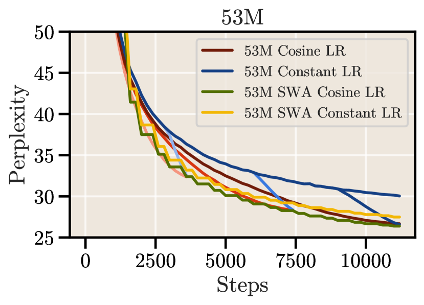
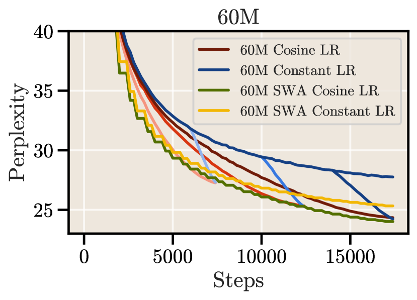
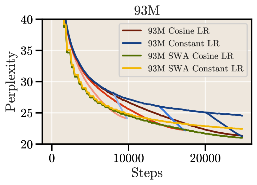
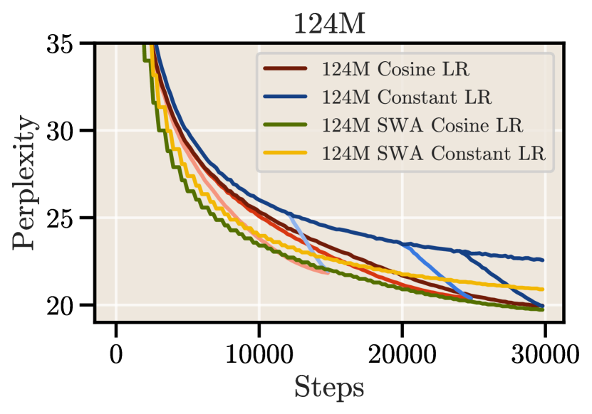
Model Configurations. We provide an overview of the model sizes and configurations in Table 1 and the parameters for training and length in Table 2. All models for the scaling law experiments are trained with 300 warmup steps and a sequence length of 512.

Model Size	d_model	n_layers	ffw_size	kv_size	n_heads
33M	384	8	1024	64	6
53M	512	8	1536	64	8
60M	512	10	1536	64	8
93M	640	12	1792	64	10
124M	768	12	2048	64	12
151M	768	16	2048	64	12
210M	768	24	2048	64	12
360M	1024	24	2816	64	16

Table 1: Model configurations. We provide an overview of the model sizes and hyperparameters for the different models in the scaling experiments.

Model	LR (Cos/Const)	Batch Size	Steps	Tokens	Token/Params Ratio
33M	(2e-3, 1e-3)	0.1M	[3k, 7k, 10k]	[0.3B, 0.7B, 1.0B]	[9.2, 21.4, 30.6]
53M	(2e-3, 1e-3)	0.1M	[3.7K, 7.5K, 11.2K]	[0.4B, 0.8B, 1.2B]	[7.2, 14.5, 21.7]
60M	(2e-3, 1e-3)	0.1M	[7.5K, 12.5K, 17.5K]	[0.8B, 1.3B, 1.8B]	[12.8, 21.4, 30.0]
93M	(2e-3, 1e-3)	0.1M	[10K, 17.5K, 25K]	[1.0B, 1.8B, 2.6B]	[11.0, 19.2, 27.5]
124M	(1e-3, 5e-4)	0.1M	[15K, 25K, 35K]	[1.5B, 2.6B, 3.6B]	[12.4, 20.7, 29.0]
151M	(1e-3, 5e-4)	0.1M	[25K, 37.5K, 50K]	[2.6B, 3.8B, 5.1B]	[16.9, 25.3, 33.7]
210M	(1e-3, 5e-4)	0.1M	[37.5K, 50K, 62.5K]	[3.8B, 5.1B, 6.4B]	[18.4, 24.6, 30.7]
360M	(1e-3, 5e-4)	0.2M	[25K, 37.5K, 50K]	[5.1B, 7.7B, 10.2B]	[14.2, 21.3, 28.5]

Table 2: Training parameters for scaling experiments. We describe the learning rates, training lengths and ratios for the different models in the scaling experiments.

A.2 FLOPS computation

We do not rely on the heuristic of 6=ND for computing the FLOPS of a Transformer model, but use a more thorough computation that involves the embeddings, attention and MLP operations directly. For reproducibility and other researchers to use, we provide our Python code in Figure 12.

⬇

1def embedding(seq_len, vocab_size, d_model):

2 return 2 * seq_len * vocab_size * d_model

3

4def attention(seq_len, d_model, key_size, num_heads):

5 projections = 2 * 3 * seq_len * d_model * (key_size * num_heads)

6 logits = 2 * seq_len * seq_len * (key_size * num_heads)

7 softmax = 3 * num_heads * seq_len * seq_len

8 softmax_query_reduction = 2 * seq_len * seq_len * (key_size * num_heads)

9 final_layer = 2 * seq_len * (key_size * num_heads) * d_model

10 return projections + logits + softmax + softmax_query_reduction + final_layer

11

12def dense(seq_len, d_model, ffw_size, swiglu=False):

13 if swiglu:

14 return 2 * seq_len * (3 * d_model * ffw_size)

15 else:

16 return 2 * seq_len * (2 * d_model * ffw_size)

17

18def final_logits(seq_len, d_model, vocab_size):

19 return 2 * seq_len * d_model * vocab_size

20

21def flops(

22 n_layers,

23 seq_len,

24 vocab_size,

25 d_model,

26 key_size,

27 num_heads,

28 ffw_size,

29 swiglu=True,

30):

31 flops_single = (

32 embedding(seq_len, vocab_size, d_model)

33 + n_layers

34 * (

35 attention(seq_len, d_model, key_size, num_heads)

36 + dense(seq_len, d_model, ffw_size, swiglu=swiglu)

37 )

38 + final_logits(seq_len, d_model, vocab_size)

39 )

40 # assume backward pass has twice the FLOPs of the forward pass

41 return 3 * flops_single

Figure 12: FLOPS computation. Instead of the common approximation of 6=ND, we use more detailed calculations for the FLOPs estimation based on the Transformer model configuration. We provide the Python code above.

Appendix B Additional Results

Figure 13: The difference in loss curves of cosine vs. constant learning rate with cooldown. The cooldown phase initiates a sharp decrease in loss for both training (left) and validation (right). The training perplexity is averaged out over a window to achieve a smoother curve. For validation, we use a fixed set of 32 validation batches to report the loss each step, which creates a smooth curve by design.

B.1 More Results on Cooldown

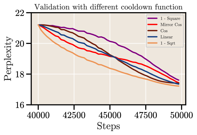
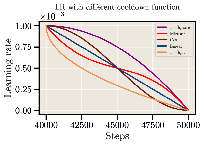
Ablation of functional form of cooldown. We provide additional experiments to show that our results are consistent and robust to different changes. For simplicity, we only cooldown to 50K steps here, but we found these results hold regardless of the step at which we decay. In Fig. 14 and Fig. 15, we test different functions for the cooldown phase:

• Linear: Classical linear decay.

• 1 - Sqrt: Defined in Eq. (1-sqrt).

• Cosine: Similar to the classical cosine decay, but applied only during the decay phase.

• Mirror Cosine: The symmetric counterpart of the cosine function with respect to the linear decay.

• 1 - Square: The square root function in Eq. (1-sqrt) is replaced by a square function.

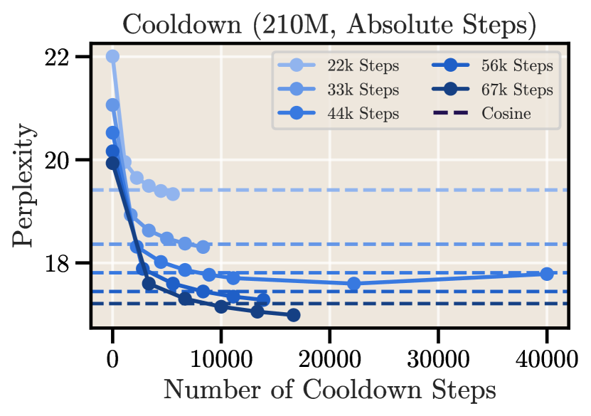
Length of cooldown. We repeat our ablation from Sect. 3 in Figure 16 with the absolute number of decay steps (not fractional) in Figure 17.

Figure 14: Different cooldown functions. We test various cooldown schedule functions and consistently observe the same order of performance (left), with (1-sqrt) being the most effective. Remarkably, the drop in loss closely follows the learning rate (right) even for different functions.

Figure 15: The order and results of different cooldowns hold across settings. Left: We change the learning rate to $5e^{-4}$ instead of $1e^{-3}$ as in previous experiments. Right: The performance for 10% cooldown steps instead of 20%.

Figure 16: Parabola shape of the relationship between cooldown length and final perplexity. We repeat the plots from Fig. 5 with a zoomed-in view on the left.

Figure 17: The effect of the cooldown length in terms of absolute steps. We repeat the plots from Fig. 5 with the absolute number of steps on the x-axis.

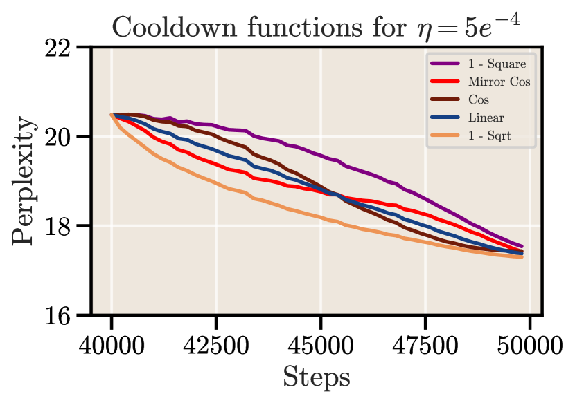
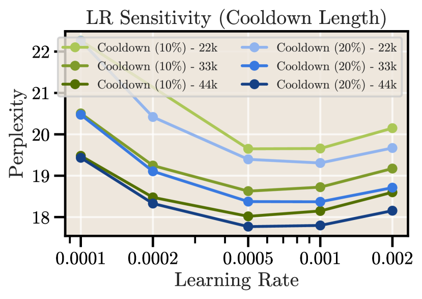
LR sensitivity. The optimal learning rate also transfers to different cooldown lengths in our experiments, see the results in Figure 18.

Figure 18: Learning rate sensitivity for cosine and cooldown with different lengths. The optimal learning rate also transfers to different cooldown lengths.

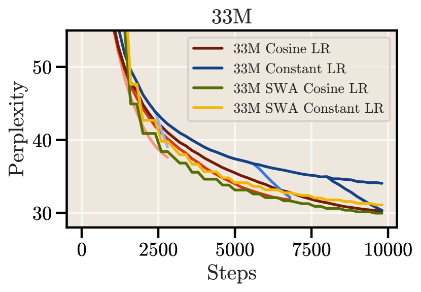
B.2 Learning Curves for All Models of Scaling Experiments

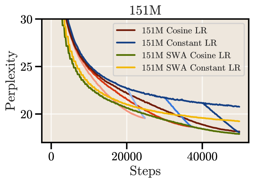
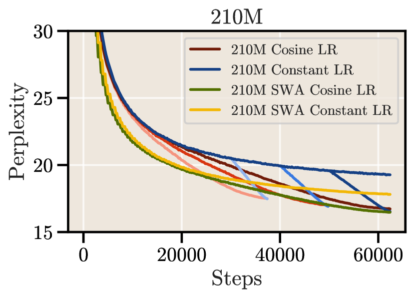
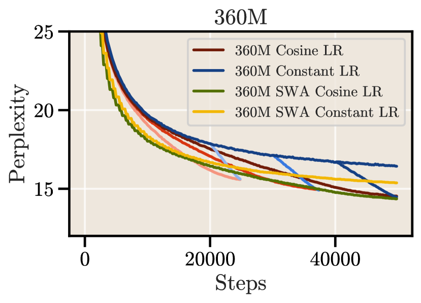
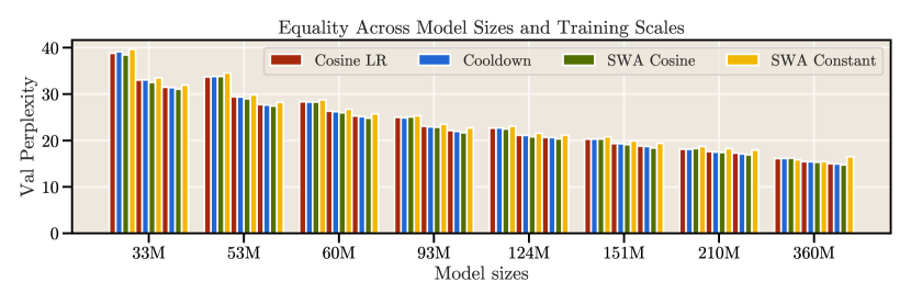
We provide the learning curves for all models in the scaling experiments in Figure 19. The final validation perplexity for all models and methods is given in Figure 20.

Figure 19: Validation Loss Curves (Perplexity) of all Models in Scaling Experiments. We visualize all training runs for the models used in the scaling experiments in Section 5.

Figure 20: Final Validation Perplexity of all Models in Scaling Experiments across different Runs.

B.3 Additional Results and Compute Savings.

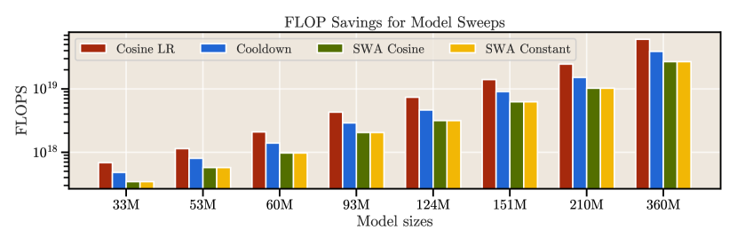
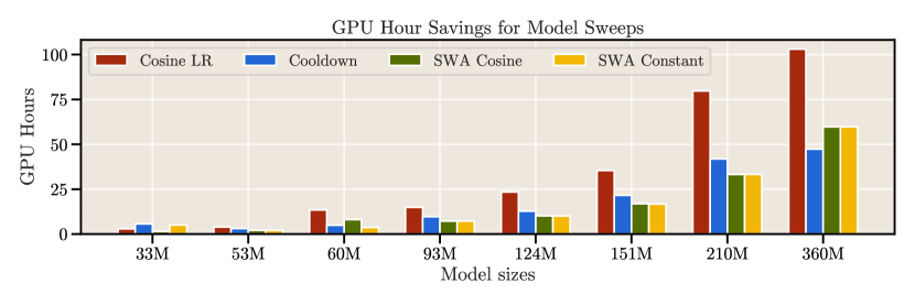
We give the savings for all models used in the scaling experiments in terms of FLOPS in Figure 21 and GPU hours in Figure 22.

Figure 21: FLOPS Savings for all Models in Scaling Experiments across different Runs (Log Scale). The FLOPS savings amount to a factor of $\frac{1}{2}$ across all models. If more runs across different lengths were to be performed (e.g., 3 per model in our experiments), the difference becomes more significant.

Figure 22: GPU Hours Savings for all Models in Scaling Experiments across different Runs. We report the actual runtimes summed up over the sweeps for all models. The savings in terms of runtime become especially more prominent for bigger models and longer training runs. Please note that the hours for SWA of the 360M model are slightly off because of congestion in our cluster during the runs.

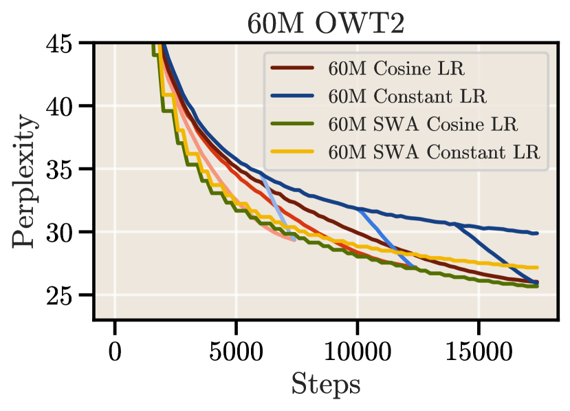
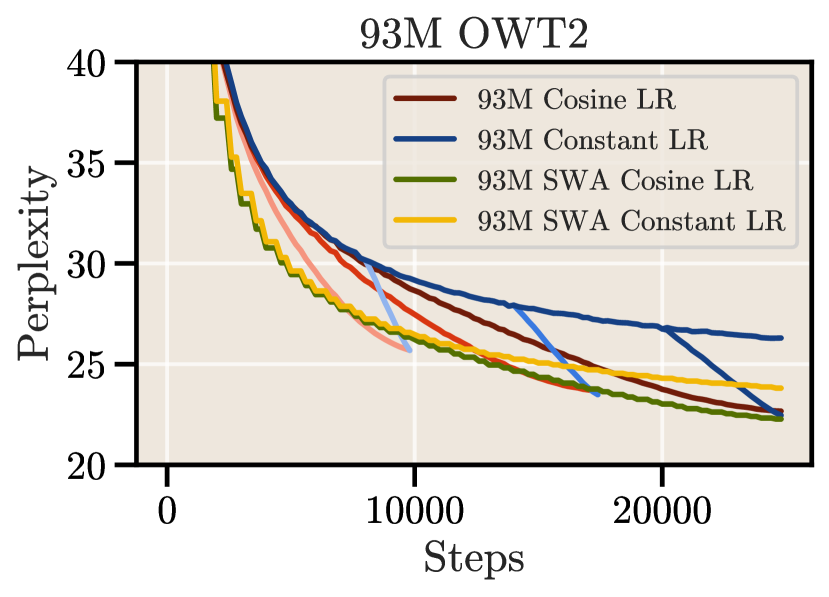
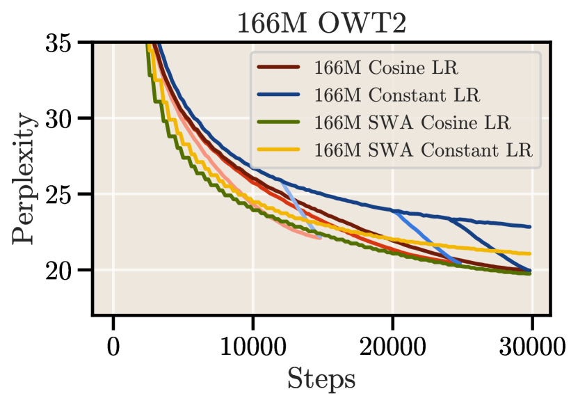
B.4 Additional Experiments on OpenWebText2

In addition to all results on SlimPajama, we perform experiments on the commonly used benchmark of OpenWebText2 (Gao et al., 2020) with models of sizes 60M, 93M and 166M. As shown in Figure 23, our findings from previous experiments succesfully transfer, where the cooldown recipe matches the performance of cosine and SWA boosts performance during training.

Figure 23: Results Transfer to OpenWebText2. We see the same behavior for cooldown schedules and SWA, verifying the reliability of the alternative training methods.

References

- Aghajanyan et al. (2023) Aghajanyan, A., Yu, L., Conneau, A., Hsu, W.-N., Hambardzumyan, K., Zhang, S., Roller, S., Goyal, N., Levy, O., and Zettlemoyer, L. Scaling laws for generative mixed-modal language models. In International Conference on Machine Learning, pp. 265–279. PMLR, 2023.
- Anil et al. (2023) Anil, R., Dai, A. M., Firat, O., Johnson, M., Lepikhin, D., Passos, A., Shakeri, S., Taropa, E., Bailey, P., Chen, Z., et al. Palm 2 technical report. arXiv preprint arXiv:2305.10403, 2023.
- Bi et al. (2024) Bi, X., Chen, D., Chen, G., Chen, S., Dai, D., Deng, C., Ding, H., Dong, K., Du, Q., Fu, Z., et al. Deepseek llm: Scaling open-source language models with longtermism. arXiv preprint arXiv:2401.02954, 2024.
- Brown et al. (2020) Brown, T., Mann, B., Ryder, N., Subbiah, M., Kaplan, J. D., Dhariwal, P., Neelakantan, A., Shyam, P., Sastry, G., Askell, A., et al. Language models are few-shot learners. Advances in neural information processing systems, 33:1877–1901, 2020.
- Chowdhery et al. (2023) Chowdhery, A., Narang, S., Devlin, J., Bosma, M., Mishra, G., Roberts, A., Barham, P., Chung, H. W., Sutton, C., Gehrmann, S., et al. Palm: Scaling language modeling with pathways. Journal of Machine Learning Research, 24(240):1–113, 2023.
- Dao et al. (2022) Dao, T., Fu, D., Ermon, S., Rudra, A., and Ré, C. Flashattention: Fast and memory-efficient exact attention with io-awareness. Advances in Neural Information Processing Systems, 35:16344–16359, 2022.
- De et al. (2024) De, S., Smith, S. L., Fernando, A., Botev, A., Cristian-Muraru, G., Gu, A., Haroun, R., Berrada, L., Chen, Y., Srinivasan, S., Desjardins, G., Doucet, A., Budden, D., Teh, Y. W., Pascanu, R., Freitas, N. D., and Gulcehre, C. Griffin: Mixing gated linear recurrences with local attention for efficient language models. Feb 2024. URL http://arxiv.org/abs/2402.19427v1.
- De Vries (2023) De Vries, H. Go smol or go home, 2023. URL https://www.harmdevries.com/post/model-size-vs-compute-overhead/.
- Defazio et al. (2023) Defazio, A., Cutkosky, A., Mehta, H., and Mishchenko, K. When, why and how much? adaptive learning rate scheduling by refinement. Oct 2023. URL http://arxiv.org/abs/2310.07831v1.
- Defazio et al. (2024) Defazio, A., Yang, X., Mehta, H., Mishchenko, K., Khaled, A., and Cutkosky, A. The Road Less Scheduled. May 2024. URL http://arxiv.org/abs/2405.15682v1.
- Du et al. (2024) Du, Z., Zeng, A., Dong, Y., and Tang, J. Understanding emergent abilities of language models from the loss perspective. arXiv preprint arXiv:2403.15796, 2024.
- Gadre et al. (2024) Gadre, S. Y., Smyrnis, G., Shankar, V., Gururangan, S., Wortsman, M., Shao, R., Mercat, J., Fang, A., Li, J., Keh, S., Xin, R., Nezhurina, M., Vasiljevic, I., Jitsev, J., Dimakis, A. G., Ilharco, G., Song, S., Kollar, T., Carmon, Y., Dave, A., Heckel, R., Muennighoff, N., and Schmidt, L. Language models scale reliably with over-training and on downstream tasks. Mar 2024. URL http://arxiv.org/abs/2403.08540v1.
- Gao et al. (2020) Gao, L., Biderman, S., Black, S., Golding, L., Hoppe, T., Foster, C., Phang, J., He, H., Thite, A., Nabeshima, N., Presser, S., and Leahy, C. The Pile: An 800GB Dataset of Diverse Text for Language Modeling. arXiv preprint arXiv:2101.00027, 2020.
- Goyal et al. (2024) Goyal, S., Maini, P., Lipton, Z. C., Raghunathan, A., and Kolter, J. Z. Scaling Laws for Data Filtering–Data Curation cannot be Compute Agnostic. arXiv preprint arXiv:2404.07177, 2024.
- Gu & Dao (2023) Gu, A. and Dao, T. Mamba: Linear-time sequence modeling with selective state spaces. Dec 2023. URL http://arxiv.org/abs/2312.00752v1.
- Gupta et al. (2023) Gupta, K., Thérien, B., Ibrahim, A., Richter, M. L., Anthony, Q., Belilovsky, E., Rish, I., and Lesort, T. Continual pre-training of large language models: How to (re)warm your model? Aug 2023. URL http://arxiv.org/abs/2308.04014v2.
- Hoffmann et al. (2022) Hoffmann, J., Borgeaud, S., Mensch, A., Buchatskaya, E., Cai, T., Rutherford, E., Casas, D. d. L., Hendricks, L. A., Welbl, J., Clark, A., et al. Training compute-optimal large language models. Advances in Neural Information Processing Systems, 35:30016–30030, 2022.
- Hu et al. (2024) Hu, S., Tu, Y., Han, X., He, C., Cui, G., Long, X., Zheng, Z., Fang, Y., Huang, Y., Zhao, W., Zhang, X., Thai, Z. L., Zhang, K., Wang, C., Yao, Y., Zhao, C., Zhou, J., Cai, J., Zhai, Z., Ding, N., Jia, C., Zeng, G., Li, D., Liu, Z., and Sun, M. Minicpm: Unveiling the potential of small language models with scalable training strategies. Apr 2024. URL https://arxiv.org/abs/2404.06395v2.
- Ibrahim et al. (2024) Ibrahim, A., Thérien, B., Gupta, K., Richter, M. L., Anthony, Q., Lesort, T., Belilovsky, E., and Rish, I. Simple and scalable strategies to continually pre-train large language models. Mar 2024. URL https://arxiv.org/abs/2403.08763v3.
- Izmailov et al. (2018) Izmailov, P., Podoprikhin, D., Garipov, T., Vetrov, D., and Wilson, A. G. Averaging weights leads to wider optima and better generalization. Mar 2018. URL http://arxiv.org/abs/1803.05407v3.
- Kaddour (2022) Kaddour, J. Stop wasting my time! saving days of imagenet and bert training with latest weight averaging. Sep 2022. URL http://arxiv.org/abs/2209.14981v2.
- Kaplan et al. (2020) Kaplan, J., McCandlish, S., Henighan, T., Brown, T. B., Chess, B., Child, R., Gray, S., Radford, A., Wu, J., and Amodei, D. Scaling laws for neural language models. Jan 2020. URL http://arxiv.org/abs/2001.08361v1.
- Kingma & Ba (2014) Kingma, D. P. and Ba, J. Adam: A method for stochastic optimization. arXiv preprint arXiv:1412.6980, 2014.
- Loshchilov & Hutter (2016) Loshchilov, I. and Hutter, F. Sgdr: Stochastic gradient descent with warm restarts. arXiv preprint arXiv:1608.03983, 2016.
- Loshchilov & Hutter (2017) Loshchilov, I. and Hutter, F. Decoupled weight decay regularization. arXiv preprint arXiv:1711.05101, 2017.
- Micikevicius et al. (2017) Micikevicius, P., Narang, S., Alben, J., Diamos, G., Elsen, E., Garcia, D., Ginsburg, B., Houston, M., Kuchaiev, O., Venkatesh, G., et al. Mixed precision training. arXiv preprint arXiv:1710.03740, 2017.
- Morales-Brotons et al. (2024) Morales-Brotons, D., Vogels, T., and Hendrikx, H. Exponential moving average of weights in deep learning: Dynamics and benefits. Transactions on Machine Learning Research, 2024.
- Muennighoff et al. (2023) Muennighoff, N., Rush, A. M., Barak, B., Scao, T. L., Piktus, A., Tazi, N., Pyysalo, S., Wolf, T., and Raffel, C. Scaling data-constrained language models. May 2023. URL http://arxiv.org/abs/2305.16264v4.
- Nesterov (1983) Nesterov, Y. A method of solving a convex programming problem with convergence rate o (1/k** 2). volume 269, pp. 543. Russian Academy of Sciences, 1983.
- OpenAI (2023) OpenAI. Gpt-4 technical report. arXiv preprint arXiv:2303.08774, abs/2303.08774, 2023. URL https://arxiv.org/abs/2303.08774.
- Ormazabal et al. (2024) Ormazabal, A., Zheng, C., d’Autume, C. d. M., Yogatama, D., Fu, D., Ong, D., Chen, E., Lamprecht, E., Pham, H., Ong, I., et al. Reka core, flash, and edge: A series of powerful multimodal language models. arXiv preprint arXiv:2404.12387, 2024.
- Pandey (2024) Pandey, R. gzip predicts data-dependent scaling laws. May 2024. URL http://arxiv.org/abs/2405.16684v1.
- Paszke et al. (2017) Paszke, A., Gross, S., Chintala, S., Chanan, G., Yang, E., DeVito, Z., Lin, Z., Desmaison, A., Antiga, L., and Lerer, A. Automatic differentiation in pytorch. 2017.
- Polyak & Juditsky (1992) Polyak, B. T. and Juditsky, A. B. Acceleration of stochastic approximation by averaging. SIAM Journal on Control and Optimization, 30(4):838–855, 1992. doi: 10.1137/0330046.
- Radford et al. (2018) Radford, A., Narasimhan, K., Salimans, T., Sutskever, I., et al. Improving language understanding by generative pre-training. 2018. URL https://s3-us-west-2.amazonaws.com/openai-assets/research-%covers/language-unsupervised/language_understanding_paper.pdf.
- Radford et al. (2019) Radford, A., Wu, J., Child, R., Luan, D., Amodei, D., Sutskever, I., et al. Language models are unsupervised multitask learners. OpenAI blog, 1(8):9, 2019.
- Rae et al. (2021) Rae, J. W., Borgeaud, S., Cai, T., Millican, K., Hoffmann, J., Song, F., Aslanides, J., Henderson, S., Ring, R., Young, S., et al. Scaling language models: Methods, analysis & insights from training gopher. arXiv preprint arXiv:2112.11446, 2021.
- Raffel et al. (2020) Raffel, C., Shazeer, N., Roberts, A., Lee, K., Narang, S., Matena, M., Zhou, Y., Li, W., and Liu, P. J. Exploring the limits of transfer learning with a unified text-to-text transformer. Journal of machine learning research, 21(140):1–67, 2020. URL http://arxiv.org/abs/1910.10683v4.
- Sandler et al. (2023) Sandler, M., Zhmoginov, A., Vladymyrov, M., and Miller, N. Training trajectories, mini-batch losses and the curious role of the learning rate. Jan 2023. URL http://arxiv.org/abs/2301.02312v2.
- Sanyal et al. (2023) Sanyal, S., Neerkaje, A., Kaddour, J., Kumar, A., and Sanghavi, S. Early weight averaging meets high learning rates for llm pre-training. Jun 2023. URL http://arxiv.org/abs/2306.03241v2.
- Sardana & Frankle (2023) Sardana, N. and Frankle, J. Beyond chinchilla-optimal: Accounting for inference in language model scaling laws. arXiv preprint arXiv:2401.00448, 2023. URL https://arxiv.org/abs/2401.00448.
- Shazeer (2020) Shazeer, N. Glu variants improve transformer. Feb 2020. URL http://arxiv.org/abs/2002.05202v1.
- Shen et al. (2024) Shen, Y., Guo, Z., Cai, T., and Qin, Z. Jetmoe: Reaching llama2 performance with 0.1m dollars. Apr 2024. URL http://arxiv.org/abs/2404.07413v1.
- Smith et al. (2017) Smith, S. L., Kindermans, P.-J., Ying, C., and Le, Q. V. Don’t decay the learning rate, increase the batch size. arXiv preprint arXiv:1711.00489, 2017.
- Soboleva et al. (2023) Soboleva, D., Al-Khateeb, F., Myers, R., Steeves, J. R., Hestness, J., and Dey, N. SlimPajama: A 627B token cleaned and deduplicated version of RedPajama. https://www.cerebras.net/blog/slimpajama-a-627b-token-cleaned-and-deduplicated-version-of-redpajama, June 2023. URL https://huggingface.co/datasets/cerebras/SlimPajama-627B.
- Su et al. (2024) Su, J., Ahmed, M., Lu, Y., Pan, S., Bo, W., and Liu, Y. Roformer: Enhanced transformer with rotary position embedding. Neurocomputing, 568:127063, 2024.
- Tay et al. (2021) Tay, Y., Dehghani, M., Rao, J., Fedus, W., Abnar, S., Chung, H. W., Narang, S., Yogatama, D., Vaswani, A., and Metzler, D. Scale efficiently: Insights from pre-training and fine-tuning transformers. Sep 2021. URL http://arxiv.org/abs/2109.10686v2.
- Team et al. (2023) Team, G., Anil, R., Borgeaud, S., Wu, Y., Alayrac, J.-B., Yu, J., Soricut, R., Schalkwyk, J., Dai, A. M., Hauth, A., et al. Gemini: a family of highly capable multimodal models. arXiv preprint arXiv:2312.11805, 2023.
- Touvron et al. (2023a) Touvron, H., Lavril, T., Izacard, G., Martinet, X., Lachaux, M.-A., Lacroix, T., Rozière, B., Goyal, N., Hambro, E., Azhar, F., et al. Llama: Open and efficient foundation language models. arXiv preprint arXiv:2302.13971, 2023a.
- Touvron et al. (2023b) Touvron, H., Martin, L., Stone, K., Albert, P., Almahairi, A., Babaei, Y., Bashlykov, N., Batra, S., Bhargava, P., Bhosale, S., et al. Llama 2: Open foundation and fine-tuned chat models. arXiv preprint arXiv:2307.09288, 2023b.
- Vaswani et al. (2017) Vaswani, A., Shazeer, N., Parmar, N., Uszkoreit, J., Jones, L., Gomez, A. N., Kaiser, Ł., and Polosukhin, I. Attention is all you need. Advances in neural information processing systems, 30, 2017.
- Wei et al. (2022) Wei, J., Tay, Y., Bommasani, R., Raffel, C., Zoph, B., Borgeaud, S., Yogatama, D., Bosma, M., Zhou, D., Metzler, D., Chi, E. H., Hashimoto, T., Vinyals, O., Liang, P., Dean, J., and Fedus, W. Emergent abilities of large language models. Jun 2022. URL http://arxiv.org/abs/2206.07682v2.
- Wortsman et al. (2023) Wortsman, M., Liu, P. J., Xiao, L., Everett, K., Alemi, A., Adlam, B., Co-Reyes, J. D., Gur, I., Kumar, A., Novak, R., Pennington, J., Sohl-dickstein, J., Xu, K., Lee, J., Gilmer, J., and Kornblith, S. Small-scale proxies for large-scale transformer training instabilities. Sep 2023. URL http://arxiv.org/abs/2309.14322v2.
- Zhai et al. (2022) Zhai, X., Kolesnikov, A., Houlsby, N., and Beyer, L. Scaling vision transformers. pp. 12104–12113, 2022. URL http://arxiv.org/abs/2106.04560v2.
- Zhang & Sennrich (2019) Zhang, B. and Sennrich, R. Root mean square layer normalization. Advances in Neural Information Processing Systems, 32, 2019.