Cosmological phase transitions at three loops: the final verdict on perturbation theory

Andreas Ekstedt 0000-0002-2240-5557 andreas.ekstedt@physics.uu.se Department of Physics and Astronomy, Uppsala University, Box 516, SE-751 20 Uppsala, Sweden    Philipp Schicho 0000-0001-5869-7611 schicho@itp.uni-frankfurt.de Institute for Theoretical Physics, Goethe Universität Frankfurt, 60438 Frankfurt, Germany    Tuomas V. I. Tenkanen 0000-0002-3087-8450 tuomas.tenkanen@helsinki.fi Department of Physics and Helsinki Institute of Physics, P.O. Box 64, FI-00014 University of Helsinki, Finland Nordita, KTH Royal Institute of Technology and Stockholm University, Hannes Alfvéns väg 12, SE-106 91 Stockholm, Sweden Tsung-Dao Lee Institute & School of Physics and Astronomy, Shanghai Jiao Tong University, Shanghai 200240, China Shanghai Key Laboratory for Particle Physics and Cosmology, Key Laboratory for Particle Astrophysics and Cosmology (MOE), Shanghai Jiao Tong University, Shanghai 200240, China
Abstract

We complete the perturbative program for equilibrium thermodynamics of cosmological first-order phase transitions by determining the finite-temperature effective potential of gauge-Higgs theories at next-to-next-to-next-to-next-to-leading order (N${}^{4}$LO). The computation of the three-loop effective potential required to reach this order is extended to generic models in dimensionally reduced effective theories in a companion article [1]. Our N${}^{4}$LO result is the last perturbative order before confinement renders electroweak gauge-Higgs theories non-perturbative at four loops. By contrasting our analysis with non-perturbative lattice results, we find a remarkable agreement. As a direct application for predictions of gravitational waves produced by a first-order transition, our computation provides the final fully perturbative results for the phase transition strength and speed of sound.

preprint: HIP-2024-15/TH

I Introduction

Phase transitions are milestones in the early universe—be it by triggering inflation [2, 3], sparking Baryogenesis [4, 5, 6], or creating a symphony of gravitational waves [7, 8, 9, 10]. Such transitions typically occur at high temperatures and their properties are often difficult to predict reliably. Especially for gravitational-wave (GW) production, where theoretical calculations can misjudge the peak amplitude by ten orders of magnitude [11]. And with next-generation GW experiments—LISA [12], DECi-hertz Interferometer GW Observatory (DECIGO) [13, 14], Big Bang Observer [15], TAIJI [16], and TIANQIN [17]—on the horizon, it is clear that theoretical predictions are not yet up to par. As such there is a drive to improve the predictions and augment conventional frameworks [18, 19, 20, 21, 22, 23] with state-of-the-art tools. The tool in question is effective field theory (EFT) [24, 25, 26, 27].

These theoretical difficulties manifest when considering GW production during a primordial phase transition. As the universe cools down, first-order phase transitions occur by nucleating bubbles of the new phase within the old one. For the electroweak case, these bubbles release an enormous amount of latent heat and are rapidly accelerated. As bubbles collide and generate sound waves, a quadrupole moment is induced, which subsequently sources gravitational waves. The production and propagation of bubbles in a first-order phase transition is a classical process. It occurs on length scales much larger than the temperature, viz. $L\gg T^{-1}$, while in the fundamental theory quantum fluctuations dominantly occur at $L\sim T^{-1}$. Conversely, making classical predictions directly within the quantum theory leads to a host of problems. These problems include the presence of large loop corrections and ad-hoc recipe for calculating thermodynamic and dynamic quantities; see the discussions in [28, 27].

A rigorous solution is to make all predictions directly within a classical theory. To this end, quantum fluctuations with a characteristic energy $E\sim T$, are encoded in the classical theory as effective parameters. Since equilibrium dynamics is, by definition, time-independent, the effective classical theory is static and fields only depend on three-dimensional (3D) spatial coordinates. Thus the name dimensional reduction [29, 30]. Thermally induced bubble nucleation is also a classical process and the rate of nucleation, $\Gamma$, is set by the energy-cost of nucleating a bubble at rest, $\Gamma\sim e^{-E_{\mbox{\scriptsize bubble}}/T}$. This energy is again a static quantity, calculable within the dimensionally reduced theory (3D EFT). The construction of such 3D EFTs is a well-understood, purely perturbative process with ample applications beyond the Standard Model (SM) [31, 32, 33, 34, 35, 36, 37, 38, 39, 11, 40, 41, 42, 43].

By computing Feynman diagrams such 3D EFTs can be studied perturbatively. At least up to a fixed loop order. One complication is that 3D field theories are confining which results in glueball-like bound states that become important at high enough loop orders, which necessitates lattice simulations [44, 31, 45, 46, 47, 48, 49, 50, 51]. For ${\rm SU}(N)$ gauge theories, non-perturbative effects become important at four loops. Intuitively, such non-perturbative effects are related to the logarithmic dependence of the vector potential in (2+1) dimensions,111 In $(d-1)+1$-dimensions, the potential behaves as $r^{3-d}$. $V(r)\approx g^{2}T\ln r$, where $g$ is a generic coupling constant. This gives rise to bound-states with a characteristic mass $m_{\mbox{\tiny\rm{M}}}\sim r_{\rm c}^{-1}\sim g^{2}T$ and the emergence of confinement at a scale $r_{\rm c}$. In the broken-Higgs phase this is not an issue as $(g\phi)^{-1}\ll r_{\rm c}$ for a non-zero classical scalar background $\phi$. In the symmetric phase, however, gauge-boson fluctuations are controlled by the magnetic mass $m_{\mbox{\tiny\rm{M}}}$. Since the free-energy has units of mass cubed in 3D, the non-perturbative contribution is of the order $F^{\text{non-pert}}_{\text{free}}\sim m_{\mbox{\tiny\rm{M}}}^{3}\sim g^{6}T^{3}$ in the symmetric phase. This is the same order as four-loop diagrams in the broken phase. Thus non-perturbative contributions can only be ignored up to three loops.

Alternatively, in the original argument by Linde [52], such a breakdown of perturbation theory can be seen directly by estimating the size of higher-order loops. Since the free-energy within the 3D theory is computed via $\ell$-loop vacuum diagrams linked by $\ell-1$ vertices with 3D coupling $g^{2}_{3}\sim g^{2}T$ and by $2\ell-2$ propagators with mass $m_{\mbox{\tiny\rm{M}}}$ (using here $m_{\mbox{\tiny\rm{M}}}$ for dimensional reasons), the $\ell$-loop integration in 3D yields $m_{\mbox{\tiny\rm{M}}}^{3\ell}$ and renders the overall diagram proportional to $g^{6}_{3}(g^{2}_{3}/m_{\mbox{\tiny\rm{M}}})^{\ell-4}$. Consequently, a magnetic-scale mass $m_{\mbox{\tiny\rm{M}}}\sim g^{2}T$ contributes at $\mathcal{O}(g^{6}T^{3})$ irrespective of the loop order $\ell$. This results in a problem deep in the infrared (IR), while modes with masses $m\gg m_{\mbox{\tiny\rm{M}}}$ can still be treated perturbatively.

The perturbative program aims to determine all perturbative orders before facing the IR problem. In hot QCD, this program has a long history. While the leading-order (LO) pressure $p_{0}$ is described by the Stefan-Boltzmann law, perturbative corrections to the pressure $p/p_{0}$ were computed at $\mathcal{O}(g^{2})$ [53], $\mathcal{O}(g^{3})$ [54], $\mathcal{O}(g^{4}\ln\frac{1}{g})$ [55], $\mathcal{O}(g^{5})$ [56, 57]. The final perturbative $\mathcal{O}(g^{6}\ln\frac{1}{g})$ was achieved already two decades ago [58]. At this final order, also massless ${\rm O}(N)$ scalar field theories were studied perturbatively [59], and non-perturbatively using numerical methods [60, 61].

This article pushes the perturbative program in electroweak theories to its limit by studying the phase structure of ${\rm SU}(2)$ and ${\rm U}(1)$ Higgs-gauge theories at three loops.222 For ${\rm SU}(N)$ + adjoint Higgs theory, which is the relevant EFT of QCD, similar perturbative computation reached four-loop level [62]; cf. also [63, 64, 65, 66, 67]. This endeavor is powered by EFT techniques combined with the renormalization group, which allows for an all-order resummation of leading logarithms [68]. We have also automated the three-loop calculations for generic models, which together with the technical details are relegated to a companion paper [1]. Analytic, three-loop, results are provided for scalar condensates and critical mass which in turn can be related to the phase transition latent heat and critical temperature. We also compare our results with lattice Monte-Carlo simulations [69], and find that three-loop corrections significantly improve the agreement with the lattice in the perturbative regime.

The article is organized as follows. Section II defines the effective theory of interest and describes the organization of the three-loop computation. Section III presents the results for the critical mass and scalar condensates and compares the analytic results to previous non-perturbative lattice simulations. In sec. IV, we apply our computation to illuminating setups of dark sector phase transitions and discuss the impact of higher-order corrections to GW predictions. We summarize our findings in sec. V and discuss future directions. Appendix A organizes the broken-phase perturbative series. Appendix B collects the thermodynamic results for the Abelian Higgs model. Appendix C details the EFT construction for a simplified model.

II Three-loop computation

The construction of dimensionally reduced effective theories from generic parent theories is detailed in [26], and further automated in [40]. Here, we directly start with the three-dimensional theory action

$\displaystyle S_{3}=\int_{{\bf x}}\biggl{[}\frac{1}{4}F_{ij}^{a}F_{ij}^{a}+(D_{i}\Phi)^{\dagger}(D_{i}\Phi)+V(\Phi)\biggr{]}\;,$ (1)

where $\int_{{\bf x}}=\int{\rm d}^{d}x$ and $d=3-2\epsilon$. The gauge coupling is denoted as $g_{3}$ inside the covariant derivative $D_{i}\Phi=(\partial_{i}-ig_{3}A_{i})\Phi$, where $A_{i}=A_{i}^{a}T^{a}$ and $T^{a}$ are the generators of ${\rm SU}(N)$ under which the scalar $\Phi$ transforms as an $N$-tuplet. For the broken phase, we focus on the case where $\Phi$ transforms as a doublet under ${\rm SU}(2)$ and, in appendix B, as a singlet under ${\rm U}(1)$. For the symmetric phase, we retain a general $N$. The tree-level potential is

$\displaystyle V(\Phi)=m_{3}^{2}\Phi^{\dagger}\Phi+\lambda_{3}(\Phi^{\dagger}\Phi)^{2}\,,$ (2)

with the scalar mass parameter squared $m_{3}^{2}$ and scalar self-coupling $\lambda_{3}$. The subscript on these couplings reminds us that these are effective parameters of the 3D EFT, and that they have dimension of mass. While eq. (1) describes the Standard Model at high temperatures and vanishing hypercharge coupling, many Standard Model extensions also map to this theory, albeit with different values of couplings. An example of such a mapping is shown in appendix C.

The potential in eq. (2) does not exhibit a barrier. However, a barrier can be generated if the vector-boson mass is large. For this to happen, vector-boson induced loops need to be comparable with the tree-level potential. Formally, the vector bosons can be integrated out in the broken phase. In the symmetric phase, where vector bosons are massless, the full theory must be considered.

As a consequence, the LO broken-phase action for ${\rm SU}(2)$ contains only scalar fields [70, 71]

$\displaystyle S_{\mbox{\tiny\rm{LO}}}$ $\displaystyle=\int_{{\bf x}}\Bigl{[}(\partial_{i}\Phi)^{\dagger}(\partial_{i}\Phi)+V_{\mbox{\tiny\rm{LO}}}(\Phi)\Bigr{]}\,,$
$\displaystyle V_{\mbox{\tiny\rm{LO}}}(\Phi)$ $\displaystyle=m_{3}^{2}\Phi^{\dagger}\Phi+\lambda_{3}(\Phi^{\dagger}\Phi)^{2}-\frac{g_{3}^{3}}{2\pi}\Bigl{(}\frac{\Phi^{\dagger}\Phi}{2}\Bigr{)}^{3/2}\,.$ (3)

We remark that this construction only works if $m^{2}_{3}/m_{\mbox{\tiny\rm{$A$}}}^{2}\sim\lambda_{3}/g_{3}^{2}\ll 1$, where $m_{\mbox{\tiny\rm{$A$}}}\sim g_{3}\phi$ is the broken-phase vector-boson mass and $m^{2}_{3}\sim\lambda_{3}\phi^{2}$. The LO potential in eq. (3) then admits a first-order transition, and therefore serves as a good starting point for a perturbative treatment.

In terms of a formal power counting parameter $g$ (of an underlying parent theory), the effective potential can be expanded as [71]

$\displaystyle\frac{V_{\rm eff}}{T^{3}}\sim\underset{\text{LO}\vphantom{{}^{2}}}{\framebox{$\hbox{\pagecolor{gray!10}$\frac{g^{3}}{\pi}\vphantom{\frac{g^{10/2}}{\pi^{7/2}}}$}$}}+\underset{\text{NLO}\vphantom{{}^{2}}}{\framebox{$\hbox{\pagecolor{gray!10}$\frac{g^{4}}{\pi^{2}}\vphantom{\frac{g^{10/2}}{\pi^{7/2}}}$}$}}$ $\displaystyle+\underset{\text{N${}^{2}$LO}}{\framebox{$\hbox{\pagecolor{gray!10}$\frac{g^{9/2}}{\pi^{5/2}}\vphantom{\frac{g^{10/2}}{\pi^{7/2}}}$}$}}$ (4)
$\displaystyle+\underset{\text{N${}^{3}$LO}}{\framebox{$\hbox{\pagecolor{gray!10}$\frac{g^{5}}{\pi^{3}}\vphantom{\frac{g^{10/2}}{\pi^{7/2}}}$}$}}+\underset{\text{N${}^{4}$LO}}{\framebox{$\hbox{\pagecolor{gray!10}$\frac{g^{11/2}}{\pi^{7/2}}\vphantom{\frac{g^{10/2}}{\pi^{7/2}}}$}$}}+\mathcal{O}(g^{6})\,.$

As mentioned in the introduction, $\mathcal{O}(g^{6})$ terms require non-perturbative input. To compute the effective potential, we first keep $g$ as an expansion parameter before later choosing a more appropriate expansion parameter in the 3D theory. Concretely and as depicted in fig. II, the first five orders of eq. (4) originate from

$\displaystyle V_{\rm eff}^{\mbox{\tiny\rm{LO}}}$ $\displaystyle\sim g^{3}$ Tree-level scalar and
$\displaystyle\text{one-loop vector}\,,$
$\displaystyle V_{\rm eff}^{\mbox{\tiny\rm{NLO}}}$ $\displaystyle\sim g^{4}$ $\displaystyle\text{Two-loop vector}\,,$
$\displaystyle V_{\rm eff}^{\mbox{\tiny\rm{N${}^{2}$LO}}}$ $\displaystyle\sim g^{\frac{9}{2}}$ $\displaystyle\text{One-loop scalar}\,,$
$\displaystyle V_{\rm eff}^{\mbox{\tiny\rm{N${}^{3}$LO}}}$ $\displaystyle\sim g^{5}$ Three-loop vector and
$\displaystyle\text{subleading two-loop vector-scalar}\,,$
$\displaystyle V_{\rm eff}^{\mbox{\tiny\rm{N${}^{4}$LO}}}$ $\displaystyle\sim g^{\frac{11}{2}}$ $\displaystyle\text{Subleading one-loop scalar }\,.$
$\displaystyle-V_{\rm eff}^{{\mbox{\scriptsize sym}}}$
VeffbrofragmentsVeffbro\displaystyle-V_{\rm eff}^{{\mbox{\scriptsize bro}}} =\SetWidth1.0\SetScale0.7 \Vertex(22.5,15)3 +\SetWidth1.0\SetScale0.7 \PhotonArc(15,15)(15,0,180)1 2 pi mul 15 mul 360 div 0 180 sub 0 180 sub mul sqrt mul Ldensity mul 2 div \PhotonArc(15,15)(15,180,360)1 2 pi mul 15 mul 360 div 180 360 sub 180 360 sub mul sqrt mul Ldensity mul 2 div LO2+\SetWidth1.0\SetScale0.7 \PhotonArc(15,15)(15,0,180)1 2 pi mul 15 mul 360 div 0 180 sub 0 180 sub mul sqrt mul Ldensity mul 2 div \PhotonArc(15,15)(15,180,360)1 2 pi mul 15 mul 360 div 180 360 sub 180 360 sub mul sqrt mul Ldensity mul 2 div \Photon(30,15)(0,15)1 30 0 sub 30 0 sub mul 15 15 sub 15 15 sub mul add sqrt Ldensity mul 2 div \SetWidth1.0\SetScale0.7 \PhotonArc(15,15)(15,0,360)1 2 pi mul 15 mul 360 div 0 360 sub 0 360 sub mul sqrt mul Ldensity mul 2 div \PhotonArc(45,15)(15,-180,180)1 2 pi mul 15 mul 360 div -180 180 sub -180 180 sub mul sqrt mul Ldensity mul 2 div \SetWidth1.0\SetScale0.7 \PhotonArc(15,15)(15,0,180)1 2 pi mul 15 mul 360 div 0 180 sub 0 180 sub mul sqrt mul Ldensity mul 2 div \PhotonArc(15,15)(15,180,360)1 2 pi mul 15 mul 360 div 180 360 sub 180 360 sub mul sqrt mul Ldensity mul 2 div\DashLine(30,15)(0,15)3 \SetWidth1.0\SetScale0.7 \DashCArc(15,15)(15,0,180)3\DashCArc(15,15)(15,180,360)3 \Photon(30,15)(0,15)1 30 0 sub 30 0 sub mul 15 15 sub 15 15 sub mul add sqrt Ldensity mul 2 div NLO2+\SetWidth1.0\SetScale0.7 \DashCArc(15,15)(15,0,180)3\DashCArc(15,15)(15,180,360)3 N2LOfragmentsfragments\SetWidth1.0\SetScale0.7 \Vertex(22.5,15)3 \SetWidth1.0\SetScale0.7 \PhotonArc(15,15)(15,0,180)1 2 pi mul 15 mul 360 div 0 180 sub 0 180 sub mul sqrt mul Ldensity mul 2 div \PhotonArc(15,15)(15,180,360)1 2 pi mul 15 mul 360 div 180 360 sub 180 360 sub mul sqrt mul Ldensity mul 2 div LO2fragments\SetWidth1.0\SetScale0.7 \PhotonArc(15,15)(15,0,180)1 2 pi mul 15 mul 360 div 0 180 sub 0 180 sub mul sqrt mul Ldensity mul 2 div \PhotonArc(15,15)(15,180,360)1 2 pi mul 15 mul 360 div 180 360 sub 180 360 sub mul sqrt mul Ldensity mul 2 div \Photon(30,15)(0,15)1 30 0 sub 30 0 sub mul 15 15 sub 15 15 sub mul add sqrt Ldensity mul 2 div \SetWidth1.0\SetScale0.7 \PhotonArc(15,15)(15,0,360)1 2 pi mul 15 mul 360 div 0 360 sub 0 360 sub mul sqrt mul Ldensity mul 2 div \PhotonArc(45,15)(15,-180,180)1 2 pi mul 15 mul 360 div -180 180 sub -180 180 sub mul sqrt mul Ldensity mul 2 div \SetWidth1.0\SetScale0.7 \PhotonArc(15,15)(15,0,180)1 2 pi mul 15 mul 360 div 0 180 sub 0 180 sub mul sqrt mul Ldensity mul 2 div \PhotonArc(15,15)(15,180,360)1 2 pi mul 15 mul 360 div 180 360 sub 180 360 sub mul sqrt mul Ldensity mul 2 div\DashLine(30,15)(0,15)3 \SetWidth1.0\SetScale0.7 \DashCArc(15,15)(15,0,180)3\DashCArc(15,15)(15,180,360)3 \Photon(30,15)(0,15)1 30 0 sub 30 0 sub mul 15 15 sub 15 15 sub mul add sqrt Ldensity mul 2 div NLO2fragments\SetWidth1.0\SetScale0.7 \DashCArc(15,15)(15,0,180)3\DashCArc(15,15)(15,180,360)3 N2LO\displaystyle=\underbrace{\;\parbox[c]{31.5pt}{\begin{picture}(31.5,21.0)(0.0,0.0)\SetWidth{1.0}\SetScale{0.7} \Vertex(22.5,15){3} \end{picture}}\;+\;\parbox[c]{21.0pt}{\begin{picture}(21.0,21.0)(0.0,0.0)\SetWidth{1.0}\SetScale{0.7} \PhotonArc(15,15)(15,0,180){1} {2 pi mul 15 mul 360 div 0 180 sub 0 180 sub mul sqrt mul Ldensity mul 2 div} \PhotonArc(15,15)(15,180,360){1} {2 pi mul 15 mul 360 div 180 360 sub 180 360 sub mul sqrt mul Ldensity mul 2 div} \end{picture}}\;}_{\text{LO\vphantom{${}^{2}$}}}+\underbrace{\;\parbox[c]{21.0pt}{\begin{picture}(21.0,21.0)(0.0,0.0)\SetWidth{1.0}\SetScale{0.7} \PhotonArc(15,15)(15,0,180){1} {2 pi mul 15 mul 360 div 0 180 sub 0 180 sub mul sqrt mul Ldensity mul 2 div} \PhotonArc(15,15)(15,180,360){1} {2 pi mul 15 mul 360 div 180 360 sub 180 360 sub mul sqrt mul Ldensity mul 2 div} \Photon(30,15)(0,15){1} {30 0 sub 30 0 sub mul 15 15 sub 15 15 sub mul add sqrt Ldensity mul 2 div} \end{picture}}\;\;\parbox[c]{42.0pt}{\begin{picture}(42.0,21.0)(0.0,0.0)\SetWidth{1.0}\SetScale{0.7} \PhotonArc(15,15)(15,0,360){1} {2 pi mul 15 mul 360 div 0 360 sub 0 360 sub mul sqrt mul Ldensity mul 2 div} \PhotonArc(45,15)(15,-180,180){1} {2 pi mul 15 mul 360 div -180 180 sub -180 180 sub mul sqrt mul Ldensity mul 2 div} \end{picture}}\;\;\parbox[c]{21.0pt}{\begin{picture}(21.0,21.0)(0.0,0.0)\SetWidth{1.0}\SetScale{0.7} \PhotonArc(15,15)(15,0,180){1} {2 pi mul 15 mul 360 div 0 180 sub 0 180 sub mul sqrt mul Ldensity mul 2 div} \PhotonArc(15,15)(15,180,360){1} {2 pi mul 15 mul 360 div 180 360 sub 180 360 sub mul sqrt mul Ldensity mul 2 div}\DashLine(30,15)(0,15){3} \end{picture}}\;\;\parbox[c]{21.0pt}{\begin{picture}(21.0,21.0)(0.0,0.0)\SetWidth{1.0}\SetScale{0.7} \DashCArc(15,15)(15,0,180){3}\DashCArc(15,15)(15,180,360){3} \Photon(30,15)(0,15){1} {30 0 sub 30 0 sub mul 15 15 sub 15 15 sub mul add sqrt Ldensity mul 2 div} \end{picture}}\;}_{\text{NLO\vphantom{${}^{2}$}}}+\underbrace{\;\parbox[c]{21.0pt}{\begin{picture}(21.0,21.0)(0.0,0.0)\SetWidth{1.0}\SetScale{0.7} \DashCArc(15,15)(15,0,180){3}\DashCArc(15,15)(15,180,360){3} \end{picture}}\;}_{\text{N${}^{2}$LO}}
+\SetWidth1.0\SetScale0.7 \PhotonArc(15,15)(15,90,210)1 2 pi mul 15 mul 360 div 90 210 sub 90 210 sub mul sqrt mul Ldensity mul 2 div \PhotonArc(15,15)(15,210,330)1 2 pi mul 15 mul 360 div 210 330 sub 210 330 sub mul sqrt mul Ldensity mul 2 div \PhotonArc(15,15)(15,-30,90)1 2 pi mul 15 mul 360 div -30 90 sub -30 90 sub mul sqrt mul Ldensity mul 2 div \Photon(15,15)(15 15 90 cos mul add,15 15 90 sin mul add)1 15 15 15 90 cos mul add sub 15 15 15 90 cos mul add sub mul 15 15 15 90 sin mul add sub 15 15 15 90 sin mul add sub mul add sqrt Ldensity mul 2 div \Photon(15,15)(15 15 210 cos mul add,15 15 210 sin mul add)1 15 15 15 210 cos mul add sub 15 15 15 210 cos mul add sub mul 15 15 15 210 sin mul add sub 15 15 15 210 sin mul add sub mul add sqrt Ldensity mul 2 div \Photon(15,15)(15 15 330 cos mul add,15 15 330 sin mul add)1 15 15 15 330 cos mul add sub 15 15 15 330 cos mul add sub mul 15 15 15 330 sin mul add sub 15 15 15 330 sin mul add sub mul add sqrt Ldensity mul 2 div \SetWidth1.0\SetScale0.7 \PhotonArc(15,15)(15,-90,45)1 2 pi mul 15 mul 360 div -90 45 sub -90 45 sub mul sqrt mul Ldensity mul 2 div \PhotonArc(15,15)(15,45,135)1 2 pi mul 15 mul 360 div 45 135 sub 45 135 sub mul sqrt mul Ldensity mul 2 div \PhotonArc(15,15)(15,135,270)1 2 pi mul 15 mul 360 div 135 270 sub 135 270 sub mul sqrt mul Ldensity mul 2 div \Photon(15,0)(15 45 cos 15 mul add,15 45 sin 15 mul add)1 15 15 45 cos 15 mul add sub 15 15 45 cos 15 mul add sub mul 0 15 45 sin 15 mul add sub 0 15 45 sin 15 mul add sub mul add sqrt Ldensity mul 2 div \Photon(15,0)(15 135 cos 15 mul add,15 45 sin 15 mul add)1 15 15 135 cos 15 mul add sub 15 15 135 cos 15 mul add sub mul 0 15 45 sin 15 mul add sub 0 15 45 sin 15 mul add sub mul add sqrt Ldensity mul 2 div \SetWidth1.0\SetScale0.7 \PhotonArc(15,15)(15,-60,60)1 2 pi mul 15 mul 360 div -60 60 sub -60 60 sub mul sqrt mul Ldensity mul 2 div \PhotonArc(15,15)(15,60,120)1 2 pi mul 15 mul 360 div 60 120 sub 60 120 sub mul sqrt mul Ldensity mul 2 div \PhotonArc(15,15)(15,120,240)1 2 pi mul 15 mul 360 div 120 240 sub 120 240 sub mul sqrt mul Ldensity mul 2 div \PhotonArc(15,15)(15,240,300)1 2 pi mul 15 mul 360 div 240 300 sub 240 300 sub mul sqrt mul Ldensity mul 2 div \Photon(15 60 cos 15 mul add,15 60 sin 15 mul add)(15 60 cos 15 mul add,15 60 sin 15 mul sub)1 15 60 cos 15 mul add 15 60 cos 15 mul add sub 15 60 cos 15 mul add 15 60 cos 15 mul add sub mul 15 60 sin 15 mul add 15 60 sin 15 mul sub sub 15 60 sin 15 mul add 15 60 sin 15 mul sub sub mul add sqrt Ldensity mul 2 div \Photon(15 60 cos 15 mul sub,15 60 sin 15 mul add)(15 60 cos 15 mul sub,15 60 sin 15 mul sub)1 15 60 cos 15 mul sub 15 60 cos 15 mul sub sub 15 60 cos 15 mul sub 15 60 cos 15 mul sub sub mul 15 60 sin 15 mul add 15 60 sin 15 mul sub sub 15 60 sin 15 mul add 15 60 sin 15 mul sub sub mul add sqrt Ldensity mul 2 div \SetWidth1.0\SetScale0.7 \PhotonArc(15,15)(15,-90,90)1 2 pi mul 15 mul 360 div -90 90 sub -90 90 sub mul sqrt mul Ldensity mul 2 div \PhotonArc(30,15)(15 45 sin div,135,225)1 2 pi mul 15 45 sin div mul 360 div 135 225 sub 135 225 sub mul sqrt mul Ldensity mul 2 div \PhotonArc(15,15)(15,90,270)1 2 pi mul 15 mul 360 div 90 270 sub 90 270 sub mul sqrt mul Ldensity mul 2 div \PhotonArc(0,15)(15 45 sin div,-45,45)1 2 pi mul 15 45 sin div mul 360 div -45 45 sub -45 45 sub mul sqrt mul Ldensity mul 2 div \SetWidth1.0\SetScale0.7 \PhotonArc(15,15)(15,90,210)1 2 pi mul 15 mul 360 div 90 210 sub 90 210 sub mul sqrt mul Ldensity mul 2 div \PhotonArc(15,15)(15,210,330)1 2 pi mul 15 mul 360 div 210 330 sub 210 330 sub mul sqrt mul Ldensity mul 2 div \PhotonArc(15,15)(15,-30,90)1 2 pi mul 15 mul 360 div -30 90 sub -30 90 sub mul sqrt mul Ldensity mul 2 div\DashLine(15,15)(15 15 90 cos mul add,15 15 90 sin mul add)3 \Photon(15,15)(15 15 210 cos mul add,15 15 210 sin mul add)1 15 15 15 210 cos mul add sub 15 15 15 210 cos mul add sub mul 15 15 15 210 sin mul add sub 15 15 15 210 sin mul add sub mul add sqrt Ldensity mul 2 div \Photon(15,15)(15 15 330 cos mul add,15 15 330 sin mul add)1 15 15 15 330 cos mul add sub 15 15 15 330 cos mul add sub mul 15 15 15 330 sin mul add sub 15 15 15 330 sin mul add sub mul add sqrt Ldensity mul 2 div \SetWidth1.0\SetScale0.7 \PhotonArc(15,15)(15,-90,45)1 2 pi mul 15 mul 360 div -90 45 sub -90 45 sub mul sqrt mul Ldensity mul 2 div\DashCArc(15,15)(15,45,135)3 \PhotonArc(15,15)(15,135,270)1 2 pi mul 15 mul 360 div 135 270 sub 135 270 sub mul sqrt mul Ldensity mul 2 div \Photon(15,0)(15 45 cos 15 mul add,15 45 sin 15 mul add)1 15 15 45 cos 15 mul add sub 15 15 45 cos 15 mul add sub mul 0 15 45 sin 15 mul add sub 0 15 45 sin 15 mul add sub mul add sqrt Ldensity mul 2 div \Photon(15,0)(15 135 cos 15 mul add,15 45 sin 15 mul add)1 15 15 135 cos 15 mul add sub 15 15 135 cos 15 mul add sub mul 0 15 45 sin 15 mul add sub 0 15 45 sin 15 mul add sub mul add sqrt Ldensity mul 2 div \SetWidth1.0\SetScale0.7 \PhotonArc(15,15)(15,-60,60)1 2 pi mul 15 mul 360 div -60 60 sub -60 60 sub mul sqrt mul Ldensity mul 2 div \PhotonArc(15,15)(15,60,120)1 2 pi mul 15 mul 360 div 60 120 sub 60 120 sub mul sqrt mul Ldensity mul 2 div \PhotonArc(15,15)(15,120,240)1 2 pi mul 15 mul 360 div 120 240 sub 120 240 sub mul sqrt mul Ldensity mul 2 div \PhotonArc(15,15)(15,240,300)1 2 pi mul 15 mul 360 div 240 300 sub 240 300 sub mul sqrt mul Ldensity mul 2 div\DashLine(15 60 cos 15 mul add,15 60 sin 15 mul add)(15 60 cos 15 mul add,15 60 sin 15 mul sub)3 \Photon(15 60 cos 15 mul sub,15 60 sin 15 mul add)(15 60 cos 15 mul sub,15 60 sin 15 mul sub)1 15 60 cos 15 mul sub 15 60 cos 15 mul sub sub 15 60 cos 15 mul sub 15 60 cos 15 mul sub sub mul 15 60 sin 15 mul add 15 60 sin 15 mul sub sub 15 60 sin 15 mul add 15 60 sin 15 mul sub sub mul add sqrt Ldensity mul 2 div \SetWidth1.0\SetScale0.7 \PhotonArc(15,15)(15,-90,90)1 2 pi mul 15 mul 360 div -90 90 sub -90 90 sub mul sqrt mul Ldensity mul 2 div \PhotonArc(30,15)(15 45 sin div,135,225)1 2 pi mul 15 45 sin div mul 360 div 135 225 sub 135 225 sub mul sqrt mul Ldensity mul 2 div\DashCArc(15,15)(15,90,270)3\DashCArc(0,15)(15 45 sin div,-45,45)3 \SetWidth1.0\SetScale0.7 \PhotonArc(15,15)(15,0,180)1 2 pi mul 15 mul 360 div 0 180 sub 0 180 sub mul sqrt mul Ldensity mul 2 div \PhotonArc(15,15)(15,180,360)1 2 pi mul 15 mul 360 div 180 360 sub 180 360 sub mul sqrt mul Ldensity mul 2 div\DashLine(30,15)(15,15)3\DashLine(15,15)(0,15)3\GCirc(15,15)20 \SetWidth1.0\SetScale0.7 \DashCArc(15,15)(15,0,90)3\DashCArc(15,15)(15,90,180)3\DashCArc(15,15)(15,180,360)3 \Photon(30,15)(0,15)1 30 0 sub 30 0 sub mul 15 15 sub 15 15 sub mul add sqrt Ldensity mul 2 div\GCirc(15,30)20 N3LO+\SetWidth1.0\SetScale0.7 \DashCArc(15,15)(15,-90,270)3\GCirc(15,0)20   \SetWidth1.0\SetScale0.7 \DashCArc(15,15)(15,-90,270)3\FBoxc(15,0)(5,5)   N4LOfragmentsfragments\SetWidth1.0\SetScale0.7 \PhotonArc(15,15)(15,90,210)1 2 pi mul 15 mul 360 div 90 210 sub 90 210 sub mul sqrt mul Ldensity mul 2 div \PhotonArc(15,15)(15,210,330)1 2 pi mul 15 mul 360 div 210 330 sub 210 330 sub mul sqrt mul Ldensity mul 2 div \PhotonArc(15,15)(15,-30,90)1 2 pi mul 15 mul 360 div -30 90 sub -30 90 sub mul sqrt mul Ldensity mul 2 div \Photon(15,15)(15 15 90 cos mul add,15 15 90 sin mul add)1 15 15 15 90 cos mul add sub 15 15 15 90 cos mul add sub mul 15 15 15 90 sin mul add sub 15 15 15 90 sin mul add sub mul add sqrt Ldensity mul 2 div \Photon(15,15)(15 15 210 cos mul add,15 15 210 sin mul add)1 15 15 15 210 cos mul add sub 15 15 15 210 cos mul add sub mul 15 15 15 210 sin mul add sub 15 15 15 210 sin mul add sub mul add sqrt Ldensity mul 2 div \Photon(15,15)(15 15 330 cos mul add,15 15 330 sin mul add)1 15 15 15 330 cos mul add sub 15 15 15 330 cos mul add sub mul 15 15 15 330 sin mul add sub 15 15 15 330 sin mul add sub mul add sqrt Ldensity mul 2 div \SetWidth1.0\SetScale0.7 \PhotonArc(15,15)(15,-90,45)1 2 pi mul 15 mul 360 div -90 45 sub -90 45 sub mul sqrt mul Ldensity mul 2 div \PhotonArc(15,15)(15,45,135)1 2 pi mul 15 mul 360 div 45 135 sub 45 135 sub mul sqrt mul Ldensity mul 2 div \PhotonArc(15,15)(15,135,270)1 2 pi mul 15 mul 360 div 135 270 sub 135 270 sub mul sqrt mul Ldensity mul 2 div \Photon(15,0)(15 45 cos 15 mul add,15 45 sin 15 mul add)1 15 15 45 cos 15 mul add sub 15 15 45 cos 15 mul add sub mul 0 15 45 sin 15 mul add sub 0 15 45 sin 15 mul add sub mul add sqrt Ldensity mul 2 div \Photon(15,0)(15 135 cos 15 mul add,15 45 sin 15 mul add)1 15 15 135 cos 15 mul add sub 15 15 135 cos 15 mul add sub mul 0 15 45 sin 15 mul add sub 0 15 45 sin 15 mul add sub mul add sqrt Ldensity mul 2 div \SetWidth1.0\SetScale0.7 \PhotonArc(15,15)(15,-60,60)1 2 pi mul 15 mul 360 div -60 60 sub -60 60 sub mul sqrt mul Ldensity mul 2 div \PhotonArc(15,15)(15,60,120)1 2 pi mul 15 mul 360 div 60 120 sub 60 120 sub mul sqrt mul Ldensity mul 2 div \PhotonArc(15,15)(15,120,240)1 2 pi mul 15 mul 360 div 120 240 sub 120 240 sub mul sqrt mul Ldensity mul 2 div \PhotonArc(15,15)(15,240,300)1 2 pi mul 15 mul 360 div 240 300 sub 240 300 sub mul sqrt mul Ldensity mul 2 div \Photon(15 60 cos 15 mul add,15 60 sin 15 mul add)(15 60 cos 15 mul add,15 60 sin 15 mul sub)1 15 60 cos 15 mul add 15 60 cos 15 mul add sub 15 60 cos 15 mul add 15 60 cos 15 mul add sub mul 15 60 sin 15 mul add 15 60 sin 15 mul sub sub 15 60 sin 15 mul add 15 60 sin 15 mul sub sub mul add sqrt Ldensity mul 2 div \Photon(15 60 cos 15 mul sub,15 60 sin 15 mul add)(15 60 cos 15 mul sub,15 60 sin 15 mul sub)1 15 60 cos 15 mul sub 15 60 cos 15 mul sub sub 15 60 cos 15 mul sub 15 60 cos 15 mul sub sub mul 15 60 sin 15 mul add 15 60 sin 15 mul sub sub 15 60 sin 15 mul add 15 60 sin 15 mul sub sub mul add sqrt Ldensity mul 2 div \SetWidth1.0\SetScale0.7 \PhotonArc(15,15)(15,-90,90)1 2 pi mul 15 mul 360 div -90 90 sub -90 90 sub mul sqrt mul Ldensity mul 2 div \PhotonArc(30,15)(15 45 sin div,135,225)1 2 pi mul 15 45 sin div mul 360 div 135 225 sub 135 225 sub mul sqrt mul Ldensity mul 2 div \PhotonArc(15,15)(15,90,270)1 2 pi mul 15 mul 360 div 90 270 sub 90 270 sub mul sqrt mul Ldensity mul 2 div \PhotonArc(0,15)(15 45 sin div,-45,45)1 2 pi mul 15 45 sin div mul 360 div -45 45 sub -45 45 sub mul sqrt mul Ldensity mul 2 div \SetWidth1.0\SetScale0.7 \PhotonArc(15,15)(15,90,210)1 2 pi mul 15 mul 360 div 90 210 sub 90 210 sub mul sqrt mul Ldensity mul 2 div \PhotonArc(15,15)(15,210,330)1 2 pi mul 15 mul 360 div 210 330 sub 210 330 sub mul sqrt mul Ldensity mul 2 div \PhotonArc(15,15)(15,-30,90)1 2 pi mul 15 mul 360 div -30 90 sub -30 90 sub mul sqrt mul Ldensity mul 2 div\DashLine(15,15)(15 15 90 cos mul add,15 15 90 sin mul add)3 \Photon(15,15)(15 15 210 cos mul add,15 15 210 sin mul add)1 15 15 15 210 cos mul add sub 15 15 15 210 cos mul add sub mul 15 15 15 210 sin mul add sub 15 15 15 210 sin mul add sub mul add sqrt Ldensity mul 2 div \Photon(15,15)(15 15 330 cos mul add,15 15 330 sin mul add)1 15 15 15 330 cos mul add sub 15 15 15 330 cos mul add sub mul 15 15 15 330 sin mul add sub 15 15 15 330 sin mul add sub mul add sqrt Ldensity mul 2 div \SetWidth1.0\SetScale0.7 \PhotonArc(15,15)(15,-90,45)1 2 pi mul 15 mul 360 div -90 45 sub -90 45 sub mul sqrt mul Ldensity mul 2 div\DashCArc(15,15)(15,45,135)3 \PhotonArc(15,15)(15,135,270)1 2 pi mul 15 mul 360 div 135 270 sub 135 270 sub mul sqrt mul Ldensity mul 2 div \Photon(15,0)(15 45 cos 15 mul add,15 45 sin 15 mul add)1 15 15 45 cos 15 mul add sub 15 15 45 cos 15 mul add sub mul 0 15 45 sin 15 mul add sub 0 15 45 sin 15 mul add sub mul add sqrt Ldensity mul 2 div \Photon(15,0)(15 135 cos 15 mul add,15 45 sin 15 mul add)1 15 15 135 cos 15 mul add sub 15 15 135 cos 15 mul add sub mul 0 15 45 sin 15 mul add sub 0 15 45 sin 15 mul add sub mul add sqrt Ldensity mul 2 div \SetWidth1.0\SetScale0.7 \PhotonArc(15,15)(15,-60,60)1 2 pi mul 15 mul 360 div -60 60 sub -60 60 sub mul sqrt mul Ldensity mul 2 div \PhotonArc(15,15)(15,60,120)1 2 pi mul 15 mul 360 div 60 120 sub 60 120 sub mul sqrt mul Ldensity mul 2 div \PhotonArc(15,15)(15,120,240)1 2 pi mul 15 mul 360 div 120 240 sub 120 240 sub mul sqrt mul Ldensity mul 2 div \PhotonArc(15,15)(15,240,300)1 2 pi mul 15 mul 360 div 240 300 sub 240 300 sub mul sqrt mul Ldensity mul 2 div\DashLine(15 60 cos 15 mul add,15 60 sin 15 mul add)(15 60 cos 15 mul add,15 60 sin 15 mul sub)3 \Photon(15 60 cos 15 mul sub,15 60 sin 15 mul add)(15 60 cos 15 mul sub,15 60 sin 15 mul sub)1 15 60 cos 15 mul sub 15 60 cos 15 mul sub sub 15 60 cos 15 mul sub 15 60 cos 15 mul sub sub mul 15 60 sin 15 mul add 15 60 sin 15 mul sub sub 15 60 sin 15 mul add 15 60 sin 15 mul sub sub mul add sqrt Ldensity mul 2 div \SetWidth1.0\SetScale0.7 \PhotonArc(15,15)(15,-90,90)1 2 pi mul 15 mul 360 div -90 90 sub -90 90 sub mul sqrt mul Ldensity mul 2 div \PhotonArc(30,15)(15 45 sin div,135,225)1 2 pi mul 15 45 sin div mul 360 div 135 225 sub 135 225 sub mul sqrt mul Ldensity mul 2 div\DashCArc(15,15)(15,90,270)3\DashCArc(0,15)(15 45 sin div,-45,45)3 \SetWidth1.0\SetScale0.7 \PhotonArc(15,15)(15,0,180)1 2 pi mul 15 mul 360 div 0 180 sub 0 180 sub mul sqrt mul Ldensity mul 2 div \PhotonArc(15,15)(15,180,360)1 2 pi mul 15 mul 360 div 180 360 sub 180 360 sub mul sqrt mul Ldensity mul 2 div\DashLine(30,15)(15,15)3\DashLine(15,15)(0,15)3\GCirc(15,15)20 \SetWidth1.0\SetScale0.7 \DashCArc(15,15)(15,0,90)3\DashCArc(15,15)(15,90,180)3\DashCArc(15,15)(15,180,360)3 \Photon(30,15)(0,15)1 30 0 sub 30 0 sub mul 15 15 sub 15 15 sub mul add sqrt Ldensity mul 2 div\GCirc(15,30)20 N3LOfragments\SetWidth1.0\SetScale0.7 \DashCArc(15,15)(15,-90,270)3\GCirc(15,0)20   \SetWidth1.0\SetScale0.7 \DashCArc(15,15)(15,-90,270)3\FBoxc(15,0)(5,5)   N4LO\displaystyle+\underbrace{\;\parbox[c]{21.0pt}{\begin{picture}(21.0,21.0)(0.0,0.0)\SetWidth{1.0}\SetScale{0.7} \PhotonArc(15,15)(15,90,210){1} {2 pi mul 15 mul 360 div 90 210 sub 90 210 sub mul sqrt mul Ldensity mul 2 div} \PhotonArc(15,15)(15,210,330){1} {2 pi mul 15 mul 360 div 210 330 sub 210 330 sub mul sqrt mul Ldensity mul 2 div} \PhotonArc(15,15)(15,-30,90){1} {2 pi mul 15 mul 360 div -30 90 sub -30 90 sub mul sqrt mul Ldensity mul 2 div} \Photon(15,15)(15 15 90 cos mul add,15 15 90 sin mul add){1} {15 15 15 90 cos mul add sub 15 15 15 90 cos mul add sub mul 15 15 15 90 sin mul add sub 15 15 15 90 sin mul add sub mul add sqrt Ldensity mul 2 div} \Photon(15,15)(15 15 210 cos mul add,15 15 210 sin mul add){1} {15 15 15 210 cos mul add sub 15 15 15 210 cos mul add sub mul 15 15 15 210 sin mul add sub 15 15 15 210 sin mul add sub mul add sqrt Ldensity mul 2 div} \Photon(15,15)(15 15 330 cos mul add,15 15 330 sin mul add){1} {15 15 15 330 cos mul add sub 15 15 15 330 cos mul add sub mul 15 15 15 330 sin mul add sub 15 15 15 330 sin mul add sub mul add sqrt Ldensity mul 2 div} \end{picture}}\;\;\parbox[c]{21.0pt}{\begin{picture}(21.0,21.0)(0.0,0.0)\SetWidth{1.0}\SetScale{0.7} \PhotonArc(15,15)(15,-90,45){1} {2 pi mul 15 mul 360 div -90 45 sub -90 45 sub mul sqrt mul Ldensity mul 2 div} \PhotonArc(15,15)(15,45,135){1} {2 pi mul 15 mul 360 div 45 135 sub 45 135 sub mul sqrt mul Ldensity mul 2 div} \PhotonArc(15,15)(15,135,270){1} {2 pi mul 15 mul 360 div 135 270 sub 135 270 sub mul sqrt mul Ldensity mul 2 div} \Photon(15,0)(15 45 cos 15 mul add,15 45 sin 15 mul add){1} {15 15 45 cos 15 mul add sub 15 15 45 cos 15 mul add sub mul 0 15 45 sin 15 mul add sub 0 15 45 sin 15 mul add sub mul add sqrt Ldensity mul 2 div} \Photon(15,0)(15 135 cos 15 mul add,15 45 sin 15 mul add){1} {15 15 135 cos 15 mul add sub 15 15 135 cos 15 mul add sub mul 0 15 45 sin 15 mul add sub 0 15 45 sin 15 mul add sub mul add sqrt Ldensity mul 2 div} \end{picture}}\;\;\parbox[c]{21.0pt}{\begin{picture}(21.0,21.0)(0.0,0.0)\SetWidth{1.0}\SetScale{0.7} \PhotonArc(15,15)(15,-60,60){1} {2 pi mul 15 mul 360 div -60 60 sub -60 60 sub mul sqrt mul Ldensity mul 2 div} \PhotonArc(15,15)(15,60,120){1} {2 pi mul 15 mul 360 div 60 120 sub 60 120 sub mul sqrt mul Ldensity mul 2 div} \PhotonArc(15,15)(15,120,240){1} {2 pi mul 15 mul 360 div 120 240 sub 120 240 sub mul sqrt mul Ldensity mul 2 div} \PhotonArc(15,15)(15,240,300){1} {2 pi mul 15 mul 360 div 240 300 sub 240 300 sub mul sqrt mul Ldensity mul 2 div} \Photon(15 60 cos 15 mul add,15 60 sin 15 mul add)(15 60 cos 15 mul add,15 60 sin 15 mul sub){1} {15 60 cos 15 mul add 15 60 cos 15 mul add sub 15 60 cos 15 mul add 15 60 cos 15 mul add sub mul 15 60 sin 15 mul add 15 60 sin 15 mul sub sub 15 60 sin 15 mul add 15 60 sin 15 mul sub sub mul add sqrt Ldensity mul 2 div} \Photon(15 60 cos 15 mul sub,15 60 sin 15 mul add)(15 60 cos 15 mul sub,15 60 sin 15 mul sub){1} {15 60 cos 15 mul sub 15 60 cos 15 mul sub sub 15 60 cos 15 mul sub 15 60 cos 15 mul sub sub mul 15 60 sin 15 mul add 15 60 sin 15 mul sub sub 15 60 sin 15 mul add 15 60 sin 15 mul sub sub mul add sqrt Ldensity mul 2 div} \end{picture}}\;\;\parbox[c]{21.0pt}{\begin{picture}(21.0,21.0)(0.0,0.0)\SetWidth{1.0}\SetScale{0.7} \PhotonArc(15,15)(15,-90,90){1} {2 pi mul 15 mul 360 div -90 90 sub -90 90 sub mul sqrt mul Ldensity mul 2 div} \PhotonArc(30,15)(15 45 sin div,135,225){1} {2 pi mul 15 45 sin div mul 360 div 135 225 sub 135 225 sub mul sqrt mul Ldensity mul 2 div} \PhotonArc(15,15)(15,90,270){1} {2 pi mul 15 mul 360 div 90 270 sub 90 270 sub mul sqrt mul Ldensity mul 2 div} \PhotonArc(0,15)(15 45 sin div,-45,45){1} {2 pi mul 15 45 sin div mul 360 div -45 45 sub -45 45 sub mul sqrt mul Ldensity mul 2 div} \end{picture}}\;\;\parbox[c]{21.0pt}{\begin{picture}(21.0,21.0)(0.0,0.0)\SetWidth{1.0}\SetScale{0.7} \PhotonArc(15,15)(15,90,210){1} {2 pi mul 15 mul 360 div 90 210 sub 90 210 sub mul sqrt mul Ldensity mul 2 div} \PhotonArc(15,15)(15,210,330){1} {2 pi mul 15 mul 360 div 210 330 sub 210 330 sub mul sqrt mul Ldensity mul 2 div} \PhotonArc(15,15)(15,-30,90){1} {2 pi mul 15 mul 360 div -30 90 sub -30 90 sub mul sqrt mul Ldensity mul 2 div}\DashLine(15,15)(15 15 90 cos mul add,15 15 90 sin mul add){3} \Photon(15,15)(15 15 210 cos mul add,15 15 210 sin mul add){1} {15 15 15 210 cos mul add sub 15 15 15 210 cos mul add sub mul 15 15 15 210 sin mul add sub 15 15 15 210 sin mul add sub mul add sqrt Ldensity mul 2 div} \Photon(15,15)(15 15 330 cos mul add,15 15 330 sin mul add){1} {15 15 15 330 cos mul add sub 15 15 15 330 cos mul add sub mul 15 15 15 330 sin mul add sub 15 15 15 330 sin mul add sub mul add sqrt Ldensity mul 2 div} \end{picture}}\;\;\parbox[c]{21.0pt}{\begin{picture}(21.0,21.0)(0.0,0.0)\SetWidth{1.0}\SetScale{0.7} \PhotonArc(15,15)(15,-90,45){1} {2 pi mul 15 mul 360 div -90 45 sub -90 45 sub mul sqrt mul Ldensity mul 2 div}\DashCArc(15,15)(15,45,135){3} \PhotonArc(15,15)(15,135,270){1} {2 pi mul 15 mul 360 div 135 270 sub 135 270 sub mul sqrt mul Ldensity mul 2 div} \Photon(15,0)(15 45 cos 15 mul add,15 45 sin 15 mul add){1} {15 15 45 cos 15 mul add sub 15 15 45 cos 15 mul add sub mul 0 15 45 sin 15 mul add sub 0 15 45 sin 15 mul add sub mul add sqrt Ldensity mul 2 div} \Photon(15,0)(15 135 cos 15 mul add,15 45 sin 15 mul add){1} {15 15 135 cos 15 mul add sub 15 15 135 cos 15 mul add sub mul 0 15 45 sin 15 mul add sub 0 15 45 sin 15 mul add sub mul add sqrt Ldensity mul 2 div} \end{picture}}\;\;\parbox[c]{21.0pt}{\begin{picture}(21.0,21.0)(0.0,0.0)\SetWidth{1.0}\SetScale{0.7} \PhotonArc(15,15)(15,-60,60){1} {2 pi mul 15 mul 360 div -60 60 sub -60 60 sub mul sqrt mul Ldensity mul 2 div} \PhotonArc(15,15)(15,60,120){1} {2 pi mul 15 mul 360 div 60 120 sub 60 120 sub mul sqrt mul Ldensity mul 2 div} \PhotonArc(15,15)(15,120,240){1} {2 pi mul 15 mul 360 div 120 240 sub 120 240 sub mul sqrt mul Ldensity mul 2 div} \PhotonArc(15,15)(15,240,300){1} {2 pi mul 15 mul 360 div 240 300 sub 240 300 sub mul sqrt mul Ldensity mul 2 div}\DashLine(15 60 cos 15 mul add,15 60 sin 15 mul add)(15 60 cos 15 mul add,15 60 sin 15 mul sub){3} \Photon(15 60 cos 15 mul sub,15 60 sin 15 mul add)(15 60 cos 15 mul sub,15 60 sin 15 mul sub){1} {15 60 cos 15 mul sub 15 60 cos 15 mul sub sub 15 60 cos 15 mul sub 15 60 cos 15 mul sub sub mul 15 60 sin 15 mul add 15 60 sin 15 mul sub sub 15 60 sin 15 mul add 15 60 sin 15 mul sub sub mul add sqrt Ldensity mul 2 div} \end{picture}}\;\;\parbox[c]{21.0pt}{\begin{picture}(21.0,21.0)(0.0,0.0)\SetWidth{1.0}\SetScale{0.7} \PhotonArc(15,15)(15,-90,90){1} {2 pi mul 15 mul 360 div -90 90 sub -90 90 sub mul sqrt mul Ldensity mul 2 div} \PhotonArc(30,15)(15 45 sin div,135,225){1} {2 pi mul 15 45 sin div mul 360 div 135 225 sub 135 225 sub mul sqrt mul Ldensity mul 2 div}\DashCArc(15,15)(15,90,270){3}\DashCArc(0,15)(15 45 sin div,-45,45){3} \end{picture}}\;\dots\;\parbox[c]{21.0pt}{\begin{picture}(21.0,21.0)(0.0,0.0)\SetWidth{1.0}\SetScale{0.7} \PhotonArc(15,15)(15,0,180){1} {2 pi mul 15 mul 360 div 0 180 sub 0 180 sub mul sqrt mul Ldensity mul 2 div} \PhotonArc(15,15)(15,180,360){1} {2 pi mul 15 mul 360 div 180 360 sub 180 360 sub mul sqrt mul Ldensity mul 2 div}\DashLine(30,15)(15,15){3}\DashLine(15,15)(0,15){3}\GCirc(15,15){2}{0} \end{picture}}\;\;\parbox[c]{21.0pt}{\begin{picture}(21.0,21.0)(0.0,0.0)\SetWidth{1.0}\SetScale{0.7} \DashCArc(15,15)(15,0,90){3}\DashCArc(15,15)(15,90,180){3}\DashCArc(15,15)(15,180,360){3} \Photon(30,15)(0,15){1} {30 0 sub 30 0 sub mul 15 15 sub 15 15 sub mul add sqrt Ldensity mul 2 div}\GCirc(15,30){2}{0} \end{picture}}\;}_{\text{N${}^{3}$LO}}+\underbrace{\;\;\parbox[c]{21.0pt}{\begin{picture}(21.0,21.0)(0.0,0.0)\SetWidth{1.0}\SetScale{0.7} \DashCArc(15,15)(15,-90,270){3}\GCirc(15,0){2}{0} \; \end{picture}}\;\;\;\parbox[c]{21.0pt}{\begin{picture}(21.0,21.0)(0.0,0.0)\SetWidth{1.0}\SetScale{0.7} \DashCArc(15,15)(15,-90,270){3}\FBoxc(15,0)(5,5) \; \end{picture}}\;}_{\text{N${}^{4}$LO}}\,
Figure 1: Diagrams contributing to the symmetric- and broken-phase effective potential up to N${}^{4}$LO. In the symmetric phase, wiggly lines denote ${\rm SU}(N)$ vector bosons $A_{\mu}^{a}$, directed dotted lines ghosts, and directed dashed lines the Higgs $N$-tuplet, $\Phi$. In the broken phase and for ${\rm SU}(2)$, wiggly lines denote the vectors bosons $Z,W^{\pm}$, and dashed lines scalars $h,G,G^{\pm}$. Blobs correspond to mass and boxes to field renormalization insertions of eqs. (19)–(20). The diagrams were drawn with Axodraw [72].

For the symmetric-phase potential, multiple diagrams contribute as depicted in fig. II. While for the first two orders at leading and next-to-leading order (NLO) $V_{\rm eff}\bigr{|}_{{\mbox{\tiny\rm{LO}}}}^{{\mbox{\scriptsize sym}}}=V_{\rm eff}\bigr{|}_{{\mbox{\tiny\rm{NLO}}}}^{{\mbox{\scriptsize sym}}}\equiv 0$, the first non-vanishing contributions arise at next-to-next-to-leading order (N${}^{2}$LO), next-to-next-to-next-to-leading order (N${}^{3}$LO), and next-to-next-to-next-to-next-to-leading order (N${}^{4}$LO), viz.


$\displaystyle V_{\rm eff}\bigr{|}_{{\mbox{\tiny\rm{N${}^{2}$LO}}}}^{{\mbox{\scriptsize sym}}}$ $\displaystyle=-\frac{N}{6\pi}\bigl{(}m_{3}^{2}\bigr{)}^{\frac{3}{2}}\,,$ (5)
$\displaystyle V_{\rm eff}\bigr{|}_{{\mbox{\tiny\rm{N${}^{3}$LO}}}}^{{\mbox{\scriptsize sym}}}$ $\displaystyle=-\frac{g_{3}^{2}m_{3}^{2}}{(4\pi)^{2}}\frac{NC_{\mbox{\tiny\rm{F}}}}{2}\Bigl{[}-3+4\ln 2+2\ln\frac{m_{3}^{2}}{\bar{\mu}_{3}^{2}}\Bigr{]}\,,$ (6)
$\displaystyle V_{\rm eff}\bigr{|}_{{\mbox{\tiny\rm{N${}^{4}$LO}}}}^{{\mbox{\scriptsize sym}}}$ $\displaystyle=\frac{g_{3}^{4}C_{\mbox{\tiny\rm{F}}}}{(4\pi)^{3}}\bigl{(}m_{3}^{2}\bigr{)}^{\frac{1}{2}}\Bigl{[}\frac{81N^{2}+10N-87}{24}+\frac{NC_{\mbox{\tiny\rm{F}}}}{3}\pi^{2}$
$\displaystyle\hphantom{{}=\frac{g_{3}^{4}C_{\mbox{\tiny\rm{F}}}}{(4\pi)^{3}}\bigl{(}m_{3}^{2}\bigr{)}^{\frac{1}{2}}\Bigl{[}}+\frac{12N^{2}-7N+27}{6}\ln 2$
$\displaystyle\hphantom{{}=\frac{g_{3}^{4}C_{\mbox{\tiny\rm{F}}}}{(4\pi)^{3}}\bigl{(}m_{3}^{2}\bigr{)}^{\frac{1}{2}}\Bigl{[}}+\frac{4N^{2}-N+3}{4}\ln\frac{m_{3}^{2}}{\bar{\mu}_{3}^{2}}\Bigr{]}\,,$ (7)

computed in general $R_{\xi}$ (or Fermi) gauge; see [73] for the generalized gauge fixing. Here, $\bar{\mu}_{3}$ is the 3D renormalization scale and $C_{\mbox{\tiny\rm{F}}}=(N^{2}-1)/(2N)$ is the Casimir operator in the fundamental representation. The full ${\rm SU}(N)$ Standard-Model symmetric pressure including adjoint (temporal) scalars is given by [74, 75, 76].

The two-loop $\beta$-functions for the mass and the vacuum running, using $t_{3}=\ln\bar{\mu}_{3}$, are

$\displaystyle\partial_{t_{3}}m_{3}^{2}$ $\displaystyle=-\frac{2}{(4\pi)^{2}}\frac{1}{N}\Bigl{[}\frac{C_{\mbox{\tiny\rm{F}}}(4N^{2}-N+3)}{4}g_{3}^{4}$
$\displaystyle\hphantom{{}=-\frac{2}{(4\pi)^{2}}\frac{1}{N}\Bigl{[}}+2N(N+1)\bigl{(}C_{\mbox{\tiny\rm{F}}}g_{3}^{2}\lambda_{3}-\lambda_{3}^{2}\bigr{)}\Bigr{]}\,,$ (8)
$\displaystyle\partial_{t_{3}}V_{0}$ $\displaystyle=-2NC_{\mbox{\tiny\rm{F}}}\frac{g_{3}^{2}m_{3}^{2}}{(4\pi)^{2}}\,.$ (9)

Since the 3D EFT is super-renormalizable [68], the mass $\beta$-function is exact, while the vacuum $\beta$-function will also receive a four-loop contribution. The potential $V_{\rm eff}\bigr{|}^{{\mbox{\scriptsize sym}}}$ is renormalization-scale independent to the computed order. The running at N${}^{2}$LO, using eq. (II), is cancelled by the explicit logarithm at N${}^{4}$LO, and the explicit logarithm at N${}^{3}$LO is cancelled by the vacuum running of eq. (9).

After splitting the scalar field into $\Phi\to\frac{1}{\sqrt{2}}\phi\,\delta_{i,N}+\Phi$, the broken-phase effective potential is composed of the diagrammatic contributions given in fig. II. Henceforth, we focus on ${\rm SU}(2)$, for which the broken-phase potential amounts to

$\displaystyle V_{\rm eff}\bigr{|}_{{\mbox{\tiny\rm{LO}}}}^{{\mbox{\scriptsize bro}}}$ $\displaystyle=\frac{1}{2}m_{3}^{2}\phi^{2}+\frac{1}{4}\lambda_{3}\phi^{4}-\frac{1}{16\pi}g_{3}^{3}\phi^{3}\,,$ (10)
$\displaystyle V_{\rm eff}\bigr{|}_{{\mbox{\tiny\rm{NLO}}}}^{{\mbox{\scriptsize bro}}}$ $\displaystyle=\frac{g_{3}^{4}\phi^{2}}{(16\pi)^{2}}\frac{3}{4}\Bigl{[}11-42\ln\frac{3}{2}+34\ln\frac{\bar{\mu}_{3}}{g_{3}\phi}\Bigl{]}\,,$ (11)
$\displaystyle V_{\rm eff}\bigr{|}_{{\mbox{\tiny\rm{N${}^{2}$LO}}}}^{{\mbox{\scriptsize bro}}}$ $\displaystyle=-\frac{1}{12\pi}\Bigl{[}\widetilde{m}_{h}^{3}+3\widetilde{m}_{{\mbox{\tiny\rm{$G$}}}}^{3}\Bigl{]}\,,$ (12)
$\displaystyle V_{\rm eff}\bigr{|}_{{\mbox{\tiny\rm{N${}^{3}$LO}}}}^{{\mbox{\scriptsize bro}}}$ $\displaystyle=\frac{3g_{3}^{2}}{(16\pi)^{2}}\Bigl{[}m_{3}^{2}\Bigl{(}5+12\ln 2+16\ln\frac{\bar{\mu}_{3}}{g_{3}\phi}\Bigr{)}$
$\displaystyle\!\!\!\!\hphantom{\frac{g_{3}^{2}}{(16\pi)^{2}}}+3\lambda_{3}\phi^{2}\Bigl{(}3+4\ln 2+8\ln\frac{\bar{\mu}_{3}}{g_{3}\phi}\Bigr{)}\Bigr{]}$
+g35ϕ(16π)3
\SetWidth1.0\SetScale0.7 \PhotonArc(15,15)(15,90,210)1 2 pi mul 15 mul 360 div 90 210 sub 90 210 sub mul sqrt mul Ldensity mul 2 div \PhotonArc(15,15)(15,210,330)1 2 pi mul 15 mul 360 div 210 330 sub 210 330 sub mul sqrt mul Ldensity mul 2 div \PhotonArc(15,15)(15,-30,90)1 2 pi mul 15 mul 360 div -30 90 sub -30 90 sub mul sqrt mul Ldensity mul 2 div \Photon(15,15)(15 15 90 cos mul add,15 15 90 sin mul add)1 15 15 15 90 cos mul add sub 15 15 15 90 cos mul add sub mul 15 15 15 90 sin mul add sub 15 15 15 90 sin mul add sub mul add sqrt Ldensity mul 2 div \Photon(15,15)(15 15 210 cos mul add,15 15 210 sin mul add)1 15 15 15 210 cos mul add sub 15 15 15 210 cos mul add sub mul 15 15 15 210 sin mul add sub 15 15 15 210 sin mul add sub mul add sqrt Ldensity mul 2 div \Photon(15,15)(15 15 330 cos mul add,15 15 330 sin mul add)1 15 15 15 330 cos mul add sub 15 15 15 330 cos mul add sub mul 15 15 15 330 sin mul add sub 15 15 15 330 sin mul add sub mul add sqrt Ldensity mul 2 div
,
fragmentsfragmentsg35ϕfragments(16π)3
\SetWidth1.0\SetScale0.7 \PhotonArc(15,15)(15,90,210)1 2 pi mul 15 mul 360 div 90 210 sub 90 210 sub mul sqrt mul Ldensity mul 2 div \PhotonArc(15,15)(15,210,330)1 2 pi mul 15 mul 360 div 210 330 sub 210 330 sub mul sqrt mul Ldensity mul 2 div \PhotonArc(15,15)(15,-30,90)1 2 pi mul 15 mul 360 div -30 90 sub -30 90 sub mul sqrt mul Ldensity mul 2 div \Photon(15,15)(15 15 90 cos mul add,15 15 90 sin mul add)1 15 15 15 90 cos mul add sub 15 15 15 90 cos mul add sub mul 15 15 15 90 sin mul add sub 15 15 15 90 sin mul add sub mul add sqrt Ldensity mul 2 div \Photon(15,15)(15 15 210 cos mul add,15 15 210 sin mul add)1 15 15 15 210 cos mul add sub 15 15 15 210 cos mul add sub mul 15 15 15 210 sin mul add sub 15 15 15 210 sin mul add sub mul add sqrt Ldensity mul 2 div \Photon(15,15)(15 15 330 cos mul add,15 15 330 sin mul add)1 15 15 15 330 cos mul add sub 15 15 15 330 cos mul add sub mul 15 15 15 330 sin mul add sub 15 15 15 330 sin mul add sub mul add sqrt Ldensity mul 2 div
,
\displaystyle+\frac{g_{3}^{5}\phi}{(16\pi)^{3}}\aleph_{\leavevmode\resizebox{6.0pt}{}{\;\parbox[c]{21.0pt}{\begin{picture}(21.0,21.0)(0.0,0.0)\SetWidth{1.0}\SetScale{0.7} \PhotonArc(15,15)(15,90,210){1} {2 pi mul 15 mul 360 div 90 210 sub 90 210 sub mul sqrt mul Ldensity mul 2 div} \PhotonArc(15,15)(15,210,330){1} {2 pi mul 15 mul 360 div 210 330 sub 210 330 sub mul sqrt mul Ldensity mul 2 div} \PhotonArc(15,15)(15,-30,90){1} {2 pi mul 15 mul 360 div -30 90 sub -30 90 sub mul sqrt mul Ldensity mul 2 div} \Photon(15,15)(15 15 90 cos mul add,15 15 90 sin mul add){1} {15 15 15 90 cos mul add sub 15 15 15 90 cos mul add sub mul 15 15 15 90 sin mul add sub 15 15 15 90 sin mul add sub mul add sqrt Ldensity mul 2 div} \Photon(15,15)(15 15 210 cos mul add,15 15 210 sin mul add){1} {15 15 15 210 cos mul add sub 15 15 15 210 cos mul add sub mul 15 15 15 210 sin mul add sub 15 15 15 210 sin mul add sub mul add sqrt Ldensity mul 2 div} \Photon(15,15)(15 15 330 cos mul add,15 15 330 sin mul add){1} {15 15 15 330 cos mul add sub 15 15 15 330 cos mul add sub mul 15 15 15 330 sin mul add sub 15 15 15 330 sin mul add sub mul add sqrt Ldensity mul 2 div} \end{picture}}\;}}\,,
(13)
$\displaystyle V_{\rm eff}\bigr{|}_{{\mbox{\tiny\rm{N${}^{4}$LO}}}}^{{\mbox{\scriptsize bro}}}$ $\displaystyle=-\frac{g_{3}}{(16\pi)^{2}}\frac{2}{\phi}\Bigl{[}11\widetilde{m}_{h}^{3}+48\widetilde{m}_{{\mbox{\tiny\rm{$G$}}}}^{3}\Bigr{]}$
$\displaystyle+\frac{6g_{3}^{4}}{(16\pi)^{3}}\Bigl{[}\widetilde{m}_{h}\Bigl{(}20+21\ln\frac{3}{2}-17\ln\frac{\bar{\mu}_{3}}{g_{3}\phi}\Bigr{)}$
$\displaystyle\hphantom{\frac{g_{3}^{4}}{(16\pi)^{3}}}+3\widetilde{m}_{{\mbox{\tiny\rm{$G$}}}}\Bigl{(}3+21\ln\frac{3}{2}-17\ln\frac{\bar{\mu}_{3}}{g_{3}\phi}\Bigr{)}\Bigr{]}.$ (14)

The three-loop constant used above is defined as

\SetWidth1.0\SetScale0.7 \PhotonArc(15,15)(15,90,210)1 2 pi mul 15 mul 360 div 90 210 sub 90 210 sub mul sqrt mul Ldensity mul 2 div \PhotonArc(15,15)(15,210,330)1 2 pi mul 15 mul 360 div 210 330 sub 210 330 sub mul sqrt mul Ldensity mul 2 div \PhotonArc(15,15)(15,-30,90)1 2 pi mul 15 mul 360 div -30 90 sub -30 90 sub mul sqrt mul Ldensity mul 2 div \Photon(15,15)(15 15 90 cos mul add,15 15 90 sin mul add)1 15 15 15 90 cos mul add sub 15 15 15 90 cos mul add sub mul 15 15 15 90 sin mul add sub 15 15 15 90 sin mul add sub mul add sqrt Ldensity mul 2 div \Photon(15,15)(15 15 210 cos mul add,15 15 210 sin mul add)1 15 15 15 210 cos mul add sub 15 15 15 210 cos mul add sub mul 15 15 15 210 sin mul add sub 15 15 15 210 sin mul add sub mul add sqrt Ldensity mul 2 div \Photon(15,15)(15 15 330 cos mul add,15 15 330 sin mul add)1 15 15 15 330 cos mul add sub 15 15 15 330 cos mul add sub mul 15 15 15 330 sin mul add sub 15 15 15 330 sin mul add sub mul add sqrt Ldensity mul 2 div
fragments
\SetWidth1.0\SetScale0.7 \PhotonArc(15,15)(15,90,210)1 2 pi mul 15 mul 360 div 90 210 sub 90 210 sub mul sqrt mul Ldensity mul 2 div \PhotonArc(15,15)(15,210,330)1 2 pi mul 15 mul 360 div 210 330 sub 210 330 sub mul sqrt mul Ldensity mul 2 div \PhotonArc(15,15)(15,-30,90)1 2 pi mul 15 mul 360 div -30 90 sub -30 90 sub mul sqrt mul Ldensity mul 2 div \Photon(15,15)(15 15 90 cos mul add,15 15 90 sin mul add)1 15 15 15 90 cos mul add sub 15 15 15 90 cos mul add sub mul 15 15 15 90 sin mul add sub 15 15 15 90 sin mul add sub mul add sqrt Ldensity mul 2 div \Photon(15,15)(15 15 210 cos mul add,15 15 210 sin mul add)1 15 15 15 210 cos mul add sub 15 15 15 210 cos mul add sub mul 15 15 15 210 sin mul add sub 15 15 15 210 sin mul add sub mul add sqrt Ldensity mul 2 div \Photon(15,15)(15 15 330 cos mul add,15 15 330 sin mul add)1 15 15 15 330 cos mul add sub 15 15 15 330 cos mul add sub mul 15 15 15 330 sin mul add sub 15 15 15 330 sin mul add sub mul add sqrt Ldensity mul 2 div
\displaystyle\aleph_{\leavevmode\resizebox{6.0pt}{}{\;\parbox[c]{21.0pt}{\begin{picture}(21.0,21.0)(0.0,0.0)\SetWidth{1.0}\SetScale{0.7} \PhotonArc(15,15)(15,90,210){1} {2 pi mul 15 mul 360 div 90 210 sub 90 210 sub mul sqrt mul Ldensity mul 2 div} \PhotonArc(15,15)(15,210,330){1} {2 pi mul 15 mul 360 div 210 330 sub 210 330 sub mul sqrt mul Ldensity mul 2 div} \PhotonArc(15,15)(15,-30,90){1} {2 pi mul 15 mul 360 div -30 90 sub -30 90 sub mul sqrt mul Ldensity mul 2 div} \Photon(15,15)(15 15 90 cos mul add,15 15 90 sin mul add){1} {15 15 15 90 cos mul add sub 15 15 15 90 cos mul add sub mul 15 15 15 90 sin mul add sub 15 15 15 90 sin mul add sub mul add sqrt Ldensity mul 2 div} \Photon(15,15)(15 15 210 cos mul add,15 15 210 sin mul add){1} {15 15 15 210 cos mul add sub 15 15 15 210 cos mul add sub mul 15 15 15 210 sin mul add sub 15 15 15 210 sin mul add sub mul add sqrt Ldensity mul 2 div} \Photon(15,15)(15 15 330 cos mul add,15 15 330 sin mul add){1} {15 15 15 330 cos mul add sub 15 15 15 330 cos mul add sub mul 15 15 15 330 sin mul add sub 15 15 15 330 sin mul add sub mul add sqrt Ldensity mul 2 div} \end{picture}}\;}}
8012+184332π2+2643ln229432ln3836116ln23fragments8012184332π22643229432383611623\displaystyle\equiv\frac{801}{2}+\frac{1843}{32}\pi^{2}+2643\ln 2-\frac{2943}{2}\ln 3-\frac{8361}{16}\ln^{2}\!3
$\displaystyle-\frac{7353}{4}\Bigl{(}\ln^{2}\!2-\ln 2\ln 3+\frac{1}{2}\,\mbox{Li}_{2}\Bigl{(}\frac{1}{4}\Bigr{)}\Bigr{)}-63\,\mbox{Li}_{2}\Bigl{(}\frac{1}{3}\Bigr{)}$
$\displaystyle-\frac{849}{2\sqrt{2}}\bigl{(}\,\mbox{Ls}_{2}(4\alpha)\!-\!\,\mbox{Ls}_{2}(2\alpha)\bigr{)}$
$\displaystyle\approx 791.9306523639452(1)\,,$ (15)

where $\alpha=\arcsin\frac{1}{3}$. Due to the vector Mercedes diagram ( \SetWidth1.0\SetScale0.7 \PhotonArc(15,15)(15,90,210)1 2 pi mul 15 mul 360 div 90 210 sub 90 210 sub mul sqrt mul Ldensity mul 2 div \PhotonArc(15,15)(15,210,330)1 2 pi mul 15 mul 360 div 210 330 sub 210 330 sub mul sqrt mul Ldensity mul 2 div \PhotonArc(15,15)(15,-30,90)1 2 pi mul 15 mul 360 div -30 90 sub -30 90 sub mul sqrt mul Ldensity mul 2 div \Photon(15,15)(15 15 90 cos mul add,15 15 90 sin mul add)1 15 15 15 90 cos mul add sub 15 15 15 90 cos mul add sub mul 15 15 15 90 sin mul add sub 15 15 15 90 sin mul add sub mul add sqrt Ldensity mul 2 div \Photon(15,15)(15 15 210 cos mul add,15 15 210 sin mul add)1 15 15 15 210 cos mul add sub 15 15 15 210 cos mul add sub mul 15 15 15 210 sin mul add sub 15 15 15 210 sin mul add sub mul add sqrt Ldensity mul 2 div \Photon(15,15)(15 15 330 cos mul add,15 15 330 sin mul add)1 15 15 15 330 cos mul add sub 15 15 15 330 cos mul add sub mul 15 15 15 330 sin mul add sub 15 15 15 330 sin mul add sub mul add sqrt Ldensity mul 2 div [77], it contains the transcendental functions for the polylogarithm $\,\mbox{Li}_{s}(z)$ and log-sine integral

$\displaystyle\,\mbox{Ls}_{j}(\theta)$ $\displaystyle=-\int_{0}^{\theta}\!{\rm d}\tau\,\ln^{j-1}\Bigl{|}2\sin\frac{\tau}{2}\Bigr{|}\,,$ (16)

where $\,\mbox{Ls}_{2}(\theta)=\frac{1}{2i}(\,\mbox{Li}_{2}(e^{i\theta})-\,\mbox{Li}_{2}(e^{-i\theta}))$.

The resummed scalar masses for Higgs and Goldstone bosons in the EFT are

$\displaystyle\widetilde{m}_{h}^{2}(\phi)$ $\displaystyle=\partial_{\phi}^{2}V_{\mbox{\tiny\rm{LO}}}\,,$ $\displaystyle\widetilde{m}_{{\mbox{\tiny\rm{$G$}}}}^{2}(\phi)$ $\displaystyle=\phi^{-1}\partial_{\phi}V_{\mbox{\tiny\rm{LO}}}\,,$ (17)
$\displaystyle{\Pi}_{h}(\phi)$ $\displaystyle=\partial_{\phi}^{2}V_{\mbox{\tiny\rm{NLO}}}\,,$ $\displaystyle{\Pi}_{{\mbox{\tiny\rm{$G$}}}}(\phi)$ $\displaystyle=\phi^{-1}\partial_{\phi}V_{\mbox{\tiny\rm{NLO}}}\,,$ (18)

where we treat higher-order corrections perturbatively.

The N${}^{3}$LO and N${}^{4}$LO potential comes from a direct computation of three-loop diagrams in fig. II. The N${}^{4}$LO potential can also be found by using the background-field method [78, 79, 80], and we have verified that the two methods agree. The direct three-loop computation is detailed in the companion paper [1] and was conducted in $R_{\xi}$ gauge [73] both using FeynCalc [81] and FIRE [82]; as well as using in-house FORM [83] software for Feynman diagram computations after their generation with qgraf [84] and for three-loop integration-by-parts (IBP) identities such as in [85].

For simplicity, we illustrate the background-field derivation. By integrating out the vector-boson field in the scalar-field background, corrections to the mass, coupling, and kinetic terms are generated. In turn, these corrections produce the N${}^{4}$LO potential. For example, inserting the NLO mass corrections and field renormalization in the one-loop scalar diagram as in fig. II, gives

\SetWidth1.0\SetScale0.7 \DashCArc(15,15)(15,-90,270)3\GCirc(15,0)20 $\displaystyle=-\frac{C_{s}}{2}{\Pi}_{s}(\phi)\int_{{\bf p}}\frac{1}{p^{2}+\widetilde{m}_{s}^{2}}\,,$ (19)
\SetWidth1.0\SetScale0.7 \DashCArc(15,15)(15,-90,270)3\FBoxc(15,0)(5,5) $\displaystyle=\frac{C_{s}}{2}\bar{\Pi}_{s}(\phi)\widetilde{m}_{s}^{2}\int_{{\bf p}}\frac{1}{p^{2}+\widetilde{m}_{s}^{2}}\,,$ (20)

where a summation over $s=\{h,G\}$ is implied and where $C_{s}=1$ for the Higgs and $C_{s}=3$ for Goldstones. The field renormalization corrections, $Z_{s}=1+\bar{\Pi}_{s}$, are

$\displaystyle\bar{\Pi}_{h}$ $\displaystyle=-\frac{11}{16\pi}\frac{g_{3}}{\phi}\,,$ $\displaystyle\bar{\Pi}_{{\mbox{\tiny\rm{$G$}}}}$ $\displaystyle=-\frac{1}{\pi}\frac{g_{3}}{\phi}\,.$ (21)

This leads to a momentum-dependent vertex $-k^{2}\bar{\Pi}_{s}$ as seen in the N${}^{4}$LO contribution of eq. (20).

Using the $\beta$-functions of eqs. (II) and (9), one can confirm that the effective potential, $V_{\rm eff}$, is renormalization-scale invariant to the compute order. The running at LO cancels explicit logarithms at NLO and N${}^{3}$LO, and the running of N${}^{2}$LO is compensated by explicit logarithms at N${}^{4}$LO. Vacuum running also cancels mass-dependent scale dependence at N${}^{3}$LO.

Contributions of $\mathcal{O}(g^{6}\ln g)$ appear at the four-loop level and have been computed in electrostatic QCD [58, 62]. Such contributions can also be included without an actual four-loop computation by utilizing renormalization-scale invariance of the effective potential, i.e. $\partial_{t_{3}}V_{\rm eff}=0$, and the fact that the 3D EFT is super-renormalizable and its running known exactly. For ${\rm SU}(2)$ with a doublet scalar, this $\mathcal{O}(g^{6})$ contribution (including logarithms) is

$\displaystyle V_{\rm eff}$ $\displaystyle\bigr{|}_{{\mbox{\tiny\rm{N${}^{5}$LO}}}}^{{\mbox{\scriptsize sym}}}=$ (22)
$\displaystyle+$ $\displaystyle\frac{1}{(4\pi)^{4}}\Bigl{[}\mathcal{A}+\frac{153}{128}g^{6}_{3}\ln\frac{m^{2}_{3}}{\bar{\mu}_{3}^{2}}\Big{(}-1+4\ln 2+\ln\frac{m^{2}_{3}}{\bar{\mu}_{3}^{2}}\Big{)}\Bigr{]}\,,$
$\displaystyle V_{\rm eff}$ $\displaystyle\bigr{|}_{{\mbox{\tiny\rm{N${}^{5}$LO}}}}^{{\mbox{\scriptsize bro}}}=-\frac{3\phi^{2}\lambda^{2}_{3}}{(4\pi)^{2}}\Bigl{(}1+\ln\frac{\bar{\mu}_{3}}{3\widetilde{m}_{h}}+\ln\frac{\bar{\mu}_{3}}{3\widetilde{m}_{\mbox{\tiny\rm{$G$}}}}\Bigr{)}$ (23)
$\displaystyle+$ $\displaystyle\frac{1}{(4\pi)^{4}}\Bigl{[}\mathcal{B}+\frac{153}{256}g^{6}_{3}\ln\frac{\bar{\mu}_{3}}{g_{3}\phi}\Bigl{(}5+12\ln 2+8\ln\frac{\bar{\mu}_{3}}{g_{3}\phi}\Bigr{)}\Bigr{]}\,.$

The coefficients $\mathcal{A}$ and $\mathcal{B}$ are determined through a genuine four-loop computation and they are functions of $m^{2}_{3}$, $g_{3}$, $\lambda_{3}$, and $\phi$ but, crucially, do not involve logarithms. The N${}^{5}$LO broken-phase potential can also be expressed diagrammatically and would compose of four-loop gauge-scalar diagrams with vanishing scalar masses, two- and three-loop gauge-scalar diagrams with scalar mass insertions, and pure scalar two-loop sunset diagrams, in analogy to fig. II. Diagrams with mass insertions are ultraviolet (UV) finite and do not involve a logarithmic dependence, i.e. they are captured by $\mathcal{B}$. Since perturbative contributions do not fully describe the N${}^{5}$LO due to non-perturbative physics (cf. [86, 67]), we do not include these corrections in our analysis. In the pure IR scalar sector, all one-loop diagrams with higher-order mass and kinetic insertions contribute at the next order, $\mathcal{O}(g^{\frac{13}{2}})$, and are hence absent in eq. (22).

The free-energy of the broken phase is obtained by formally expanding the potential around the LO minimum

$\displaystyle F_{{\mbox{\scriptsize bro}}}$ $\displaystyle=V_{\rm eff}(\phi_{\text{min}})=V_{\rm eff}\bigr{|}_{{\mbox{\tiny\rm{LO\vphantom{${}^{2}$}}}}}+V_{\rm eff}\bigr{|}_{{\mbox{\tiny\rm{NLO\vphantom{${}^{2}$}}}}}+V_{\rm eff}\bigr{|}_{{\mbox{\tiny\rm{N${}^{2}$LO}}}}$
$\displaystyle+\Bigl{(}V_{\rm eff}\bigr{|}_{{\mbox{\tiny\rm{N${}^{3}$LO}}}}+\phi_{1}V_{\rm eff}^{\prime}\bigr{|}_{{\mbox{\tiny\rm{NLO\vphantom{${}^{2}$}}}}}+\frac{1}{2}\phi_{1}^{2}V_{\rm eff}^{\prime\prime}\bigr{|}_{{\mbox{\tiny\rm{LO\vphantom{${}^{2}$}}}}}\Bigr{)}_{{\mbox{\tiny\rm{N${}^{3}$LO}}}}$
$\displaystyle+\Bigl{(}V_{\rm eff}\bigr{|}_{{\mbox{\tiny\rm{N${}^{4}$LO}}}}+\phi_{2}V_{\rm eff}^{\prime}\bigr{|}_{{\mbox{\tiny\rm{NLO\vphantom{${}^{2}$}}}}}$
$\displaystyle\hphantom{{}\Bigl{(}V_{\rm eff}\bigr{|}_{{\mbox{\tiny\rm{N${}^{4}$LO}}}}}+\phi_{1}V_{\rm eff}^{\prime}\bigr{|}_{{\mbox{\tiny\rm{N${}^{2}$LO}}}}+\phi_{1}\phi_{2}V_{\rm eff}^{\prime\prime}\bigr{|}_{{\mbox{\tiny\rm{LO\vphantom{${}^{2}$}}}}}\Bigr{)}_{{\mbox{\tiny\rm{N${}^{4}$LO}}}}\,,$ (24)

where primes denote derivative with respect to background field. The minimum is expanded formally as $\phi_{\text{min}}=[\phi_{0}+\phi_{1}+\phi_{2}+\ldots]$ and all terms are evaluated at the LO minimum

$\displaystyle\phi_{0}=\frac{3g^{3}_{3}+\sqrt{9g^{6}_{3}-1024\pi^{2}\lambda_{3}m^{2}_{3}}}{32\pi\lambda_{3}}\,,$ (25)

and where

$\displaystyle\phi_{1}$ $\displaystyle\equiv-\frac{V_{\rm eff}^{\prime}\bigr{|}_{{\mbox{\tiny\rm{NLO}}}}}{V_{\rm eff}^{\prime\prime}\bigr{|}_{{\mbox{\tiny\rm{LO}}}\hphantom{{\mbox{\tiny\rm{N}}}}}}\,,$ $\displaystyle\phi_{2}$ $\displaystyle\equiv-\frac{V_{\rm eff}^{\prime}\bigr{|}_{{\mbox{\tiny\rm{N${}^{2}$LO}}}}}{V_{\rm eff}^{\prime\prime}\bigr{|}_{{\mbox{\tiny\rm{LO}}}\hphantom{{\mbox{\tiny\rm{N${}^{2}$}}}}}}\,,$ (26)

are evaluated at $\phi_{0}$.

As a practical step, rescaling the fields $\Phi\to g_{3}\Phi$ and the potential in eq. (3) as $V_{\mbox{\tiny\rm{LO}}}(\Phi)\to g_{3}^{-6}V_{\mbox{\tiny\rm{LO}}}(\Phi)$, gives

$\displaystyle V_{\mbox{\tiny\rm{LO}}}(\Phi)\to y\Phi^{\dagger}\Phi+x(\Phi^{\dagger}\Phi)^{2}-\frac{1}{2\pi}\Bigl{(}\frac{\Phi^{\dagger}\Phi}{2}\Bigr{)}^{3/2}\,.$ (27)

Below we also rescale $\bar{\mu}_{3}\to g_{3}\bar{\mu}_{3}$. As a result, the theory is characterized by two dimensionless couplings

$\displaystyle x$ $\displaystyle\equiv\frac{\lambda_{3}}{g_{3}^{2}}\,,$ $\displaystyle y$ $\displaystyle\equiv\frac{m_{3}^{2}}{g_{3}^{4}}\,.$ (28)

In the following, the perturbative series will be organized in powers of $x\ll 1$ since $y\sim x^{-1}$ in the vicinity of the phase transition. The expansion of the effective potential becomes

$\displaystyle\frac{V_{\rm eff}}{g_{3}^{6}}\sim\underset{\text{LO}\vphantom{{}^{2}}}{\framebox{$\hbox{\pagecolor{gray!10}$x^{-3}\vphantom{x^{-\frac{3}{2}}}$}$}}+\underset{\text{NLO}\vphantom{{}^{2}}}{\framebox{$\hbox{\pagecolor{gray!10}$x^{-2}\vphantom{x^{-\frac{3}{2}}}$}$}}$ $\displaystyle+\underset{\text{N${}^{2}$LO}}{\framebox{$\hbox{\pagecolor{gray!10}$x^{-\frac{3}{2}}\vphantom{x^{-\frac{3}{2}}}$}$}}$ (29)
$\displaystyle+\underset{\text{N${}^{3}$LO}}{\framebox{$\hbox{\pagecolor{gray!10}$x^{-1}\vphantom{x^{-\frac{3}{2}}}$}$}}+\underset{\text{N${}^{4}$LO}}{\framebox{$\hbox{\pagecolor{gray!10}$x^{-\frac{1}{2}}\vphantom{x^{-\frac{3}{2}}}$}$}}+\mathcal{O}(1)\,,$

which reformulates eq. (4) in terms of an expansion parameter within the 3D EFT [70]. This has the advantage that the EFT can be treated independently of any parent theory.

To summarize, at higher orders two types of contributions arise,

  • (i)

    full powers of $x$ from integrating out heavy, UV, modes including all vector bosons,

  • (ii)

    fractional powers of $x$ from calculating loops with IR modes of the transitioning scalar.

To determine the phase transition critical temperature $T_{\rm c}$, or equivalently critical mass $y_{\rm c}$, we must find the value of $y$, given $x$, where the free energies of the two phases coincide:

$\displaystyle\Delta F(y_{\rm c}(x),x)$ $\displaystyle=[F_{\mbox{\scriptsize bro}}-F_{\mbox{\scriptsize sym}}](y_{\rm c}(x),x)=0\,,$ (30)

where for a quantity $X$, differences between the broken and symmetric phase are henceforth denoted as $\Delta X=X_{{\mbox{\scriptsize bro}}}-X_{{\mbox{\scriptsize sym}}}$. The goal is to find $y_{\rm c}$ order by order in $x$ which has the added advantage that observables are manifestly renormalization-scale invariant at every order.

The entropy-difference between the two phases, $\Delta S=\frac{{\rm d}}{{\rm d}\ln T}\Delta F(y_{\rm c},x)$, characterizes the amount of heat released by the transition, and thus its strength. In the effective theory all temperature dependence is encoded in the effective couplings. The chain-rule can be used to rewrite temperature derivatives as $y$ and $x$ derivatives [48]

$\displaystyle\Delta\langle\Phi^{\dagger}\Phi\rangle$ $\displaystyle\equiv\frac{\partial}{\partial y}\Delta F\,,$ $\displaystyle\Delta\langle(\Phi^{\dagger}\Phi)^{2}\rangle$ $\displaystyle\equiv\frac{\partial}{\partial x}\Delta F\,,$ (31)

and express the entropy in terms of so-called condensates [44]

$\displaystyle\Delta S$ $\displaystyle=\Bigl{(}\frac{{\rm d}\,y_{\rm c}}{{\rm d}\ln T}\Bigr{)}\Delta\langle\Phi^{\dagger}\Phi\rangle+\Bigl{(}\frac{{\rm d}\,x}{{\rm d}\ln T}\Bigr{)}\Delta\langle(\Phi^{\dagger}\Phi)^{2}\rangle\,,$ (32)

where $\langle\Phi^{\dagger}\Phi\rangle$ is the quadratic scalar condensate and $\langle(\Phi^{\dagger}\Phi)^{2}\rangle$, the quartic condensate.

III Results for the critical mass and scalar condensates

Perturbative results for the critical mass, and the condensates of ${\rm SU}(2)$ with a fundamental Higgs are known to N${}^{2}$LO [70]:

$\displaystyle y_{\rm c}$ $\displaystyle=\frac{1}{2^{3}(4\pi)^{2}x}\Bigl{[}1-\frac{51}{2}x\ln\tilde{\mu}_{3}-(2x)^{\frac{3}{2}}\Bigr{]}\,,$ (33)
$\displaystyle\Delta\bigl{\langle}\Phi^{\dagger}\Phi\bigr{\rangle}_{\mbox{\scriptsize c}}$ $\displaystyle=\frac{1}{2^{3}(4\pi)^{2}x^{2}}\Bigl{[}1+\frac{51}{2}x+\frac{13}{2}(2x)^{\frac{3}{2}}\Bigr{]}\,,$ (34)
$\displaystyle\Delta\bigl{\langle}\left(\Phi^{\dagger}\Phi\right)^{2}\bigr{\rangle}_{\mbox{\scriptsize c}}$ $\displaystyle=\frac{1}{2^{6}(4\pi)^{4}x^{4}}\Bigl{[}1+51x+7(2x)^{\frac{3}{2}}\Bigr{]}\,,$ (35)

where $\tilde{\mu}_{3}\equiv e^{\tfrac{11}{34}-\tfrac{42}{34}\ln\tfrac{3}{2}}(8\pi x\bar{\mu}_{3})\approx 0.84(8\pi x\bar{\mu}_{3})$.

After including the three-loop corrections to the potential, we find the critical mass and condensates at N${}^{3}$LO and N${}^{4}$LO to be

$\displaystyle y_{\rm c}\bigr{|}_{{\mbox{\tiny\rm{N${}^{3}$LO}}}}$ =x223(4π)2x[72ln(x76μ¯3π)233716+282ln2+
\SetWidth1.0\SetScale0.7 \PhotonArc(15,15)(15,90,210)1 2 pi mul 15 mul 360 div 90 210 sub 90 210 sub mul sqrt mul Ldensity mul 2 div \PhotonArc(15,15)(15,210,330)1 2 pi mul 15 mul 360 div 210 330 sub 210 330 sub mul sqrt mul Ldensity mul 2 div \PhotonArc(15,15)(15,-30,90)1 2 pi mul 15 mul 360 div -30 90 sub -30 90 sub mul sqrt mul Ldensity mul 2 div \Photon(15,15)(15 15 90 cos mul add,15 15 90 sin mul add)1 15 15 15 90 cos mul add sub 15 15 15 90 cos mul add sub mul 15 15 15 90 sin mul add sub 15 15 15 90 sin mul add sub mul add sqrt Ldensity mul 2 div \Photon(15,15)(15 15 210 cos mul add,15 15 210 sin mul add)1 15 15 15 210 cos mul add sub 15 15 15 210 cos mul add sub mul 15 15 15 210 sin mul add sub 15 15 15 210 sin mul add sub mul add sqrt Ldensity mul 2 div \Photon(15,15)(15 15 330 cos mul add,15 15 330 sin mul add)1 15 15 15 330 cos mul add sub 15 15 15 330 cos mul add sub mul 15 15 15 330 sin mul add sub 15 15 15 330 sin mul add sub mul add sqrt Ldensity mul 2 div
2
],
fragmentsfragmentsx2fragments23(4π)2x[72(x76¯𝜇3π)2337162822fragments
\SetWidth1.0\SetScale0.7 \PhotonArc(15,15)(15,90,210)1 2 pi mul 15 mul 360 div 90 210 sub 90 210 sub mul sqrt mul Ldensity mul 2 div \PhotonArc(15,15)(15,210,330)1 2 pi mul 15 mul 360 div 210 330 sub 210 330 sub mul sqrt mul Ldensity mul 2 div \PhotonArc(15,15)(15,-30,90)1 2 pi mul 15 mul 360 div -30 90 sub -30 90 sub mul sqrt mul Ldensity mul 2 div \Photon(15,15)(15 15 90 cos mul add,15 15 90 sin mul add)1 15 15 15 90 cos mul add sub 15 15 15 90 cos mul add sub mul 15 15 15 90 sin mul add sub 15 15 15 90 sin mul add sub mul add sqrt Ldensity mul 2 div \Photon(15,15)(15 15 210 cos mul add,15 15 210 sin mul add)1 15 15 15 210 cos mul add sub 15 15 15 210 cos mul add sub mul 15 15 15 210 sin mul add sub 15 15 15 210 sin mul add sub mul add sqrt Ldensity mul 2 div \Photon(15,15)(15 15 330 cos mul add,15 15 330 sin mul add)1 15 15 15 330 cos mul add sub 15 15 15 330 cos mul add sub mul 15 15 15 330 sin mul add sub 15 15 15 330 sin mul add sub mul add sqrt Ldensity mul 2 div
2
],
\displaystyle=-\frac{x^{2}}{{2^{3}(4\pi)^{2}x}}\biggl{[}72\ln\bigl{(}x^{\frac{7}{6}}\bar{\mu}_{3}\pi\bigr{)}-\frac{2337}{16}+282\ln 2+\frac{\aleph_{\leavevmode\resizebox{6.0pt}{}{\;\parbox[c]{21.0pt}{\begin{picture}(21.0,21.0)(0.0,0.0)\SetWidth{1.0}\SetScale{0.7} \PhotonArc(15,15)(15,90,210){1} {2 pi mul 15 mul 360 div 90 210 sub 90 210 sub mul sqrt mul Ldensity mul 2 div} \PhotonArc(15,15)(15,210,330){1} {2 pi mul 15 mul 360 div 210 330 sub 210 330 sub mul sqrt mul Ldensity mul 2 div} \PhotonArc(15,15)(15,-30,90){1} {2 pi mul 15 mul 360 div -30 90 sub -30 90 sub mul sqrt mul Ldensity mul 2 div} \Photon(15,15)(15 15 90 cos mul add,15 15 90 sin mul add){1} {15 15 15 90 cos mul add sub 15 15 15 90 cos mul add sub mul 15 15 15 90 sin mul add sub 15 15 15 90 sin mul add sub mul add sqrt Ldensity mul 2 div} \Photon(15,15)(15 15 210 cos mul add,15 15 210 sin mul add){1} {15 15 15 210 cos mul add sub 15 15 15 210 cos mul add sub mul 15 15 15 210 sin mul add sub 15 15 15 210 sin mul add sub mul add sqrt Ldensity mul 2 div} \Photon(15,15)(15 15 330 cos mul add,15 15 330 sin mul add){1} {15 15 15 330 cos mul add sub 15 15 15 330 cos mul add sub mul 15 15 15 330 sin mul add sub 15 15 15 330 sin mul add sub mul add sqrt Ldensity mul 2 div} \end{picture}}\;}}}{2}\biggr{]}\,,
(36)
$\displaystyle\Delta\bigl{\langle}\Phi^{\dagger}\Phi\bigr{\rangle}_{\mbox{\scriptsize c}}\bigr{|}_{{\mbox{\tiny\rm{N${}^{3}$LO}}}}$ =x223(4π)2x2[36lnx137716+90ln2+
\SetWidth1.0\SetScale0.7 \PhotonArc(15,15)(15,90,210)1 2 pi mul 15 mul 360 div 90 210 sub 90 210 sub mul sqrt mul Ldensity mul 2 div \PhotonArc(15,15)(15,210,330)1 2 pi mul 15 mul 360 div 210 330 sub 210 330 sub mul sqrt mul Ldensity mul 2 div \PhotonArc(15,15)(15,-30,90)1 2 pi mul 15 mul 360 div -30 90 sub -30 90 sub mul sqrt mul Ldensity mul 2 div \Photon(15,15)(15 15 90 cos mul add,15 15 90 sin mul add)1 15 15 15 90 cos mul add sub 15 15 15 90 cos mul add sub mul 15 15 15 90 sin mul add sub 15 15 15 90 sin mul add sub mul add sqrt Ldensity mul 2 div \Photon(15,15)(15 15 210 cos mul add,15 15 210 sin mul add)1 15 15 15 210 cos mul add sub 15 15 15 210 cos mul add sub mul 15 15 15 210 sin mul add sub 15 15 15 210 sin mul add sub mul add sqrt Ldensity mul 2 div \Photon(15,15)(15 15 330 cos mul add,15 15 330 sin mul add)1 15 15 15 330 cos mul add sub 15 15 15 330 cos mul add sub mul 15 15 15 330 sin mul add sub 15 15 15 330 sin mul add sub mul add sqrt Ldensity mul 2 div
2
],
fragmentsfragmentsx2fragments23(4π)2x2[36x137716902fragments
\SetWidth1.0\SetScale0.7 \PhotonArc(15,15)(15,90,210)1 2 pi mul 15 mul 360 div 90 210 sub 90 210 sub mul sqrt mul Ldensity mul 2 div \PhotonArc(15,15)(15,210,330)1 2 pi mul 15 mul 360 div 210 330 sub 210 330 sub mul sqrt mul Ldensity mul 2 div \PhotonArc(15,15)(15,-30,90)1 2 pi mul 15 mul 360 div -30 90 sub -30 90 sub mul sqrt mul Ldensity mul 2 div \Photon(15,15)(15 15 90 cos mul add,15 15 90 sin mul add)1 15 15 15 90 cos mul add sub 15 15 15 90 cos mul add sub mul 15 15 15 90 sin mul add sub 15 15 15 90 sin mul add sub mul add sqrt Ldensity mul 2 div \Photon(15,15)(15 15 210 cos mul add,15 15 210 sin mul add)1 15 15 15 210 cos mul add sub 15 15 15 210 cos mul add sub mul 15 15 15 210 sin mul add sub 15 15 15 210 sin mul add sub mul add sqrt Ldensity mul 2 div \Photon(15,15)(15 15 330 cos mul add,15 15 330 sin mul add)1 15 15 15 330 cos mul add sub 15 15 15 330 cos mul add sub mul 15 15 15 330 sin mul add sub 15 15 15 330 sin mul add sub mul add sqrt Ldensity mul 2 div
2
],
\displaystyle=\frac{x^{2}}{{2^{3}(4\pi)^{2}x^{2}}}\biggl{[}36\ln x-\frac{1377}{16}+90\ln 2+\frac{\aleph_{\leavevmode\resizebox{6.0pt}{}{\;\parbox[c]{21.0pt}{\begin{picture}(21.0,21.0)(0.0,0.0)\SetWidth{1.0}\SetScale{0.7} \PhotonArc(15,15)(15,90,210){1} {2 pi mul 15 mul 360 div 90 210 sub 90 210 sub mul sqrt mul Ldensity mul 2 div} \PhotonArc(15,15)(15,210,330){1} {2 pi mul 15 mul 360 div 210 330 sub 210 330 sub mul sqrt mul Ldensity mul 2 div} \PhotonArc(15,15)(15,-30,90){1} {2 pi mul 15 mul 360 div -30 90 sub -30 90 sub mul sqrt mul Ldensity mul 2 div} \Photon(15,15)(15 15 90 cos mul add,15 15 90 sin mul add){1} {15 15 15 90 cos mul add sub 15 15 15 90 cos mul add sub mul 15 15 15 90 sin mul add sub 15 15 15 90 sin mul add sub mul add sqrt Ldensity mul 2 div} \Photon(15,15)(15 15 210 cos mul add,15 15 210 sin mul add){1} {15 15 15 210 cos mul add sub 15 15 15 210 cos mul add sub mul 15 15 15 210 sin mul add sub 15 15 15 210 sin mul add sub mul add sqrt Ldensity mul 2 div} \Photon(15,15)(15 15 330 cos mul add,15 15 330 sin mul add){1} {15 15 15 330 cos mul add sub 15 15 15 330 cos mul add sub mul 15 15 15 330 sin mul add sub 15 15 15 330 sin mul add sub mul add sqrt Ldensity mul 2 div} \end{picture}}\;}}}{2}\biggr{]}\,,
(37)
$\displaystyle\Delta\bigl{\langle}\bigl{(}\Phi^{\dagger}\Phi\bigr{)}^{2}\bigr{\rangle}_{\mbox{\scriptsize c}}\bigr{|}_{{\mbox{\tiny\rm{N${}^{3}$LO}}}}$ =x226(4π)4x4[120lnx+72lnπ+40178+372ln2+
\SetWidth1.0\SetScale0.7 \PhotonArc(15,15)(15,90,210)1 2 pi mul 15 mul 360 div 90 210 sub 90 210 sub mul sqrt mul Ldensity mul 2 div \PhotonArc(15,15)(15,210,330)1 2 pi mul 15 mul 360 div 210 330 sub 210 330 sub mul sqrt mul Ldensity mul 2 div \PhotonArc(15,15)(15,-30,90)1 2 pi mul 15 mul 360 div -30 90 sub -30 90 sub mul sqrt mul Ldensity mul 2 div \Photon(15,15)(15 15 90 cos mul add,15 15 90 sin mul add)1 15 15 15 90 cos mul add sub 15 15 15 90 cos mul add sub mul 15 15 15 90 sin mul add sub 15 15 15 90 sin mul add sub mul add sqrt Ldensity mul 2 div \Photon(15,15)(15 15 210 cos mul add,15 15 210 sin mul add)1 15 15 15 210 cos mul add sub 15 15 15 210 cos mul add sub mul 15 15 15 210 sin mul add sub 15 15 15 210 sin mul add sub mul add sqrt Ldensity mul 2 div \Photon(15,15)(15 15 330 cos mul add,15 15 330 sin mul add)1 15 15 15 330 cos mul add sub 15 15 15 330 cos mul add sub mul 15 15 15 330 sin mul add sub 15 15 15 330 sin mul add sub mul add sqrt Ldensity mul 2 div
],
fragmentsfragmentsx2fragments26(4π)4x4[120x72π401783722
\SetWidth1.0\SetScale0.7 \PhotonArc(15,15)(15,90,210)1 2 pi mul 15 mul 360 div 90 210 sub 90 210 sub mul sqrt mul Ldensity mul 2 div \PhotonArc(15,15)(15,210,330)1 2 pi mul 15 mul 360 div 210 330 sub 210 330 sub mul sqrt mul Ldensity mul 2 div \PhotonArc(15,15)(15,-30,90)1 2 pi mul 15 mul 360 div -30 90 sub -30 90 sub mul sqrt mul Ldensity mul 2 div \Photon(15,15)(15 15 90 cos mul add,15 15 90 sin mul add)1 15 15 15 90 cos mul add sub 15 15 15 90 cos mul add sub mul 15 15 15 90 sin mul add sub 15 15 15 90 sin mul add sub mul add sqrt Ldensity mul 2 div \Photon(15,15)(15 15 210 cos mul add,15 15 210 sin mul add)1 15 15 15 210 cos mul add sub 15 15 15 210 cos mul add sub mul 15 15 15 210 sin mul add sub 15 15 15 210 sin mul add sub mul add sqrt Ldensity mul 2 div \Photon(15,15)(15 15 330 cos mul add,15 15 330 sin mul add)1 15 15 15 330 cos mul add sub 15 15 15 330 cos mul add sub mul 15 15 15 330 sin mul add sub 15 15 15 330 sin mul add sub mul add sqrt Ldensity mul 2 div
],
\displaystyle=\frac{x^{2}}{{2^{6}(4\pi)^{4}x^{4}}}\biggl{[}120\ln x+72\ln\pi+\frac{4017}{8}+372\ln 2+\aleph_{\leavevmode\resizebox{6.0pt}{}{\;\parbox[c]{21.0pt}{\begin{picture}(21.0,21.0)(0.0,0.0)\SetWidth{1.0}\SetScale{0.7} \PhotonArc(15,15)(15,90,210){1} {2 pi mul 15 mul 360 div 90 210 sub 90 210 sub mul sqrt mul Ldensity mul 2 div} \PhotonArc(15,15)(15,210,330){1} {2 pi mul 15 mul 360 div 210 330 sub 210 330 sub mul sqrt mul Ldensity mul 2 div} \PhotonArc(15,15)(15,-30,90){1} {2 pi mul 15 mul 360 div -30 90 sub -30 90 sub mul sqrt mul Ldensity mul 2 div} \Photon(15,15)(15 15 90 cos mul add,15 15 90 sin mul add){1} {15 15 15 90 cos mul add sub 15 15 15 90 cos mul add sub mul 15 15 15 90 sin mul add sub 15 15 15 90 sin mul add sub mul add sqrt Ldensity mul 2 div} \Photon(15,15)(15 15 210 cos mul add,15 15 210 sin mul add){1} {15 15 15 210 cos mul add sub 15 15 15 210 cos mul add sub mul 15 15 15 210 sin mul add sub 15 15 15 210 sin mul add sub mul add sqrt Ldensity mul 2 div} \Photon(15,15)(15 15 330 cos mul add,15 15 330 sin mul add){1} {15 15 15 330 cos mul add sub 15 15 15 330 cos mul add sub mul 15 15 15 330 sin mul add sub 15 15 15 330 sin mul add sub mul add sqrt Ldensity mul 2 div} \end{picture}}\;}}\biggr{]}\,,
(38)
$\displaystyle y_{\rm c}\bigr{|}_{{\mbox{\tiny\rm{N${}^{4}$LO}}}}$ $\displaystyle=\frac{x^{\frac{5}{2}}}{{2^{\frac{5}{2}}(4\pi)^{2}x}}\Bigl{[}51\ln x+\frac{1025}{4}+6\pi^{2}+197\ln 2-126\ln 3\Bigr{]}\,,$ (39)
$\displaystyle\Delta\bigl{\langle}\Phi^{\dagger}\Phi\bigr{\rangle}_{\mbox{\scriptsize c}}\bigr{|}_{{\mbox{\tiny\rm{N${}^{4}$LO}}}}$ $\displaystyle=-\frac{x^{\frac{5}{2}}}{{2^{\frac{7}{2}}(4\pi)^{2}x^{2}}}\Bigl{[}255\ln x+\frac{4715}{4}+30\pi^{2}+985\ln 2-630\ln 3\Bigr{]}\,,$ (40)
$\displaystyle\Delta\bigl{\langle}\bigl{(}\Phi^{\dagger}\Phi\bigr{)}^{2}\bigr{\rangle}_{\mbox{\scriptsize c}}\bigr{|}_{{\mbox{\tiny\rm{N${}^{4}$LO}}}}$ $\displaystyle=-\frac{x^{\frac{5}{2}}}{{2^{\frac{9}{2}}(4\pi)^{4}x^{4}}}\Bigl{[}102\ln x+\frac{2671}{8}+12\pi^{2}+394\ln 2-252\ln 3\Bigr{]}\,,$ (41)

where the constant term
\SetWidth1.0\SetScale0.7 \PhotonArc(15,15)(15,90,210)1 2 pi mul 15 mul 360 div 90 210 sub 90 210 sub mul sqrt mul Ldensity mul 2 div \PhotonArc(15,15)(15,210,330)1 2 pi mul 15 mul 360 div 210 330 sub 210 330 sub mul sqrt mul Ldensity mul 2 div \PhotonArc(15,15)(15,-30,90)1 2 pi mul 15 mul 360 div -30 90 sub -30 90 sub mul sqrt mul Ldensity mul 2 div \Photon(15,15)(15 15 90 cos mul add,15 15 90 sin mul add)1 15 15 15 90 cos mul add sub 15 15 15 90 cos mul add sub mul 15 15 15 90 sin mul add sub 15 15 15 90 sin mul add sub mul add sqrt Ldensity mul 2 div \Photon(15,15)(15 15 210 cos mul add,15 15 210 sin mul add)1 15 15 15 210 cos mul add sub 15 15 15 210 cos mul add sub mul 15 15 15 210 sin mul add sub 15 15 15 210 sin mul add sub mul add sqrt Ldensity mul 2 div \Photon(15,15)(15 15 330 cos mul add,15 15 330 sin mul add)1 15 15 15 330 cos mul add sub 15 15 15 330 cos mul add sub mul 15 15 15 330 sin mul add sub 15 15 15 330 sin mul add sub mul add sqrt Ldensity mul 2 div
fragments
\SetWidth1.0\SetScale0.7 \PhotonArc(15,15)(15,90,210)1 2 pi mul 15 mul 360 div 90 210 sub 90 210 sub mul sqrt mul Ldensity mul 2 div \PhotonArc(15,15)(15,210,330)1 2 pi mul 15 mul 360 div 210 330 sub 210 330 sub mul sqrt mul Ldensity mul 2 div \PhotonArc(15,15)(15,-30,90)1 2 pi mul 15 mul 360 div -30 90 sub -30 90 sub mul sqrt mul Ldensity mul 2 div \Photon(15,15)(15 15 90 cos mul add,15 15 90 sin mul add)1 15 15 15 90 cos mul add sub 15 15 15 90 cos mul add sub mul 15 15 15 90 sin mul add sub 15 15 15 90 sin mul add sub mul add sqrt Ldensity mul 2 div \Photon(15,15)(15 15 210 cos mul add,15 15 210 sin mul add)1 15 15 15 210 cos mul add sub 15 15 15 210 cos mul add sub mul 15 15 15 210 sin mul add sub 15 15 15 210 sin mul add sub mul add sqrt Ldensity mul 2 div \Photon(15,15)(15 15 330 cos mul add,15 15 330 sin mul add)1 15 15 15 330 cos mul add sub 15 15 15 330 cos mul add sub mul 15 15 15 330 sin mul add sub 15 15 15 330 sin mul add sub mul add sqrt Ldensity mul 2 div
\aleph_{\leavevmode\resizebox{6.0pt}{}{\;\parbox[c]{21.0pt}{\begin{picture}(21.0,21.0)(0.0,0.0)\SetWidth{1.0}\SetScale{0.7} \PhotonArc(15,15)(15,90,210){1} {2 pi mul 15 mul 360 div 90 210 sub 90 210 sub mul sqrt mul Ldensity mul 2 div} \PhotonArc(15,15)(15,210,330){1} {2 pi mul 15 mul 360 div 210 330 sub 210 330 sub mul sqrt mul Ldensity mul 2 div} \PhotonArc(15,15)(15,-30,90){1} {2 pi mul 15 mul 360 div -30 90 sub -30 90 sub mul sqrt mul Ldensity mul 2 div} \Photon(15,15)(15 15 90 cos mul add,15 15 90 sin mul add){1} {15 15 15 90 cos mul add sub 15 15 15 90 cos mul add sub mul 15 15 15 90 sin mul add sub 15 15 15 90 sin mul add sub mul add sqrt Ldensity mul 2 div} \Photon(15,15)(15 15 210 cos mul add,15 15 210 sin mul add){1} {15 15 15 210 cos mul add sub 15 15 15 210 cos mul add sub mul 15 15 15 210 sin mul add sub 15 15 15 210 sin mul add sub mul add sqrt Ldensity mul 2 div} \Photon(15,15)(15 15 330 cos mul add,15 15 330 sin mul add){1} {15 15 15 330 cos mul add sub 15 15 15 330 cos mul add sub mul 15 15 15 330 sin mul add sub 15 15 15 330 sin mul add sub mul add sqrt Ldensity mul 2 div} \end{picture}}\;}}
is given in eq. (II).

Note, that the scalar condensates are renormalization-scale invariant at every order. Furthermore, the scale dependence of $y_{\rm c}$ is fully consistent with the exact $\beta$-function given in eq. (II). Here, in its dimensionless form, using $\partial_{t_{3}}\equiv\partial_{\ln\mu_{3}}$,

$\displaystyle\beta_{y}=\partial_{t_{3}}y$ $\displaystyle=\frac{1}{(4\pi)^{2}}\frac{3}{16}\left(17+48x-64x^{2}\right)\,.$ (42)

The above expressions mark the final result obtainable within perturbation theory since four-loop calculations are non-perturbative [52, 58, 62].

Refer to caption
Figure 2: The renormalization-scale invariant quantity $y_{\rm c}\!-\!\beta_{y}\ln\bar{\mu}_{3}$, where $y_{\rm c}$ is the critical mass, $\bar{\mu}_{3}$ is the renormalization scale, and $\beta_{y}$ is the $\beta$-function for $y$ from eq. (42). Theoretical uncertainties for lattice data from [31, 87, 88, 89, 69] are shown as error bars, uncertainties for the perturbative calculations are shown as error bands by varying $\bar{\mu}_{3}/(2m_{\mbox{\tiny\rm{$A$}}})=[10^{-\frac{1}{2}},10^{\frac{1}{2}}]$. The line of first-order phase transitions ends in a second-order transition at $x\sim 0.1$, indicated by the rightmost lattice point. The orders NLO and N${}^{2}$LO are almost identical.
Refer to caption
Refer to caption
Figure 3: The jumps in the quadratic $\Delta\langle(\Phi^{\dagger}\Phi)\rangle$ and quartic $\Delta\langle(\Phi^{\dagger}\Phi)^{2}\rangle$ scalar condensates as functions of $x$, computed in the $x$-expansion and on the lattice. Both condensates are manifestly gauge and renormalization-scale invariant. The lattice data is taken from [31, 87, 88, 89, 69].

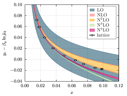
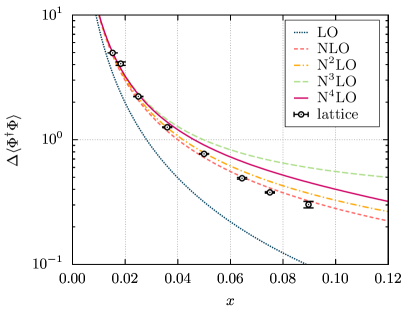
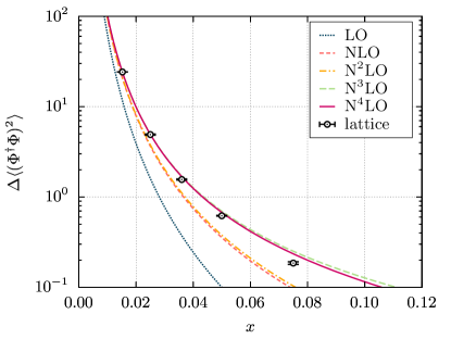
For the critical mass and the two condensates, we contrast our perturbative results with lattice simulations [31, 87, 88, 89, 69] in figs. 2 and 3. All three quantities display a marked improvement at small $x$; this is especially poignant for $\Delta\bigl{\langle}(\Phi^{\dagger}\Phi)^{2}\bigr{\rangle}$. As a consequence, the departure of perturbation theory from lattice data is delayed until $x\sim 0.04-0.05$. A subsequent breakdown of perturbation theory is indeed expected as a second-order transition takes place at $x=x_{*}=0.0983(13)$ [87, 88].

To illustrate the perturbative uncertainty at each order, we varied the renormalization scale in fig. 2, in the range $\bar{\mu}_{3}/(2m_{\mbox{\tiny\rm{$A$}}})=[10^{-\frac{1}{2}},10^{\frac{1}{2}}]$. An optimized value for $\bar{\mu}_{3}$ can be found à la principle of minimal sensitivity [90, 91, 50].

IV Impact on gravitational waves

To investigate the importance of three-loop corrections, we apply the results of sec. III to a four-dimensional parent theory that maps into eq. (1) in the high-temperature limit. For maximal freedom of the analysis, we treat our setup as a toy model for gravitational waves from a purely dark sector [92], and do not assume the Standard Model field content. To this end, we assume a ${\rm SU}(2)$ gauge theory with a scalar doublet $\Phi$ and an additional scalar singlet $S$. The model definition and its mapping into the thermal EFT are detailed in appendix C.

Pressure ($p$).

To derive the relevant equilibrium thermodynamic quantities for GW production, we construct the pressure in the high-temperature expansion. It is composed as

$\displaystyle p=p_{0}-TV_{\rm eff}\,,$ (43)

where $V_{\rm eff}$ is the effective potential of the 3D EFT computed in sec. II, separately for different phases. The unit operator $p_{0}$, or the field-independent pressure [24], comes from thermal corrections to the vacuum. From the pressure, we can find the enthalpy $\omega\equiv Tp^{\prime}$, the speed of sound $c_{s}^{2}\equiv p^{\prime}/e^{\prime}$, and the energy density $e=Tp^{\prime}-p$, where we use the shorthand $p^{\prime}\equiv{\rm d}p/{\rm d}T$.

To keep the discussion simple, we regroup the different perturbative orders of the pressure as “1-loop”, “2-loop”, and “3-loop”. A detailed composition of different perturbative orders of the pressure is given in appendix C.6.

We consider two scenarios for the dark-sector model:

  • (A)

    If the singlet is weakly coupled to a light doublet, the doublet can undergo a first-order phase transition while the singlet decouples.

  • (B)

    Even if the doublet is too heavy to accommodate a phase transition, a transition can be catalyzed if the interaction with the singlet is sufficiently strong. Here, we will work in a mass regime that admits integrating out the singlet such that only the doublet remains in the EFT.

By focusing on option (A), we fix the parameters of the parent theory (defined in appendix C.1) to

$\displaystyle g^{2}$ $\displaystyle=0.5\,,$ $\displaystyle\lambda_{\phi}$ $\displaystyle=0.0075\,,$ $\displaystyle M_{\phi}$ $\displaystyle=10\sqrt{2}\,,$ (BM-A)

(in arbitrary units of mass) and assume a simple tree-level relation $\mu^{2}_{\phi}=-M^{2}_{\phi}/2$ between the doublet mass parameter and the pole mass. The ratio $\lambda_{\phi}/g^{2}=0.015$ is the leading, temperature-independent contribution to the dimensionless variable $x$ that controls the behaviour of the EFT.

Refer to caption
Refer to caption
Figure 4: Pressure (top) and phase-transition strength (bottom) as function of temperature $T$ (scaled by scalar mass $M_{\phi}$) in a benchmark point (BM-A). From left to right, vertical lines indicate the nucleation temperatures and critical temperatures of tab. 1.

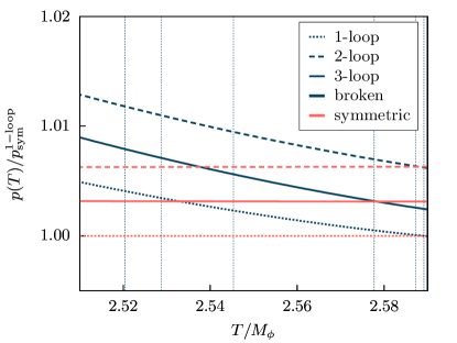
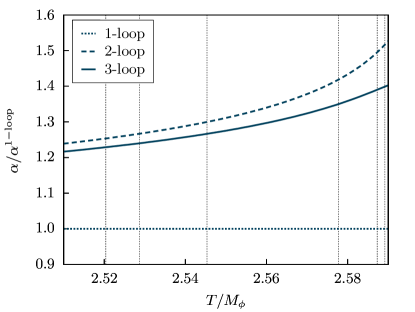
We illustrate the pressure as a function of temperature in fig. 4 (top) and normalize the pressure in both phases by the one-loop symmetric-phase pressure. Two-loop corrections affect the pressure at the 1% level, and subsequent three-loop corrections affect the pressure at at the 0.1% level, indicating excellent convergence.

Critical temperature ($T_{\rm c}$).

$T_{\rm c}$
1-loop 2.589
2-loop 2.587
3-loop 2.578
$T_{\rm p}$
LO 2.545
NLO 2.529
N${}^{2}$LO 2.520
Table 1: The critical temperature $T_{\rm c}$ and percolation temperature $T_{\rm p}$ in units of the scalar mass $M_{\phi}$ for benchmark point (BM-A) at different perturbative orders.

The critical temperature $T_{\rm c}$, at each order, corresponds to the temperatures where the pressure-difference of the phases vanishes. For (BM-A) the critical temperatures are listed in tab. 1 and depicted by the three rightmost vertical lines of fig 4. Since the broken-phase pressure has the symmetric-phase pressure subtracted, the pressure vanishes exactly at the critical mass $y_{\rm c}(x_{\rm c})$ at each order.333For determining $T_{\rm c}$, we employ the mixed method of [71]. Therein, only the effective potential is expanded in strict perturbation theory. For $T_{\rm c}$, we do not perform a strict expansion directly since a similar fully strict expansion for the phase transition strength, $\alpha$, would become a functionally formidable task.

In the temperature window of fig. 4, the critical $x_{\rm c}\approx 0.021$, as contributions of temporal scalars slightly increase the value of $x$ from its leading value set by $\lambda_{\phi}/g^{2}=0.015$; see appendix C. Since also $T^{2}/M^{2}_{\phi}\sim 6$, the high-temperature expansion is applicable.

We have verified that points with smaller (larger) $\lambda_{\phi}/g^{2}$ lead to increased (decreased) convergence in perturbation theory. Benchmark point (BM-A) illustrates such generic trends.

Phase transition strength ($\alpha$).

The convergence of the pressure is inherited by all quantities further derived from it. One such quantity is the phase transition strength defined via [93, 94]

$\displaystyle\alpha$ $\displaystyle=\frac{\Delta\bar{\theta}}{3\omega_{\mbox{\scriptsize sym}}}=\frac{1}{3p_{\mbox{\scriptsize sym}}^{\prime}}\Big{(}\frac{\Delta V_{\rm eff}}{c^{2}_{s,{\mbox{\scriptsize bro}}}}-\Delta\frac{{\rm d}V_{\rm eff}}{{\rm d}\ln T}\Big{)}\,,$ (44)

where the pseudotrace anomaly is $\bar{\theta}\equiv e-p/c^{2}_{s,{\mbox{\scriptsize bro}}}$ and where we used the notation $\Delta p\equiv p\bigl{|}_{\text{bro}}-p\bigl{|}_{\text{sym}}=-T\Delta V_{\rm eff}$.

In fig. 4 (bottom), we depict the relative-to-leading-order convergence of $\alpha$, in analogy to fig. 4 (top). For the pressure, the relative difference between different loop orders are minute due to the dominating unit operator $p_{0}$. Since $\alpha$ depends on the pressure difference, it is independent of $p_{0}$. Conversely, for $\alpha$, relative differences between one- and two-loop level can reach 10%, while the difference between two- and three-loop level displays great convergence.

Speed of sound ($c_{s}$).

While $\alpha$ is dominated by the second, derivative, term in eq. (44), the term proportional to $\Delta V_{\rm eff}$ is subdominant. This term also depends on the broken-phase speed of sound which is plotted in fig. 5.

Refer to caption
Refer to caption
Figure 5: As fig. 4 but depicting the speed of sound squared, $c_{s}^{2}$, as a function of temperature for the symmetric (top) and broken (bottom) phase.

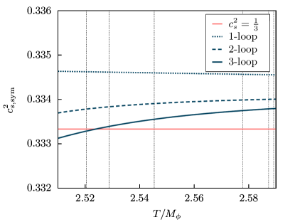
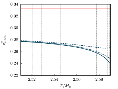
The symmetric-phase result is very close to the LO result $c_{s}^{2}=1/3$ at all orders. The broken-phase speed of sound significantly deviates from this LO value but quickly converges with the loop order. Such deviations can be important for analyses of hydrodynamic properties of the phase transition as they could affect the shape of the GW signal and suppress it by an order of magnitude [94, 93]. A careful computation of the speed of sound is required especially for theories whose particle content deviates strongly from the Standard Model one [95]. The article at hand completes the perturbative determination of the speed of sound.

Bubble nucleation rate ($\Gamma$).

Both figs. 4 and  5 depict the results for the bubble nucleation temperature, given by the three leftmost vertical lines from tab. 1. These results are obtained by directly following [96, 97]; see also [98, 27, 99, 100, 101, 102]. Here, we merely summarize the rationale for completeness. The bubble nucleation rate can be approximated by $\Gamma\simeq\frac{\kappa}{2\pi}\Sigma$, where the dynamical prefactor $\kappa$ depends on dissipative processes [103]. Its statistical part $\Sigma$ can be computed within the 3D EFT as

$\displaystyle\Sigma\approx[\mbox{det}_{S}]e^{-S_{B}(x,y)}\,,$ (45)

where $S_{B}$ is the bounce action and higher-order corrections are described by the determinant $[\mbox{det}_{S}]$. Henceforth, we simply work in approximations that ignore the dynamical prefactor $\kappa$ [104].

In the 3D EFT, $\Sigma$ depends only on $x,y$ and we can formally write the statistical part of the rate as an exponential $\exp(-S_{B}+\ln[\mbox{det}_{S}])\equiv\exp(-S_{\text{eff}})$, and further find the effective action in a strict expansion

$\displaystyle S_{\mbox{\scriptsize eff}}=S_{\mbox{\tiny\rm{LO}}}+xS_{\mbox{\tiny\rm{NLO}}}+x^{\frac{3}{2}}S_{\mbox{\tiny\rm{NNLO}}}+\ldots\,.$ (46)

Here, the powers of $x$ merely indicate the suppression relative to LO. Expressions for each order can be found in [97]. In analogy with sec. II, integer powers of $x$ come from integrating out vector bosons (in the UV), while fractional powers come from scalar fluctuations (in the IR).

To relate the statistical $S_{\mbox{\scriptsize eff}}$ to cosmology and the temperature evolution of the universe, we can approximate the condition for successful percolation after bubble nucleation as

$$S_{\mbox{\scriptsize eff}}(x,y_{\rm p})\simeq F[H(T_{\rm p})]\,,$$ (47)

where $F$ is a function of the Hubble parameter $H(T)$. The exact form of $F$ can be found in [105, 69, 106], but here we approximate it as a constant $F[H(T_{\rm p})]\approx 126$, which corresponds to about two-thirds of the universe being in the broken phase [106]. We remark that several definitions of $T_{\rm p}$ appear in the literature [10, 107, 11], and subtleties concerning this reference temperature for GW production were recently discussed in [108].

Given $S_{\mbox{\scriptsize eff}}(x,y_{\rm p})\equiv 126$, we can (numerically) find $y_{\rm p}(x)$ as a curve in the $(x,y)$-plane. For any parameter point of a parent theory, the percolation temperature $T_{\rm p}$ is given by the condition $y(x(T_{\rm p}))=y_{\rm p}(x)$.444 As [69], we employ $y_{\rm p}$ which is the “nucleation mass” $y_{\rm n}$ of [97]. This is analogous to finding the critical temperature from the condition $y(x(T_{\rm c}))=y_{\rm c}(x)$ [31].

In perturbation theory, we can find the LO result from $y(x(T_{\rm p}^{\mbox{\tiny\rm{LO}}}))=y_{\rm p}^{{\mbox{\tiny\rm{LO}}}}(x)$ where $y_{\rm p}^{{\mbox{\tiny\rm{LO}}}}$ is determined by $S_{\mbox{\tiny\rm{LO}}}$. The higher-order corrections $T_{\rm p}^{\mbox{\tiny\rm{NLO}}}$ and $T_{\rm p}^{\mbox{\tiny\rm{N${}^{2}$LO}}}$ are then found in a strict perturbative expansion, as detailed in [97]. In figs. 4 and 5, we observe that in (BM-A), the percolation and critical temperatures are rather close. This is a generic feature of this EFT where percolation occurs with relatively little supercooling below the critical temperature.

While for the critical temperature, we found all results including corrections up to and including N${}^{4}$LO, the strict expansion for the percolation temperature is performed only for the first three orders. The two remaining orders for the bubble nucleation rate are promoted to future work.

Inverse duration ($\beta/H$).

Another important thermal parameter for GW production is the inverse duration of the transition, defined as

$\displaystyle\frac{\beta}{H}$ $\displaystyle=-\frac{{\rm d}\ln\Gamma}{{\rm d}\ln T}\,.$ (48)

For the benchmark point (BM-A) of figs. 4 and 5, we report the values listed in tab. 2 for the phase transition strength, $\alpha$, and the inverse duration $\frac{\beta}{H}$ at $T=T_{\rm p}$.555 For $\frac{\beta}{H_{\rm p}}$, we determine the first three orders in strict perturbative expansion as described in [97].

$\alpha^{{\mbox{\tiny\rm{1-loop}}}}\bigl{(}T_{\rm p}^{\mbox{\tiny\rm{LO}}}\bigr{)}$ $\left(\frac{\beta}{H_{\rm p}}\right)_{{\mbox{\tiny\rm{LO${}_{\vphantom{x}}$}}}}$ 0.014
$\alpha^{{\mbox{\tiny\rm{2-loop}}}}\bigl{(}T_{\rm p}^{\mbox{\tiny\rm{NLO}}}\bigr{)}$ $\left(\frac{\beta}{H_{\rm p}}\right)_{{\mbox{\tiny\rm{NLO${}_{\vphantom{x}}$}}}}$ 0.020
$\alpha^{{\mbox{\tiny\rm{3-loop}}}}\bigl{(}T_{\rm p}^{\mbox{\tiny\rm{N${}^{2}$LO}}}\bigr{)}$ $\left(\frac{\beta}{H_{\rm p}}\right)_{{\mbox{\tiny\rm{N${}^{2}$LO${}_{\vphantom{x}}$}}}}$ 0.021
$\left(\frac{\beta}{H_{\rm p}}\right)_{{\mbox{\tiny\rm{LO${}_{\vphantom{x}}$}}}}$ 13578
$\left(\frac{\beta}{H_{\rm p}}\right)_{{\mbox{\tiny\rm{NLO${}_{\vphantom{x}}$}}}}$ 7182
$\left(\frac{\beta}{H_{\rm p}}\right)_{{\mbox{\tiny\rm{N${}^{2}$LO${}_{\vphantom{x}}$}}}}$ 4329
Table 2: The phase transition strength, $\alpha$, and inverse duration $\frac{\beta}{H_{\rm p}}$ for the benchmark point (BM-A) of figs. 4 and  5. Percolation temperatures correspond to tab. 1.

Higher-order corrections increase $\alpha$ and the overall convergence is good, while they decrease $\frac{\beta}{H_{\rm p}}$ and convergence is less pronounced, even for the relatively small value of $x\approx 0.021$ of (BM-A). The underlying perturbative computation of the bubble nucleation rate breaks down for $x>0.058$. We have verified improved convergence for parameter points that map into smaller values of $x$. Furthermore, we have verified that the aforementioned trends for $\alpha$ and $\frac{\beta}{H_{\rm p}}$ also hold for other parameter points.

Gravitational waves.

After detailing several phase transition thermodynamic quantities over a range of temperatures, we now emulate a scan over the model parameter space, typically performed in studies of cosmological phase transitions in beyond the Standard Model theories or dark sectors; cf. [10] and references therein. Along the lines of [10], we recast our scan results in the $(\alpha,\beta/H)$-plane in fig. 6 for the benchmark point (BM-A), varying $\lambda_{\phi}\in[0.001,0.03]$ which corresponds to $x\in[0.006,0.068]$ within the EFT. For illustration, we show tentative sensitivity regions of LISA and DECIGO in analogy with [109].666For connecting with LISA-generation experimental probes [110], we henceforth assume the scalar mass $M_{\phi}$ and all other dimensionful quantities in units of GeV. The tentative integrated sensitivity regions at a wall velocity $v_{w}=0.95$ for LISA at ${\rm SNR}=5$ [111] with $\mathcal{T}=4$ year mission duration [10] and DECIGO with the Correlation design [14] were taken from [109].

Refer to caption
Figure 6: Connecting our thermal computation to experimental probes via the $(\alpha_{\rm p},\beta/H_{\rm p})$-plane by projecting results for benchmark points (BM-A) but by varying $\lambda_{\phi}\in[0.0001,0.03]$ ($x\in[0.0054,0.068]$) and (IV) by varying $\lambda_{m}\in[2,2.55]$ ($x\in[0.017,0.098]$). Also shown are the tentative sensitivity regions for LISA [10] and DECIGO [14]. For these curves, $x$ decreases from left to right. For large $x$, the perturbative expansion for the bubble nucleation rate breaks down, resulting in tails of rapidly falling $\beta/H_{\rm p}$.

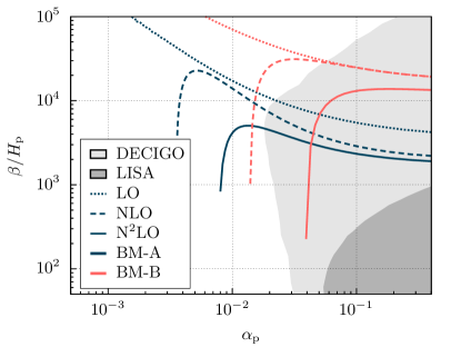
While none of the transitions have sufficiently large timescales for LISA to probe them,777 This result is expected since phase transitions that map into he 3D EFT of ${\rm SU}(2)$ with a doublet are not observable by LISA [48]. DECIGO and other future GW observatories could observe a primordial GW echo from a dark sector phase transition such as those analyzed here.

Parameter points with small $\lambda_{\phi}$ result in small $x$, which provide the largest (smallest) value for $\alpha_{\rm p}$ ($\beta/H_{\rm p}$) towards the bottom right. Even for the smallest values of $x$, perturbative corrections to $\beta/H_{\rm p}$ are sizeable. When $x$ increases, the perturbative computation for the inverse duration breaks completely, as indicated by the deviation of different orders towards the top left. Encouragingly, perturbation theory behaves best towards and within the DECIGO sensitivity, and a total breakdown of perturbation theory occurs only for weaker transitions, which is to be expected.

In fig. 6 and in addition to the benchmark point (BM-A) (blue), we also report on another benchmark point (IV) (red), viz.

$\displaystyle g^{2}$ $\displaystyle=0.9\,,$ $\displaystyle\lambda_{s}$ $\displaystyle=1.0\,,$ $\displaystyle\!\sin\theta$ $\displaystyle=0.2\,,$
$\displaystyle\frac{M_{\phi}}{\rm GeV}$ $\displaystyle=125\,,$ $\displaystyle\frac{M_{s}}{\rm GeV}$ $\displaystyle=325\,,$ $\displaystyle\!\frac{v_{0}}{\rm GeV}$ $\displaystyle=246\,,$ (BM-B)

where parameters are defined in appendix C.1. This scenario emulates the Standard Model augmented with a new scalar field. By design, the singlet is sufficiently heavy to be integrated out from the final EFT; see appendix C. This serves as an illuminating example that the 3D EFT of ${\rm SU}(2)$ with a doublet is an invaluable tool for studying the thermodynamics of electroweak-like first-order phase transitions in the presence of field content beyond the dynamical degrees of freedom of the final EFT [32, 37, 112, 113, 114, 115, 48].

V Discussion

This study delivers the final verdict of perturbation theory on electroweak gauge-Higgs theories at high temperature. By accounting for three-loop contributions, any further study perforce requires non-perturbative analyses due to the Linde problem. This article builds upon the recent formulation of the re-reorganized perturbative expansion [70]. While [70] computed its first three orders, here we deliver the remaining two perturbative orders and herald the culmination of a three-decade program initiated by [116, 68] for the perturbative analysis of cosmological and electroweak phase transitions in particular.

A similar perturbative completion was previously only achieved for pure scalar theory and QCD at high temperatures. For both theories, perturbative results are in remarkable agreement with non-perturbative lattice Monte-Carlo analyses [50, 62]. In turn, for electroweak gauge-Higgs theories, we find remarkable agreement between perturbation theory and lattice simulations by reorganizing the perturbative expansion. This provides additional evidence that the Linde problem is of minor significance in cosmological phase transitions driven by a fundamental scalar field.

Naturally, the precision of our perturbative results diminishes as we approach the critical point. At this juncture, the transition becomes second-order and subsequently evolves into a crossover. Perturbation theory is inherently unreliable for such weak transitions. One estimate suggests that perturbation theory can be trusted for positive critical masses, $y_{\rm c}$. However, once $y_{\rm c}$ turns negative, a second-order transition is expected within perturbation theory.

The perturbative toolbox completed in this article readily generalizes to more complicated theories with multiple scalar fields [71]. Thus, computing large perturbative higher-order corrections can follow the methodology outlined in this article. In particular, by utilizing the general mass hierarchy between the broken-phase vector bosons and the light transitioning scalar(s), we reorganized the theory to all perturbative orders.

For predictions of a stochastic GW background from a dark sector phase transition, we found that higher-order perturbative corrections ensure a well-controlled perturbation theory for equilibrium thermodynamics. However, the remaining significant uncertainty stems from the current inability to determine the bubble nucleation rate with similar precision. The extension of our findings to more complicated and widely studied theories with non-minimal scalar sectors, and their implications for collider phenomenology and GW predictions, is left to future studies.

Outlook.

With the perturbative program now completed, there is ample opportunity for future lattice studies. While perturbation theory can reliably predict the properties of strong transitions, it falls short in describing weak transitions where non-perturbative effects are large. To reliably rule out the possibility of a first-order transition, non-perturbative lattice analyses are essential. These analyses are particularly important for the phenomenological study of extensions of the Standard Model [51] and understanding their potential signatures at future colliders [117]. To this end, not only deciding the phase-transition character with lattice techniques is important, also future simulations for bubble nucleation [98, 118, 69, 104] and Sphaleron rates [119, 120, 121] are required.

To further enhance precision in understanding cosmological phase transitions, we consider the following future directions:

  • \SetWidth1.0\SetScale0.7 \DashLine(0,15)(22.5,15)3\DashLine(22.5 60 cos 22.5 mul add,15 60 sin 22.5 mul add)(22.5,15)3\DashLine(22.5 120 cos 22.5 mul add,15 120 sin 22.5 mul add)(22.5,15)3\DashLine(45,15)(22.5,15)3\DashLine(22.5 240 cos 22.5 mul add,15 240 sin 22.5 mul add)(22.5,15)3\DashLine(22.5 300 cos 22.5 mul add,15 300 sin 22.5 mul add)(22.5,15)3\Vertex(22.5,15)3

    At $\mathcal{O}(g^{6})$, additional contributions arise in the dimensional reduction via higher-dimensional operators within the 3D EFT. While evaluated for the pure gauge sector of QCD [122], accurately determining their effect in generic theories remains important for probing the validity of the 3D EFT. This validity forms a backbone not only for perturbative, but also lattice studies.

  • \SetWidth1.0\SetScale0.7 \CArc(15,15)(15,-60,60)\CArc(15,15)(15,60,120)\CArc(15,15)(15,120,240)\CArc(15,15)(15,240,300)\Line(15 60 cos 15 mul add,15 60 sin 15 mul add)(15 60 cos 15 mul add,15)\Line(15 60 cos 15 mul add,15)(15 60 cos 15 mul add,15 60 sin 15 mul sub)\Line(15 120 cos 15 mul add,15 120 sin 15 mul add)(15 120 cos 15 mul add,15)\Line(15 120 cos 15 mul add,15)(15 120 cos 15 mul add,15 120 sin 15 mul sub)\Line(15 120 cos 15 mul add,15)(15 60 cos 15 mul add,15)

    Purely perturbative $\mathcal{O}(g^{6})$ contributions from the hard scale could still be computed for the symmetric-phase pressure; cf. progress in hot QCD [123].

  • \SetWidth1.0\SetScale0.7 \CArc(10,15)(10,0,360)\CArc(50,15)(10,-180,180)\Line(20,15)(40,15)

    Building on [97, 124], the final perturbative corrections for the thermal bubble nucleation rate and the phase transition duration are yet to be computed. They still source one of the largest uncertainties for predicting GW signals from cosmological phase transitions.

Acknowledgements.
We are grateful to Oliver Gould, Joonas Hirvonen, Maciej Kierkla, Johan Löfgren, Lauri Niemi, Daniel Schmitt, Bogumiλa Świeżewska, Van Que Tran, Jorinde van de Vis, Yanda Wu and Guotao Xia for discussions as this project was carried out. The work of AE has been supported by the Swedish Research Council, project number VR:$2021$-$00363$. PS acknowledges support by the Deutsche Forschungsgemeinschaft (DFG, German Research Foundation) through the CRC-TR 211 ‘Strong-interaction matter under extreme conditions’ – project number 315477589 – TRR 211. PS acknowledges the hospitality of CERN during the final stages of this work. TT was supported under National Natural Science Foundation of China grant 12375094.

Appendix A Expansion of broken phase effective potential in terms of EFT matching

This appendix illustrates the organization of the perturbative series of fig. II for the broken-phase effective potential, in terms of an EFT matching between the mass scale of the vector bosons and the scale of the phase transition. By adopting the terminology of [71], these scales are dubbed soft and supersoft.

The supersoft scale EFT is constructed by integrating out the soft scale. The resulting action is

$\displaystyle S_{{\mbox{\scriptsize supersoft}}}^{{\mbox{\scriptsize tree}}}$ =𝐱12(is)2Zs+\SetWidth1.0\SetScale0.7 \Vertex(22.5,15)3 +\SetWidth1.0\SetScale0.7 \PhotonArc(15,15)(15,0,180)1 2 pi mul 15 mul 360 div 0 180 sub 0 180 sub mul sqrt mul Ldensity mul 2 div \PhotonArc(15,15)(15,180,360)1 2 pi mul 15 mul 360 div 180 360 sub 180 360 sub mul sqrt mul Ldensity mul 2 div LOfragments𝐱12(𝑖s)2Z𝑠fragments\SetWidth1.0\SetScale0.7 \Vertex(22.5,15)3 \SetWidth1.0\SetScale0.7 \PhotonArc(15,15)(15,0,180)1 2 pi mul 15 mul 360 div 0 180 sub 0 180 sub mul sqrt mul Ldensity mul 2 div \PhotonArc(15,15)(15,180,360)1 2 pi mul 15 mul 360 div 180 360 sub 180 360 sub mul sqrt mul Ldensity mul 2 div LO\displaystyle=\int_{{\bf x}}\frac{1}{2}(\partial_{i}s)^{2}Z_{s}+\underbrace{\;\parbox[c]{31.5pt}{\begin{picture}(31.5,21.0)(0.0,0.0)\SetWidth{1.0}\SetScale{0.7} \Vertex(22.5,15){3} \end{picture}}\;+\;\parbox[c]{21.0pt}{\begin{picture}(21.0,21.0)(0.0,0.0)\SetWidth{1.0}\SetScale{0.7} \PhotonArc(15,15)(15,0,180){1} {2 pi mul 15 mul 360 div 0 180 sub 0 180 sub mul sqrt mul Ldensity mul 2 div} \PhotonArc(15,15)(15,180,360){1} {2 pi mul 15 mul 360 div 180 360 sub 180 360 sub mul sqrt mul Ldensity mul 2 div} \end{picture}}\;}_{\text{LO}}
+\SetWidth1.0\SetScale0.7 \PhotonArc(15,15)(15,0,180)1 2 pi mul 15 mul 360 div 0 180 sub 0 180 sub mul sqrt mul Ldensity mul 2 div \PhotonArc(15,15)(15,180,360)1 2 pi mul 15 mul 360 div 180 360 sub 180 360 sub mul sqrt mul Ldensity mul 2 div \Photon(30,15)(0,15)1 30 0 sub 30 0 sub mul 15 15 sub 15 15 sub mul add sqrt Ldensity mul 2 div \SetWidth1.0\SetScale0.7 \PhotonArc(15,15)(15,0,360)1 2 pi mul 15 mul 360 div 0 360 sub 0 360 sub mul sqrt mul Ldensity mul 2 div \PhotonArc(45,15)(15,-180,180)1 2 pi mul 15 mul 360 div -180 180 sub -180 180 sub mul sqrt mul Ldensity mul 2 div \SetWidth1.0\SetScale0.7 \PhotonArc(15,15)(15,0,180)1 2 pi mul 15 mul 360 div 0 180 sub 0 180 sub mul sqrt mul Ldensity mul 2 div \PhotonArc(15,15)(15,180,360)1 2 pi mul 15 mul 360 div 180 360 sub 180 360 sub mul sqrt mul Ldensity mul 2 div\DashLine(30,15)(0,15)3 \SetWidth1.0\SetScale0.7 \DashCArc(15,15)(15,0,180)3\DashCArc(15,15)(15,180,360)3 \Photon(30,15)(0,15)1 30 0 sub 30 0 sub mul 15 15 sub 15 15 sub mul add sqrt Ldensity mul 2 div NLOfragmentsfragments\SetWidth1.0\SetScale0.7 \PhotonArc(15,15)(15,0,180)1 2 pi mul 15 mul 360 div 0 180 sub 0 180 sub mul sqrt mul Ldensity mul 2 div \PhotonArc(15,15)(15,180,360)1 2 pi mul 15 mul 360 div 180 360 sub 180 360 sub mul sqrt mul Ldensity mul 2 div \Photon(30,15)(0,15)1 30 0 sub 30 0 sub mul 15 15 sub 15 15 sub mul add sqrt Ldensity mul 2 div \SetWidth1.0\SetScale0.7 \PhotonArc(15,15)(15,0,360)1 2 pi mul 15 mul 360 div 0 360 sub 0 360 sub mul sqrt mul Ldensity mul 2 div \PhotonArc(45,15)(15,-180,180)1 2 pi mul 15 mul 360 div -180 180 sub -180 180 sub mul sqrt mul Ldensity mul 2 div \SetWidth1.0\SetScale0.7 \PhotonArc(15,15)(15,0,180)1 2 pi mul 15 mul 360 div 0 180 sub 0 180 sub mul sqrt mul Ldensity mul 2 div \PhotonArc(15,15)(15,180,360)1 2 pi mul 15 mul 360 div 180 360 sub 180 360 sub mul sqrt mul Ldensity mul 2 div\DashLine(30,15)(0,15)3 \SetWidth1.0\SetScale0.7 \DashCArc(15,15)(15,0,180)3\DashCArc(15,15)(15,180,360)3 \Photon(30,15)(0,15)1 30 0 sub 30 0 sub mul 15 15 sub 15 15 sub mul add sqrt Ldensity mul 2 div NLO\displaystyle+\underbrace{\;\parbox[c]{21.0pt}{\begin{picture}(21.0,21.0)(0.0,0.0)\SetWidth{1.0}\SetScale{0.7} \PhotonArc(15,15)(15,0,180){1} {2 pi mul 15 mul 360 div 0 180 sub 0 180 sub mul sqrt mul Ldensity mul 2 div} \PhotonArc(15,15)(15,180,360){1} {2 pi mul 15 mul 360 div 180 360 sub 180 360 sub mul sqrt mul Ldensity mul 2 div} \Photon(30,15)(0,15){1} {30 0 sub 30 0 sub mul 15 15 sub 15 15 sub mul add sqrt Ldensity mul 2 div} \end{picture}}\;\;\parbox[c]{42.0pt}{\begin{picture}(42.0,21.0)(0.0,0.0)\SetWidth{1.0}\SetScale{0.7} \PhotonArc(15,15)(15,0,360){1} {2 pi mul 15 mul 360 div 0 360 sub 0 360 sub mul sqrt mul Ldensity mul 2 div} \PhotonArc(45,15)(15,-180,180){1} {2 pi mul 15 mul 360 div -180 180 sub -180 180 sub mul sqrt mul Ldensity mul 2 div} \end{picture}}\;\;\parbox[c]{21.0pt}{\begin{picture}(21.0,21.0)(0.0,0.0)\SetWidth{1.0}\SetScale{0.7} \PhotonArc(15,15)(15,0,180){1} {2 pi mul 15 mul 360 div 0 180 sub 0 180 sub mul sqrt mul Ldensity mul 2 div} \PhotonArc(15,15)(15,180,360){1} {2 pi mul 15 mul 360 div 180 360 sub 180 360 sub mul sqrt mul Ldensity mul 2 div}\DashLine(30,15)(0,15){3} \end{picture}}\;\;\parbox[c]{21.0pt}{\begin{picture}(21.0,21.0)(0.0,0.0)\SetWidth{1.0}\SetScale{0.7} \DashCArc(15,15)(15,0,180){3}\DashCArc(15,15)(15,180,360){3} \Photon(30,15)(0,15){1} {30 0 sub 30 0 sub mul 15 15 sub 15 15 sub mul add sqrt Ldensity mul 2 div} \end{picture}}\;}_{\text{NLO}}
+\SetWidth1.0\SetScale0.7 \PhotonArc(15,15)(15,90,210)1 2 pi mul 15 mul 360 div 90 210 sub 90 210 sub mul sqrt mul Ldensity mul 2 div \PhotonArc(15,15)(15,210,330)1 2 pi mul 15 mul 360 div 210 330 sub 210 330 sub mul sqrt mul Ldensity mul 2 div \PhotonArc(15,15)(15,-30,90)1 2 pi mul 15 mul 360 div -30 90 sub -30 90 sub mul sqrt mul Ldensity mul 2 div \Photon(15,15)(15 15 90 cos mul add,15 15 90 sin mul add)1 15 15 15 90 cos mul add sub 15 15 15 90 cos mul add sub mul 15 15 15 90 sin mul add sub 15 15 15 90 sin mul add sub mul add sqrt Ldensity mul 2 div \Photon(15,15)(15 15 210 cos mul add,15 15 210 sin mul add)1 15 15 15 210 cos mul add sub 15 15 15 210 cos mul add sub mul 15 15 15 210 sin mul add sub 15 15 15 210 sin mul add sub mul add sqrt Ldensity mul 2 div \Photon(15,15)(15 15 330 cos mul add,15 15 330 sin mul add)1 15 15 15 330 cos mul add sub 15 15 15 330 cos mul add sub mul 15 15 15 330 sin mul add sub 15 15 15 330 sin mul add sub mul add sqrt Ldensity mul 2 div \SetWidth1.0\SetScale0.7 \PhotonArc(15,15)(15,0,180)1 2 pi mul 15 mul 360 div 0 180 sub 0 180 sub mul sqrt mul Ldensity mul 2 div \PhotonArc(15,15)(15,180,360)1 2 pi mul 15 mul 360 div 180 360 sub 180 360 sub mul sqrt mul Ldensity mul 2 div\DashLine(30,15)(15,15)3\DashLine(15,15)(0,15)3\GCirc(15,15)20 \SetWidth1.0\SetScale0.7 \DashCArc(15,15)(15,0,90)3\DashCArc(15,15)(15,90,180)3\DashCArc(15,15)(15,180,360)3 \Photon(30,15)(0,15)1 30 0 sub 30 0 sub mul 15 15 sub 15 15 sub mul add sqrt Ldensity mul 2 div\GCirc(15,30)20 N3LO,fragmentsfragments\SetWidth1.0\SetScale0.7 \PhotonArc(15,15)(15,90,210)1 2 pi mul 15 mul 360 div 90 210 sub 90 210 sub mul sqrt mul Ldensity mul 2 div \PhotonArc(15,15)(15,210,330)1 2 pi mul 15 mul 360 div 210 330 sub 210 330 sub mul sqrt mul Ldensity mul 2 div \PhotonArc(15,15)(15,-30,90)1 2 pi mul 15 mul 360 div -30 90 sub -30 90 sub mul sqrt mul Ldensity mul 2 div \Photon(15,15)(15 15 90 cos mul add,15 15 90 sin mul add)1 15 15 15 90 cos mul add sub 15 15 15 90 cos mul add sub mul 15 15 15 90 sin mul add sub 15 15 15 90 sin mul add sub mul add sqrt Ldensity mul 2 div \Photon(15,15)(15 15 210 cos mul add,15 15 210 sin mul add)1 15 15 15 210 cos mul add sub 15 15 15 210 cos mul add sub mul 15 15 15 210 sin mul add sub 15 15 15 210 sin mul add sub mul add sqrt Ldensity mul 2 div \Photon(15,15)(15 15 330 cos mul add,15 15 330 sin mul add)1 15 15 15 330 cos mul add sub 15 15 15 330 cos mul add sub mul 15 15 15 330 sin mul add sub 15 15 15 330 sin mul add sub mul add sqrt Ldensity mul 2 div \SetWidth1.0\SetScale0.7 \PhotonArc(15,15)(15,0,180)1 2 pi mul 15 mul 360 div 0 180 sub 0 180 sub mul sqrt mul Ldensity mul 2 div \PhotonArc(15,15)(15,180,360)1 2 pi mul 15 mul 360 div 180 360 sub 180 360 sub mul sqrt mul Ldensity mul 2 div\DashLine(30,15)(15,15)3\DashLine(15,15)(0,15)3\GCirc(15,15)20 \SetWidth1.0\SetScale0.7 \DashCArc(15,15)(15,0,90)3\DashCArc(15,15)(15,90,180)3\DashCArc(15,15)(15,180,360)3 \Photon(30,15)(0,15)1 30 0 sub 30 0 sub mul 15 15 sub 15 15 sub mul add sqrt Ldensity mul 2 div\GCirc(15,30)20 N3LO,\displaystyle+\underbrace{\;\parbox[c]{21.0pt}{\begin{picture}(21.0,21.0)(0.0,0.0)\SetWidth{1.0}\SetScale{0.7} \PhotonArc(15,15)(15,90,210){1} {2 pi mul 15 mul 360 div 90 210 sub 90 210 sub mul sqrt mul Ldensity mul 2 div} \PhotonArc(15,15)(15,210,330){1} {2 pi mul 15 mul 360 div 210 330 sub 210 330 sub mul sqrt mul Ldensity mul 2 div} \PhotonArc(15,15)(15,-30,90){1} {2 pi mul 15 mul 360 div -30 90 sub -30 90 sub mul sqrt mul Ldensity mul 2 div} \Photon(15,15)(15 15 90 cos mul add,15 15 90 sin mul add){1} {15 15 15 90 cos mul add sub 15 15 15 90 cos mul add sub mul 15 15 15 90 sin mul add sub 15 15 15 90 sin mul add sub mul add sqrt Ldensity mul 2 div} \Photon(15,15)(15 15 210 cos mul add,15 15 210 sin mul add){1} {15 15 15 210 cos mul add sub 15 15 15 210 cos mul add sub mul 15 15 15 210 sin mul add sub 15 15 15 210 sin mul add sub mul add sqrt Ldensity mul 2 div} \Photon(15,15)(15 15 330 cos mul add,15 15 330 sin mul add){1} {15 15 15 330 cos mul add sub 15 15 15 330 cos mul add sub mul 15 15 15 330 sin mul add sub 15 15 15 330 sin mul add sub mul add sqrt Ldensity mul 2 div} \end{picture}}\;\dots\;\parbox[c]{21.0pt}{\begin{picture}(21.0,21.0)(0.0,0.0)\SetWidth{1.0}\SetScale{0.7} \PhotonArc(15,15)(15,0,180){1} {2 pi mul 15 mul 360 div 0 180 sub 0 180 sub mul sqrt mul Ldensity mul 2 div} \PhotonArc(15,15)(15,180,360){1} {2 pi mul 15 mul 360 div 180 360 sub 180 360 sub mul sqrt mul Ldensity mul 2 div}\DashLine(30,15)(15,15){3}\DashLine(15,15)(0,15){3}\GCirc(15,15){2}{0} \end{picture}}\;\;\parbox[c]{21.0pt}{\begin{picture}(21.0,21.0)(0.0,0.0)\SetWidth{1.0}\SetScale{0.7} \DashCArc(15,15)(15,0,90){3}\DashCArc(15,15)(15,90,180){3}\DashCArc(15,15)(15,180,360){3} \Photon(30,15)(0,15){1} {30 0 sub 30 0 sub mul 15 15 sub 15 15 sub mul add sqrt Ldensity mul 2 div}\GCirc(15,30){2}{0} \end{picture}}\;}_{\text{N${}^{3}$LO}}\,, (49)

where the summation over the $s$ soft scalar fields is implied. The construction of the EFT action follows a standard EFT matching computation using the background-field method [78, 79, 80]; see also [125] for an intuitive explanation. In this framework, the strategy is to integrate only over soft, UV, momenta and expand the propagators in supersoft, IR, scalar masses before integration.

Hence, scalar propagators are treated as massless and their mass effect is included as a perturbative two-point interaction, presented as a blob at N${}^{4}$LO in eq. (A). These two-point interaction vertices appear at two-loop level, and are effectively counted as three-loop diagrams. The field normalization factor $Z_{s}$, resulting from the soft gauge field modes, is computed at one-loop order; see e.g. [100]. Pure scalar-field diagrams vanish in dimensional regularization given that no scales appear in the propagators. They do not contribute to the matching. However, scalar-field loops are computed within the supersoft EFT in the IR, and at one-loop order are

Ssupersoft1-loopfragmentsSsupersoft1-loop\displaystyle S_{{\mbox{\scriptsize supersoft}}}^{{\mbox{\scriptsize 1-loop}}} =\SetWidth1.0\SetScale0.7 \DashCArc(15,15)(15,0,180)3\DashCArc(15,15)(15,180,360)3 N2LO+\SetWidth1.0\SetScale0.7 \DashCArc(15,15)(15,-90,270)3\GCirc(15,0)20   \SetWidth1.0\SetScale0.7 \DashCArc(15,15)(15,-90,270)3\FBoxc(15,0)(5,5)   N4LO,fragmentsfragments\SetWidth1.0\SetScale0.7 \DashCArc(15,15)(15,0,180)3\DashCArc(15,15)(15,180,360)3 N2LOfragments\SetWidth1.0\SetScale0.7 \DashCArc(15,15)(15,-90,270)3\GCirc(15,0)20   \SetWidth1.0\SetScale0.7 \DashCArc(15,15)(15,-90,270)3\FBoxc(15,0)(5,5)   N4LO,\displaystyle=\underbrace{\;\parbox[c]{21.0pt}{\begin{picture}(21.0,21.0)(0.0,0.0)\SetWidth{1.0}\SetScale{0.7} \DashCArc(15,15)(15,0,180){3}\DashCArc(15,15)(15,180,360){3} \end{picture}}\;}_{\text{N${}^{2}$LO}}+\underbrace{\;\;\parbox[c]{21.0pt}{\begin{picture}(21.0,21.0)(0.0,0.0)\SetWidth{1.0}\SetScale{0.7} \DashCArc(15,15)(15,-90,270){3}\GCirc(15,0){2}{0} \; \end{picture}}\;\;\;\parbox[c]{21.0pt}{\begin{picture}(21.0,21.0)(0.0,0.0)\SetWidth{1.0}\SetScale{0.7} \DashCArc(15,15)(15,-90,270){3}\FBoxc(15,0)(5,5) \; \end{picture}}\;}_{\text{N${}^{4}$LO}}\,, (50)

where the “$x$-expansion” is enforced by treating higher-order contributions (in powers of $x$) to the scalar mass as perturbative corrections. These corrections are denoted by a blob insertion of $\Pi_{\phi}$; see eq. (18). A box denotes the insertion of the two-point vertex $\bar{\Pi}_{\phi}$ arising from field renormalization; see eq. (21). Two-loop diagrams within the supersoft EFT are of higher order than N${}^{4}$LO and can thus be omitted in our computation. Combining the results for the soft expansion of eq. (A) and the supersoft corrections in eq. (50), yields the perturbative expansion of the broken-phase effective potential in fig. II.

Appendix B
Thermodynamics of U(1) + Higgs theory

The three-dimensional theory action of the Abelian Higgs model is given by eq. (1) and its tree-level potential by eq. (2) where the scalar $\Phi$ transforms under ${\rm U}(1)$. This model has previously been studied in [126, 127, 128, 129, 130, 131]. Contrary to the ${\rm SU}(2)$ model, there is no magnetic mass for the photon. Thus making four-loop computations tractable; at least in principle. However, a non-perturbative mass exists for finite lattice spacings [132, 133], and topological effects such as vortices are relevant [134, 135, 136]. In the context of ${\rm SU}(2)$ + adjoint Higgs theory, similar effects were recently discussed in [137].

For the symmetric phase, the first two orders $V_{\rm eff}\bigr{|}_{{\mbox{\tiny\rm{LO}}}}^{{\mbox{\scriptsize sym}}}=V_{\rm eff}\bigr{|}_{{\mbox{\tiny\rm{NLO}}}}^{{\mbox{\scriptsize sym}}}\equiv 0$. The first non-vanishing contributions arise at N${}^{3}$LO and N${}^{4}$LO,

$\displaystyle V_{\rm eff}\bigr{|}_{{\mbox{\tiny\rm{N${}^{2}$LO}}}}^{{\mbox{\scriptsize sym}}}$ $\displaystyle=-\frac{1}{6\pi}\bigl{(}m_{3}^{2}\bigr{)}^{\frac{3}{2}}\,,$ (51)
$\displaystyle V_{\rm eff}\bigr{|}_{{\mbox{\tiny\rm{N${}^{3}$LO}}}}^{{\mbox{\scriptsize sym}}}$ $\displaystyle=-\frac{g_{3}^{2}m_{3}^{2}}{(4\pi)^{2}}\frac{1}{2}\Bigl{[}-3+4\ln 2+2\ln\frac{m_{3}^{2}}{\bar{\mu}_{3}^{2}}\Bigr{]}\,,$ (52)
$\displaystyle V_{\rm eff}\bigr{|}_{{\mbox{\tiny\rm{N${}^{4}$LO}}}}^{{\mbox{\scriptsize sym}}}$ $\displaystyle=\frac{g_{3}^{4}}{(4\pi)^{3}}\frac{\bigl{(}m_{3}^{2}\bigr{)}^{\frac{1}{2}}}{12}\Bigl{[}97+4\pi^{2}$
$\displaystyle\hphantom{\frac{g_{3}^{4}}{(4\pi)^{3}}\frac{\bigl{(}m_{3}^{2}\bigr{)}^{\frac{1}{2}}}{12}\Bigl{[}}-136\ln 2-24\ln\frac{m_{3}^{2}}{\bar{\mu}_{3}^{2}}\Bigr{]}\,.$ (53)

The broken-phase effective potential amounts to

$\displaystyle V_{\rm eff}\bigr{|}_{{\mbox{\tiny\rm{LO}}}}^{{\mbox{\scriptsize bro}}}$ $\displaystyle=\frac{1}{2}m_{3}^{2}\phi^{2}+\frac{1}{4}\lambda_{3}\phi^{4}-\frac{1}{6\pi}g_{3}^{3}\phi^{3}\,,$ (54)
$\displaystyle V_{\rm eff}\bigr{|}_{{\mbox{\tiny\rm{NLO}}}}^{{\mbox{\scriptsize bro}}}$ $\displaystyle=\frac{g_{3}^{4}\phi^{2}}{(4\pi)^{2}}\Bigl{[}-1-2\ln\frac{\bar{\mu}_{3}}{2g_{3}\phi}\Bigl{]}\,,$ (55)
$\displaystyle V_{\rm eff}\bigr{|}_{{\mbox{\tiny\rm{N${}^{2}$LO}}}}^{{\mbox{\scriptsize bro}}}$ $\displaystyle=-\frac{1}{12\pi}\Bigl{[}\widetilde{m}_{h}^{3}+\widetilde{m}_{{\mbox{\tiny\rm{$G$}}}}^{3}\Bigl{]}\,,$ (56)
$\displaystyle V_{\rm eff}\bigr{|}_{{\mbox{\tiny\rm{N${}^{3}$LO}}}}^{{\mbox{\scriptsize bro}}}$ $\displaystyle=\frac{4g_{3}^{2}}{(16\pi)^{2}}\Bigl{[}m_{3}^{2}\Bigl{(}3+4\ln 2+8\ln\frac{\bar{\mu}_{3}}{2g_{3}\phi}\Bigr{)}$
$\displaystyle\hphantom{\frac{4g_{3}^{2}}{(16\pi)^{2}}}+\lambda_{3}\phi^{2}\Bigl{(}7+4\ln 2+16\ln\frac{\bar{\mu}_{3}}{2g_{3}\phi}\Bigr{)}\Bigr{]}$
$\displaystyle+\frac{g_{3}^{5}\phi}{(16\pi)^{3}}\frac{16}{3}\Bigl{[}77+4\pi^{2}-104\ln 2\Bigr{]}\,,$ (57)
$\displaystyle V_{\rm eff}\bigr{|}_{{\mbox{\tiny\rm{N${}^{4}$LO}}}}^{{\mbox{\scriptsize bro}}}$ $\displaystyle=-\frac{g_{3}}{(16\pi)^{2}}\frac{1}{\phi}\frac{4}{3}\Bigl{[}11\widetilde{m}_{h}^{3}+16\widetilde{m}_{{\mbox{\tiny\rm{$G$}}}}^{3}\Bigr{]}$
$\displaystyle+\frac{2g_{3}^{4}}{(4\pi)^{3}}\Bigl{[}-\widetilde{m}_{h}+(\widetilde{m}_{h}+\widetilde{m}_{{\mbox{\tiny\rm{$G$}}}})\ln\frac{\bar{\mu}_{3}}{2g_{3}\phi}\Bigr{]}\,.$ (58)

The perturbative results of the critical mass and condensates for this model up to N${}^{2}$LO, are

$\displaystyle y_{\rm c}$ $\displaystyle=\frac{1}{2(3\pi)^{2}x}\Bigl{[}1+\frac{9}{2}x\ln\tilde{\mu}_{3}-\Bigl{(}\frac{x}{2}\Bigr{)}^{\frac{3}{2}}\Bigr{]}\,,$ (59)
$\displaystyle\Delta\bigl{\langle}\Phi^{\dagger}\Phi\bigr{\rangle}_{\mbox{\scriptsize c}}$ $\displaystyle=\frac{1}{2(3\pi)^{2}x^{2}}\Bigl{[}1-\frac{9}{2}x+\frac{25}{2}\Bigl{(}\frac{x}{2}\Bigr{)}^{\frac{3}{2}}\Bigr{]}\,,$ (60)
$\displaystyle\Delta\bigl{\langle}\left(\Phi^{\dagger}\Phi\right)^{2}\bigr{\rangle}_{\mbox{\scriptsize c}}$ $\displaystyle=\frac{1}{2^{2}(3\pi)^{4}x^{4}}\Bigl{[}1-9x+13\Bigl{(}\frac{x}{2}\Bigr{)}^{\frac{3}{2}}\Bigr{]}\,,$ (61)

where $\tilde{\mu}_{3}\equiv e^{\tfrac{1}{2}+\ln\tfrac{3}{2}}(\pi x\bar{\mu}_{3})$. After including three-loop corrections, we find the critical mass and condensates at N${}^{3}$LO and N${}^{4}$LO to be

$\displaystyle y_{\rm c}\bigr{|}_{{\mbox{\tiny\rm{N${}^{3}$LO}}}}$ $\displaystyle=-\frac{x^{2}}{{2^{3}(4\pi)^{2}x}}\biggl{[}64\ln\bigl{(}x^{\frac{9}{8}}\bar{\mu}_{3}\pi\bigr{)}+63+4\pi^{2}-152\ln 2+64\ln 3\biggr{]}\,,$ (62)
$\displaystyle\Delta\bigl{\langle}\Phi^{\dagger}\Phi\bigr{\rangle}_{\mbox{\scriptsize c}}\bigr{|}_{{\mbox{\tiny\rm{N${}^{3}$LO}}}}$ $\displaystyle=\frac{x^{2}}{{2^{3}(4\pi)^{2}x^{2}}}\biggl{[}24\ln x+111+4\pi^{2}-104\ln 2\biggr{]}\,,$ (63)
$\displaystyle\Delta\bigl{\langle}\bigl{(}\Phi^{\dagger}\Phi\bigr{)}^{2}\bigr{\rangle}_{\mbox{\scriptsize c}}\bigr{|}_{{\mbox{\tiny\rm{N${}^{3}$LO}}}}$ $\displaystyle=\frac{x^{2}}{{2^{6}(3\pi)^{4}x^{4}}}\biggl{[}216\ln x+\frac{1755}{2}+18\pi^{2}-576\ln 2+144\ln(3\pi)\biggr{]}\,,$ (64)
$\displaystyle y_{\rm c}\bigr{|}_{{\mbox{\tiny\rm{N${}^{4}$LO}}}}$ $\displaystyle=-\frac{x^{\frac{5}{2}}}{{2^{\frac{5}{2}}(4\pi)^{2}x}}\Bigl{[}12\ln x-\frac{85}{6}-2\pi^{2}+32\ln 2\Bigr{]}\,,$ (65)
$\displaystyle\Delta\bigl{\langle}\Phi^{\dagger}\Phi\bigr{\rangle}_{\mbox{\scriptsize c}}\bigr{|}_{{\mbox{\tiny\rm{N${}^{4}$LO}}}}$ $\displaystyle=\frac{x^{\frac{5}{2}}}{{2^{\frac{7}{2}}(4\pi)^{2}x^{2}}}\Bigl{[}60\ln x-\frac{143}{2}-10\pi^{2}+160\ln 2\Bigr{]}\,,$ (66)
$\displaystyle\Delta\bigl{\langle}\bigl{(}\Phi^{\dagger}\Phi\bigr{)}^{2}\bigr{\rangle}_{\mbox{\scriptsize c}}\bigr{|}_{{\mbox{\tiny\rm{N${}^{4}$LO}}}}$ $\displaystyle=\frac{x^{\frac{5}{2}}}{{2^{\frac{9}{2}}(3\pi)^{4}x^{4}}}\Bigl{[}54\ln x-\frac{1341}{8}-9\pi^{2}+144\ln 2\Bigr{]}\,.$ (67)

Appendix C Thermal EFT for SU(2) with a doublet and singlet dark sector

This appendix details the model employed in sec. IV. While most of the results can be extracted from the literature [26, 112, 38, 39, 95], we include and display novel thermal corrections.

C.1 Model at zero temperature

We define our setup through the Lagrangian

$\displaystyle\mathcal{L}=\frac{1}{4}F_{\mu\nu}^{a}F_{\mu\nu}^{a}$ $\displaystyle+(D_{\mu}\Phi)^{\dagger}(D_{\mu}\Phi)$
$\displaystyle+\frac{1}{2}(\partial_{\mu}S)^{2}+V(\Phi,S)\,,$ (68)

where the covariant derivative $D_{\mu}\Phi=(\partial_{\mu}-igA_{\mu})\Phi$, where $A_{\mu}=A_{\mu}^{a}T^{a}$. The scalar potential is

$\displaystyle V(\Phi,S)$ $\displaystyle=m^{2}_{\phi}\Phi^{\dagger}\Phi+\lambda_{\phi}(\Phi^{\dagger}\Phi)^{2}+\frac{1}{2}m_{s}^{2}S^{2}+\frac{1}{4}\lambda_{s}S^{4}$
$\displaystyle+\frac{1}{2}\mu_{m}(\Phi^{\dagger}\Phi)^{2}S+\frac{1}{2}\lambda_{m}(\Phi^{\dagger}\Phi)^{2}S^{2}$
$\displaystyle+\mu_{1}S+\frac{1}{3}\mu_{3}S^{3}\,.$ (69)

The cubic portal allows for doublet-singlet mixing. We work in a parametrization where the mixing angle $\sin\theta$, the scalar mass squared eigenvalues $M^{2}_{\phi}$, $M^{2}_{s}$,888 For a small mixing angle $\sin\theta\ll 1$, the mass $M_{\phi}$ describes the mostly doublet and $M_{s}$ the mostly singlet state. the doublet vacuum expectation value (VEV) at zero temperature $v_{0}$, the gauge coupling $g^{2}$, the singlet self interactions $\lambda_{s}$, $\mu_{3}$, and the portal coupling $\lambda_{m}$ are treated as input parameters. We fix the singlet VEV to vanish which fixes singlet tadpole coupling $\mu_{1}=-\mu_{m}v^{2}_{0}/4$. Concretely, we use the tree-level relations

$\displaystyle m^{2}_{\phi}$ $\displaystyle=-\frac{1}{4}\Big{(}M^{2}_{\phi}+M^{2}_{s}+(M^{2}_{\phi}-M^{2}_{s})\cos(2\theta)\Big{)}\,,$
$\displaystyle m^{2}_{s}$ $\displaystyle=\frac{1}{2}\Big{(}-\lambda_{m}v^{2}_{0}+M^{2}_{\phi}+M^{2}_{s}-(M^{2}_{\phi}-M^{2}_{s})\cos(2\theta)\Big{)}\,,$
$\displaystyle\lambda_{\phi}$ $\displaystyle=\frac{1}{4v^{2}_{0}}\Big{(}M^{2}_{\phi}+M^{2}_{s}+(M^{2}_{\phi}-M^{2}_{s})\cos(2\theta)\Big{)}\,,$
$\displaystyle\mu_{m}$ $\displaystyle=-\frac{2}{v_{0}}(M^{2}_{\phi}-M^{2}_{s})\sin\theta\cos\theta\,.$ (70)

For a realistic theory, instead of a dark-sector toy setup, it would be warranted to improve these relations by the corresponding zero-temperature one-loop corrections [26], cf. [39].

C.2 Effective theory

At high temperatures $m^{2}_{\phi}/T,m^{2}_{s}/T\sim g\ll 1$ and the 3D zero Matsubara modes live in the IR at the soft scale $|p|\sim\mathcal{O}(gT)$. In turn, the non-zero Matsubara modes in the UV at scale $|p|\sim\mathcal{O}(\pi T)$ can be integrated out [138]. The resulting 3D EFT is of the same functional form as eq. (C.1) with the addition of the Lagrangian for the temporal component of the gauge field

$\displaystyle\mathcal{L}^{{\mbox{\tiny\rm{3d}}}}_{\mbox{\scriptsize temporal}}$ $\displaystyle=\frac{1}{2}(D_{r}A^{a}_{0})^{2}+\frac{1}{2}m_{\mbox{\tiny\rm{D}}}^{2}\,A^{a}_{0}A^{a}_{0}$
$\displaystyle+\frac{1}{4}\kappa_{3}\,(A^{a}_{0}A^{a}_{0})^{2}+\frac{1}{2}h_{3}\,\phi^{\dagger}\phi A^{a}_{0}A^{a}_{0}$
$\displaystyle+\frac{1}{4}y_{3}\,S^{2}A^{a}_{0}A^{a}_{0}+\frac{1}{2}x_{3}\,S^{2}A^{a}_{0}A^{a}_{0}\;,$ (71)

where the covariant derivative for triplet ${\rm SU}(2)$ temporal scalars, reads $D_{r}A_{0}^{a}=\partial_{r}A^{a}_{0}+g_{3}\epsilon^{abc}A^{b}_{r}A^{c}_{0}$. Here, we chose different normalizations for $h_{3}$ [26, 11], $y_{3}$, and $x_{3}$ compared to [38]. In addition, $\kappa_{3}\equiv 2\text{\tt$\lambda$VLL[1]}$ compared to the convention used by DRalgo; see the dark-su2-higgs-singlet.m model file [139].

In analogy to eq. (A), the construction of the EFT can be schematically illustrated in terms of the effective action as

SEFT[φ]=𝐱12(iφ)2Zφ+\SetWidth1.0\SetScale0.7 \Vertex(22.5,15)3 +\SetWidth1.0\SetScale0.7 \CArc(15,15)(15,0,180)\CArc(15,15)(15,180,360) +\SetWidth1.0\SetScale0.7 \CArc(15,15)(15,0,180)\CArc(15,15)(15,180,360)\Line(30,15)(0,15) fragmentsSEFT[φ]𝐱12(𝑖φ)2Z𝜑\SetWidth1.0\SetScale0.7 \Vertex(22.5,15)3 \SetWidth1.0\SetScale0.7 \CArc(15,15)(15,0,180)\CArc(15,15)(15,180,360) \SetWidth1.0\SetScale0.7 \CArc(15,15)(15,0,180)\CArc(15,15)(15,180,360)\Line(30,15)(0,15) \displaystyle S_{{\mbox{\tiny\rm{EFT}}}}[\varphi]=\int_{{\bf x}}\frac{1}{2}(\partial_{i}\varphi)^{2}Z_{\varphi}+\;\parbox[c]{31.5pt}{\begin{picture}(31.5,21.0)(0.0,0.0)\SetWidth{1.0}\SetScale{0.7} \Vertex(22.5,15){3} \end{picture}}\;+\;\parbox[c]{21.0pt}{\begin{picture}(21.0,21.0)(0.0,0.0)\SetWidth{1.0}\SetScale{0.7} \CArc(15,15)(15,0,180)\CArc(15,15)(15,180,360) \end{picture}}\;+\;\parbox[c]{21.0pt}{\begin{picture}(21.0,21.0)(0.0,0.0)\SetWidth{1.0}\SetScale{0.7} \CArc(15,15)(15,0,180)\CArc(15,15)(15,180,360)\Line(30,15)(0,15) \end{picture}}\;
=𝐱{p0φ=0+[\SetWidth1.0\SetScale0.7 \DashLine(0,15)(22.5,15)3 \FilledPolygon( 0 22.5 0 sub 3 div add 4 15 15 sub 22.5 0 sub atan 45 add cos mul add, 15 15 15 sub 3 div add 4 15 15 sub 22.5 0 sub atan 45 add sin mul add)( 0 22.5 0 sub 3 div add 4 15 15 sub 22.5 0 sub atan 135 add cos mul add, 15 15 15 sub 3 div add 4 15 15 sub 22.5 0 sub atan 135 add sin mul add)( 0 22.5 0 sub 3 div add 4 15 15 sub 22.5 0 sub atan 225 add cos mul add, 15 15 15 sub 3 div add 4 15 15 sub 22.5 0 sub atan 225 add sin mul add)( 0 22.5 0 sub 3 div add 4 15 15 sub 22.5 0 sub atan 315 add cos mul add, 15 15 15 sub 3 div add 4 15 15 sub 22.5 0 sub atan 315 add sin mul add)black \DashLine(45,15)(22.5,15)3\Vertex(22.5,15)3 +\SetWidth1.0\SetScale0.7 \DashLine(0,15)(15.5,15)3 \FilledPolygon( 0 15.5 0 sub 3 div add 4 15 15 sub 15.5 0 sub atan 45 add cos mul add, 15 15 15 sub 3 div add 4 15 15 sub 15.5 0 sub atan 45 add sin mul add)( 0 15.5 0 sub 3 div add 4 15 15 sub 15.5 0 sub atan 135 add cos mul add, 15 15 15 sub 3 div add 4 15 15 sub 15.5 0 sub atan 135 add sin mul add)( 0 15.5 0 sub 3 div add 4 15 15 sub 15.5 0 sub atan 225 add cos mul add, 15 15 15 sub 3 div add 4 15 15 sub 15.5 0 sub atan 225 add sin mul add)( 0 15.5 0 sub 3 div add 4 15 15 sub 15.5 0 sub atan 315 add cos mul add, 15 15 15 sub 3 div add 4 15 15 sub 15.5 0 sub atan 315 add sin mul add)black \DashLine(30.5,15)(45,15)3\GCirc(22.5,15)80.75 \Text(22.5,15)[c]1+\SetWidth1.0\SetScale0.7 \DashLine(0,15)(15.5,15)3\DashLine(30.5,15)(45,15)3\GCirc(22.5,15)80.75 \Text(22.5,15)[c]2fragments𝐱{p0fragmentsφ0[\SetWidth1.0\SetScale0.7 \DashLine(0,15)(22.5,15)3 \FilledPolygon( 0 22.5 0 sub 3 div add 4 15 15 sub 22.5 0 sub atan 45 add cos mul add, 15 15 15 sub 3 div add 4 15 15 sub 22.5 0 sub atan 45 add sin mul add)( 0 22.5 0 sub 3 div add 4 15 15 sub 22.5 0 sub atan 135 add cos mul add, 15 15 15 sub 3 div add 4 15 15 sub 22.5 0 sub atan 135 add sin mul add)( 0 22.5 0 sub 3 div add 4 15 15 sub 22.5 0 sub atan 225 add cos mul add, 15 15 15 sub 3 div add 4 15 15 sub 22.5 0 sub atan 225 add sin mul add)( 0 22.5 0 sub 3 div add 4 15 15 sub 22.5 0 sub atan 315 add cos mul add, 15 15 15 sub 3 div add 4 15 15 sub 22.5 0 sub atan 315 add sin mul add)black \DashLine(45,15)(22.5,15)3\Vertex(22.5,15)3 \SetWidth1.0\SetScale0.7 \DashLine(0,15)(15.5,15)3 \FilledPolygon( 0 15.5 0 sub 3 div add 4 15 15 sub 15.5 0 sub atan 45 add cos mul add, 15 15 15 sub 3 div add 4 15 15 sub 15.5 0 sub atan 45 add sin mul add)( 0 15.5 0 sub 3 div add 4 15 15 sub 15.5 0 sub atan 135 add cos mul add, 15 15 15 sub 3 div add 4 15 15 sub 15.5 0 sub atan 135 add sin mul add)( 0 15.5 0 sub 3 div add 4 15 15 sub 15.5 0 sub atan 225 add cos mul add, 15 15 15 sub 3 div add 4 15 15 sub 15.5 0 sub atan 225 add sin mul add)( 0 15.5 0 sub 3 div add 4 15 15 sub 15.5 0 sub atan 315 add cos mul add, 15 15 15 sub 3 div add 4 15 15 sub 15.5 0 sub atan 315 add sin mul add)black \DashLine(30.5,15)(45,15)3\GCirc(22.5,15)80.75 \Text(22.5,15)[c]1\SetWidth1.0\SetScale0.7 \DashLine(0,15)(15.5,15)3\DashLine(30.5,15)(45,15)3\GCirc(22.5,15)80.75 \Text(22.5,15)[c]2\displaystyle=\!\int_{{\bf x}}\bigg{\{}p_{0}^{\varphi=0}+\bigg{[}\;\parbox[c]{31.5pt}{\begin{picture}(31.5,21.0)(0.0,0.0)\SetWidth{1.0}\SetScale{0.7} \DashLine(0,15)(22.5,15){3} \FilledPolygon{( 0 22.5 0 sub 3 div add 4 15 15 sub 22.5 0 sub atan 45 add cos mul add, 15 15 15 sub 3 div add 4 15 15 sub 22.5 0 sub atan 45 add sin mul add)( 0 22.5 0 sub 3 div add 4 15 15 sub 22.5 0 sub atan 135 add cos mul add, 15 15 15 sub 3 div add 4 15 15 sub 22.5 0 sub atan 135 add sin mul add)( 0 22.5 0 sub 3 div add 4 15 15 sub 22.5 0 sub atan 225 add cos mul add, 15 15 15 sub 3 div add 4 15 15 sub 22.5 0 sub atan 225 add sin mul add)( 0 22.5 0 sub 3 div add 4 15 15 sub 22.5 0 sub atan 315 add cos mul add, 15 15 15 sub 3 div add 4 15 15 sub 22.5 0 sub atan 315 add sin mul add)}{black} \DashLine(45,15)(22.5,15){3}\Vertex(22.5,15){3} \end{picture}}\;+\;\parbox[c]{31.5pt}{\begin{picture}(31.5,21.0)(0.0,0.0)\SetWidth{1.0}\SetScale{0.7} \DashLine(0,15)(15.5,15){3} \FilledPolygon{( 0 15.5 0 sub 3 div add 4 15 15 sub 15.5 0 sub atan 45 add cos mul add, 15 15 15 sub 3 div add 4 15 15 sub 15.5 0 sub atan 45 add sin mul add)( 0 15.5 0 sub 3 div add 4 15 15 sub 15.5 0 sub atan 135 add cos mul add, 15 15 15 sub 3 div add 4 15 15 sub 15.5 0 sub atan 135 add sin mul add)( 0 15.5 0 sub 3 div add 4 15 15 sub 15.5 0 sub atan 225 add cos mul add, 15 15 15 sub 3 div add 4 15 15 sub 15.5 0 sub atan 225 add sin mul add)( 0 15.5 0 sub 3 div add 4 15 15 sub 15.5 0 sub atan 315 add cos mul add, 15 15 15 sub 3 div add 4 15 15 sub 15.5 0 sub atan 315 add sin mul add)}{black} \DashLine(30.5,15)(45,15){3}\GCirc(22.5,15){8}{0.75} \Text(22.5,15)[c]{$\scriptstyle 1$} \end{picture}}\;+\;\parbox[c]{31.5pt}{\begin{picture}(31.5,21.0)(0.0,0.0)\SetWidth{1.0}\SetScale{0.7} \DashLine(0,15)(15.5,15){3}\DashLine(30.5,15)(45,15){3}\GCirc(22.5,15){8}{0.75} \Text(22.5,15)[c]{$\scriptstyle 2$} \end{picture}}\;
+[\SetWidth1.0\SetScale0.7 \DashLine(22.5 45 cos 22.5 mul add,15 45 sin 22.5 mul add)(22.5,15)3 \FilledPolygon( 22.5 45 cos 22.5 mul add 22.5 22.5 45 cos 22.5 mul add sub 3 div add 4 15 15 45 sin 22.5 mul add sub 22.5 22.5 45 cos 22.5 mul add sub atan 45 add cos mul add, 15 45 sin 22.5 mul add 15 15 45 sin 22.5 mul add sub 3 div add 4 15 15 45 sin 22.5 mul add sub 22.5 22.5 45 cos 22.5 mul add sub atan 45 add sin mul add)( 22.5 45 cos 22.5 mul add 22.5 22.5 45 cos 22.5 mul add sub 3 div add 4 15 15 45 sin 22.5 mul add sub 22.5 22.5 45 cos 22.5 mul add sub atan 135 add cos mul add, 15 45 sin 22.5 mul add 15 15 45 sin 22.5 mul add sub 3 div add 4 15 15 45 sin 22.5 mul add sub 22.5 22.5 45 cos 22.5 mul add sub atan 135 add sin mul add)( 22.5 45 cos 22.5 mul add 22.5 22.5 45 cos 22.5 mul add sub 3 div add 4 15 15 45 sin 22.5 mul add sub 22.5 22.5 45 cos 22.5 mul add sub atan 225 add cos mul add, 15 45 sin 22.5 mul add 15 15 45 sin 22.5 mul add sub 3 div add 4 15 15 45 sin 22.5 mul add sub 22.5 22.5 45 cos 22.5 mul add sub atan 225 add sin mul add)( 22.5 45 cos 22.5 mul add 22.5 22.5 45 cos 22.5 mul add sub 3 div add 4 15 15 45 sin 22.5 mul add sub 22.5 22.5 45 cos 22.5 mul add sub atan 315 add cos mul add, 15 45 sin 22.5 mul add 15 15 45 sin 22.5 mul add sub 3 div add 4 15 15 45 sin 22.5 mul add sub 22.5 22.5 45 cos 22.5 mul add sub atan 315 add sin mul add)black \DashLine(22.5 135 cos 22.5 mul add,15 135 sin 22.5 mul add)(22.5,15)3\DashLine(22.5 225 cos 22.5 mul add,15 225 sin 22.5 mul add)(22.5,15)3\DashLine(22.5 315 cos 22.5 mul add,15 315 sin 22.5 mul add)(22.5,15)3\Vertex(22.5,15)3 +\SetWidth1.0\SetScale0.7 \DashLine(22.5 45 cos 22.5 mul add,15 45 sin 22.5 mul add)(22.5,15)3\DashLine(22.5 135 cos 22.5 mul add,15 135 sin 22.5 mul add)(22.5,15)3\DashLine(22.5 225 cos 22.5 mul add,15 225 sin 22.5 mul add)(22.5,15)3\DashLine(22.5 315 cos 22.5 mul add,15 315 sin 22.5 mul add)(22.5,15)3\GCirc(22.5,15)80.75 \Text(22.5,15)[c]1]+[\SetWidth1.0\SetScale0.7 \DashLine(22.5 0 cos 22.5 mul add,15 0 sin 22.5 mul add)(22.5,15)3\DashLine(22.5 60 cos 22.5 mul add,15 60 sin 22.5 mul add)(22.5,15)3\DashLine(22.5 120 cos 22.5 mul add,15 120 sin 22.5 mul add)(22.5,15)3\DashLine(22.5 180 cos 22.5 mul add,15 180 sin 22.5 mul add)(22.5,15)3\DashLine(22.5 240 cos 22.5 mul add,15 240 sin 22.5 mul add)(22.5,15)3\DashLine(22.5 300 cos 22.5 mul add,15 300 sin 22.5 mul add)(22.5,15)3\GCirc(22.5,15)80.75 \Text(22.5,15)[c]1]}fragments[\SetWidth1.0\SetScale0.7 \DashLine(22.5 45 cos 22.5 mul add,15 45 sin 22.5 mul add)(22.5,15)3 \FilledPolygon( 22.5 45 cos 22.5 mul add 22.5 22.5 45 cos 22.5 mul add sub 3 div add 4 15 15 45 sin 22.5 mul add sub 22.5 22.5 45 cos 22.5 mul add sub atan 45 add cos mul add, 15 45 sin 22.5 mul add 15 15 45 sin 22.5 mul add sub 3 div add 4 15 15 45 sin 22.5 mul add sub 22.5 22.5 45 cos 22.5 mul add sub atan 45 add sin mul add)( 22.5 45 cos 22.5 mul add 22.5 22.5 45 cos 22.5 mul add sub 3 div add 4 15 15 45 sin 22.5 mul add sub 22.5 22.5 45 cos 22.5 mul add sub atan 135 add cos mul add, 15 45 sin 22.5 mul add 15 15 45 sin 22.5 mul add sub 3 div add 4 15 15 45 sin 22.5 mul add sub 22.5 22.5 45 cos 22.5 mul add sub atan 135 add sin mul add)( 22.5 45 cos 22.5 mul add 22.5 22.5 45 cos 22.5 mul add sub 3 div add 4 15 15 45 sin 22.5 mul add sub 22.5 22.5 45 cos 22.5 mul add sub atan 225 add cos mul add, 15 45 sin 22.5 mul add 15 15 45 sin 22.5 mul add sub 3 div add 4 15 15 45 sin 22.5 mul add sub 22.5 22.5 45 cos 22.5 mul add sub atan 225 add sin mul add)( 22.5 45 cos 22.5 mul add 22.5 22.5 45 cos 22.5 mul add sub 3 div add 4 15 15 45 sin 22.5 mul add sub 22.5 22.5 45 cos 22.5 mul add sub atan 315 add cos mul add, 15 45 sin 22.5 mul add 15 15 45 sin 22.5 mul add sub 3 div add 4 15 15 45 sin 22.5 mul add sub 22.5 22.5 45 cos 22.5 mul add sub atan 315 add sin mul add)black \DashLine(22.5 135 cos 22.5 mul add,15 135 sin 22.5 mul add)(22.5,15)3\DashLine(22.5 225 cos 22.5 mul add,15 225 sin 22.5 mul add)(22.5,15)3\DashLine(22.5 315 cos 22.5 mul add,15 315 sin 22.5 mul add)(22.5,15)3\Vertex(22.5,15)3 \SetWidth1.0\SetScale0.7 \DashLine(22.5 45 cos 22.5 mul add,15 45 sin 22.5 mul add)(22.5,15)3\DashLine(22.5 135 cos 22.5 mul add,15 135 sin 22.5 mul add)(22.5,15)3\DashLine(22.5 225 cos 22.5 mul add,15 225 sin 22.5 mul add)(22.5,15)3\DashLine(22.5 315 cos 22.5 mul add,15 315 sin 22.5 mul add)(22.5,15)3\GCirc(22.5,15)80.75 \Text(22.5,15)[c]1][\SetWidth1.0\SetScale0.7 \DashLine(22.5 0 cos 22.5 mul add,15 0 sin 22.5 mul add)(22.5,15)3\DashLine(22.5 60 cos 22.5 mul add,15 60 sin 22.5 mul add)(22.5,15)3\DashLine(22.5 120 cos 22.5 mul add,15 120 sin 22.5 mul add)(22.5,15)3\DashLine(22.5 180 cos 22.5 mul add,15 180 sin 22.5 mul add)(22.5,15)3\DashLine(22.5 240 cos 22.5 mul add,15 240 sin 22.5 mul add)(22.5,15)3\DashLine(22.5 300 cos 22.5 mul add,15 300 sin 22.5 mul add)(22.5,15)3\GCirc(22.5,15)80.75 \Text(22.5,15)[c]1]}\displaystyle\hphantom{{}=\int_{{\bf x}}\bigg{\{}p_{0}^{\varphi=0}}\!+\bigg{[}\;\parbox[c]{31.5pt}{\begin{picture}(31.5,21.0)(0.0,0.0)\SetWidth{1.0}\SetScale{0.7} \DashLine(22.5 45 cos 22.5 mul add,15 45 sin 22.5 mul add)(22.5,15){3} \FilledPolygon{( 22.5 45 cos 22.5 mul add 22.5 22.5 45 cos 22.5 mul add sub 3 div add 4 15 15 45 sin 22.5 mul add sub 22.5 22.5 45 cos 22.5 mul add sub atan 45 add cos mul add, 15 45 sin 22.5 mul add 15 15 45 sin 22.5 mul add sub 3 div add 4 15 15 45 sin 22.5 mul add sub 22.5 22.5 45 cos 22.5 mul add sub atan 45 add sin mul add)( 22.5 45 cos 22.5 mul add 22.5 22.5 45 cos 22.5 mul add sub 3 div add 4 15 15 45 sin 22.5 mul add sub 22.5 22.5 45 cos 22.5 mul add sub atan 135 add cos mul add, 15 45 sin 22.5 mul add 15 15 45 sin 22.5 mul add sub 3 div add 4 15 15 45 sin 22.5 mul add sub 22.5 22.5 45 cos 22.5 mul add sub atan 135 add sin mul add)( 22.5 45 cos 22.5 mul add 22.5 22.5 45 cos 22.5 mul add sub 3 div add 4 15 15 45 sin 22.5 mul add sub 22.5 22.5 45 cos 22.5 mul add sub atan 225 add cos mul add, 15 45 sin 22.5 mul add 15 15 45 sin 22.5 mul add sub 3 div add 4 15 15 45 sin 22.5 mul add sub 22.5 22.5 45 cos 22.5 mul add sub atan 225 add sin mul add)( 22.5 45 cos 22.5 mul add 22.5 22.5 45 cos 22.5 mul add sub 3 div add 4 15 15 45 sin 22.5 mul add sub 22.5 22.5 45 cos 22.5 mul add sub atan 315 add cos mul add, 15 45 sin 22.5 mul add 15 15 45 sin 22.5 mul add sub 3 div add 4 15 15 45 sin 22.5 mul add sub 22.5 22.5 45 cos 22.5 mul add sub atan 315 add sin mul add)}{black} \DashLine(22.5 135 cos 22.5 mul add,15 135 sin 22.5 mul add)(22.5,15){3}\DashLine(22.5 225 cos 22.5 mul add,15 225 sin 22.5 mul add)(22.5,15){3}\DashLine(22.5 315 cos 22.5 mul add,15 315 sin 22.5 mul add)(22.5,15){3}\Vertex(22.5,15){3} \end{picture}}\;+\;\parbox[c]{31.5pt}{\begin{picture}(31.5,21.0)(0.0,0.0)\SetWidth{1.0}\SetScale{0.7} \DashLine(22.5 45 cos 22.5 mul add,15 45 sin 22.5 mul add)(22.5,15){3}\DashLine(22.5 135 cos 22.5 mul add,15 135 sin 22.5 mul add)(22.5,15){3}\DashLine(22.5 225 cos 22.5 mul add,15 225 sin 22.5 mul add)(22.5,15){3}\DashLine(22.5 315 cos 22.5 mul add,15 315 sin 22.5 mul add)(22.5,15){3}\GCirc(22.5,15){8}{0.75} \Text(22.5,15)[c]{$\scriptstyle 1$} \end{picture}}\;\bigg{]}+\bigg{[}\;\parbox[c]{31.5pt}{\begin{picture}(31.5,21.0)(0.0,0.0)\SetWidth{1.0}\SetScale{0.7} \DashLine(22.5 0 cos 22.5 mul add,15 0 sin 22.5 mul add)(22.5,15){3}\DashLine(22.5 60 cos 22.5 mul add,15 60 sin 22.5 mul add)(22.5,15){3}\DashLine(22.5 120 cos 22.5 mul add,15 120 sin 22.5 mul add)(22.5,15){3}\DashLine(22.5 180 cos 22.5 mul add,15 180 sin 22.5 mul add)(22.5,15){3}\DashLine(22.5 240 cos 22.5 mul add,15 240 sin 22.5 mul add)(22.5,15){3}\DashLine(22.5 300 cos 22.5 mul add,15 300 sin 22.5 mul add)(22.5,15){3}\GCirc(22.5,15){8}{0.75} \Text(22.5,15)[c]{$\scriptstyle 1$} \end{picture}}\;\bigg{]}\bigg{\}}
$\displaystyle=\!\int_{{\bf x}}\bigg{\{}\underbrace{\!p_{0}^{\varphi=0}+\frac{1}{2}\varphi^{2}\big{(}m^{2}_{3}\big{)}+\frac{1}{4}\varphi^{4}\big{(}\lambda_{3}\big{)}}_{\mathcal{O}(g^{4})}+\mathcal{O}(g^{6}\varphi^{6})\bigg{\}}\,,$ (72)

where encircled numbers indicate the loop order and boxes indicate kinetic insertions on external lines in analogy with eq. (20). Here, the effective action is computed using the background field method, in terms of a formal scalar background field $\varphi$. For simplicity, we present here only one such background field, keeping in mind that for multiple scalar fields within the EFT, each field has its own background. Furthermore, in this simplified illustration, we do not detail the background field method for the gauge sector.

In the first line of eq. (C.2), loop diagrams involving Matsubara sum-integrals are integrated over the hard momenta, i.e. over non-zero Matsubara modes in the UV. Masses $M^{2}(\varphi)$ in propagators depend on the background field, and sum-integrals are computed in the high-temperature expansion of $M^{2}/T^{2}\sim g^{2}$. Matsubara zero modes in the IR are treated as massless. The field normalization factor

Zφ=1+ddk2[\SetWidth1.0\SetScale0.7 \DashLine(0,15)(7.5,15)3 \DashLine(37.5,15)(45,15)3 \CArc(22.5,15)(15,0,180)\CArc(22.5,15)(15,180,360) ],fragmentsZ𝜑1dfragmentsdk2[\SetWidth1.0\SetScale0.7 \DashLine(0,15)(7.5,15)3 \DashLine(37.5,15)(45,15)3 \CArc(22.5,15)(15,0,180)\CArc(22.5,15)(15,180,360) ],\displaystyle Z_{\varphi}=1+\frac{{\rm d}}{{\rm d}k^{2}}\biggl{[}\;\parbox[c]{31.5pt}{\begin{picture}(31.5,21.0)(0.0,0.0)\SetWidth{1.0}\SetScale{0.7} \DashLine(0,15)(7.5,15){3} \DashLine(37.5,15)(45,15){3} \CArc(22.5,15)(15,0,180)\CArc(22.5,15)(15,180,360) \end{picture}}\;\biggr{]}\,, (73)

is likewise obtained by integrating over non-zero Matsubara modes, and computing the relevant scalar two-point functions in an expansion of soft external momenta $k$.

In the second line of eq. (C.2), we have expanded the action in terms of background field, $\varphi$. We have highlighted that the unit operator $p_{0}$ is field-independent, and return to its computation below. Terms with non-vanishing background field correspond to Green’s functions generated by the effective action, and the ellipsis denotes eight- and higher-point correlators.

In the third line of eq. (C.2), we identify these Green’s functions with EFT parameters of the scalar potential, that we denote by a schematic $m^{2}_{3}$ and $\lambda_{3}$ for this simplified illustration. We remark, that in the second line, the effect of the $Z$-factor is captured by the Green’s functions999 $Z$-factor contributions are crucial to obtain a renormalization-scale invariant, gauge-independent result [11, 100]. which is illustrated by a box on the external lines. In practice, the 3D parameter matching relations can be determined by directly computing Green’s functions without the presence of the background field, instead of computing the action. This is practical, especially for the gauge, and gauge-scalar mixed sectors [26].

Assuming a power counting in which the parent theory squared mass parameters are soft $\sim(gT)^{2}$, in the high-$T$ expansion and the quartic couplings scale as $\mathcal{O}(g^{2})$, allows for determining all 3D EFT parameters at $\mathcal{O}(g^{4})$ provided that the masses are determined at two-loop and couplings at one-loop level. Sextic and higher operators can be neglected as they contribute at $\mathcal{O}(g^{6})$.

Within the so-far constructed EFT, the Debye mass $m_{\mbox{\tiny\rm{D}}}^{2}$ is soft, and parametrically larger than the mass of the scalar doublet $\Phi$ that undergoes the transition deeper in the IR. This allows to integrate out the temporal scalar $A^{a}_{0}$, to build an EFT at a softer scale. In addition, we assume that the singlet mass $m_{s}\sim m_{\mbox{\tiny\rm{D}}}$, and hence the singlet is integrated out as well. The resulting EFT in the IR is given by eq. (1).

Constructing this softer EFT aligns with eq. (C.2) with a few modifications. In this case, only the soft loops of the temporal scalar and the singlet are integrated over, while the doublet (as well as spatial gauge field) are treated as massless. The convergence of the soft theory is slower as each new loop order is suppressed by $g$, whereas in the hard-to-soft matching, the loop suppression is $g^{2}$. Typically, in softer theory only one-loop effects from the soft scale are included for the scalar quartic coupling [26]. While this is numerically an excellent approximation for contributions of the temporal scalar, for the singlet, also two-loop effects can be sizable. Similarly, effects from the soft singlet can induce sizable corrections to the sextic operator, to which soft contributions in general are parametrically $\mathcal{O}(g^{3})$ [26]. While at first glance this might seem alarming, we comment on these issues in sec. C.5 when we present concrete expressions and further discuss our numerical analysis.

The unit operator in the final EFT composes of $p_{0}=p_{{\mbox{\tiny\rm{E}}}}+p_{\mbox{\tiny\rm{M}}}$ [74], where hard and soft contributions, typically labelled as electrostatic ($p_{{\mbox{\tiny\rm{E}}}}$) and magnetic ($p_{{\mbox{\tiny\rm{M}}}}$), follow from vacuum diagrams of the form (here in four-dimensional units)

pE=\SetWidth1.0\SetScale0.7 \CArc(15,15)(15,0,180)\CArc(15,15)(15,180,360) fragmentspE\SetWidth1.0\SetScale0.7 \CArc(15,15)(15,0,180)\CArc(15,15)(15,180,360) \displaystyle p_{{\mbox{\tiny\rm{E}}}}=\;\parbox[c]{21.0pt}{\begin{picture}(21.0,21.0)(0.0,0.0)\SetWidth{1.0}\SetScale{0.7} \CArc(15,15)(15,0,180)\CArc(15,15)(15,180,360) \end{picture}}\; +\SetWidth1.0\SetScale0.7 \CArc(15,15)(15,0,180)\CArc(15,15)(15,180,360)\Line(30,15)(0,15) +\SetWidth1.0\SetScale0.7 \CArc(15,15)(15,90,210)\CArc(15,15)(15,210,330)\CArc(15,15)(15,-30,90)\Line(15,15)(15 15 90 cos mul add,15 15 90 sin mul add)\Line(15,15)(15 15 210 cos mul add,15 15 210 sin mul add)\Line(15,15)(15 15 330 cos mul add,15 15 330 sin mul add) fragments\SetWidth1.0\SetScale0.7 \CArc(15,15)(15,0,180)\CArc(15,15)(15,180,360)\Line(30,15)(0,15) \SetWidth1.0\SetScale0.7 \CArc(15,15)(15,90,210)\CArc(15,15)(15,210,330)\CArc(15,15)(15,-30,90)\Line(15,15)(15 15 90 cos mul add,15 15 90 sin mul add)\Line(15,15)(15 15 210 cos mul add,15 15 210 sin mul add)\Line(15,15)(15 15 330 cos mul add,15 15 330 sin mul add) \displaystyle+\;\parbox[c]{21.0pt}{\begin{picture}(21.0,21.0)(0.0,0.0)\SetWidth{1.0}\SetScale{0.7} \CArc(15,15)(15,0,180)\CArc(15,15)(15,180,360)\Line(30,15)(0,15) \end{picture}}\;+\;\parbox[c]{21.0pt}{\begin{picture}(21.0,21.0)(0.0,0.0)\SetWidth{1.0}\SetScale{0.7} \CArc(15,15)(15,90,210)\CArc(15,15)(15,210,330)\CArc(15,15)(15,-30,90)\Line(15,15)(15 15 90 cos mul add,15 15 90 sin mul add)\Line(15,15)(15 15 210 cos mul add,15 15 210 sin mul add)\Line(15,15)(15 15 330 cos mul add,15 15 330 sin mul add) \end{picture}}\;
$\displaystyle\sim T^{4}\Bigl{(}g^{0}+g^{2}+g^{4}+\mathcal{O}(g^{6})\Bigr{)}\,,$ (74)
pM=T(\SetWidth1.0\SetScale0.7 \DashCArc(15,15)(15,0,180)3\DashCArc(15,15)(15,180,360)3 fragmentspMT(\SetWidth1.0\SetScale0.7 \DashCArc(15,15)(15,0,180)3\DashCArc(15,15)(15,180,360)3 \displaystyle p_{{\mbox{\tiny\rm{M}}}}=T\Bigl{(}\;\parbox[c]{21.0pt}{\begin{picture}(21.0,21.0)(0.0,0.0)\SetWidth{1.0}\SetScale{0.7} \DashCArc(15,15)(15,0,180){3}\DashCArc(15,15)(15,180,360){3} \end{picture}}\; +\SetWidth1.0\SetScale0.7 \DashCArc(15,15)(15,0,180)3\DashCArc(15,15)(15,180,360)3\DashLine(30,15)(0,15)3 +\SetWidth1.0\SetScale0.7 \DashCArc(15,15)(15,90,210)3\DashCArc(15,15)(15,210,330)3\DashCArc(15,15)(15,-30,90)3\DashLine(15,15)(15 15 90 cos mul add,15 15 90 sin mul add)3\DashLine(15,15)(15 15 210 cos mul add,15 15 210 sin mul add)3\DashLine(15,15)(15 15 330 cos mul add,15 15 330 sin mul add)3 )fragments\SetWidth1.0\SetScale0.7 \DashCArc(15,15)(15,0,180)3\DashCArc(15,15)(15,180,360)3\DashLine(30,15)(0,15)3 \SetWidth1.0\SetScale0.7 \DashCArc(15,15)(15,90,210)3\DashCArc(15,15)(15,210,330)3\DashCArc(15,15)(15,-30,90)3\DashLine(15,15)(15 15 90 cos mul add,15 15 90 sin mul add)3\DashLine(15,15)(15 15 210 cos mul add,15 15 210 sin mul add)3\DashLine(15,15)(15 15 330 cos mul add,15 15 330 sin mul add)3 )\displaystyle+\;\parbox[c]{21.0pt}{\begin{picture}(21.0,21.0)(0.0,0.0)\SetWidth{1.0}\SetScale{0.7} \DashCArc(15,15)(15,0,180){3}\DashCArc(15,15)(15,180,360){3}\DashLine(30,15)(0,15){3} \end{picture}}\;+\;\parbox[c]{21.0pt}{\begin{picture}(21.0,21.0)(0.0,0.0)\SetWidth{1.0}\SetScale{0.7} \DashCArc(15,15)(15,90,210){3}\DashCArc(15,15)(15,210,330){3}\DashCArc(15,15)(15,-30,90){3}\DashLine(15,15)(15 15 90 cos mul add,15 15 90 sin mul add){3}\DashLine(15,15)(15 15 210 cos mul add,15 15 210 sin mul add){3}\DashLine(15,15)(15 15 330 cos mul add,15 15 330 sin mul add){3} \end{picture}}\;\Bigl{)}
$\displaystyle\sim T^{4}\Bigl{(}g^{3}+g^{4}+g^{5}+\mathcal{O}(g^{6})\Bigr{)}\,,$ (75)

where each loop order is represented by its most complicated topology.

For $p_{\mbox{\tiny\rm{E}}}$, the loop integration is over non-zero Matsubara modes and each order is suppressed by $g^{2}$. For $p_{\mbox{\tiny\rm{M}}}$, loops involve soft fields and each order is suppressed by $g$. In both cases, all contributions are purely perturbative and for hot QCD, the computation of the four-loop $\mathcal{O}(g^{6})$ has recently been organized at the level of master integrals [123].

C.3 Collection of expressions

This section collects all relevant thermal corrections for the softer EFT. Installing the power counting

$\displaystyle m^{2}_{\phi},m^{2}_{s}$ $\displaystyle\sim(gT)^{2}\,,$ $\displaystyle\lambda_{\phi},\lambda_{s},\lambda_{m}$ $\displaystyle\sim g^{2}\,,$
$\displaystyle\mu_{3},\mu_{m}$ $\displaystyle\sim g^{2}T\,,$ (76)

leads to a similar EFT construction as in [39], and the hard-to-soft matching relations can be read from therein (by omitting ${\rm U}(1)$, ${\rm SU}(3)$, and fermionic sectors contributions). Alternatively, one can compute the parameters using DRalgo [40] via the model file [139]. Hence, we do not list these relations here.

The matching results in the two-loop mass parameters (and singlet tadpole) and one-loop couplings. Such relations are renormalization-scale invariant at $\mathcal{O}(g^{4})$, and in our numerical analysis, we apply one-loop $\beta$-functions to run parameters to the optimal thermal scale $\bar{\mu}_{\mbox{\scriptsize opt}}=4\pi e^{-{\gamma_{\mbox{\tiny\rm{E}}}}}T$ [68], where ${\gamma_{\mbox{\tiny\rm{E}}}}$ is the Euler-Mascheroni constant. Since the required $\beta$-functions can be obtained with DRalgo, we do not list them explicitly.

If the singlet decouples, we need smaller doublet self-coupling which satisfies the parametric scaling $\lambda_{\phi}\sim g^{3}/\pi$; cf. (BM-A). Also in this case, we include $\mathcal{O}(\lambda^{2}_{\phi})$ terms in the hard-to-soft matching, yet remark that these contributions, as well as $\mathcal{O}(g^{2}\lambda_{\phi})$, are miniscule compared to pure gauge contributions of $\mathcal{O}(g^{4})$ that dominate.

In (IV), and by further fixing $\lambda_{m}=2.5$ in this section, we find that $\lambda_{\phi}$, $\lambda_{m}$, $\lambda_{s}$, and the gauge coupling contribute with approximately equal importance to the two-loop thermal mass parameters, while the effect from cubic couplings is less important.101010 Contributions of $\mu_{3}$, $\mu_{m}$ to one-loop thermal masses are $\propto L_{b}$ and vanish at the optimized $\bar{\mu}_{\mbox{\tiny\rm{opt}}}=4\pi e^{-{\gamma_{\mbox{\tiny\rm{E}}}}}T$. Further corrections to the matching relations from these couplings are $\propto\zeta_{3}/(4\pi)^{4}$ or $\zeta_{5}/(4\pi)^{6}$ and we find them to be negligible; cf. sec. 4.2 of [38]. Cubic couplings, however, yield the largest (one-loop) correction for the singlet tadpole which is dominated by its tree-level value while two-loop corrections are further suppressed. For both mass parameters, tree-level and one-loop contributions are dominant while the two-loop correction is subdominant. This indicates a controlled high-$T$ expansion, and concretely $m^{2}_{\phi}/T\sim 1/4$ and $m^{2}_{s}/T\sim 4/5$ in vicinity of critical temperature $T_{\rm c}\sim 188$ GeV.

The unit operator for the hard modes from eq. (C.2) and the soft modes from eq. (C.2), can be obtained with DRalgo and reads

$\displaystyle p_{{\mbox{\tiny\rm{E}}}}$ $\displaystyle=11\frac{\pi^{2}}{90}T^{4}-\frac{T^{2}}{576}\Big{(}T^{2}(39g^{2}+24\lambda_{\phi}+4\lambda_{m}+3\lambda_{s})+24(4m^{2}_{\phi}+m^{2}_{s})\Big{)}$
$\displaystyle+\frac{T^{2}}{(4\pi)^{2}}\Big{[}\frac{m^{2}_{s}}{24}L_{b}\Bigl{(}2\lambda_{m}+3\lambda_{s}\Bigr{)}+m^{2}_{\phi}\Big{(}L_{b}\Bigl{(}\lambda_{\phi}+\frac{1}{12}\lambda_{m}\Bigr{)}+\frac{g^{2}}{8}\Bigl{(}-2+12\ln(2\pi)-12(\ln\zeta_{2})^{\prime}+9L_{b}\Bigr{)}\Big{)}$
$\displaystyle\hphantom{{}\frac{T^{2}}{(4\pi)^{2}}\bigg{[}}-\frac{1}{48}\bigl{(}4\mu^{2}_{3}+3\mu^{2}_{m}\bigr{)}\bigl{(}2\ln(2\pi)-2(\ln\zeta_{2})^{\prime}+L_{b}\bigr{)}\Big{]}-\frac{L_{b}}{(4\pi)^{2}}\bigl{(}\mu^{4}_{\phi}+\frac{1}{4}\mu^{4}_{s}\bigr{)}$
$\displaystyle+\frac{T^{4}}{(4\pi)^{2}}\Big{[}\alpha_{{\mbox{\tiny\rm{E$g^{4}$}}}}g^{4}\!+\!\alpha_{{\mbox{\tiny\rm{E$\lambda_{\phi}g^{2}$}}}}\lambda_{\phi}g^{2}\!+\alpha_{{\mbox{\tiny\rm{E$\lambda^{2}_{\phi}$}}}}\lambda_{\phi}^{2}\!+\alpha_{{\mbox{\tiny\rm{E$\lambda_{m}g^{2}$}}}}\lambda_{m}g^{2}\!+\alpha_{{\mbox{\tiny\rm{E$\lambda_{\phi}\lambda_{m}$}}}}\lambda_{\phi}\lambda_{m}\!+\alpha_{{\mbox{\tiny\rm{E$\lambda^{2}_{m}$}}}}\lambda_{m}^{2}\!+\alpha_{{\mbox{\tiny\rm{E$\lambda_{m}\lambda_{s}$}}}}\lambda_{m}\lambda_{s}\!+\alpha_{{\mbox{\tiny\rm{E$\lambda^{2}_{s}$}}}}\lambda_{s}^{2}\Big{]}\,,$ (77)
$\displaystyle\frac{p_{{\mbox{\tiny\rm{M}}}}}{T}$ $\displaystyle=-\frac{1}{12\pi}\Big{(}3m_{\mbox{\tiny\rm{D}}}^{3}+m^{3}_{s,3}\Big{)}-\frac{1}{(4\pi)^{2}}\Big{[}g^{2}_{3}m_{\mbox{\tiny\rm{D}}}^{2}\Big{(}\frac{9}{2}+6\ln\frac{\bar{\mu}_{3}}{2m_{\mbox{\tiny\rm{D}}}}\Big{)}+\frac{3}{4}\Big{(}5\kappa_{3}m_{\mbox{\tiny\rm{D}}}^{2}+\lambda_{s,3}m^{2}_{s,3}\Big{)}\Big{]}$
$\displaystyle-\frac{2m_{\mbox{\tiny\rm{D}}}}{(4\pi)^{3}}\Big{[}g^{4}_{3}\bigl{(}23+\pi^{2}-11\ln 2\bigr{)}+12h^{2}_{3}+\frac{9}{8}\bigl{(}g^{4}_{3}+8h^{2}_{3}\bigr{)}\ln\frac{\bar{\mu}_{3}}{2m_{\mbox{\tiny\rm{D}}}}\Big{]}\,,$ (78)

where $L_{b}\equiv 2\ln\frac{\bar{\mu}e^{\gamma_{\mbox{\tiny\rm{E}}}}}{4\pi T}$, $\zeta_{n}=\zeta(n)$ is the Riemann zeta function, and $(\ln\zeta_{n})^{\prime}\equiv\zeta^{\prime}(n)/\zeta(n)$. For the $T^{4}$-coefficients, we adopted the (slightly modified) notation of [75, 95], and results for these coefficients can also be read from therein. In fact, the term proportional to $\kappa_{3}$ in eq. (C.3) is $\mathcal{O}(g^{6}T^{4})$ and could hence be dropped. In the three-loop contribution, however, we have included only the temporal scalar contribution, as these can be conveniently read from [74], but not the singlet contributions which are currently beyond reach for the fangs of DRalgo.

BM-A hard soft
1-loop $-$ 1.60%
2-loop 1.7% 0.32%
3-loop 0.9% 0.30%
IV hard soft
1-loop $-$  8.7%${}^{a}$
2-loop 6.9%  1.7%${}^{a}$
3-loop 3.3%  0.1%111111 This number is only for temporal mode contributions as singlet terms were omitted as described earlier.
Table 3: Corrections to the unit operator $p_{0}=p_{{\mbox{\tiny\rm{E}}}}+p_{\mbox{\tiny\rm{M}}}$ with respect to its LO result for benchmark points (BM-A) and (IV) originating from soft and hard modes.

Corrections from different loop orders to $p_{0}=p_{{\mbox{\tiny\rm{E}}}}+p_{\mbox{\tiny\rm{M}}}$ with respect to its LO result are listed in tab. 3. For (BM-A), and as already highlighted above, these corrections are dominated by pure gauge contributions, and corrections involving $\lambda_{\phi}$ and $m^{2}_{\phi}/T^{2}$ are minor. Also for (IV), these relative corrections display great convergence, albeit not as good as in (BM-A).

The explicit “soft-to-softer” EFT matching relations, where the temporal scalar and the singlet are integrated out, read

$\displaystyle\bar{g}^{2}_{3}$ $\displaystyle=g^{2}_{3}-\bigg{[}\frac{1}{24\pi}\frac{g^{4}_{3}}{m_{\mbox{\tiny\rm{D}}}}\bigg{]}\,,$ (87)
$\displaystyle\bar{\lambda}_{\phi,3}$ $\displaystyle=\lambda_{\phi,3}-\bigg{[}\frac{1}{32\pi}\Big{(}\frac{3h^{2}_{3}}{m_{\mbox{\tiny\rm{D}}}}+\frac{\lambda^{2}_{m,3}}{m_{s,3}}\Big{)}\bigg{]}$
$\displaystyle+\frac{1}{(4\pi)^{2}}\bigg{[}\frac{1}{m_{\mbox{\tiny\rm{D}}}^{2}}\Big{(}\frac{3}{4}h^{3}_{3}-\frac{3}{2}h^{2}_{3}g^{2}_{3}+\frac{3}{8}h_{3}g^{4}_{3}-\frac{3}{128}g^{6}_{3}\Big{)}$
$\displaystyle\hphantom{{}+\frac{1}{(4\pi)^{2}}\bigg{[}}+\frac{1}{4}\frac{\lambda^{3}_{s,3}}{m^{2}_{s,3}}\bigg{]}+\Gamma_{3}\,,$ (88)
$\displaystyle\bar{m}^{2}_{\phi,3}$ $\displaystyle=m^{2}_{\phi,3}-\bigg{[}\frac{1}{8\pi}\Big{(}3h_{3}m_{\mbox{\tiny\rm{D}}}+\lambda_{m,3}m_{s,3}\Big{)}\bigg{]}$
$\displaystyle-\frac{1}{(4\pi)^{2}}\bigg{[}\frac{3}{4}h^{2}_{3}-\frac{15}{4}h_{3}\kappa_{3}-\frac{3}{2}h_{3}g^{2}_{3}-\frac{3}{4}\lambda_{m,3}\lambda_{s,3}$
$\displaystyle\hphantom{{}\frac{1}{(4\pi)^{2}}\bigg{[}}+\Big{(}\frac{3}{2}h^{2}_{3}-6h_{3}g^{2}_{3}+\frac{3}{4}g^{4}_{3}\Big{)}\ln\frac{\bar{\mu}_{3}}{2m_{\mbox{\tiny\rm{D}}}}$
$\displaystyle\hphantom{{}\frac{1}{(4\pi)^{2}}\bigg{[}}+\frac{1}{4}\lambda^{2}_{m,3}\Bigl{(}1+2\ln\frac{\bar{\mu}_{3}}{2m_{s,3}}\Bigr{)}\bigg{]}+\Pi_{3}\,.$ (89)

Here, we have included two-loop contributions to the self-coupling. While these corrections are often omitted, they are formally of the same order as the two-loop thermal mass. They can readily be found using the two-loop effective potentials computed in [39, 49].

The contributions of the singlet cubic couplings are

$\displaystyle\Gamma_{3}$ $\displaystyle=\frac{1}{4}\mu_{1,3}\Big{(}2\frac{\lambda_{m,3}\mu_{m,3}}{m^{4}_{s,3}}-\frac{\mu_{3,3}\mu^{2}_{m,3}}{m^{6}_{s,3}}\Big{)}-\frac{\mu^{2}_{m,3}}{8m^{2}_{s,3}}$
$\displaystyle+\frac{\mu_{m,3}^{2}}{32\pi m^{5}_{s,3}}\Big{(}\frac{5}{4}\mu_{m,3}-\mu_{m,3}\mu_{3,3}-\mu_{3,3}^{2}\Big{)}$
$\displaystyle+\frac{\mu_{m,3}^{2}}{32\pi m^{3}_{s,3}}\Big{(}5\lambda_{m,3}-12\lambda_{\phi,3}-3\lambda_{s,3}-2\frac{\lambda_{m,3}\mu_{3,3}}{\mu_{m,3}}\Big{)}$
$\displaystyle-\frac{1}{48(4\pi)^{2}m^{4}_{s,3}}\Big{(}4\mu^{2}_{3,3}+3\mu^{2}_{m,3}\Big{)}-\frac{\lambda_{\phi,3}}{24\pi}\frac{\mu^{2}_{m,3}}{m^{3}_{s,3}}\,,$ (90)
$\displaystyle\Pi_{3}$ $\displaystyle=-\frac{\mu_{1,3}\mu_{m,3}}{2m^{2}_{s,3}}+\frac{\mu_{m,3}}{16\pi m_{s,3}}\big{(}2\mu_{3,3}-\mu_{m,3}\big{)}$
$\displaystyle+\frac{\mu_{1,3}}{32\pi}\bigg{[}\frac{\mu^{2}_{m,3}}{m^{5}_{s,3}}\big{(}\mu_{m,3}\!-2\mu_{3,3}\big{)}+\frac{4\lambda_{m,3}}{m^{3}_{s,3}}\big{(}2\mu_{m,3}\!+\mu_{3,3}\big{)}\bigg{]}$
$\displaystyle+\frac{\lambda_{m,3}}{24(4\pi)^{2}m^{2}_{s,3}}\big{(}4\mu^{2}_{3,3}+3\mu^{2}_{m,3}\big{)}-\frac{m^{2}_{\phi,3}}{48\pi}\frac{\mu^{2}_{m,3}}{m^{3}_{s,3}}\,.$ (91)

Our computation of these contributions is diagrammatic [112] and involves a class of one-particle-reducible (1PR) diagrams as detailed therein. We, however, integrate out the singlet at the soft scale, whereas in [112] the singlet is integrated out along with non-zero Matsubara modes. Consequently the integrals associated with the required diagrams are different. We have included the 1PR contributions at tree- and one-loop level but omitted them at two-loop level. There, we only include one-particle-irreducible (1PI) contributions. These 1PI contributions can be found using the two-loop effective potential [39, 49]. In addition, we have included the leading contribution from the one-loop $Z$-factor induced by the singlet, described by the very last terms in eqs. (C.3) and (C.3).

In (IV), in which $m_{\mbox{\tiny\rm{D}}}/T\sim 4/5$ and $m_{s,3}/T\sim 4/3$ in vicinity of $T_{\rm c}$ and where integrating out the singlet is justified, we find that the dominant effect in $\Gamma_{3}$ and $\Pi_{3}$ comes from the tree-level terms. The one-loop contributions $\propto 1/\pi$ are subdominant while two-loop as well as $Z$-factor contributions are negligible.

C.4 How a singlet catalyzes strong transitions

A relatively heavy singlet with sufficiently strong portal interaction to the doublet can enhance the transition strength by reducing the effective quartic coupling for the doublet

$\displaystyle x$ $\displaystyle\equiv\frac{\bar{\lambda}_{\phi,3}}{\bar{g}^{2}_{3}}$ (92)
$\displaystyle\approx\frac{1}{\bar{g}^{2}_{3}}\bigg{(}\lambda_{\phi,3}+\frac{\mu_{1,3}\lambda_{m,3}\mu_{m,3}}{2m_{s,3}^{4}}-\frac{\mu^{2}_{m,3}}{8m^{2}_{s,3}}-\frac{\lambda^{2}_{m,3}}{32\pi m_{s,3}}\bigg{)}\,.$

Here, we only kept terms that produce a significant effect, i.e. tree-level cubic contributions (for simplicity, we omitted terms $\propto\mu_{3}$) and one-loop $Z_{2}$-symmetric contributions.121212 Subdominant effects come from temporal scalar and two-loop $Z_{2}$-symmetric singlet contributions in eq. (C.3) as well as one-loop cubic contributions in eq. (C.3). Effects of two-loop temporal scalars in eq. (C.3) and other cubic contributions in eq. (C.3) are negligible. A similar organization of relative sizes of different contributions holds also for the mass parameter (and hence $y$); cf. eqs. (C.3) and (C.3). When the singlet tadpole $\mu_{1,3}$ is negative, all singlet effects in eq. (92) come with opposite sign compared to $\lambda_{\phi,3}$, and hence reduce $x$. The presence of cubic couplings ease the realization of this effect significantly as their effect appears already at tree-level. In eq. (C.3), we carefully inspected that higher-order corrections preserve this effect. In general, two-loop effects to eq. (92) tend to come with positive sign, and hence diminish the effect of reducing the effective doublet self-interaction.

To further understand the role of the singlet in a doublet-driven phase transition, it is illuminating to consider the soft-to-softer EFT construction as follows. The one-loop contribution to the effective potential from the soft modes are

$\displaystyle V_{\rm eff}(\varphi)$ $\displaystyle=\frac{1}{2}m^{2}_{\phi,3}\varphi^{2}+\frac{1}{4}\lambda_{\phi,3}\varphi^{4}-\frac{1}{16\pi}g^{3}_{3}\varphi^{3}$ (93)
$\displaystyle-\frac{1}{12\pi}\Big{(}3(m_{\mbox{\tiny\rm{D}}}^{2}+\!\frac{1}{2}h_{3}\varphi^{2})^{\frac{3}{2}}+(m^{2}_{s,3}+\!\frac{1}{2}\lambda_{m,3}\varphi^{2})^{\frac{3}{2}}\Big{)}\,,$

where we neglected the singlet cubic couplings for simplicity. The last three terms are contributions of the vector boson, temporal scalar, and the singlet, with masses

$\displaystyle m_{\mbox{\tiny\rm{$A$}}}^{2}$ $\displaystyle=\frac{g^{2}_{3}\varphi^{2}}{4}\,,$ $\displaystyle m_{{\mbox{\tiny\rm{$A_{0}$}}}}^{2}$ $\displaystyle=m_{\mbox{\tiny\rm{D}}}^{2}+\frac{1}{2}h_{3}\varphi^{2}\,,$
$\displaystyle m^{2}_{S}$ $\displaystyle=m^{2}_{s,3}+\frac{1}{2}\lambda_{m,3}\varphi^{2}\,,$ (94)

respectively. The essence of the softer EFT construction is the mass hierarchy $m_{\mbox{\tiny\rm{$A$}}}^{2}\ll m_{{\mbox{\tiny\rm{$A_{0}$}}}}^{2},m^{2}_{S}$ which holds for field values towards the symmetric phase where the background field vanishes. In the broken phase, expansions in $h_{3}\varphi^{2}/m_{\mbox{\tiny\rm{D}}}^{2}$ and $\lambda_{m,3}\varphi^{2}/m^{2}_{s,3}$ yield the one-loop contributions in eqs. (C.3) and (C.3). From eq. (C.3), it is evident that a larger portal interaction leads to a smaller effective quartic coupling of the transitioning field, and therefore smaller $x$, allowing to strengthen the transition.

For the temporal scalar, this expansion is always sensible, as the Debye mass $m_{\mbox{\tiny\rm{D}}}$ is always soft as there is no negative zero temperature contributions that could make it smaller. For the singlet $m^{2}_{s,3}\sim m^{2}_{s}+g^{2}T^{2}$, and the situation is different, since $m^{2}_{s}$ could be negative.131313 In our numerical study in (IV), we ensure that $m^{2}_{s}$ remains positive and sufficiently large to integrate out the singlet. In that case, it is possible that $m^{2}_{s,3}\ll\frac{1}{2}\lambda_{m,3}\varphi^{2}$ and the singlet shall be treated on same footing as the spatial gauge field. It is not integrated out together with the temporal scalar, but remains in the final EFT and is treated in analogy to the vector boson as described in appendix A. In this case, the cubic term in the LO potential becomes

$\displaystyle-\frac{\varphi^{3}}{16\pi}\Big{(}\bar{g}^{3}_{3}+\frac{\sqrt{2}}{3}\lambda^{\frac{3}{2}}_{m,3}\Big{)}\equiv-\frac{\varphi^{3}}{16\pi}\eta^{3}\,.$ (95)

We observe, that the singlet can significantly increase the height of the potential barrier generated by the vector boson, and therefore enhance the transition strength. Or in other words, one can define a new, effective $x_{\text{eff}}\equiv\bar{\lambda}_{\phi,3}/\eta^{2}$, where $\eta^{2}\equiv(\bar{g}^{3}_{3}+\frac{\sqrt{2}}{3}\lambda^{\frac{3}{2}}_{m,3})^{\frac{2}{3}}$ and larger $\lambda_{m,3}$ lead to smaller $x_{\text{eff}}$, and hence stronger transitions. In practical applications, the portal coupling is significantly larger than the gauge coupling. In such a limit, it is really the ratio $\lambda_{\phi}/\lambda_{m}$ that controls the perturbative expansion. Indeed, one should always organize the perturbative power counting in terms of the largest dimensionful coupling in a parent theory, in this case $\lambda_{m}$. The setup discussed in this paragraph was recently formulated for general models in [71] up to and including N${}^{2}$LO corrections. With the technology presented in this article together with the companion article [1], such computations can be performed at maximal perturbative accuracy.

C.5 Higher dimensional operators

Integrating out both the soft temporal scalars and the singlet, induces the following contribution to the doublet higher dimensional operator141414 Naturally, several higher dimensional operators are generated at the same order. Such operators involve gauge fields and their effect for the phase-transition thermodynamics is often argued to be subdominant compared to the sextic scalar operator.

$\displaystyle\bigg{[}c_{6}$ $\displaystyle+\frac{1}{192\pi}\Big{(}\frac{3h^{3}_{3}}{m_{\mbox{\tiny\rm{D}}}^{3}}+\frac{\lambda^{3}_{m,3}}{m^{3}_{s,3}}\Big{)}$
$\displaystyle+\frac{\mu^{2}_{m,3}}{24}\Big{(}\frac{\lambda_{m,3}}{m^{4}_{s,3}}-\frac{\mu_{m,3}\mu_{3,3}}{m^{6}_{s,3}}\Big{)}\bigg{]}(\Phi^{\dagger}\Phi)^{3}\,.$ (96)

Here, $c_{6}\sim\mathcal{O}(g^{6})$ encodes contributions from the hard modes [38]. The remaining terms result from the soft modes, and one-loop contributions scale as $\mathcal{O}(g^{3}/\pi)$ while tree-level cubic terms are even larger, $\mathcal{O}(g^{2})$. In practice, contributions from the hard modes and the temporal scalars produce a negligible effect, which is also the case for singlet contributions, provided that the singlet is sufficiently heavy. We relegate a further quantitative analysis of the EFT with the operator of eq. (C.5) to future work.

We remark, that the operator (C.5) cannot be neglected when $\bar{\lambda}_{\phi,3}$ and hence $x$ become negative in the vicinity of the critical temperature. This commonly occurs in many theories (cf. e.g. [113, 114, 48]) and happens also in our toy dark sector setup for large (small) portal couplings (singlet masses). For studies in which this higher dimensional operator is kept within the 3D EFT see [11, 97] (cf. also [140]).

C.6 Perturbative expansion

To capture the thermal contributions enhanced in the IR, we have utilized a chain of EFTs starting from the hard ($\pi T$) to the soft ($gT$) to the softer to supersoft ($g^{\frac{3}{2}}/\sqrt{\pi}T$) scale. It is this high tower of effective theories above the non-perturbative, ultrasoft scale ($g^{2}/\pi T$) that brew the ultimate potion for resummations required to construct the pressure at high temperature.

In terms of the formal power counting of a parent theory, the different contributions to the pressure scale as

$\displaystyle p\sim T^{4}\biggl{(}\underset{\text{``1-loop''}}{\framebox{$g^{0}+g^{2}+g^{3}\vphantom{g^{\frac{11}{2}}}$}}$ $\displaystyle+\underset{\text{``2-loop''}}{\framebox{$g^{4}+g^{\frac{9}{2}\hskip 3.41432pt}\vphantom{g^{\frac{11}{2}}}$}}$
$\displaystyle+\underset{\text{``3-loop''}}{\framebox{$g^{5}+g^{\frac{11}{2}}\vphantom{g^{\frac{11}{2}}}$}}+\mathcal{O}(g^{6})\biggr{)}\,.$ (97)

The coupling orders contributing to the different “loop orders” are convoluted—due to various resummations. We comment on the following subtleties

  • 1-loop:

    The orders $\mathcal{O}(g^{0})$ and $\mathcal{O}(g^{2})$ only arise in the symmetric phase from hard modes. While the $\mathcal{O}(g^{2})$-terms technically originate from two-loop diagrams, it is sensible to group them with the broken-phase LO $\mathcal{O}(g^{3})$ soft contributions.

  • 2-loop:

    Terms of $\mathcal{O}(g^{4})$ arise from various two-loop diagrams, except for hard contributions in the symmetric phase that appear at three-loop level. Terms of $\mathcal{O}(g^{\frac{9}{2}})$ appear at one-loop, but are be numerically close to $\mathcal{O}(g^{4})$ terms.

  • 3-loop:

    Terms of $\mathcal{O}(g^{5})$ and $\mathcal{O}(g^{\frac{11}{2}})$ require three-loop computations and are, similar to “2-loop”, numerically almost identical in practice.

Since we do not perform strict expansions for the pressure, the speed of sound, and $\alpha$, we have found the above grouping of different orders practical for our results in figs. 46. In turn, we do not truncate the effective theory matching relations at “1-loop”, “2-loop”, or “3-loop”, but work with the full relations in all cases. As a consequence, many expressions at higher orders include formally higher-order tails in the full EFT spirit.

order $\frac{p_{\mbox{\tiny\rm{sym}}}}{p_{{\mbox{\tiny\rm{sym}}},g^{0}\vphantom{{}_{A}}}}$ $\frac{\Delta V_{\rm eff}}{\Delta V_{{\mbox{\tiny\rm{eff}}},g^{3}}}$
$g^{2}$ 1.72% $-$
$g^{3}$ 1.64% $-$
$g^{4}$ 0.62% 35.4%
$g^{\frac{9}{2}}$ 0.004% 1.4%
$g^{5}$ 0.31% 24.3%
$g^{\frac{11}{2}}$ 0.0001% 1.1%
Table 4: Symmetric-phase pressure and free-energy difference relative to their respective leading order for benchmark point (BM-A).

In (BM-A), for increasing orders in $g$ in eq. (C.6), we find for the symmetric-phase pressure that corrections relative to its leading $\mathcal{O}(g^{0})$ appear with the importance listed in tab. 4. The same table also lists the corrections for the broken-phase pressure $p_{{\mbox{\scriptsize bro}}}=p_{{\mbox{\scriptsize sym}}}-T\Delta V_{\rm eff}$ and free-energy difference, relative to its leading contribution at $\mathcal{O}(g^{3})$. Since these numbers depend on the value of $T$ at which the pressure is evaluated, they are taken to be tentative. In particular, we find that “supersoft” corrections with fractional powers are minute, despite their apparent counting. For this reason, we group them together with integer power orders as in eq. (C.6). Similar observations also hold for (IV) which we do not illustrate separately.

References

Conversion to HTML had a Fatal error and exited abruptly. This document may be truncated or damaged.