On One Generalization of the Multipoint Nonlocal Contact Problem for Elliptic Equation in Rectangular Area

Tinatin Davitashvili111Iv.Javakhishvili Tbilisi State University, FENS; tinatin.davitashvili@tsu.ge    Hamlet Meladze222Muskhelishvili Institute of Computational Mathematics, Georgian Technical University; h_meladze@hotmail.com    Francisco Criado-Aldeanueva333Department of Applied Physics II, Polytechnic School, Malaga University; fcaldeanueva@ctima.uma.es    Jose Maria Sanchez444Department of Didactic of Mathematics, Education Faculty, Malaga University; jmss@uma.es
Abstract

A nonlocal contact problem for two-dimensional linear elliptic equations is stated and investigated. The method of separation of variables is used to find the solution of a stated problem in case of Poisson’s equation. Then the more general problem with nonlocal multipoint contact conditions for elliptic equation with variable coefficients is considered and the iterative method to solve the problem numerically is constructed and investigated. The uniqueness and existence of the regular solution is proved. The iterative method allows to reduce the solution of a nonlocal contact problem to the solution of a sequence of classical boundary value problems.

Keywords:

elliptic equation, nonlocal problem, contact problem

1 Introduction

It can be stated that the study of non-local boundary and initial-boundary problems and the development and analysis of numerical methods for their solution is an important area of applied mathematics. Nonlocal problems are naturally obtained in mathematical models of real processes and phenomena in biology, physics, engineering, ecology, etc. One can get acquainted with related questions in works [11, 25, 24] and the references cited there.

The publication of the articles [7, 2, 6, 5] laid the foundation of further research in the area of non-local boundary problems and their numerical solution. In 1969 was published the work of A.Bitsadze and A.Samarskii [5], which was related to the mathematical modeling of plasma processes. In this paper a new type of nonlocal problem for elliptic equations was considered, hereinafter referred to as the Bitsadze-Samarsky problem. But the intensive research into nonlocal boundary value problems began in the 80s of the 20th century (see, for instance, [9, 22, 28, 27, 1, 8, 3, 4, 14, 10, 13, 15, 16, 17] and references herein).

The work [9] is devoted to the formulation and investigation of a non-local contact problem for a parabolic-type linear differential equation with partial derivatives. In the first part of the work, the linear parabolic equation with constant coefficients is considered. To solve a non-local contact problem, the variable separation method (Fourier method) is used. Analytic solutions are built for this problem. Using the iterative method, the existence and uniqueness of the classical solution to the problem is proved. The effectiveness of the method is confirmed by numerical calculations. In paper [22], based on the variation approach, the definition of a classical solution is generalized for the Bitsadze-Samarskii non-local boundary value problem, posed in a rectangular area. In [28] the Bitsadze-Samarskii nonlocal boundary value problem for the two-dimensional Poisson equation is considered for a rectangular domain. The solution of this problem is defined as a solution of the local Dirichlet boundary value problem, by constructing a special method to find a function as the boundary value on the side of the rectangle, where the nonlocal condition was given. In paper [27] the two-dimensional Poisson equation with nonlocal integral boundary conditions in one of the directions, for a rectangular domain, is considered. For this problem, a difference scheme of increased order of approximation is constructed, its solvability is studied, and an iterative method for solving the corresponding system of difference equations is justified. In paper [1] a two-step difference scheme with second order of accuracy for an approximate solution of the nonlocal boundary value problem for the elliptic differential equation in an arbitrary Banach space with the strongly positive operator is considered. In paper [8] the optimal control problem for Helmholtz equation with non-local boundary conditions and quadratic functional is considered. The necessary and sufficient optimal conditions in a maximum principle form have been obtained. In [3], the Bitsadze-Samarskii boundary value problem is considered for a linear differential equation of first order for the bounded domain of the complex plane. The existence of a generalized equation is proved and an a priori estimate is obtained. Then the corresponding theorem on existence and uniqueness of a generalized solution is proved. A boundary-value problem with a nonlocal integral condition is considered in [4] for a two-dimensional elliptic equation with mixed derivatives and constant coefficients. The existence and uniqueness of a weak solution is proved in a weighted Sobolev space. A difference scheme is constructed and its convergence is proved. In paper [14] the one class of nonlocal in time problems for first-order evolution equations is considered. The solvability of the stated problem is investigated. All of them are, basically, related to the problems with nonlocal conditions considered only at the border of the area of definition of the differential operator.

In the present paper, the multipoint nonlocal contact problem for linear elliptic equations is stated and investigated in two-dimensional domains. The method of separation of variables is used to find the solution of a stated problem in case of Poisson’s equation. Then the more general problem with nonlocal contact conditions for elliptic equation with variable coefficients is considered and the iterative method to numerically solve the problem is constructed and investigated. The iterative method allows to reduce the solution of a nonlocal contact problem to the solution of a sequence of classical boundary problems. The numerical experiment is conducted. The results fully agree with the theoretical conclusions and show the efficiency of the proposed iterative procedure.

2 Method of Separation of Variables for Poisson Equation

2.1 Formulation of the problem

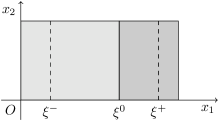
Let us consider rectangular domain in two-dimensional space $R^{2}$ with boundary $\Gamma$:

$$\{(x_{1},x_{2})\ |\ 0\leq x_{1}\leq 1,\ 0\leq x_{2}\leq 1\}.$$

Suppose, $0<\xi^{0}<1$, and define the segment $\{(x_{1},x_{2})\ |\ x_{1}=\xi^{0},\ 0\leq x_{2}\leq 1\}$ (see Figure 1).

We consider the following nonlocal contact problem: Find the continuous function

$$u(x_{1},x_{2})=\begin{cases}u^{-}(x_{1},x_{2}),&0\leq x_{1}<\xi^{0},\ 0\leq x_{2}\leq 1,\\ u(\xi^{0},x_{2}),&x_{1}=\xi^{0},\ 0\leq x_{2}\leq 1,\\ u^{+}(x_{1},x_{2}),&\xi^{0}<x_{1}\leq 1,\ 0\leq x_{2}\leq 1,\end{cases}$$ (1)

which satisfies the equations:

$\displaystyle\Delta u^{-}(x_{1},x_{2})$ $\displaystyle=f^{-}(x_{1},x_{2}),$ $\displaystyle 0<x_{1}<\xi^{0},\ 0<x_{2}<1,$ (2)
$\displaystyle\Delta u^{+}(x_{1},x_{2})$ $\displaystyle=f^{+}(x_{1},x_{2}),$ $\displaystyle\xi^{0}<x_{1}<1,\ 0<x_{2}<1,$

the boundary conditions

$$\begin{gathered}\left.\begin{aligned} u^{-}(x_{1},0)&=0,&&0\leq x_{1}\leq\xi^{0},\\ u^{+}(x_{1},0)&=0,&&\xi^{0}\leq x_{1}\leq 1,\end{aligned}\right\}\\ \left.\begin{aligned} u^{-}(x_{1},1)&=0,&&0\leq x_{1}\leq\xi^{0},\\ u^{+}(x_{1},1)&=0,&&\xi^{0}\leq x_{1}\leq 1,\end{aligned}\right\}\\ \left.\begin{aligned} u^{-}(0,x_{2})&=0,&&0\leq x_{2}\leq 1,\\ u^{+}(1,x_{2})&=0,&&0\leq x_{2}\leq 1,\end{aligned}\right\}\end{gathered}$$ (3)

and the nonlocal contact condition

$$u^{-}(\xi^{0},x_{2})=u^{+}(\xi^{0},x_{2})=u(\xi^{0},x_{2})=u_{0}(x_{2})\\ =\gamma^{-}u^{-}(\xi^{-},x_{2})+\gamma^{+}u^{+}(\xi^{+},x_{2})+\phi_{0}(\xi^{0},x_{2}),\qquad 0<x_{2}<1,$$ (4)

where $f^{-}(x_{1},x_{2}),\,f^{+}(x_{1},x_{2})$ are known, sufficiently smooth functions, and

$$0<\xi^{-}<\xi^{0},\,\xi^{0}<\xi^{+}<1,\,\gamma^{-}>0,\,\gamma^{+}>0,\,\gamma^{-}+\gamma^{+}\leq 1.$$ (5)
Refer to caption
Figure 1: Domain for Poisson equation

Note that in previously published articles the nonlocal conditions were mainly formulated under the restriction of the following type: $\gamma^{-}+\gamma^{+}<1$. In this article the results are achieved considering the following conditions $\gamma^{-}+\gamma^{+}\leq 1$.

2.2 Separation of variables

Using the method of separation of variables, we can build the solution of nonlocal contact problem (1)-(5). Note that this technique can be extended for more general case.

We will find the solution of nonlocal contact problem (1)-(5) in a following form:

$\displaystyle u^{-}(x_{1},x_{2})$ $\displaystyle=\sum_{k=1}^{\infty}a_{k}^{-}(x_{1})\sin k\pi x_{2},$ $\displaystyle 0\leq x_{1}\leq\xi^{0},\ 0\leq x_{2}\leq 1,$ (6)
$\displaystyle u^{+}(x_{1},x_{2})$ $\displaystyle=\sum_{k=1}^{\infty}a_{k}^{+}(x_{1})\sin k\pi x_{2},$ $\displaystyle\xi^{0}\leq x_{1}\leq 1,\ 0\leq x_{2}\leq 1.$ (7)

It is evident that the functions (6) and (7) satisfy the boundary conditions:

$\displaystyle u^{-}(x_{1},0)$ $\displaystyle=u^{-}(x_{1},1)=0,$ $\displaystyle 0\leq x_{1}\leq\xi^{0},$
$\displaystyle u^{+}(x_{1},0)$ $\displaystyle=u^{+}(x_{1},1)=0,$ $\displaystyle\xi^{0}\leq x_{1}\leq 1.$

We must choose the coefficients $a_{k}^{+}(x_{1})$ and $a_{k}^{-}(x_{1}),\ k=1,2,3,\ldots,$ so that the functions (6), (7) satisfy the equations (2), the rest boundary conditions

$$u^{-}(0,x_{2})=0,\ u^{+}(1,x_{2})=0,\qquad 0\leq x_{2}\leq 1,$$

and the nonlocal contact condition as well. Thus, $a_{k}^{+}(x_{1})$ and $a_{k}^{-}(x_{1}),\ k=1,2,3,…,$ should be solutions of the following problems:

$\displaystyle\frac{d^{2}a_{k}^{-}(x_{1})}{dx_{1}^{2}}-\lambda_{k}^{2}a_{k}^{-}(x_{1})$ $\displaystyle=f_{k}^{-}(x_{1}),$ $\displaystyle 0<x_{1}<\xi^{0},\ a_{k}^{-}(0)=0,\ a_{k}^{-}(\xi^{0})=\Phi_{k},$ (8)
$\displaystyle\frac{d^{2}a_{k}^{+}(x_{1})}{dx_{1}^{2}}-\lambda_{k}^{2}a_{k}^{+}(x_{1})$ $\displaystyle=f_{k}^{+}(x_{1}),$ $\displaystyle\xi^{0}<x_{1}<1,\ a_{k}^{+}(\xi^{0})=\Phi_{k},\ a_{k}^{+}(1)=0,$ (9)

where $\lambda_{k}=\pi^{2}k^{2},\ f_{k}^{-}(x_{1}),\ f_{k}^{+}(x_{1})$ are the coefficients of Fourier Series expansion of the functions $f^{-}(x_{1},x_{2})$ and $f^{+}(x_{1},x_{2})$:

$$f^{-}(x_{1},x_{2})=\sum_{k=1}^{\infty}f_{k}^{-}(x_{1})\sin\lambda_{k}x_{2},\qquad f^{+}(x_{1},x_{2})=\sum_{k=1}^{\infty}f_{k}^{+}(x_{1})\sin\lambda_{k}x_{2},$$

and $\Phi_{k}$, $k=1,2,\ldots,$ are so far unknown constants

$$u(\xi^{0},x_{2})=u_{0}(x_{2})=\sum_{k=1}^{\infty}\Phi_{k}\sin\lambda_{k}x_{2}.$$ (10)

2.3 Existence and uniqueness of the solution

Using the method of constructing general solutions of differential equations with homogeneous boundary conditions and method of variation of constants or method of undetermined coefficients of Lagrange (see, for example [20]), it is possible to build the general solutions of equations (8) and (9).

At first, we will consider the problem (8). The general solution of the problem (8) can be written in the following form:

$$a_{k}^{-}(x_{1})=\tilde{c}_{1}^{-}(x_{1})e^{\sqrt{\lambda_{k}}x_{1}}+\tilde{c}_{2}^{-}(x_{1})e^{-\sqrt{\lambda_{k}}x_{1}}\\ +\frac{1}{\sqrt{\lambda_{k}}}\int_{0}^{x_{1}}\sinh\left(\sqrt{\lambda_{k}}(x_{1}-s)\right)f_{k}^{-}(s)\,ds,\qquad k=1,2,\ldots,$$

where we can define $\tilde{c}_{1}^{-}(x_{1})$, $\tilde{c}_{2}^{-}(x_{1})$, considering the boundary conditions $a_{k}^{-}(0)=0$, $a_{k}^{-}(\xi^{0})=\Phi_{k}$.

Finally the general solution of the problem (8) will get the following form:

$$a_{k}^{-}(x_{1})=\frac{(\Phi_{k}-I^{-})\sinh(\sqrt{\lambda_{k}}x_{1})}{\sinh(\sqrt{\lambda_{k}}\xi^{0})}+\frac{1}{\sqrt{\lambda_{k}}}\int_{0}^{x_{1}}\sinh\left(\sqrt{\lambda_{k}}(x_{1}-s)\right)f_{k}^{-}(s)\,ds,\\ k=1,2,\ldots$$

where

$$I^{-}=\frac{1}{\sqrt{\lambda_{k}}}\int_{0}^{\xi^{0}}\sinh\left(\sqrt{\lambda_{k}}(\xi^{0}-s)\right)\,f_{k}^{-}(s)\,ds.$$ (11)

Consequently, the formal solution of the problem (2)-(3) on the left subarea is the following function

$$u^{-}(x_{1},x_{2})=\sum_{k=1}^{\infty}\left[\frac{(\Phi_{k}-I^{-})\sinh(\sqrt{\lambda_{k}}x_{1})}{\sinh(\sqrt{\lambda_{k}}\xi^{0})}\right.\\ \left.+\frac{1}{\sqrt{\lambda_{k}}}\int_{0}^{x_{1}}\sinh\left(\sqrt{\lambda_{k}}(x_{1}-s)\right)f_{k}^{-}(s)\,ds\right]\sin\lambda_{k}x_{2},$$

where $I^{-}$ is defined using (11).

Analogously, the general solution of the problem (9) can be written in the following form:

$$a_{k}^{+}(x_{1})=\tilde{c}_{1}^{+}(x_{1})e^{\sqrt{\lambda_{k}}x_{1}}+\tilde{c}_{2}^{+}(x_{1})e^{-\sqrt{\lambda_{k}}x_{1}}\\ +\frac{1}{\sqrt{\lambda_{k}}}\int_{\xi^{0}}^{x_{1}}\sinh\left(\sqrt{\lambda_{k}}(x_{1}-s)\right)f_{k}^{+}(s)\,ds,\qquad k=1,2,\ldots$$

Considering the boundary conditions $a_{k}^{+}(\xi^{0})=\Phi_{k}$, $a_{k}^{+}(1)=0$, we can define $\tilde{c}_{1}^{+}$, $\tilde{c}_{2}^{+}$ uniquely.

Finally we can describe the formal solution of the problem (2)-(3) on the right subarea in a following way:

$$u^{+}(x_{1},x_{2})=\sum_{k=1}^{\infty}\left[\frac{(\Phi_{k}\sinh(\sqrt{\lambda_{k}}(x_{1}-1))-I^{+}\sinh(\sqrt{\lambda_{k}}(x_{1}-\xi^{0}))}{\sinh(\sqrt{\lambda_{k}}(\xi^{0}-1))}\right.\\ \left.+\frac{1}{\sqrt{\lambda_{k}}}\int_{\xi^{0}}^{x_{1}}\sinh(\sqrt{\lambda_{k}}(x_{1}-s))f_{k}^{+}(s)ds\right]\sin\lambda_{k}x_{2},$$

where

$$I^{+}=\frac{1}{\sqrt{\lambda_{k}}}\int_{\xi^{0}}^{1}\sinh(\sqrt{\lambda_{k}}(1-s))f_{k}^{+}(s)ds.$$ (12)

We can define the coefficients $\Phi_{k}$, $k=1,2,\ldots$, using the equality (10) and nonlocal contact condition (4):

$$\Phi_{k}=\gamma^{-}\frac{\Phi_{k}\sinh(\sqrt{\lambda_{k}}\xi^{-})}{\sinh(\sqrt{\lambda_{k}}\xi^{0})}+\gamma^{+}\frac{\Phi_{k}\sinh(\sqrt{\lambda_{k}}(\xi^{+}-1))}{\sinh(\sqrt{\lambda_{k}}(\xi^{0}-1))}\\ -(F_{k}^{-}+F_{k}^{+})+\frac{\gamma^{-}}{\sqrt{\lambda_{k}}}\int_{0}^{\xi^{-}}\sinh(\sqrt{\lambda_{k}}(\xi^{-}-s))f_{k}^{-}(s)ds\\ +\frac{\gamma^{+}}{\sqrt{\lambda_{k}}}\int_{\xi^{0}}^{\xi^{+}}\sinh(\sqrt{\lambda_{k}}(\xi^{+}-s))f_{k}^{+}(s)ds+\phi_{0k},$$

where

$\displaystyle\phi_{0}(\xi^{0},x_{2})$ $\displaystyle=\sum_{k=1}^{\infty}\phi_{0k}\sin\lambda_{k}x_{2},$
$\displaystyle F_{k}^{-}$ $\displaystyle=\gamma^{-}\frac{\sinh(\sqrt{\lambda_{k}}\xi^{-})}{\sqrt{\lambda_{k}}\sinh(\sqrt{\lambda_{k}}\xi^{0})}\int_{0}^{\xi^{0}}\sinh(\sqrt{\lambda_{k}}(\xi^{0}-s))f_{k}^{-}(s)ds,$
$\displaystyle F_{k}^{+}$ $\displaystyle=\gamma^{+}\frac{\sinh(\sqrt{\lambda_{k}}(\xi^{+}-\xi^{0}))}{\sqrt{\lambda_{k}}\sinh(\sqrt{\lambda_{k}}(\xi^{0}-1))}\int_{\xi^{0}}^{1}\sinh(\sqrt{\lambda_{k}}(1-s))f_{k}^{+}(s)ds.$

Then we will get

$$\Phi_{k}\left\{1-\left[\gamma^{-}\frac{\sinh(\sqrt{\lambda_{k}}\xi^{-})}{\sinh(\sqrt{\lambda_{k}}\xi^{0})}+\gamma^{+}\frac{\sinh(\sqrt{\lambda_{k}}(\xi^{+}-1))}{\sinh(\sqrt{\lambda_{k}}(\xi^{0}-1))}\right]\right\}=-F_{k}+\phi_{0k},$$ (13)

where

$$F_{k}=F_{k}^{-}+F_{k}^{+}-\left[\frac{\gamma^{-}}{\sqrt{\lambda_{k}}}\int_{0}^{\xi^{-}}\sinh(\sqrt{\lambda_{k}}(\xi^{-}-s))f_{k}^{-}(s)ds\right.\\ \left.+\frac{\gamma^{+}}{\sqrt{\lambda_{k}}}\int_{\xi^{0}}^{\xi^{+}}\sinh(\sqrt{\lambda_{k}}(\xi^{+}-s))f_{k}^{+}(s)ds\right].$$ (14)

As

$$\frac{\sinh(\sqrt{\lambda_{k}}\xi^{-})}{\sinh(\sqrt{\lambda_{k}}\xi^{0})}<1\ \mbox{ and }\ \frac{\sinh(\sqrt{\lambda_{k}}(\xi^{+}-1))}{\sinh(\sqrt{\lambda_{k}}(\xi^{0}-1))}<1,$$

then we will have

$$1-\left[\gamma^{-}\frac{\sinh(\sqrt{\lambda_{k}}\xi^{-})}{\sinh(\sqrt{\lambda_{k}}\xi^{0})}+\gamma^{+}\frac{\sinh(\sqrt{\lambda_{k}}(\xi^{+}-1))}{\sinh(\sqrt{\lambda_{k}}(\xi^{0}-1))}\right]>1-(\gamma^{-}+\gamma^{+})\geq 0.$$

Consequently, from the equality (13) we get

$$\Phi_{k}=\left\{1-\left[\gamma^{-}\frac{\sinh(\sqrt{\lambda_{k}}\xi^{-})}{\sinh(\sqrt{\lambda_{k}}\xi^{0})}+\gamma^{+}\frac{\sinh(\sqrt{\lambda_{k}}(\xi^{+}-1))}{\sinh(\sqrt{\lambda_{k}}(\xi^{0}-1))}\right]\right\}^{-1}(-F_{k}+\phi_{0k}),\\ k=1,2,\ldots,$$ (15)

where $F_{k}$ is defined from (14). Finally, the formal solution of the problem (2)-(4) is the following function:

$$u(x_{1},x_{2})=\begin{cases}u^{-}(x_{1},x_{2}),&0\leq x_{1}<\xi^{0},\ 0\leq x_{2}\leq 1,\\ u(\xi^{0},x_{2}),&x_{1}=\xi^{0},\ 0\leq x_{2}\leq 1,\\ u^{+}(x_{1},x_{2}),&\xi^{0}<x_{1}\leq 1,\ 0\leq x_{2}\leq 1,\end{cases}$$

where

$$u^{-}(x_{1},x_{2})=\sum_{k=1}^{\infty}\left[\frac{(\Phi_{k}-I^{-})\sinh(\sqrt{\lambda_{k}}x_{1})}{\sinh(\sqrt{\lambda_{k}}\xi^{0})}\right.\\ \left.+\frac{1}{\sqrt{\lambda_{k}}}\int_{0}^{x_{1}}\sinh(\sqrt{\lambda_{k}}(x_{1}-s))f_{k}^{-}(s)ds\right]\sin\lambda_{k}x_{2},$$
$$u(\xi^{0},x_{2})=\sum_{k=1}^{\infty}\Phi_{k}\sin\lambda_{k}x_{2},$$
$$u^{+}(x_{1},x_{2})=\sum_{k=1}^{\infty}\left[\frac{(\Phi_{k}\sinh(\sqrt{\lambda_{k}}(x_{1}-1))-I^{+}\sinh(\sqrt{\lambda_{k}}(x_{1}-\xi^{0}))}{\sinh(\sqrt{\lambda_{k}}(\xi^{0}-1))}\right.\\ \left.+\frac{1}{\sqrt{\lambda_{k}}}\int_{\xi^{0}}^{x_{1}}\sinh(\sqrt{\lambda_{k}}(x_{1}-s))f_{k}^{+}(s)ds\right]\sin\lambda_{k}x_{2},$$

$\Phi_{k}$ is defined from (15), and $I^{-},\ I^{+}$ - from (11) and (12), respectively.

Thus, the following theorem is true.

Theorem 1.

If $f^{-}(x_{1},x_{2}),\ f^{+}(x_{1},x_{2})$ and $\phi_{0}(\xi^{0},x_{2})$ are sufficiently smooth functions, then the problem (2)-(4) has a unique regular solution.

Note, that the applied technique can be successfully used for more general problems, but in this case the use of spectral theory of linear operators will be needed.

3 Nonlocal Contact Problem for Equation with Variable Coefficients

3.1 Designations

Refer to caption
Figure 2: Domain for contact problem for equation with variable coefficients, $\bar{D}=D\cup\gamma$

Now let us consider the problem with nonlocal contact conditions for elliptic equation with variable coefficients.
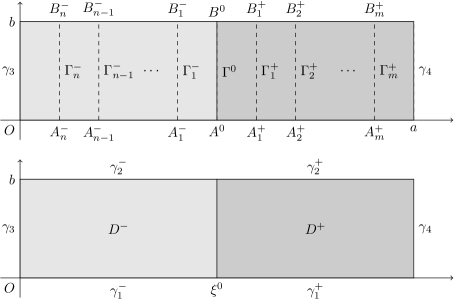
Suppose $D$ is a rectangular domain in two-dimensional space $R^{2}$ (see Figure 2): $D=\{(x_{1},x_{2})\ |\ 0<x_{1}<a,\ 0<x_{2}<b\}$ with piecewise boundary $\gamma=\bigcup_{i=1}^{4}\gamma_{i}$, where

$\displaystyle\gamma_{1}$ $\displaystyle=\{(x_{1},x_{2})\ |\ 0\leq x_{1}\leq a,\ x_{2}=0\},$ $\displaystyle\gamma_{2}$ $\displaystyle=\{(x_{1},x_{2})\ |\ 0\leq x_{1}\leq a,\ x_{2}=b\},$
$\displaystyle\gamma_{3}$ $\displaystyle=\{(x_{1},x_{2})\ |\ x_{1}=0,\ 0\leq x_{2}\leq b\},$ $\displaystyle\gamma_{4}$ $\displaystyle=\{(x_{1},x_{2})\ |\ x_{1}=a,\ 0\leq x_{2}\leq b\}.$

Suppose, $0<\xi^{0}<a$, and define:

$\displaystyle\Gamma^{0}$ $\displaystyle=\{(x_{1},x_{2})\ |\ x_{1}=\xi^{0},0\leq x_{2}\leq b\}$
$\displaystyle\gamma_{1}^{-}$ $\displaystyle=\{(x_{1},x_{2})\ |\ 0\leq x_{1}\leq\xi^{0},x_{2}=0\},$ $\displaystyle\gamma_{2}^{-}$ $\displaystyle=\{(x_{1},x_{2})\ |\ 0\leq x_{1}\leq\xi^{0},x_{2}=b\},$
$\displaystyle\gamma_{1}^{+}$ $\displaystyle=\{(x_{1},x_{2})\ |\ \xi^{0}\leq x_{1}\leq a,x_{2}=0\},$ $\displaystyle\gamma_{2}^{+}$ $\displaystyle=\{(x_{1},x_{2})\ |\ \xi^{0}\leq x_{1}\leq a,x_{2}=b\}.$

It is obvious, that $\gamma_{1}^{-}\cup\gamma_{1}^{+}=\gamma_{1}$, $\gamma_{2}^{-}\cup\gamma_{2}^{+}=\gamma_{2}$, and $\Gamma^{0}$ divides the domain $D$ into two parts (subdomains) $D^{-}$ and $D^{+}$ , where

$$D^{-}=\{(x_{1},x_{2})\ |\ 0<x_{1}<\xi^{0},0<x_{2}<b\},\qquad D^{+}=\{(x_{1},x_{2})\ |\ \xi^{0}<x_{1}<a,0<x_{2}<b\}$$
$$\Gamma_{i}^{-}=\{(x_{1},x_{2})\ |\ x_{1}=\xi_{i}^{-},\ 0<\xi_{i}^{-}<\xi^{0},\ 0\leq x_{2}\leq b\},\\ i=\textasciimacron\overline{(1,n)},\ 0<\xi_{n}^{-}<\cdots<\xi_{1}^{-}<\xi^{0},$$
$$\Gamma_{j}^{+}=\{(x_{1},x_{2})\ |\ x_{1}=\xi_{j}^{+},\ \xi^{0}<\xi_{j}^{+}<a,\ 0\leq x_{2}\leq b\},\\ j=\overline{(1,m)},\ \xi^{0}<\xi_{1}^{+}<\xi_{2}^{+}<\cdots<\xi_{m}^{+}<b.$$

$\Gamma^{0},\Gamma_{i}^{-},\ i=\overline{(1,n)},$ and $\Gamma_{j}^{+},\ j=\overline{(1,m)},$ intersect $\gamma_{1}$ and $\gamma_{2}$, respectively, in the points:

$$A^{0}(\xi^{0},0),\ B^{0}(\xi^{0},b),\ A_{i}^{-}(\xi_{i}^{-},0),\ B_{i}^{-}(\xi_{i}^{-},b),\ A_{i}^{+}(\xi_{i}^{+},0)\text{ and }B_{i}^{+}(\xi_{i}^{+},b).$$

3.2 Statement of the Problem

Let us consider the following problem: Find in domain $\bar{D}=D\cup\gamma$ (where $\gamma$ is defined in 3.1) a continuous function $u(x_{1},x_{2})$:

$$\begin{gathered}u(x_{1},x_{2})=\begin{cases}u^{-}(x_{1},x_{2}),&\mbox{ if }(x_{1},x_{2})\in D^{-},\\ u^{0}(x_{1},x_{2}),&\mbox{ if }(x_{1},x_{2})\in\Gamma^{0},\\ u^{+}(x_{1},x_{2}),&\mbox{ if }(x_{1},x_{2})\in D^{+},\end{cases}\\ u^{-}(x_{1},x_{2})\in C^{2}(D^{-}),\ u^{+}(x_{1},x_{2})\in C^{2}(D^{+}),\ u^{0}(x_{1},x_{2})\in C(\Gamma^{0}),\end{gathered}$$ (16)

which satisfies the equations

$$L^{-}u^{-}(x_{1},x_{2})\equiv\\ \sum_{\alpha,\beta=1}^{2}\frac{\partial}{\partial x_{\alpha}}(K_{\alpha\beta}^{-}(x_{1},x_{2})\frac{\partial u^{-}}{\partial x_{\beta}})-k^{-}(x_{1},x_{2})u^{-}=-f^{-}(x_{1},x_{2}),\ (x_{1},x_{2})\in D^{-},$$ (17)
$$L^{+}u^{+}(x_{1},x_{2})\equiv\\ \sum_{\alpha,\beta=1}^{2}\frac{\partial}{\partial x_{\alpha}}(K_{\alpha\beta}^{+}(x_{1},x_{2})\frac{\partial u^{+}}{\partial x_{\beta}})-k^{+}(x_{1},x_{2})u^{+}=-f^{+}(x_{1},x_{2}),\ (x_{1},x_{2})\in D^{+},$$ (18)

The function $u(x_{1},x_{2})$ also satisfies the boundary conditions

$\displaystyle u^{-}(x_{1},x_{2})$ $\displaystyle=\phi^{-}(x_{1},x_{2}),$ $\displaystyle(x_{1},x_{2})\in\gamma_{1}^{-}\cup\gamma_{2}^{-}\cup\gamma_{3},$
$\displaystyle u^{+}(x_{1},x_{2})$ $\displaystyle=\phi^{+}(x_{1},x_{2}),$ $\displaystyle(x_{1},x_{2})\in\gamma_{1}^{+}\cup\gamma_{2}^{+}\cup\gamma_{4},$

the nonlocal contact conditions

$$u^{-}(\Gamma^{0})=u^{+}(\Gamma^{0})=u(\Gamma^{0})=\sum_{i=1}^{n}\beta_{i}^{-}u^{-}(\Gamma_{i}^{-})+\sum_{j=1}^{m}\beta_{j}^{+}u^{+}(\Gamma_{j}^{+})+\phi^{0}(\Gamma^{0}),$$

and the coordination conditions

$\displaystyle u(A^{0})$ $\displaystyle=\sum_{i=1}^{n}\beta_{i}^{-}u^{-}(A_{i}^{-})+\sum_{j=1}^{m}\beta_{j}^{+}u^{+}(A_{j}^{+})+\phi^{0}(A^{0}),$ (19)
$\displaystyle u(B^{0})$ $\displaystyle=\sum_{i=1}^{n}\beta_{i}^{-}u^{-}(B_{i}^{-})+\sum_{j=1}^{m}\beta_{j}^{+}u^{+}(B_{j}^{+})+\phi^{0}(B^{0}),$

where $\beta_{i}^{-}=\text{const}>0$, $\beta_{j}^{+}=\text{const}>0$, $0<\sum_{i=1}^{n}\beta_{i}^{-}+\sum_{j=1}^{m}\beta_{j}^{+}\leq 1.$ $K_{\alpha\beta}^{\pm}(\cdot),$ $k^{\mp}(\cdot)\ f^{\pm}(\cdot)$, $\phi^{\pm}(\cdot)$ and $\phi^{0}(\cdot)$ are known functions, which satisfy all the conditions, that provide existence of the unique solutions of Dirichlet problem in $D^{-}$ and $D^{+}$ [21].

Suppose that the equations (17) and (18) are uniformly elliptic. Then their coefficients satisfy the following conditions [21]:

$\displaystyle 4K_{11}^{-}(x_{1},x_{2})\cdot K_{22}^{-}(x_{1},x_{2})$ $\displaystyle>(K_{12}^{-}(x_{1},x_{2})+K_{21}^{-}(x_{1},x_{2}))^{2},$
$\displaystyle 4K_{11}^{+}(x_{1},x_{2})\cdot K_{22}^{+}(x_{1},x_{2})$ $\displaystyle>(K_{12}^{+}(x_{1},x_{2})+K_{21}^{+}(x_{1},x_{2}))^{2}.$

$K^{-}_{\alpha\beta}(x_{1},x_{2})$ and $u^{-}(x_{1},x_{2})$ can be considered as coefficient of heat conductivity and temperature of the first body ($D^{-}$), $K^{+}_{\alpha\beta}(x_{1},x_{2})$ and $u^{+}(x_{1},x_{2})$ - of the second body ($D^{+}$). Thus, the stated problem can be considered as a mathematical model of stationary distribution of heat in two contacting isotropic bodies.

We will call the problem (16)-(19) nonlocal contact one since it is generalization of a classical contact problem.

3.3 Uniqueness of a Solution of Problem (16)-(19)

The following theorem is true.

Theorem 2.

If the regular solution of problem (16)-(19) exists and condition $0<\sum_{i=1}^{n}\beta_{i}^{-}+\sum_{j=1}^{m}\beta_{j}^{+}\leq 1$ is fulfilled, then then the solution is unique.

Proof.

Suppose that problem (16)-(19) has two solutions: $v(x_{1},x_{2})$ and $w(x_{1},x_{2})$. Then for the function $z(x_{1},x_{2})=v(x_{1},x_{2})-w(x_{1},x_{2})$ we will have the following problem

$\displaystyle L^{-}z^{-}(x_{1},x_{2})$ $\displaystyle=0,\text{ if }(x_{1},x_{2})\in D^{-},$
$\displaystyle L^{+}z^{+}(x_{1},x_{2})$ $\displaystyle=0,\text{ if }(x_{1},x_{2})\in D^{+},$
$\displaystyle z^{-}(x_{1},x_{2})$ $\displaystyle=0,$ $\displaystyle\text{ if }(x_{1},x_{2})\in\gamma_{1}^{-}\cup\gamma_{2}^{-}\cup\gamma_{3},$ (20)
$\displaystyle z^{+}(x_{1},x_{2})$ $\displaystyle=0,$ $\displaystyle\text{ if }(x_{1},x_{2})\in\gamma_{1}^{+}\cup\gamma_{2}^{+}\cup\gamma_{4},$
$$z(\Gamma^{0})=z^{-}(\Gamma^{0})=z^{+}(\Gamma^{0})=\sum_{i=1}^{n}\beta_{i}^{-}z^{-}(\Gamma_{i}^{-})+\sum_{j=1}^{m}\beta_{j}^{+}z^{+}(\Gamma_{j}^{+}).$$ (21)

From the equality (21) it follows that

$$\max|z(\Gamma^{0})|\leq\max\sum_{i=1}^{n}\beta_{i}^{-}|z^{-}(\Gamma_{i}^{-})|+\max\sum_{j=1}^{m}\beta_{j}^{+}|z^{+}(\Gamma_{j}^{+})|\\ \leq\max_{0\leq i\leq n}|z^{-}(\Gamma_{i}^{-})|\sum_{i=1}^{n}\beta_{i}^{-}+\max_{0\leq j\leq m}|z^{+}(\Gamma_{j}^{+})|\sum_{j=1}^{m}\beta_{j}^{+}.$$

Taking into account the condition $0<\sum_{i=1}^{n}\beta_{i}^{-}+\sum_{j=1}^{m}\beta_{j}^{+}\leq 1$, we obtain

$$\max|z(\Gamma_{0})|\leq\max_{0\leq i\leq n}|z^{-}(\Gamma_{i}^{-})|\ \mbox{ or }\ \max|z(\Gamma_{0})|\leq\max_{0\leq j\leq m}|z^{+}(\Gamma_{j}^{+})|.$$

This means that the function z does not attain a maximum on $\Gamma_{0}$, but attains its maximum on $D^{-}$ or $D^{+}$, that contradicts the maximum principle. So, $z\equiv\text{const}$ and taking into account condition (20), we obtain $z\equiv 0$, i.e. the solution of the problem (16) - (19) is unique. ∎

3.4 Iterative Method for Problem (16)-(19)

Let us consider the following iteration process for the problem (16)-(19):

$\displaystyle L^{-}[u^{-}(x_{1},x_{2})]^{(k)}$ $\displaystyle=-f^{-}(x_{1},x_{2}),$ $\displaystyle\mbox{if }(x_{1},x_{2})\in D^{-},$ (22)
$\displaystyle L^{+}[u^{+}(x_{1},x_{2})]^{(k)}$ $\displaystyle=-f^{+}(x_{1},x_{2}),$ $\displaystyle\mbox{if }(x_{1},x_{2})\in D^{+},$ (23)
$\displaystyle[u^{-}(x_{1},x_{2})]^{(k)}$ $\displaystyle=\phi^{-}(x_{1},x_{2}),$ $\displaystyle\mbox{if }(x_{1},x_{2})\in\gamma_{1}^{-}\cup\gamma_{2}^{-}\cup\gamma_{3},$ (24)
$\displaystyle[u^{+}(x_{1},x_{2})]^{(k)}$ $\displaystyle=\phi^{+}(x_{1},x_{2}),$ $\displaystyle\mbox{if }(x_{1},x_{2})\in\gamma_{1}^{+}\cup\gamma_{2}^{+}\cup\gamma_{4},$ (25)
$$u^{(k)}(\Gamma^{0})=[u^{-}(\Gamma^{0})]^{(k)}=[u^{+}(\Gamma^{0})]^{(k)}\\ =\sum_{i=1}^{n}\beta_{i}^{-}[u^{-}(\Gamma_{i}^{-})]^{(k-1)}+\sum_{j=1}^{m}\beta_{j}^{+}[u^{+}(\Gamma_{j}^{+})]^{(k-1)}+\phi^{0}(\Gamma^{0}),$$ (26)

where $k=1,2,\ldots$. Initially we can take e.g. $[u^{-}(\Gamma_{i}^{-})]^{(0)}=0,$ $[u^{+}(\Gamma_{j}^{+})]^{(0)}=0,$ $i=\overline{(1,n)},\ j=\overline{(1,m)}.$

Given the initial approximations in nonlocal contact condition (26) of the iterative process (20)-(26), $\left[u^{-}(\Gamma^{-}_{i})\right]^{(k-1)}$ and $\left[u^{+}(\Gamma^{+}_{j})\right]^{(k-1)}$, $i=\overline{(1,n)}$, $j=\overline{(1,m)}$, we can calculate the values of $u$ on $\Gamma^{0}$ and, thus, get two classical boundary problems. After solving these problems, we can define the consequent values of $u$ on $\Gamma^{0}$ from (26) for the next iteration, etc.

Theorem 3.

If the solution of problem (16)-(19) exists, then the iterative process (22)-(26) converges to this solution at the rate of an infinitely decreasing geometric progression.

Proof.

Denote by $z^{(k)}(x_{1},x_{2})=u^{(k)}(x_{1},x_{2})-u(x_{1},x_{2})$, where $u$ is a solution of the problem (16)-(19) and $u^{(k)}$ – of the problem (22)-(26).

Then we obtain the following problems:

$\displaystyle L^{-}[z^{-}(x_{1},x_{2})]^{(k)}$ $\displaystyle=0,$ $\displaystyle\text{if }(x_{1},x_{2})\in D^{-},$
$\displaystyle L^{+}[z^{+}(x_{1},x_{2})]^{(k)}$ $\displaystyle=0,$ $\displaystyle\text{if }(x_{1},x_{2})\in D^{+},$
$\displaystyle[z^{-}(x_{1},x_{2})]^{(k)}$ $\displaystyle=0,$ $\displaystyle\text{if }(x_{1},x_{2})\in\gamma_{1}^{-}\cup\gamma_{2}^{-}\cup\gamma_{3},$
$\displaystyle[z^{+}(x_{1},x_{2})]^{(k)}$ $\displaystyle=0,$ $\displaystyle\text{if }(x_{1},x_{2})\in\gamma_{1}^{+}\cup\gamma_{2}^{+}\cup\gamma_{4},$
$$[z(\Gamma^{0})]^{(k)}=[z^{-}(\Gamma^{0})]^{(k)}=[z^{+}(\Gamma^{0})]^{(k)}\\ =\sum_{i=1}^{n}\beta_{i}^{-}[z^{-}(\Gamma_{i}^{-})]^{(k-1)}+\sum_{j=1}^{m}\beta_{j}^{+}[z^{+}(\Gamma_{j}^{+})]^{(k-1)},$$ (27)

where $k=1,2,\ldots,$ and $[z^{-}(\Gamma_{i}^{-})]^{(0)}=0,$ $[z^{+}(\Gamma_{j}^{+})]^{(0)}=0,$ $i=\overline{(1,n)},\ j=\overline{(1,m)}.$
From the equality (27) we have

$$\max_{\Gamma^{0}}\left|[z(\Gamma^{0})]^{(k)}\right|\leq\max_{1\leq i\leq n}\left|[z^{-}(\Gamma_{i}^{-})]^{(k-1)}\right|\sum_{i=1}^{n}\beta_{i}^{-}+\max_{1\leq j\leq m}\left|[z^{+}(\Gamma_{j}^{+})]^{(k-1)}\right|\sum_{j=1}^{m}\beta_{j}^{+}.$$

If we use Schwarz’ lemma [19], we will get inequalities:

$\displaystyle\max_{1\leq i\leq n}|[z^{-}(\Gamma_{i}^{-})]^{(k-1)}|$ $\displaystyle\leq q^{-}\max_{\Gamma^{0}}|[z(\Gamma^{0})]^{(k-1)}|,$ (28)
$\displaystyle\max_{1\leq j\leq m}|[z^{+}(\Gamma_{j}^{+})]^{(k-1)}|$ $\displaystyle\leq q^{+}\max_{\Gamma^{0}}|[z(\Gamma^{0})]^{(k-1)}|,$ (29)

where $q^{+}=const,\ 0<q^{+}<1,\ q^{-}=const,\ 0<q^{-}<1$. Note, that these constants depend only on geometric properties of domains $D^{-}$ and $D^{+}$.

If we use inequalities (28), (29), then we have

$$\max_{\Gamma^{0}}|[z(\Gamma^{0})]^{(k)}|\leq q^{+}\sum_{j=1}^{m}\beta_{j}^{+}\cdot\max_{\Gamma^{0}}|[z(\Gamma^{0})]^{(k-1)}|+q^{-}\sum_{i=1}^{n}\beta_{i}^{-}\cdot\max_{\Gamma^{0}}|[z(\Gamma^{0})]^{(k-1)}|,$$

or

$$\max_{\Gamma^{0}}|[z(\Gamma^{0})]^{(k)}|\leq Q\max_{\Gamma^{0}}|[z(\Gamma^{0})]^{(k-1)}|,$$ (30)

where $Q=q^{+}\sum_{j=1}^{m}\beta_{j}^{+}+q^{-}\sum_{i=1}^{n}\beta_{i}^{-}.$

Taking into account the conditions $\beta_{i}^{-}=const>0$, $\beta_{j}^{+}=const>0$, $0<\sum_{j=1}^{m}\beta_{j}^{+}+\sum_{i=1}^{n}\beta_{i}^{-}\leq 1$, we obtain $0<Q<1$. This implies that

$$\lim_{k\to\infty}[z(\Gamma^{0})]^{(k)}=0.$$

If the solution of the problem (16)-(19) exists, then by the maximum principle we obtain

$\displaystyle\max_{D^{-}}\left|[u^{-}(x_{1},x_{2})]^{(k)}-u^{-}(x_{1},x_{2})\right|$ $\displaystyle=O(Q^{k}),$
$\displaystyle\max_{D^{+}}\left|[u^{+}(x_{1},x_{2})]^{(k)}-u^{+}(x_{1},x_{2})\right|$ $\displaystyle=O(Q^{k}),$

and, accordingly,

$$\max_{D}\left|[u(x_{1},x_{2})]^{(k)}-u(x_{1},x_{2})\right|=O(Q^{k}).$$

Thus, the iterative process (22)-(26) converges to this solution of the problem (16)-(19) at the rate of an infinitely decreasing geometric progression with ratio $Q$.

Remark.

By using the described iterative algorithm (22)-(26) the solution of a non–classical contact problem (16)-(19) is reduced to the solution of a sequence of classical boundary problems, which can be solved by any well-studied method.

3.5 Existence of a Solution of Problem (16)-(19)

Let us now prove the existence of a regular solution of the problem (16)-(19) in case of $f^{-}(x_{1},x_{2})\equiv 0$ and $f^{+}(x_{1},x_{2})\equiv 0$. We introduce the notation $\varepsilon^{(k)}(x_{1},x_{2})=u^{(k)}(x_{1},x_{2})-u^{(k-1)}(x_{1},x_{2})$. Then for the function $\varepsilon^{(k)}$ we obtain the following problem

$\displaystyle L^{-}[\varepsilon^{-}(x_{1},x_{2})]^{(k)}=$ $\displaystyle 0,$ $\displaystyle\text{ if }(x_{1},x_{2})\in D^{-},$
$\displaystyle L^{+}[\varepsilon^{+}(x_{1},x_{2})]^{(k)}=$ $\displaystyle 0,$ $\displaystyle\text{ if }(x_{1},x_{2})\in D^{+},$
$\displaystyle[\varepsilon^{-}(x_{1},x_{2})]^{(k)}=$ $\displaystyle 0,$ $\displaystyle\text{ if }(x_{1},x_{2})\in\gamma_{1}^{-}\cup\gamma_{2}^{-}\cup\gamma_{3},$
$\displaystyle[\varepsilon^{+}(x_{1},x_{2})]^{(k)}=$ $\displaystyle 0,$ $\displaystyle\text{ if }(x_{1},x_{2})\in\gamma_{1}^{+}\cup\gamma_{2}^{+}\cup\gamma_{4},$
$$[\varepsilon(\Gamma^{0})]^{(k)}=[\varepsilon^{-}(\Gamma^{0})]^{(k)}=[\varepsilon^{+}(\Gamma^{0})]^{(k)}=\sum_{i=1}^{n}\beta_{i}^{-}[\varepsilon^{-}(\Gamma_{i}^{-})]^{(k-1)}+\sum_{j=1}^{m}\beta_{j}^{+}[\varepsilon^{+}(\Gamma_{j}^{+})]^{(k-1)},$$

where $k=1,2,\ldots,$ and $[\varepsilon^{-}(\Gamma_{i}^{-})]^{(0)}=0,$ $[\varepsilon^{+}(\Gamma_{j}^{+})]^{(0)}=0,$ $i=\overline{(1,n)},\ j=\overline{(1,m)}.$

Then, analogously to (30), we obtain the estimation

$$\max_{\Gamma^{0}}|[\varepsilon(\Gamma^{0})]^{(k)}|\leq Q\max_{\Gamma^{0}}|[\varepsilon(\Gamma^{0})]^{(k-1)}|,\qquad 0<Q<1,$$

or

$$\max_{\Gamma^{0}}|u^{(k)}(\Gamma^{0})-u^{(k-1)}(\Gamma^{0})|\leq Q\max_{\Gamma^{0}}|u^{(k-1)}(\Gamma^{0})-u^{(k-2)}(\Gamma^{0})|,\qquad 0<Q<1,$$

This means that the sequence $\{u^{(k)}(x_{1},x_{2})\}$ converges uniformly on $\Gamma^{0}$. Then the functions $[u^{+}(x_{1},x_{2})]^{(k)}$ and $[u^{-}(x_{1},x_{2})]^{(k)}$ converge to the functions $u^{+}(x_{1},x_{2})$ and $u^{-}(x_{1},x_{2})$, respectively, on the domains $D^{-}$ and $D^{+}$ on the base of Harnack’s first theorem [26, 12].

From this we conclude that the limit function is the regular solution of the problem (16)-(19):

$$\lim_{k\rightarrow\infty}u^{(k)}(x_{1},x_{2})=u(x_{1},x_{2}).$$

4 Numerical Example

Let us consider the area $D=\{(x_{1},x_{2})|0<x_{1}<1,\ 0<x_{2}<1\}$ (see the Figure 3).

Refer to caption
Figure 3: Domain for numerical example

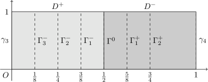
We consider the following test problem for the numerical solution: find in $\bar{D}$ a continuous function (16) $u(x_{1},x_{2})$, which satisfies the following equations:

$\displaystyle\frac{\partial}{\partial x_{1}}[(1+x_{1}^{2})\frac{\partial u^{-}}{\partial x_{1}}]+\frac{\partial}{\partial x_{2}}[(1+x_{2}^{2})\frac{\partial u^{-}}{\partial x_{2}}]$ $\displaystyle=f^{-}(x_{1},x_{2}),$ $\displaystyle\text{if }(x_{1},x_{2})\in D^{-},$
$\displaystyle\frac{\partial}{\partial x_{1}}[(1+2x_{1}^{2})\frac{\partial u^{+}}{\partial x_{1}}]+\frac{\partial}{\partial x_{2}}[(1+2x_{2}^{2})\frac{\partial u^{+}}{\partial x_{2}}]$ $\displaystyle=f^{+}(x_{1},x_{2}),$ $\displaystyle\text{if }(x_{1},x_{2})\in D^{+},$

where

$\displaystyle f^{-}(x_{1},x_{2})=$ $\displaystyle-\frac{1}{4}x_{1}x_{2}(-16+\pi^{2}(1+x_{2}^{2}))\cos\frac{\pi x_{2}}{2}-\pi x_{1}(1+2x_{2}^{2})\sin\frac{\pi x_{2}}{2}$
$\displaystyle f^{+}(x_{1},x_{2})=$ $\displaystyle-4x_{1}x_{2}\cos\frac{\pi x_{2}}{2}$
$\displaystyle+\frac{1}{4}(x_{1}-1)\left[x_{2}(-16+\pi^{2}(1+2x_{2}^{2}))\cos\frac{\pi x_{2}}{2}+4\pi(1+4x_{2}^{2})\sin\frac{\pi x_{2}}{2}\right],$

The function $u(x_{1},x_{2})$ also satisfies the boundary conditions

$\displaystyle u^{-}(x_{1},x_{2})$ $\displaystyle=0,$ $\displaystyle\text{if }(x_{1},x_{2})\in\gamma_{1}^{-}\cup\gamma_{2}^{-}\cup\gamma_{3},$
$\displaystyle u^{+}(x_{1},x_{2})$ $\displaystyle=0,$ $\displaystyle\text{if }(x_{1},x_{2})\in\gamma_{1}^{+}\cup\gamma_{2}^{+}\cup\gamma_{4},$

the nonlocal contact conditions

$$u^{-}(\frac{1}{2},x_{2})=u^{+}(\frac{1}{2},x_{2})=u(\Gamma^{0})=\frac{1}{8}u^{+}\left(\frac{5}{8},x_{2}\right)+\frac{1}{8}u^{+}\left(\frac{3}{4},x_{2}\right)\\ +\frac{1}{8}u^{-}\left(\frac{1}{8},x_{2}\right)+\frac{1}{8}u^{-}\left(\frac{1}{4},x_{2}\right)+\frac{1}{8}u^{-}\left(\frac{3}{8},x_{2}\right)+\frac{21}{64}x_{2}\cos\frac{\pi x_{2}}{2},$$

and the coordination conditions are fulfilled.

The exact solution of this problem is

$$u(x_{1},x_{2})=\begin{cases}x_{1}x_{2}\cos\frac{\pi x_{2}}{2},&\text{ if }(x_{1},x_{2})\in D^{-},\\ \frac{1}{2}x_{2}\cos\frac{\pi x_{2}}{2},&\text{ if }(x_{1},x_{2})\in\Gamma^{0},\\ (1-x_{1})x_{2}\cos\frac{\pi x_{2}}{2},&\text{ if }(x_{1},x_{2})\in D^{+},\end{cases}$$

Let us consider the following iterative process:

$$\frac{\partial}{\partial x_{1}}[(1+x_{1}^{2})\frac{\partial(u^{-})^{(k)}}{\partial x_{1}}]+\frac{\partial}{\partial x_{2}}[(1+x_{2}^{2})\frac{\partial(u^{-})^{(k)}}{\partial x_{2}}]=f^{-}(x_{1},x_{2}),\ \mbox{if }(x_{1},x_{2})\in D^{-},$$
$$\frac{\partial}{\partial x_{1}}[(1+2x_{1}^{2})\frac{\partial(u^{+})^{(k)}}{\partial x_{1}}]+\frac{\partial}{\partial x_{2}}[(1+2x_{2}^{2})\frac{\partial(u^{+})^{(k)}}{\partial x_{2}}]=f^{+}(x_{1},x_{2}),\ \mbox{if }(x_{1},x_{2})\in D^{+},$$
$$[u^{-}(x_{1},x_{2})]^{(k)}=0,\ \mbox{if }(x_{1},x_{2})\in\gamma_{1}^{-}\cup\gamma_{2}^{-}\cup\gamma_{3},$$
$$[u^{+}(x_{1},x_{2})]^{(k)}=0,\ \mbox{if }(x_{1},x_{2})\in\gamma_{1}^{+}\cup\gamma_{2}^{+}\cup\gamma_{4},$$
$$[u(\Gamma^{0})]^{(k)}=\left[u^{-}\left(\frac{1}{2},x_{2}\right)\right]^{(k)}=\left[u^{+}\left(\frac{1}{2},x_{2}\right)\right]^{(k)}\\ =\frac{1}{8}\left[u^{-}\left(\frac{1}{8},x_{2}\right)\right]^{(k-1)}+\frac{1}{8}\left[u^{-}\left(\frac{1}{4},x_{2}\right)\right]^{(k-1)}+\frac{1}{8}\left[u^{-}\left(\frac{3}{8},x_{2}\right)\right]^{(k-1)}\\ +\frac{1}{8}\left[u^{+}\left(\frac{5}{8},x_{2}\right)\right]^{(k-1)}+\frac{1}{8}\left[u^{+}\left(\frac{3}{4},x_{2}\right)\right]^{(k-1)}+\frac{21}{64}x_{2}\cos\frac{\pi x_{2}}{2},$$

where $k=1,2,\ldots,$ and the initial value $[u(\Gamma^{0})]^{(1)}$ is equal to 00.

Refer to caption
Refer to caption
Figure 4: The magnitude of the difference between exact and approximate solutions for k = 1 and 9. For k=1, range is $0.02-0.16$; for k=9, range is $1.0\times 10^{-6}-6.0\times 10^{-6}.$

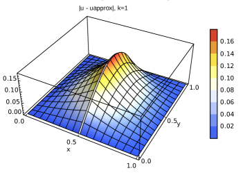
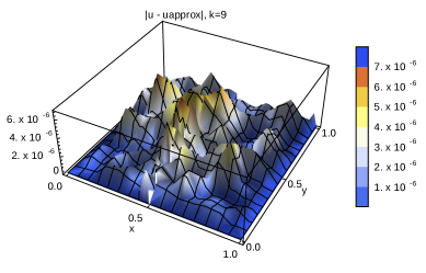
The numerical calculations were carried out using the program Wolfram Mathematica (see Figure 4). In computations the following Wolfram functions were used with the corresponding arguments: NDSolveValue (to assign the computed value to each component of the vector-function – the solution of the system of two equations with partial derivatives), DirichletCondition (to specify boundary values within the function NDSolveValue), Piecewise (to represent the solution on the whole area for further visualization), NMaxValue (to calculate uniform norm), Do (to organize the outer loop for iterations), along with other supplementary functions to calculate norms and get respective graphs.
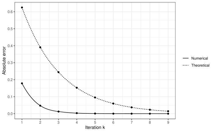
From the Theorem 3, we have $Q=q^{+}\sum_{j=1}^{m}\beta_{j}^{+}+q^{-}\sum_{i=1}^{n}\beta_{i}^{-}$, where $0<q^{+},q^{-}<1$. The absolute error decreases approximately as $O(Q^{k})$. Considering the nonlocal contact condition of the numerical example, $Q<5/8$.

Figure 5 compares the absolute error (in C-norm) with theoretical value $\left(\frac{5}{8}\right)^{k}$.

Refer to caption
Figure 5: Absolute error (numerical) and $Q^{k}$ versus iteration $k$
[Uncaptioned image]
Table 1: Relative error

Figures 7-7 show the behavior of relative error $\frac{\|u_{exact}-u_{appr}\|_{C}}{\|u_{exact}\|_{C}}$ (uniform C-norm is taken on the open area $D$) versus iteration $k$, for $k=1,\ldots,5$ and $k=6,\ldots,10$, respectively (see also results in Table 1).

Refer to caption
Figure 6: Relative error versus iteration k, k=1..5
Refer to caption
Figure 7: Relative error versus iteration k, k=6..10

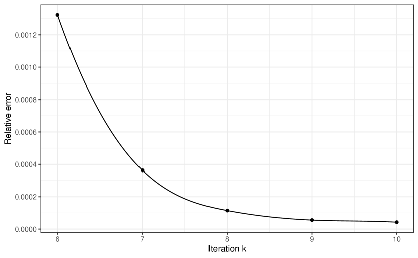
The results of numerical calculations fully agree with the theoretical conclusions and show the efficiency of the proposed iterative procedure.

5 Conclusion

The theory of contact problems is widely used in many fields of mechanics (including construction mechanics), in mechanical engineering, etc. In these problems, various contact conditions are considered along the contact line (see, for example, [23, 18]).

In the present article a new type of nonclassical boundary-value problem with nonlocal contact conditions along the contact line is considered for elliptic equation with variable coefficients and mixed derivatives. Thus, using the results of the present article, one can expand the class of contact problems.

The main results of the proposed article can be formulated as follows:

The existence and uniqueness of the solution of a nonlocal contact problem for the elliptic equation with variable coefficients and mixed derivatives is proved. For this aim the convergent iterative method (22)-(26) is constructed, which also is used to find the numerical solution. The method converges to the solution of the problem (16)-(19) at the rate of infinitely decreasing geometric progression. By using this iterative algorithm the solution of a non-classical contact problem is reduced to the solution of a sequence of classical boundary problems, which can be solved applying well-studied methods. The results of numerical calsulations agree with theoretical results.

The analytical solution in a form of series is received for the same problem, but with constant coefficients to avoid huge formulae. Moreover, the applied technique can be successfully used for more general problems, but in this case the use of spectral theory of linear operators will be needed.

In contrast to boundary nonlocal problems, convergence is achieved under the more general conditions: $0<\gamma^{-}+\gamma^{+}\leq 1$ (in the case of the Fourier method) and $0<\sum_{j=1}^{m}\beta_{j}^{+}+\sum_{j=1}^{n}\beta_{i}^{-}\leq 1$ (in the case of general equation with variable coefficients).

The technique used in the present article can also be applied for the problems with parabolic type equations.

6 Declarations

Availability of data and materials

Data sharing is not applicable to this article as no datasets were generated or analysed during the current study.

Competing interests

The authors declare that they have no competing interests.

Funding

This research received funding from the University of Malaga for its open access publication.

Authors’ contribution

All authors contributed to all sections. All authors read and approved the final manuscript.

Acknowledgements

Not applicable.

References

  • [1] A Ashyralyev and A Hamad, Numerical solution of the nonlocal boundary value problem for elliptic equations, Bulletin of the Karaganda University, Mathematics series 3 (2018), no. 91, 99–107.
  • [2] Richard Beals, Nonlocal elliptic boundary value problems, Bull. Amer. Math. Soc. 70 (1964), 693–696. MR 167700
  • [3] V Beridze, D Devadze, and H Meladze, On one nonlocal boundary value problem for quasilinear differential equations, Proceedings of A. Razmadze Mathematical Institute, vol. 165, 2014, pp. 31–39.
  • [4] Givi Berikelashvili, Nikolai I Ionkin, and Valentina A Morozova, On a nonlocal boundary-value problem for two-dimensional elliptic equation, Computational Methods in Applied Mathematics 3 (2001), no. 1, 62–71.
  • [5] Andrei Vasil’evich Bitsadze and Aleksander Andreevich Samarskii, Some elementary generalizations of linear elliptic boundary value problems, Doklady Akademii Nauk, vol. 185, Russian Academy of Sciences, 1969, pp. 739–740.
  • [6] Felix E Browder, Non-local elliptic boundary value problems, American Journal of Mathematics 86 (1964), no. 4, 735–750.
  • [7] J. R. Cannon, The solution of the heat equation subject to the specification of energy, Quart. Appl. Math. 21 (1963), 155–160. MR 160437
  • [8] Francisco Criado, Gamlet Meladze, and Nana Odisehlidze, An optimal control problem for Helmholtz equation with non-local boundary conditions and quadratic functional, Rev. R. Acad. Cienc. Exactas Fís. Nat. (Esp.) 91 (1997), no. 1, 65–69.
  • [9] T. Davitashvili and H. Meladze, Non-local contact problem for linear differential equations with partial derivatives of parabolic type with constant and variable coefficients, Lecture Notes of TICMI, vol. 22, 2021, p. 73–90.
  • [10] David Devadze, The existence of a generalized solution of an $m$-point nonlocal boundary value problem, Communications in Mathematics 25 (2017), no. 2, 159–169.
  • [11] Jesus Ildefonso Diaz and Jean-Michel Rakotoson, On a nonlocal stationary free-boundary problem arising in the confinement of a plasma in a stellarator geometry, Archive for Rational Mechanics and Analysis 134 (1996), no. 1, 53–95.
  • [12] Avner Friedman, Partial differential equations of parabolic type, Courier Dover Publications, 2008.
  • [13] D Gordeziani, N Gordeziani, and G Avalishvili, Nonlocal boundary value problems for some partial differential equations, Bull. Georgian Acad. Sci 157 (1998), no. 3, 365–368.
  • [14] D Gordeziani, H Meladze, and G Avalishvili, On one class of nonlocal in time problems for first-order evolution equations, Zhurnal Obchyslyuval’noı ta Prykladnoı Matematyky 88 (2003), no. 1, 66–78.
  • [15] David Gordeziani and Iulia Meladze, Nonlocal contact problem for two-dimensional linear elliptic equations, Bull. Georg. Natl. Acad. Sci 8 (2014), no. 1.
  • [16] Anatolii Konstantinovich Gushchin and VP Mikhaĭlov, On solvability of nonlocal problems for a second-order elliptic equation, Sbornik: Mathematics 81 (1995), no. 1, 101.
  • [17] Vladimir Aleksandrovich Il’in and Evgenii Ivanovich Moiseev, 2-d nonlocal boundary value problem for poisson’s operator in differential and difference variants, Matematicheskoe modelirovanie 2 (1990), no. 8, 139–156.
  • [18] KL Johnson, Contact mechanics, Cambridge University Press, Cambridge, 1985.
  • [19] L.V. Kantarovich and V.I. Krilov, Priblijonnie metodi visshego analiza (5-e izd.), m.-l., Fizmatlit, 1962, in Russian.
  • [20] A.P. Kartashev and B.L. Rozhdestvensky, Simple differential equations and introduction to variation calculus, Nauka, Moscow, 1986.
  • [21] Olga A. Ladyzhenskaya and Nina N. Ural’tseva, Linear and quasilinear elliptic equations, Academic Press, New York-London, 1968, Translated from the Russian by Scripta Technica, Inc, Translation editor: Leon Ehrenpreis. MR 0244627
  • [22] G. Lobjanidze, On non-classical solutions for some non-local bitsadze-samarski boundary value problem, Reports of Enlarged Sessions of the Seminar of I. Vekua Institute of Applied Mathematics, vol. 35, 2021, pp. 55–58.
  • [23] N. I. Muskhelishvili, Some basic problems of the mathematical theory of elasticity, english ed., Noordhoff International Publishing, Leiden, 1977. MR 0449125
  • [24] AM Nakhushev, Equations of mathematical biology, Vysshaya Shkola, Moscow (1995), 301.
  • [25] CV Pao, Reaction diffusion equations with nonlocal boundary and nonlocal initial conditions, Journal of mathematical analysis and applications 195 (1995), no. 3, 702–718.
  • [26] Ivan Georgievich Petrovsky, Lectures on partial differential equations, Courier Corporation, 2012.
  • [27] MP Sapagovas, Difference method of increased order of accuracy for the poisson equation with nonlocal conditions, Differential Equations 44 (2008), no. 7, 1018–1028.
  • [28] E. A. Volkov, A. A. Dosiyev, and S. C. Buranay, On the solution of a nonlocal problem, Comput. Math. Appl. 66 (2013), no. 3, 330–338.