:
\theoremsep
\jmlrproceedingsAABI 2024Workshop at the 6th Symposium on Advances in Approximate Bayesian Inference (non-archival), 2024
Warm Start Marginal Likelihood Optimisation
for Iterative Gaussian Processes
1 Introduction
Gaussian processes (Rasmussen and Williams, 2006) are a versatile probabilistic machine learning model that have found great success in many applications, such as Bayesian optimisation of black-box functions (Snoek et al., 2012) or data-efficient learning in robotics and control (Deisenroth et al., 2015). However, their effectiveness often depends on performing model selection, which amounts to finding good estimates of quantities such as kernel hyperparameters, and the amount of observation noise prescribed in the likelihood. For Gaussian processes, these quantities are typically learned by maximising the marginal likelihood of the training data, which balances the expressiveness and the complexity of a model in representing the training data. Unfortunately, conventional approaches which use the Cholesky factorisation have limited scalability, because the computational costs and memory requirements are respectively cubic and quadratic in the amount of training data.
Many methods have been developed to improve the scalability of Gaussian processes. Typically, they either leverage a handful of judiciously chosen inducing points to represent the training data sparsely; or solve large systems of linear equations using iterative methods. Sparse methods (Quiñonero-Candela and Rasmussen, 2005; Titsias, 2009; Hensman et al., 2013) are fundamentally limited in the number of inducing points, because the same cubic and quadratic scaling of compute and memory requirements still applies to the number of inducing points. With increasingly large or sufficiently complex data, a limited number of inducing points can no longer accurately represent the original data. In contrast, iterative methods (Gardner et al., 2018; Lin et al., 2023; Wu et al., 2024) attempt to solve the original problem up to a specified numerical precision, therefore allowing a trade-off between compute time and accuracy of a solution. Nonetheless, they can be slow in the large data regime due to slow convergence properties, sometimes requiring several days of training time despite leveraging parallel compute capabilities (Wang et al., 2019).
In this work, we consider marginal likelihood optimisation for iterative Gaussian processes. We introduce a three-level hierarchy of marginal likelihood optimisation for iterative Gaussian processes (Figure 2), and identify that the computational costs are dominated by solving sequential batches of large positive-definite systems of linear equations (Figure 3). We then propose to amortise computations by reusing solutions of linear system solvers as initialisations in the next step, providing a warm start. Finally, we discuss the necessary conditions and quantify the consequences of warm starts (Theorem 3.1) and demonstrate their effectiveness on regression tasks (Table 1), where warm starts achieve the same results as the conventional procedure while providing up to a average speed-up among datasets.
2 Gaussian Process Regression and Marginal Likelihood Optimisation
Formally, a Gaussian process is a stochastic process , such that, for any finite subset , the set of random variables follows a multivariate Gaussian distribution. In particular, is uniquely identified by a mean function and a positive-definite kernel function with kernel hyperparameters . We write to express that is a Gaussian process with mean and kernel .
For the purpose of Gaussian process regression, let the training data consist of inputs and corresponding targets . We consider the Bayesian model , where each identically and independently, and , where we assume without loss of generality. The posterior of this model is , with
| (1) | ||||
| (2) |
where , and refer to pairwise evaluations, resulting in a row vector, a column vector and a matrix respectively.
With and , the marginal likelihood as a function of and its gradient with respect to can be expressed as
| (3) | ||||
| (4) |
where the partial derivative of with respect to each element in is a matrix. If is small enough such that a Cholesky factorisation of is tractable then both and can be easily evaluated and used by any optimiser of choice to maximise . However, we are considering the case where is too large to compute the Cholesky factorisation of .
2.1 Marginal Likelihood Optimisation for Iterative Gaussian Processes
Marginal likelihood optimisation in iterative Gaussian processes can be structured into a three-level hierarchy (see Figure 2), as follows.
Iterative Optimiser
Typically, a first-order optimiser, such as Adam (Kingma and Ba, 2015), is used to maximise , which only requires estimates of , avoiding the evaluation of and . This allows us to focus on tractable estimates of .
Gradient Estimator
The gradient (4) involves two computationally expensive components: inverse matrix-vector products of the form and the trace term. The inverse matrix-vector products are readily approximated using iterative solvers to linear systems of the form . The trace term can also be reduced into inverse matrix-vector products using stochastic trace estimation, e.g. Hutchinson’s (Hutchinson, 1990), as follows
| (5) |
where probe vectors of length are introduced and is required for the estimator to be unbiased. Common choices for the distribution of are standard Gaussian, , or Rademacher, namely uniform random signs, . In theory, the latter exhibit lower estimator variance. Additionally, more advanced trace estimators have also been developed (Meyer et al., 2021; Epperly et al., 2024). However, in practice, standard Gaussian probes with Hutchinson’s trace estimator seem to work well.
Linear System Solver
After substituting the trace estimator into (4), the approximate gradient consists of terms that involve computing and by solving large systems of linear equations,
| (6) |
which share the same coefficient matrix . Because is positive-definite, the solution to the system of linear equations can also be obtained by finding the unique minimiser of the corresponding convex quadratic objective,
| (7) |
facilitating the use of iterative optimisers. In the context of Gaussian processes, conjugate gradients (Gardner et al., 2018; Wang et al., 2019; Wilson et al., 2020, 2021), alternating projections (Wu et al., 2024) and stochastic gradient descent (Lin et al., 2023, 2024) have been applied to optimise (7), serving as linear system solvers.
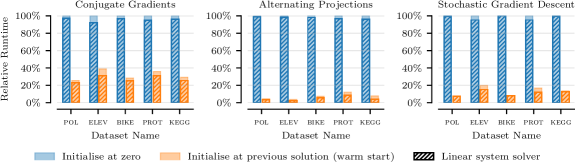
Notably, the linear system solver dominates the overall computational costs, such that reducing its runtime translates to substantial computational savings (see Figure 3). Therefore, we propose to amortise computations by reusing solutions of linear systems to initialise the linear system solver in the next marginal likelihood step, providing a warm start.
3 Warm Start Marginal Likelihood Optimisation
Given that the iterative linear system solver dominates the computational costs of marginal likelihood optimisation (see Figure 3), reducing the number of necessary solver iterations until convergence will translate to substantial computational savings. However, iterative solvers are typically initialised at zero for each gradient computation step, even though the hyperparameters do not change much between steps.111Notable exceptions are Artemev et al. (2021), who warm start in a sparse lower bound on , and Antorán et al. (2023), who warm start a stochastic gradient descent solver for generalised linear models. Therefore, we propose to amortise computational costs for any solver type by reusing solutions of previous linear systems to warm start (i.e. initialise) linear system solvers in the subsequent step.
At iterations and of the marginal likelihood optimiser, associated with and , the linear system solver must solve two batches of linear systems, namely
| (8) | ||||
| (9) |
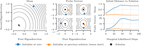
where and are related through the change from to and and are further related through sharing the same right-hand side in the linear system. In such a setting, where the coefficient matrix only changes slightly and the right-hand side remains fixed, we can approximate using a first-order Taylor expansion of ,
| (10) | ||||
| (11) |
If is small then will be close to (see Figure 1), such that we can reuse to initialise the linear system solver when solving for . To satisfy the condition of fixed right-hand sides, we propose to set at the cost of introducing some bias throughout optimisation, which can be bounded, as we will now quantify.
Theorem 3.1.
Let and be the marginal likelihood and its gradient as defined in (3) and (4) respectively, and let be an approximation to the gradient where the trace is approximated with fixed samples as in (5). Assume that the hyperparameter optimisation domain is convex, closed and bounded, and that is a conservative field. Then, given a sufficiently large number of samples , the hyperparameters obtained by maximising the objective implied by the approximate gradients will be -close in terms of the true objective to the true maximum of the objective ,
with probability at least .
See Appendix A for details. In practice, a small number of samples seems to be sufficient.
4 Experiments
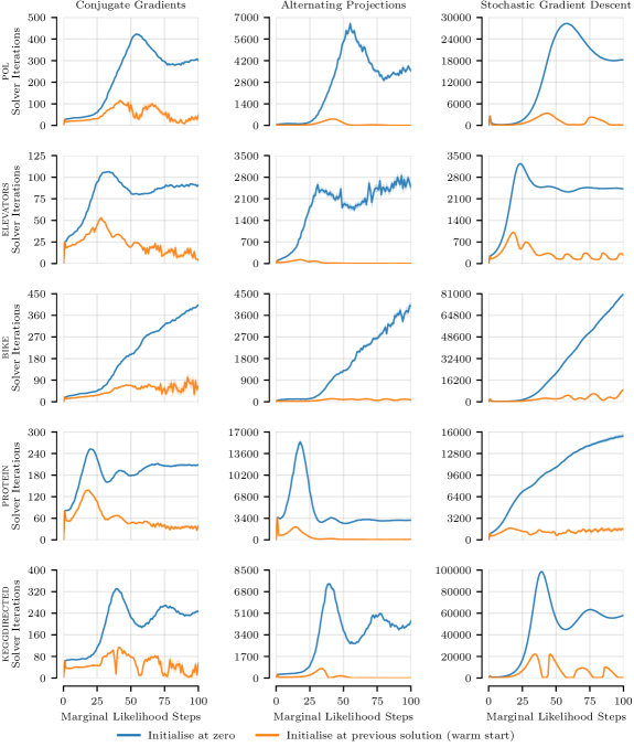
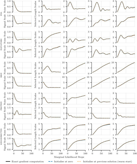
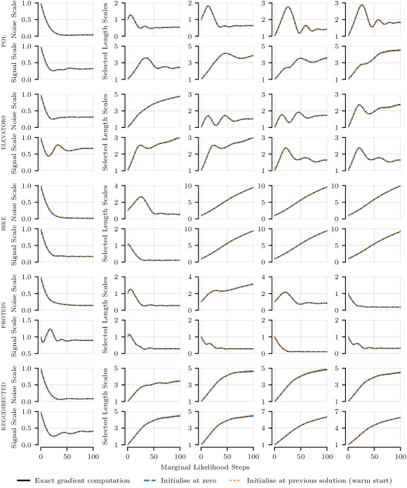
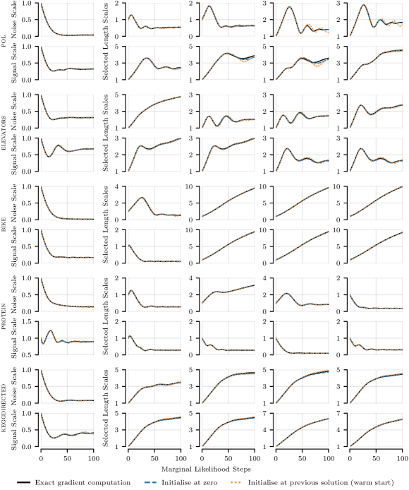
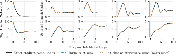
To investigate the effectiveness of warm starts, we performed marginal likelihood optimisation on five UCI regression datasets (Dua and Graff, 2017), comparing the procedure described in Section 2.1 with resampled probe vectors versus fixed probe vectors and warm starts. In particular, we used the Matérn- kernel with length scales per input dimension and a scalar signal scale. Observation noise, signal scale and length scales were initialised at and jointly optimised by performing 100 steps of Adam (Kingma and Ba, 2015) with a learning rate of 0.1, where the gradient was estimated using (5) with standard Gaussian probe vectors . We conducted experiments with different linear system solvers, namely conjugate gradients (Gardner et al., 2018; Wang et al., 2019), alternating projections (Wu et al., 2024) and stochastic gradient descent (Lin et al., 2023, 2024). See Appendix B for further implementation details.
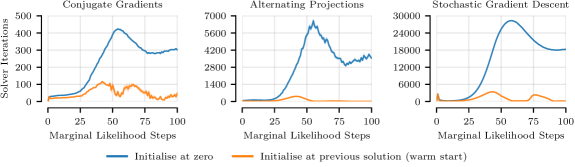
Figure 3 illustrates that warm starts significantly reduce the runtime of linear system solvers, and consequently the total runtime, being most effective for alternating projections. Figure 4 visualises that these speed-ups are due to substantial decreases in the number of linear system solver iterations required to reach a specified tolerance. Table 1 reports the final test log-likelihoods, computed using Cholesky factorisation, and total runtimes after 100 steps of marginal likelihood optimisation. Warm starts achieve the same test performance while providing an average speed-ups among datasets from to , showing that fixing probe vectors and reusing solutions does not impact performance in practice. Figure 5 shows that optimisation traces obtained using warm starts are almost identical to the traces obtained by resampling probe vectors and reinitialising at zero, and exact gradient computation using Cholesky factorisation. See Table 2 for more experimental results.
| Test Log-Likelihood | Total Runtime (min) | Average | |||||||||
|---|---|---|---|---|---|---|---|---|---|---|---|
| pol | elev | bike | prot | kegg | pol | elev | bike | prot | kegg | Speed-Up | |
| CG | 1.27 | -0.39 | 2.15 | -0.59 | 1.08 | 7.86 | 2.76 | 7.69 | 31.44 | 64.29 | — |
| + ws | 1.27 | -0.39 | 2.15 | -0.59 | 1.08 | 2.00 | 1.07 | 2.18 | 11.27 | 18.81 | 3.2 |
| AP | 1.27 | -0.39 | 2.15 | -0.59 | 1.08 | 22.39 | 13.55 | 12.31 | 45.42 | 62.24 | — |
| + ws | 1.27 | -0.39 | 2.15 | -0.59 | 1.08 | 0.99 | 0.52 | 0.90 | 5.52 | 4.86 | 16.7 |
| SGD | 1.27 | -0.39 | 2.18 | -0.59 | 1.08 | 41.31 | 4.92 | 81.84 | 46.92 | 360.44 | — |
| + ws | 1.27 | -0.39 | 2.15 | -0.59 | 1.07 | 3.08 | 0.98 | 6.73 | 7.87 | 48.72 | 8.8 |
5 Conclusion
We discussed marginal likelihood optimisation for iterative Gaussian processes and proposed warm starts to amortise linear system solver computation. We analysed the consequences of warm starts theoretically, and investigated their behaviour during hyperparameter optimisation on regression tasks empirically. Our experiments demonstrated that warm starts provide substantial reductions in computational costs, while maintaining predictive performance and matching optimisation traces of exact gradient computation using Cholesky factorisation.
Acknowledgments
Jihao Andreas Lin and Shreyas Padhy were supported by the University of Cambridge Harding Distinguished Postgraduate Scholars Programme. José Miguel Hernández-Lobato acknowledges support from a Turing AI Fellowship under grant EP/V023756/1. We thank Javier Antorán and Runa Eschenhagen for helpful discussions. This work was performed using resources provided by the Cambridge Service for Data Driven Discovery (CSD3) operated by the University of Cambridge Research Computing Service (www.csd3.cam.ac.uk), provided by Dell EMC and Intel using Tier-2 funding from the Engineering and Physical Sciences Research Council (capital grant EP/T022159/1), and DiRAC funding from the Science and Technology Facilities Council (www.dirac.ac.uk).
References
- Antorán et al. (2023) Javier Antorán, Shreyas Padhy, Riccardo Barbano, Eric T. Nalisnick, David Janz, and José Miguel Hernández-Lobato. Sampling-based inference for large linear models, with application to linearised Laplace. In International Conference on Learning Representations, 2023.
- Artemev et al. (2021) Artem Artemev, David R. Burt, and Mark van der Wilk. Tighter bounds on the log marginal likelihood of gaussian process regression using conjugate gradients. In International Conference on Machine Learning, 2021.
- Bradbury et al. (2018) James Bradbury, Roy Frostig, Peter Hawkins, Matthew James Johnson, Chris Leary, Dougal Maclaurin, George Necula, Adam Paszke, Jake VanderPlas, Skye Wanderman-Milne, and Qiao Zhang. JAX: composable transformations of Python+NumPy programs, 2018.
- Deisenroth et al. (2015) Marc Peter Deisenroth, Dieter Fox, and Carl Edward Rasmussen. Gaussian Processes for Data-Efficient Learning in Robotics and Control. IEEE Trans. Pattern Anal. Mach. Intell., 2015.
- Dua and Graff (2017) Dheeru Dua and Casey Graff. UCI Machine Learning Repository, 2017.
- Epperly et al. (2024) Ethan N. Epperly, Joel A. Tropp, and Robert J. Webber. XTrace: Making the Most of Every Sample in Stochastic Trace Estimation. Matrix Analysis and Applications, 45(1), 2024.
- Gardner et al. (2018) Jacob Gardner, Geoff Pleiss, Kilian Q Weinberger, David Bindel, and Andrew G Wilson. GPyTorch: Blackbox Matrix-matrix Gaussian Process Inference with GPU Acceleration. In Advances in Neural Information Processing Systems, 2018.
- Hensman et al. (2013) James Hensman, Nicolò Fusi, and Neil D Lawrence. Gaussian Processes for Big Data. In Uncertainty in Artificial Intelligence, 2013.
- Hutchinson (1990) M.F. Hutchinson. A stochastic estimator of the trace of the influence matrix for Laplacian smoothing splines. Communications in Statistics - Simulation and Computation, 19(2), 1990.
- Kingma and Ba (2015) Diederik P. Kingma and Jimmy Ba. Adam: A Method for Stochastic Optimization. In International Conference on Learning Representations, 2015.
- Lin et al. (2023) Jihao Andreas Lin, Javier Antorán, Shreyas Padhy, David Janz, José Miguel Hernández-Lobato, and Alexander Terenin. Sampling from Gaussian Process Posteriors using Stochastic Gradient Descent. In Preprint, arXiv:2306.11589, 2023.
- Lin et al. (2024) Jihao Andreas Lin, Shreyas Padhy, Javier Antorán, Austin Tripp, Alexander Terenin, Csaba Szepesvári, José Miguel Hernández-Lobato, and David Janz. Stochastic Gradient Descent for Gaussian Processes Done Right. In International Conference on Learning Representations, 2024.
- Meyer et al. (2021) Raphael Meyer, Cameron Musco, Christopher Musco, and David Woodruff. Hutch++: Optimal Stochastic Trace Estimation. Symposium on Simplicity in Algorithms, 2021, 2021.
- Quiñonero-Candela and Rasmussen (2005) Joaquin Quiñonero-Candela and Carl Edward Rasmussen. A Unifying View of Sparse Approximate Gaussian Process Regression. Journal of Machine Learning Research, 6, 2005.
- Rasmussen and Williams (2006) C. E. Rasmussen and C. K. I. Williams. Gaussian Processes for Machine Learning. MIT Press, 2006.
- Snoek et al. (2012) Jasper Snoek, Hugo Larochelle, and Ryan P. Adams. Practical Bayesian Optimization of Machine Learning Algorithms. In Advances in Neural Information Processing Systems, 2012.
- Titsias (2009) Michalis K Titsias. Variational learning of inducing variables in sparse Gaussian processes. In Artificial Intelligence and Statistics, 2009.
- Vershynin (2012) Roman Vershynin. Introduction to the non-asymptotic analysis of random matrices. In Compressed Sensing: Theory and Applications, 2012.
- Wang et al. (2019) Ke Alexander Wang, Geoff Pleiss, Jacob R. Gardner, Stephen Tyree, Kilian Q. Weinberger, and Andrew Gordon Wilson. Exact Gaussian Processes on a Million Data Points. In Advances in Neural Information Processing Systems, 2019.
- Wilson et al. (2020) James T. Wilson, Viacheslav Borovitskiy, Alexander Terenin, Peter Mostowsky, and Marc Peter Deisenroth. Efficiently Sampling Functions from Gaussian Process Posteriors. In International Conference on Machine Learning, 2020.
- Wilson et al. (2021) James T. Wilson, Viacheslav Borovitskiy, Alexander Terenin, Peter Mostowsky, and Marc Peter Deisenroth. Pathwise Conditioning of Gaussian Processes. Journal of Machine Learning Research, 22, 2021.
- Wu et al. (2024) Kaiwen Wu, Jonathan Wenger, Haydn Jones, Geoff Pleiss, and Jacob R. Gardner. Large-Scale Gaussian Processes via Alternating Projection. In International Conference on Artificial Intelligence and Statistics, 2024.
Appendix A Mathematical Derivations
Throughout this appendix, we will denote the number of data examples as , such that , and the number of samples in the trace estimator in (5) with . We will denote the optimisation domain for the hyperparameters as , where we assume . We will also assume that all elements in have finite fourth moments . For standard normal , we have , and for Rademacher we have . Furthermore, we assume that the coordinates of are also pairwise independent, which will again be the case for Gaussian or Rademacher random variables.
Theorem A.1.
Let , as in (4), and let be an approximation to with samples, as in (5). Assume that the absolute value of the eigenvalues of are upper-bounded on the domain of by and such that the eigenvalues of their product are upper-bounded by . Then, for any , if the number of samples is sufficiently large, we have
| (12) |
i.e. the -th component of the approximate gradient will be within distance of the true gradient on the entire optimisation space with probability at least for any .
Proof A.2.
Let be the eigendecomposition of , where and are two sets of orthonormal vectors. We will notationally suppress the dependence of on going forwards. First, we rewrite ,
| (13) | ||||
| (14) | ||||
| (15) | ||||
| (16) | ||||
| (17) | ||||
| (18) |
Therefore, we can bound the norm of the difference as
| (19) | ||||
| (20) |
where is the operator (spectral) norm of .
Lemma A.3.
, where is an -net on an -sphere .
Proof A.4.
We turn the lower bound on the spectral norm into a lower bound on for any which is a close approximation to the largest-norm eigenvalue eigenvector.
Consider the unit vector such that . Such a vector exists , because the supremum is taken over a compact subspace of . Note that if we have a unit vector such that , then
| (21) | |||||
| (22) | |||||
| (23) | |||||
| (24) | |||||
Consider a finite -net on the unit sphere . There exists such a collection with cardinality at most , and thus such a finite -net exists for . By (21), if , then for some we have that . Hence
| (25) | |||||
| (26) | |||||
| (27) | |||||
Lemma A.5.
For pairwise independent zero-mean identity-covariance with pairwise independent coordinates, and any unit vector
| (28) |
Proof A.6.
| (29) | |||
| (30) | |||
| (31) | |||
| (32) | |||
| (33) | |||
| (34) | |||
| (35) | |||
| (36) |
Therefore, the expectation of the above can be simplified as
| (37) | |||
| (38) | |||
| (39) |
The expectation in the terms of the first sum will be if : if then , and if then . Hence, for all non-zero terms and the first sum can be simplified as .
Then, we again have four cases for the terms :
| (40) |
and so, separating the sum into these cases, we get
| (41) | |||
| (42) | |||
| (43) | |||
| (44) | |||
| (45) |
Combining the previous lemmas gives:
Lemma A.7.
for as defined (13), for any , where is the fourth moment of the coordinates of .
Proof A.8.
Combining Lemmas A.5 and A.3, and noting that there exists an -net of size at most (Vershynin, 2012) yields the result.
Theorem A.1 implies a bound on the norm of the gradient error on the optimisation domain by a simple union bound over each coordinate of .
Theorem A.9.
Under the assumptions of Theorem A.1,
| (47) |
i.e. the approximate gradient will be within of the true gradient on the entire optimisation space with probability at least .
Now, if is a conservative field, and so is implicitly a gradient of some (approximate) objective , the above result allows us to bound the error on the solution found when optimising using the approximate gradient instead of the actual gradient . However, in general, need not be strictly conservative. In practice, since converges to a conservative field the more samples we take, we may assume that it is close enough to being conservative for the purposes of optimisation on hardware with finite numerical precision. Assuming that is conservative allows us to show the following bound on the optimum found when optimising using , which is a restatement of Theorem 3.1:
Theorem A.10.
Let and be defined as in Theorem A.1. Assume is a conservative field. Assume the optimisation domain is convex, closed and bounded. Then, given a sufficiently large number of samples s, a maximum obtained by maximising the objective implied by the approximate gradients will be -close in terms of the true objective to the true maximum of the objective :
| (48) |
with probability at least , where is the maximum distance between two elements in .
Proof A.11.
Let be an approximate objective implied by the gradient field , namely a scalar field such that . Such a scalar field exists if is a conservative field, and is unique up to a constant (which does not affect the optimum).
Assume that is sufficiently large such that the gradient difference is bounded by with probability at least . As per Theorem A.9, this will be the case when
| (49) |
For any two points , with , we have that
| (50) | |||
| (51) | |||
| (52) | |||
| (53) | |||
| (54) | |||
| (55) | |||
Hence,
| (57) | ||||
| (58) |
which gives the bound in the theorem.
Appendix B Implementation Details
Our implementation uses the JAX library (Bradbury et al., 2018) and all experiments were conducted on A100 GPUs using double floating point precision. The softplus function was used to enforce positive value constraints during hyperparameter optimisation. During each step of marginal likelihood optimisation, the linear system solvers were run until all linear systems in the batch reached a relative residual norm of less than for the linear system , corresponding to the mean, and for the linear systems , corresponding to the samples. Conjugate gradients and alternating projections keep track of the residual as part of the algorithm. For stochastic gradient descent, we estimate the current residual by keeping a residual vector in memory and updating it sparsely whenever we compute the gradient on a mini-batch of data, leveraging the property that the gradient is equal to the residual. In practice, we find that this estimates an approximate upper bound on the true residual. For conjugate gradients, we did not use any preconditioner. For alternating projections, we used a block size of 2000. For stochastic gradient descent, we used a mini-batch size of 1000, momentum of 0.9, no Polyak averaging, and learning rates of 90, 20, 100, 20, and 30 respectively for pol, elevators, bike, protein and keggdirected, which were selected by performing a grid search.
Appendix C Additional Empirical Results
| Test RMSE | Test LLH | Total Runtime | Solver Runtime | Speed-Up | ||
|---|---|---|---|---|---|---|
| pol , | CG | 0.075 0.001 | 1.268 0.008 | 7.857 0.111 | 7.641 0.110 | — |
| + ws | 0.075 0.001 | 1.268 0.009 | 2.003 0.027 | 1.790 0.026 | 3.9 | |
| AP | 0.075 0.001 | 1.269 0.008 | 22.390 0.331 | 22.158 0.326 | — | |
| + ws | 0.075 0.001 | 1.268 0.009 | 0.993 0.015 | 0.780 0.014 | 22.6 | |
| SGD | 0.075 0.001 | 1.266 0.010 | 41.306 0.201 | 41.215 0.201 | — | |
| + ws | 0.075 0.001 | 1.268 0.007 | 3.077 0.016 | 2.989 0.016 | 13.4 | |
| elevators , | CG | 0.355 0.003 | -0.386 0.007 | 2.758 0.044 | 2.542 0.042 | — |
| + ws | 0.355 0.003 | -0.386 0.007 | 1.072 0.014 | 0.858 0.012 | 2.6 | |
| AP | 0.355 0.003 | -0.386 0.007 | 13.547 0.345 | 13.331 0.344 | — | |
| + ws | 0.355 0.003 | -0.386 0.007 | 0.516 0.006 | 0.303 0.004 | 26.2 | |
| SGD | 0.355 0.003 | -0.385 0.007 | 4.921 0.069 | 4.685 0.015 | — | |
| + ws | 0.355 0.003 | -0.386 0.007 | 0.980 0.065 | 0.748 0.004 | 5.2 | |
| bike , | CG | 0.033 0.003 | 2.150 0.018 | 7.689 0.128 | 7.451 0.126 | — |
| + ws | 0.033 0.003 | 2.150 0.017 | 2.180 0.038 | 1.945 0.036 | 3.5 | |
| AP | 0.033 0.003 | 2.151 0.018 | 12.306 0.210 | 12.068 0.207 | — | |
| + ws | 0.033 0.003 | 2.153 0.018 | 0.904 0.014 | 0.670 0.012 | 13.6 | |
| SGD | 0.033 0.003 | 2.179 0.020 | 81.843 1.373 | 81.676 1.372 | — | |
| + ws | 0.032 0.003 | 2.149 0.031 | 6.733 0.168 | 6.567 0.168 | 12.2 | |
| protein , | CG | 0.503 0.004 | -0.587 0.010 | 31.438 0.476 | 29.850 0.458 | — |
| + ws | 0.503 0.004 | -0.588 0.010 | 11.270 0.156 | 9.685 0.138 | 2.8 | |
| AP | 0.503 0.004 | -0.587 0.010 | 45.417 0.622 | 43.829 0.607 | — | |
| + ws | 0.503 0.004 | -0.587 0.010 | 5.519 0.068 | 3.934 0.053 | 8.2 | |
| SGD | 0.504 0.004 | -0.587 0.010 | 46.915 0.350 | 44.661 0.349 | — | |
| + ws | 0.504 0.004 | -0.589 0.009 | 7.874 0.024 | 5.621 0.024 | 6.0 | |
| keggdirected , | CG | 0.084 0.002 | 1.082 0.017 | 64.290 0.768 | 61.902 0.760 | — |
| + ws | 0.084 0.002 | 1.081 0.017 | 18.807 0.228 | 16.415 0.220 | 3.4 | |
| AP | 0.084 0.002 | 1.082 0.017 | 62.235 0.625 | 59.848 0.618 | — | |
| + ws | 0.084 0.002 | 1.081 0.018 | 4.857 0.054 | 2.464 0.046 | 12.8 | |
| SGD | 0.084 0.002 | 1.081 0.019 | 360.436 4.079 | 357.734 4.076 | — | |
| + ws | 0.084 0.002 | 1.073 0.014 | 48.721 0.548 | 46.020 0.545 | 7.4 | |