Hybrid Multi-Head Physics-informed Neural Network for Depth Estimation in Terahertz Imaging

Abstract

Terahertz (THz) imaging is one of the hotspots in the field of optics, where the depth information retrieval is a key factor to restore the three-dimensional appearance of objects. Impressive results for depth extraction in visible and infrared wave range have been demonstrated through deep learning (DL). Among them, most DL methods are merely data-driven, lacking relevant physical priors, which thus request for a large amount of experimental data to train the DL models. However, large training data acquirement in the THz domain is challenging due to the requirements of environmental and system stability, as well as the time-consuming data acquisition process. To overcome this limitation, this paper incorporates a complete physical model representing the THz image formation process into traditional DL networks to retrieve the depth information of objects. The most significant advantage is the ability to use it without pre-training, thereby eliminating the need for tens of thousands of labeled data. Through experiments validation, we demonstrate that by providing diffraction patterns of planar objects with their upper and lower halves individually masked, the proposed physics-informed neural network (NN) can automatically optimize and, ultimately, reconstruct the depth of the object through interaction between the NN and a physical model. The obtained results represent the initial steps towards achieving fast holographic THz imaging using reference-free beams and low-cost power detection.

1 Introduction

THz radiation refers to electromagnetic radiation within the frequency range of approximately 0.1 THz to 10 THz, corresponding to wavelengths of 3 mm to 30 $\mu$m. THz imaging technology, as a promising direction in THz research, primarily benefits from the unique physical properties of this frequency band: firstly, it possesses strong penetration capability, enabling easy transmission through non-metallic and non-polar materials such as ceramics, plastics, and foam, which are commonly opaque to infrared light; secondly, THz waves exhibit low photon energy, thus avoiding harmful ionization effects; thirdly, many molecules display distinct absorption and dispersion characteristics in the THz frequency range, allowing the establishment of molecular fingerprint spectra for substance identification; Moreover, THz waves demonstrate high sensitivity to water, making them particularly suitable for analyzing material hydration levels [1, 2, 3]. Over the past two decades, advancements in electronics and photonics technologies have propelled the rapid development of THz imaging technology, expanding its application areas into fields such as non-destructive testing [4], quality monitoring [5], security screening [6, 7], biomedical imaging [8], and sensing for robotics and vehicle control [9], where it has achieved notable successes, demonstrating advantages unmatched by traditional imaging techniques.

Depth information plays a crucial role in THz imaging; however, due to the lack of suitable hardware, the construction of THz multi-pixel detector arrays poses challenges, making it difficult to achieve a million-pixel imaging array camera akin to those in the visible light domain [10]. Therefore, although there are well-established algorithms for depth restoration in the visible light domain [11], applying these algorithms to the terahertz domain remains quite challenging. At the current technological level, estimating depth in THz imaging primarily relies on several methods: focus measurement [12], time-of-flight [13], and heterodyne detection [14, 15]. Focus measurement techniques determine the distance of target objects by adjusting beam focusing, but this often requires multiple scans of the target, thus consuming considerable time and resources. Time-of-flight utilizes the propagation time of THz waves to estimate the distance to the object’s surface, but precision may be compromised in complex scenes or heavily occluded scenarios. Heterodyne detection involves mixing the transmitted signal from the object with a local reference signal to achieve distance estimation, but this requires a complex system and is susceptible to environmental noise and stray signals. Therefore, exploring more efficient methods for depth information acquisition is imperative for advancements in THz imaging technology.

Recently, DL techniques have emerged as promising and effective methods in the field of inverse problem [16, 17, 18], primarily relying on supervised deep learning approaches that utilize labeled experimental data [19, 20, 21]. Nevertheless, the expensive acquisition of THz images poses a challenge for supervised training with experimental data.

In this paper, we propose a novel hybrid multi-head physics-informed neural network (PINN) for depth estimation in THz holographic imaging. This method incorporates multi-input U-Net [22] with a physical prior knowledge, specifically, the angular spectrum theory [23, 24]. Hence, there is no need for thousands of labeled data to train the network. Instead, the model is trained with only two diffraction patterns, each with either the upper or lower portion masked, serving as inputs. The network weights and bias factors are then optimized through the interaction between the neural network and the physical model, ultimately yielding a feasible model solution that satisfies the imposed physical constraints.

2 Methods

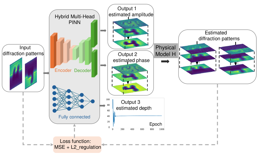
Figure 1: Schematic illustration of the pipeline of proposed depth estimation algorithm. The input of the neural network is the measured field amplitude diffraction pattern, each with half of the object masked separately. The output consists of estimated phase and amplitude maps, along with depth information for the object. Subsequently, these outputs are numerically propagated through the physical model $H$ to simulate the diffraction and measurement processes, generating the estimated diffraction patterns. MSE between the input patterns and estimated patterns, along with L2 regularization, serve as the loss function for optimizing the neural network parameters.

Figure 1 displays the proposed hybrid multi-head PINN algorithm, demonstrated using handwritten digits as an example. Note that no pre-training on large labeled datasets is required. The network solely relies on two diffraction patterns as input, each obtained by masking the upper or lower halves of the object and propagating the transmitted waves over a distance $d$. The first output of the PINN is for generating the estimated amplitude, while the second is for the estimated phase of the imaged objects. The two output paths share the CNN’s down-sampling layers and part of the up-sampling layers to ensure that the same object information is analyzed, which is inspired by U-Net [25] structure. At the last layer, these two paths separate from each other (see Appendix A for details). The third output of the PINN predicts the value for the depth, evaluated through a fully connected network structure. In our scenario, the amplitude within the masked metal area theoretically becomes 0, while the phase is randomized as long as it can reveal contours. For simplification of computation, we set the phase within the masked metal area to be 0 as well. Subsequently, the physical model $H$ is applied to convert network outputs into estimated diffraction patterns. The mean squared error (MSE) between inputs (the actual diffraction patterns) and estimated diffraction patterns, coupled with L2 regularization, guides the network’s optimization of weights and biases via gradient descent. In image processing, MSE is commonly used to measure the quality of the reconstructed image compared to the ground truth. It represents the Euclidean distance between images and is simple and efficient to evaluate, making it suitable for large-scale image processing tasks. Additionally, MSE is a convex function and possesses good mathematical properties [26]. The L2 regularization [27] aims to constrain the model’s complexity by incorporating weight decay, thereby enhancing the model’s generalization ability and mitigating overfitting. This loss function ensures the convergence of calculated diffraction patterns to input patterns via the iteration process. Through iterations, simultaneous searches for amplitude, phase, and depth information converge toward consistent feasible solutions. Notably, since all parameters in the physical model $H$ are considered, the proposed algorithm is universally applicable to holographic systems, irrespective of whether they involve phase objects or not.

As mentioned, the physical model, $H$, simulates the experimental THz imaging process. If a planar object is illuminated by a collimated beam, the complex-valued field amplitude immediately behind the object can be written as

$$E_{0}(x,y,z=0)=A_{0}(x,y,0)e^{i\phi_{0}(x,y;0)},$$ (1)

where $A_{0}$ and $\phi_{0}$ are the amplitude and the phase of the transmission rate of the object. Over a distance $d$, diffraction reshapes the field to [23]

$$E_{d}(x,y,z=d)=\iint\hat{E}_{0}(f_{x},f_{y})\,G\,e^{i2\pi(f_{x}x+f_{y}y)}df_{x}\,df_{y},$$ (2)

where $G=e^{ikd\sqrt{1-\lambda^{2}f_{x}^{2}-\lambda^{2}f_{y}^{2}}}$ is the wave propagation function, $\lambda$ is the wavelength, $\hat{E}_{0}$ is the spatial Fourier transform of $E_{0}$ with $f_{x}=x/\lambda d$ and $f_{y}=y/\lambda d$ as the spatial frequencies in the $x$ and $y$ directions. The diffraction pattern is the field’s absolute value

$$A(x,y,z=d)=\left|E_{d}(x,y,z=d)\right|=H(\phi_{0},A_{0},d),$$ (3)

where $H$ represents the mapping function relating the object to the diffraction pattern $A$.

For a conventional fitting, other than with PINNs, one usually attempts to learn a mapping function $R_{\theta}$ ($\theta$ denoting the network weights and bias parameters) from a large number of labeled data $(A_{k},d_{k})$, the labeled training set $S_{T}={(A_{k},d_{k}),k=1,2,...,K}$.

$$R_{\theta^{*}}=\mathop{\arg\min}_{\theta}\|R_{\theta}(A_{k})-d_{k}\|^{2}\qquad\forall(d_{k},A_{k})\in S_{T}.$$ (4)

Instead, in the PINN proposed here, the loss function is formulated by combining the physical model $H$ and the network output $R_{\theta}$ as

$$loss=\|H(R_{\theta}(A(x,y;d)))-A(x,y;d)\|^{2}+\lambda\sum_{i=1}^{m}\theta^{2}$$ (5)

where the diffraction pattern $A_{d}$ is the input of the NN. The regularization term $\lambda\sum_{i=1}^{m}\theta^{2}$ is defined as the Euclidean norm or L2 norm of the weight matrix, which is the sum of all squared weight values of the weight matrix. Here, we set the value of $\lambda$ to 0.01. In this way, the PINN optimization is solved with gradient descent with the above objective

$$\theta^{*}=\mathop{\arg\min}_{\theta}(loss)$$ (6)

When the optimization is complete, the resulting mapping function can then be used to reconstruct the depth with its third output:

$$\tilde{d}=R_{\theta^{*}}(A(x,y;d))$$ (7)

3 Results and discussion

We demonstrate the performance of the proposed method using data derived from simulations (THz-emulated MNIST) and experiments, respectively.

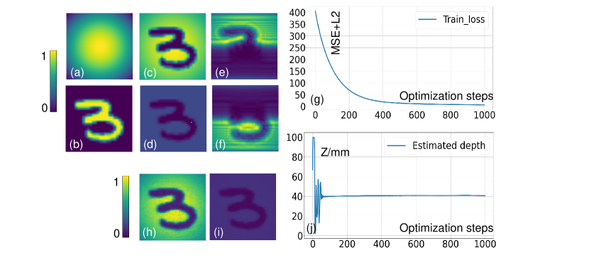
Figure 2: Simulation results in the ideal situation. (a) represents an ideal Gaussian distribution; (b) is a digit from the MNIST dataset; (c) and (d) are the ground truth of the amplitude and phase of the object; (e) (f) are the diffraction patterns of the digit diffracted at a distance $d=40\;mm$ with either its upper or lower half masked; (g) is the loss function curve during the training process; (h) and (i) are the predicted amplitude and phase after training for 1000 epochs; (j) is the optimization curve of the depth.

In our simulation, we assume an ideal scenario where there exists an uniform Gaussian beam without noise interference. Fig 2(a) depicts the ideal Gaussian intensity profile, with its phase being uniformly distributed. Fig 2(b) presents a digit three from the MNIST dataset, serving as an example. Depending on the material (with dielectric information such as refractive index) and thickness we intend to set, we can obtain the ground truth of the object’s amplitude and phase on the object plane, as shown in Fig 2(c) and (d). Fig 2(e) and (f) illustrate the diffraction patterns at a distance $d=40\;mm$ when respectively occluding the upper and lower halves of the digit, which serve as inputs to our network. The loss function, depicted in Fig 2(g), shows a continuous decrease with increasing iterations, stabilizing around 1.25 after 800 epochs, indicating the network has been sufficiently optimized. At this point, the network’s outputs include the estimated amplitudes (Fig 2(h)) and phases (Fig 2(i)). As iterations progress, the predicted depth gradually converges to a stable value of 40.01 mm in this example after around 200 epochs. It can be observed that in ideal conditions, the network’s predictions for depth are highly accurate.

We then compare our proposed method with a combination method consisting of back-propagation and shape from focus (SFF) [28], as well as the supervised DL method in the following.

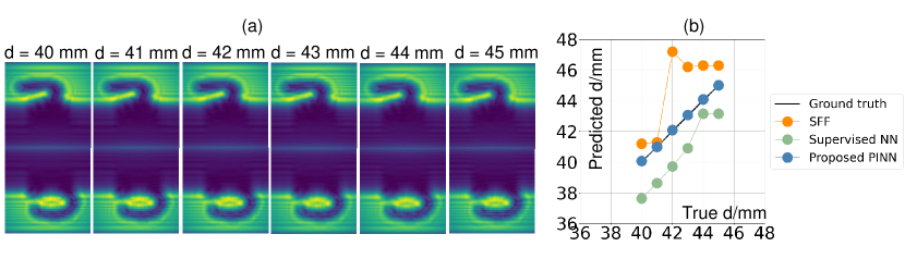
Figure 3: Diffraction patterns and comparison of our proposed PINN, supervised NN and back-propagation with SFF at diffraction distances ranging from 40 mm to 45 mm.

It is evident that at a minute diffraction distance difference of 1 mm, the differences in diffraction patterns are imperceptible to the naked eye, as shown in Fig 3(a). Hence, extracting depth information from such patterns is nontrivial and remarkably valuable. Fig 3(b) displays the comparison of our proposed PINN, supervised NN and back-propagation with SFF at diffraction distances ranging from 40 mm to 45 mm. The orange line represents the results of backpropagation combined with SFF (see Appendix B for specific sharpness curves). Its error is significant, approaching approximately 5 mm at some points compared to the ground truth. It is worth noting that during backpropagation, only the amplitude is utilized as input. Setting the phase to the same value as the amplitude yields superior results compared to setting it to 1, hence here it is set to the amplitude value. The green line represents the predictions of the supervised NN, which performs slightly better than backpropagation combined with SFF. However, at 45 mm and 46 mm, its predictions are identical. This is because in preparing the training dataset, it is impractical to cover all possible depth positions, resulting in potential information gaps at certain depths. Currently, our supervised network utilizes 60,000 pairs of training datasets and 10,000 pairs of testing datasets. Theoretically, its predictive performance can improve with further data augmentation. The blue line illustrates the predictions of our proposed hybrid multi-head PINN method, which agrees well with the ground truth (the black line), significantly outperforming the other two methods. Moreover, this method doesn’t require time-consuming pre-training like supervised learning.

We further utilize the coefficient of determination ($R^{2}$) to evaluate the performance of depth estimation out of the three methods. The $R^{2}$ can be calculated as follows:

$$R^{2}=1-\frac{SS_{res}}{SS_{tot}}$$ (8)

where $SS_{res}$ is the sum of squares of residuals, and $SS_{tot}$ is the total sum of squares. Generally, the closer $R^{2}$ is to 1, the better the model performs in the prediction. The $R^{2}$ values for the backpropagation with SFF method, the supervised learning method, and our method are -1.6168, -0.4291, and 0.9986, respectively.

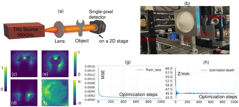
Figure 4: Experimental set-up and results in realistic situation. (a) and (b) display a schematic of the THz holographic imaging system and a photograph of our setup. (c) (d) show the diffraction patterns we measured. (e) and (f) are estimated amplitude and phase, respectively. (g) displays the loss curve during the training process. (h) is the optimization curve of the depth estimation, where the ground truth is $d=45\;mm$.

To validate the proposed methods by experiments, we performed THz measurements at 300 GHz. The schematic diagram and experimental photographs are shown in Fig. 4 (a) and (b). One can see that this is actually a single-beam lens-less imaging geometry. The illuminating radiation from a 300-GHz THz source is collimated by a focusing lens, with a 10-cm focal length and 4-inch aperture. The lens has a homemade hyperboloidal-planar shape. The NA of the lens allows to illuminate the objects over their full extension with a collimated Gaussian beam, free from beam modulations caused by diffraction at the lens edge.

To acquire the diffraction pattern, we placed the THz single-pixel TeraFET detector [29] at a distance $d=45\;mm$ from the object, on a 2D translation stage to scan and record the diffraction patterns. The radiation enters the detector chip from the back-side, passing a Si substrate lens with a diameter of 4 mm[30, 31]. The recorded two diffraction patterns are shown in Fig. 4(c) and (d). The object is a wrench with a thickness of 1 mm. The size of the object is around $30$ mm $\times$ $60$ mm, and the scanned image area is 80$\times$80 pixels with a 1-mm² pixel pitch.

In realistic scenarios, unlike the ideal case where a uniform Gaussian beam is assumed as discussed earlier, there may be non-uniform distributed noise present. We first utilize heterodyne detection to measure the amplitude and phase of the reference THz beam, with each system requiring only one measurement (details can be found in Appendix C). The amplitude and phase of the reference beam serve as prior information fed into our PINN. We use the sigmoid activation function to ensure that the amplitude and phase output to be between 0 and 1, then multiply them by the reference to get the final amplitude and phase predictions. Fig. 4 (g) illustrates the loss curve of our network, showing that after 500 iterations the network’s loss stabilizes at a value of 0.000085. It is worth noting that, unlike the ideal case, we use loss in Eq.5 without L2 here because the noise is non-Gaussian. This also speeds up the convergence of the network, indicating that there is only a 0.000085 mean squared error between the actual diffraction patterns (input) and the diffraction patterns predicted by the integration of the network and physical model $H$’s evaluation. Fig. 4 (e) and (f) depict the network’s output, amplitude and phase, respectively. Fig. 4 (h) shows the depth estimation from the network as a function of the optimization steps (iterations). Clearly we see that the network quickly predicts the correct depth information ($d=45\;mm$) and stabilizes around the ground truth value. We also employed a combination of backpropagation and SFF along with supervised learning methods for a comparison. However, both of these approaches showed an inability to accurately predict actual experimental data.

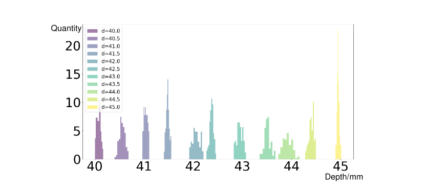
Figure 5: Resolution of our proposed PINN at diffraction distances ranging from 40 mm to 45 mm.

Given that our method can accurately predict depth information with minimal errors in both ideal and realistic scenarios, we proceeded to determine the resolution of this approach. According to the theory of phase detection, the depth resolution can be quantified as[32]:

$$\sigma_{d}=4\gamma\frac{\lambda d^{3}}{D^{3}}.$$ (9)

When the phase difference between pixels on objects is 0, $\gamma$ equals 1.64. Here, $D$ represents the lens aperture (in our experiments, it is 80mm), $\lambda$ denotes the wavelength, and $d$ represents the distance from the object to the detector. Therefore, in our system, the theoretical resolution can be determined to be around 0.82 - 1.17 mm. This resolution still requires the simultaneous use of both the diffracted amplitude and phase of the object. We used diffraction patterns from 40 mm to 45 mm, with intervals of 0.5 mm, totaling 11 distances, as inputs to the proposed PINN for resolution evaluation. To demonstrate robustness, we conducted 500 predictions for each distance. Fig. 5 illustrates the histogram of the predicted depth results for each distance, where the horizontal axis represents the depths and the vertical axis represents the histogram of counts for PINN predictions over each single depth. It can be observed that the PINN can accurately predict diffraction patterns with roughly 0.5 mm intervals, and its resolution can even be better than 0.5 mm.

4 Conclusions

In conclusion, we have developed a novel physics-informed deep learning method for predicting the depth of planar objects using only two diffraction patterns obtained by masking the upper and lower halves of the object. In contrast to supervised learning methods that require large training datasets to optimize their weights and biases, and optical approaches involving backpropagation and SFF, our method offers more accurate and stable predictions in both ideal and realistic scenarios. Additionally, our investigation into the resolution of depth reconstruction reveals that our method can achieve a resolution of 0.5 mm or even better, surpassing the ideal resolution that requires additional object phase information for depth reconstruction. Therefore, our hybrid multi-head physics-informed neural network significantly advances the depth estimation for planar objects in the THz holographic systems, marking a crucial step forward in THz 3D imaging.

Appendix A

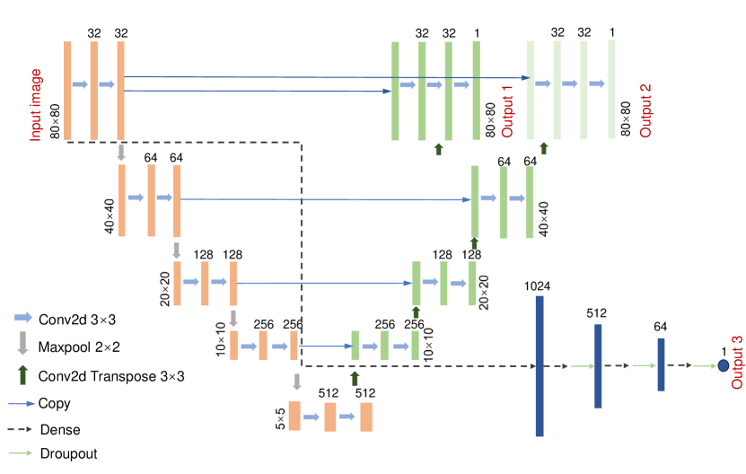
Figure 6: Structure of the proposed hybrid multi-head PINN

The architecture of the proposed PINN as employed for the supervised DL method is implemented using TensorFlow, an open-source deep-learning software package [33]. We use TensorFlow version 1.9.0 and Python 3.6.5. We adopt the estimation (Adam) [34] with a learning rate of 0.0005 to optimize the weights and biases. We add uniformly distributed noise between 0 and $\frac{1}{30}$ to the fixed input diffraction pattern in every optimization step to achieve better convergence. As shown in Fig. 6, each encoding step contains two 3$\times$3 convolutional layers (blue arrows) with Relu activation function and one 2$\times$2 max pooling layer (grey arrows), while each decoding process contains one 3$\times$3 deconvolutional layer (dark-green arrows), one concat layer to increase the dimension of the feature [35] (thin blue arrows), and two convolutional layers. In addition, there are three consecutive fully connected layers (dash black arrows) and dropout layers (green arrows) for depth prediction. The size of the input image is 80$\times$80 pixels. The network usually needs 1000 epochs to find an excellent estimation. This takes  10 min on a PC with a sixteen-core 3.50-GHz CPU and a 64-GB RAM, using Nvidia GeForce RTX 3080 GPU.

Appendix B

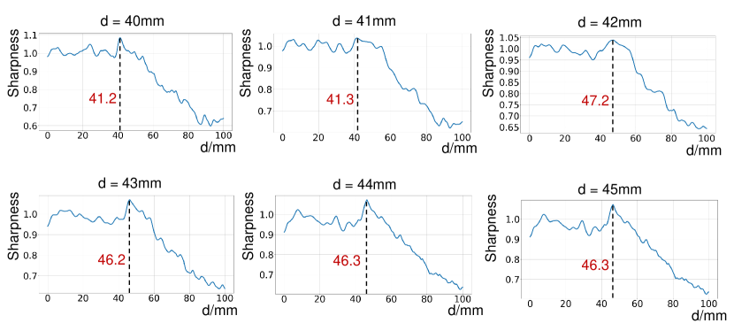
Figure 7: SFF results at diffraction distance of 40mm - 45mm

Figure 7 illustrates the sharpness curve using the SFF algorithm. The SFF algorithm uses the sum of the modified Laplacian (ML) operator described in [36] on each pixel of all the images to calculate the focus versus the optical axis. Then, a focus measure at the pixel $(x,y,z)$ is calculated by:

$$F(x,y,z)=\sum_{X=x-N}^{x+N}\sum_{Y=y-N}^{y+N}ML(X,Y,z)\quad if\,ML>T$$ (10)

$N$ determines the window size to compute the focus measure. $T$ is a threshold value to remove the contribution of the too-low contrasted region of the images. The depth position is found by the sharpest / maximum value as $d=z|_{max(F(x,y,z)}$). A more accurate method to find the best focus consists of an interpolation of $F$ along $z$ axis, considering a Gaussian distribution, also described in [36]:

$$F(x,y,z)=F_{p}(x,y)e^{-\frac{1}{2}(\frac{z-\overline{d}(x,y)}{\sigma})^{2}}$$ (11)

With $F_{p}$, the new maximum focusing value, and $\overline{d}$ the new best focusing z position. $\sigma$ is the depth of field of the terahertz imaging system, considered constant all over the image area.

Appendix C

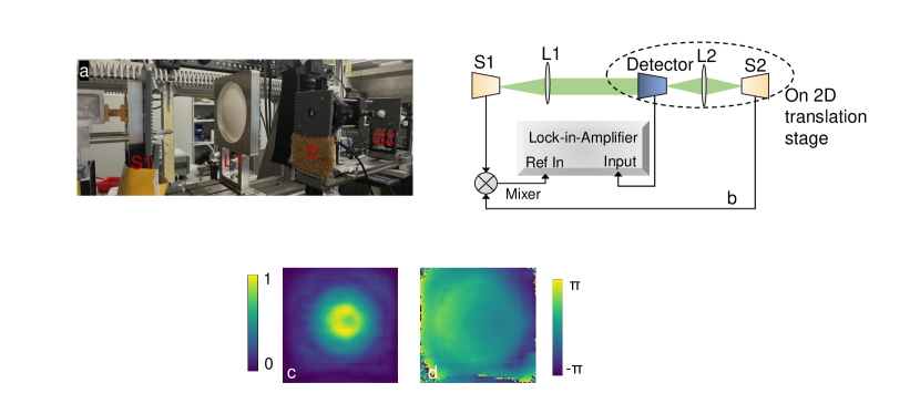
Figure 8: Experimental heterodyne setup and detected reference images. (a) and (b) display a photograph and a schematic of the THz holographic imaging system with heterodyne detection. (c) and (d) visualize the amplitude and phase images recorded by the heterodyne detection system.

A photograph and a schematic of the experimental heterodyne setup are shown in Fig. 8(a), (b). We use this setup to obatin the ground truths. The system [14, 37] contains two frequency-locked 300-GHz electrical multiplier chains (S1, S2) with a 18-kHz frequency offset between them. One (S2) is used as a local oscillator (LO) and the other (S1) provides the object-illuminating wave. The LO wave is focused onto the detector directly by a biconvex focusing lens, L2, with a 5-cm focal length and 2-inch aperture. The illuminating radiation is collimated by a focusing lens, L1, with a 10-cm focal length and 4-inch aperture. L1 is an aspheric lens. Given the required large NA, its hyperboloidal-planar shape avoids the spherical aberrations which one would encounter if a spherical lens would have been used. The NA of L1 has to be large enough to guarantee that the objects are illuminated over their full extension with a collimated Gaussian beam free of beam modulations arising by diffraction at the edge of the lens. Such modulations introduce high-spatial-frequency signatures which can make the learning process difficult. Furthermore, the alignment of the lens is also crucial, since the phase is sensitive to optical-axis displacements. Fig. 8 (c) and (d) show amplitude and phase maps of the beam, demonstrating that the beam has an isotropic amplitude distribution and near-constant phase over its cross-section. A numerical evaluation of the beam profile reveals a Gaussian-like beam shape. The bluish horizontal segments in Fig. 8(d) result from position shift errors induced by forward- and backward-scanning of the translation stage. This effect is not visible in the amplitude map because the amplitude is insensitive to slight variations of the scanner position. This also proves that our algorithm has no strict requirements for the calibration of the reference beam and can be used in a simple way.

References

- [1] X.-C. Zhang, J. Xu, et al., Introduction to THz wave photonics, Vol. 29, Springer, 2010.
- [2] A. Redo-Sanchez, X.-C. Zhang, Terahertz science and technology trends, IEEE Journal of Selected topics in quantum electronics 14 (2) (2008) 260–269.
-
[3]
A. Y. Pawar, D. D. Sonawane, K. B. Erande, D. V. Derle, Terahertz technology and its applications, Drug Invention Today 5 (2) (2013) 157–163.
doi:https://doi.org/10.1016/j.dit.2013.03.009.
URL https://www.sciencedirect.com/science/article/pii/S0975761913000264 - [4] I. Amenabar, F. Lopez, A. Mendikute, In introductory review to thz non-destructive testing of composite mater, Journal of Infrared, Millimeter, and Terahertz Waves 34 (2) (2013) 152–169.
- [5] F. Ellrich, M. Bauer, N. Schreiner, A. Keil, T. Pfeiffer, J. Klier, S. Weber, J. Jonuscheit, F. Friederich, D. Molter, Terahertz quality inspection for automotive and aviation industries, Journal of Infrared, Millimeter, and Terahertz Waves 41 (4) (2020) 470–489.
-
[6]
J. F. Federici, B. Schulkin, F. Huang, D. Gary, R. Barat, F. Oliveira, D. Zimdars, THz imaging and sensing for security applications—explosives, weapons and drugs, Semiconductor Science and Technology 20 (7) (2005) S266–S280.
doi:10.1088/0268-1242/20/7/018.
URL https://doi.org/10.1088/0268-1242/20/7/018 - [7] F. Friederich, W. von Spiegel, M. Bauer, F. Z. Meng, M. D. Thomson, S. Boppel, A. Lisauskas, B. Hils, V. Krozer, A. Keil, T. Löffler, R. Henneberger, A. K. Huhn, G. Spickermann, P. H. Bolívar, H. G. Roskos, Thz active imaging systems with real-time capabilities, IEEE Transactions on Terahertz Science and Technology 1 (2011) 183–200.
- [8] X. Yang, X. Zhao, K. Yang, Y. Liu, Y. Liu, W. Fu, Y. Luo, Biomedical applications of terahertz spectroscopy and imaging, Trends in Biotechnology 34 (10) (2016) 810–824.
- [9] D. Jasteh, M. Gashinova, E. Hoare, T.-Y. Tran, N. Clarke, M. Cherniakov, Low-thz imaging radar for outdoor applications, in: 2015 16th International Radar Symposium (IRS), IEEE, 2015, pp. 203–208.
- [10] A. Rogalski, F. Sizov, Terahertz detectors and focal plane arrays, Opto-electronics review 19 (3) (2011) 346–404.
- [11] Z.-Q. Zhao, P. Zheng, S.-T. Xu, X. Wu, Object detection with deep learning: A review, IEEE Transactions on Neural Networks and Learning Systems 30 (11) (2019) 3212–3232. doi:10.1109/TNNLS.2018.2876865.
- [12] J.-B. Perraud, J.-P. Guillet, O. Redon, M. Hamdi, F. Simoens, P. Mounaix, Shape-from-focus for real-time terahertz 3d imaging, Optics letters 44 (3) (2019) 483–486.
- [13] H. S. Kim, J. Kim, Y. H. Ahn, Terahertz nondestructive time-of-flight imaging with a large depth range, Current Optics and Photonics 6 (6) (2022) 619–626.
- [14] H. Yuan, D. Voss, A. Lisaukas, D. Mundy, H. G. Roskos, 3D Fourier imaging based on 2D heterodyne detection at THz frequencies, APL Photonics 4 (10) (2019) 106108. doi:10.1063/1.5116553.
- [15] H. Yuan, A. Lisauskas, M. D. Thomson, H. G. Roskos, 600-GHz Fourier imaging based on heterodyne detection at the 2nd sub-harmonic, Optics Express 31 (24) (2023) 40856–40870. doi:10.1364/OE.487888.
- [16] L.-G. Pang, K. Zhou, N. Su, H. Petersen, H. Stöcker, X.-N. Wang, An equation-of-state-meter of quantum chromodynamics transition from deep learning, Nature Commun. 9 (1) (2018) 210. arXiv:1612.04262, doi:10.1038/s41467-017-02726-3.
- [17] S. Shi, K. Zhou, J. Zhao, S. Mukherjee, P. Zhuang, Heavy quark potential in the quark-gluon plasma: Deep neural network meets lattice quantum chromodynamics, Phys. Rev. D 105 (1) (2022) 014017. arXiv:2105.07862, doi:10.1103/PhysRevD.105.014017.
- [18] L. Wang, S. Shi, K. Zhou, Reconstructing spectral functions via automatic differentiation, Phys. Rev. D 106 (5) (2022) L051502. arXiv:2111.14760, doi:10.1103/PhysRevD.106.L051502.
- [19] L. Boominathan, M. Maniparambil, H. Gupta, R. Baburajan, K. Mitra, Phase retrieval for Fourier ptychography under varying amount of measurements, arXiv:1805.03593 (2018).
- [20] M. Deng, S. Li, A. Goy, I. Kang, G. Barbastathis, Learning to synthesize: robust phase retrieval at low photon counts, Light: Science & Applications 9 (1) (2020) 1–16.
- [21] G. Ju, X. Qi, H. Ma, C. Yan, Feature-based phase retrieval wavefront sensing approach using machine learning, Optics Express 26 (24) (2018) 31767–31783.
- [22] O. Ronneberger, P. Fischer, T. Brox, U-net: Convolutional networks for biomedical image segmentation, in: Medical image computing and computer-assisted intervention–MICCAI 2015: 18th international conference, Munich, Germany, October 5-9, 2015, proceedings, part III 18, Springer, 2015, pp. 234–241.
- [23] J. W. Goodman, Introduction to Fourier optics, Roberts and Company publishers, 2005.
- [24] M. J. Xiang, H. Yuan, L. X. Wang, K. Zhou, H. G. Roskos, Amplitude/phase retrieval for terahertz holography with supervised and unsupervised physics-informed deep learning, IEEE Transactions on Terahertz Science and Technology 14 (2) (2024) 208–215. doi:10.1109/TTHZ.2024.3349482.
- [25] L. Alzubaidi, J. Zhang, A. J. Humaidi, A. Al-Dujaili, Y. Duan, O. Al-Shamma, J. Santamaría, M. A. Fadhel, M. Al-Amidie, L. Farhan, Review of deep learning: Concepts, cnn architectures, challenges, applications, future directions, Journal of Big Data 8 (1) (2021) 1–74.
- [26] Z. Wang, A. C. Bovik, Mean squared error: Love it or leave it? a new look at signal fidelity measures, IEEE Signal Processing Magazine 26 (1) (2009) 98–117. doi:10.1109/MSP.2008.930649.
- [27] C. Cortes, M. Mohri, A. Rostamizadeh, L2 regularization for learning kernels, arXiv preprint arXiv:1205.2653 (2012).
-
[28]
J.-B. Perraud, J.-P. Guillet, O. Redon, M. Hamdi, F. Simoens, P. Mounaix, Shape-from-focus for real-time terahertz 3d imaging, Opt. Lett. 44 (3) (2019) 483–486.
doi:10.1364/OL.44.000483.
URL https://opg.optica.org/ol/abstract.cfm?URI=ol-44-3-483 - [29] K. Ikamas, D. Čibiraitė, A. Lisauskas, M. Bauer, V. Krozer, H. G. Roskos, Broadband terahertz power detectors based on 90-nm silicon CMOS transistors with flat responsivity up to 2.2 THz, IEEE Electron Device Letters 39 (2018) 1413–1416.
- [30] H. Yuan, A. Lisaukas, M. Zhang, A. Rennings, D. Erni, H. G. Roskos, Dynamic-range enhancement of heterodyne THz imaging by the use of a soft paraffin-wax substrate lens on the detector, in: 2019 Photonics & Electromagnetics Research Symposium - Fall (PIERS - Fall), 2019, pp. 2607–2611. doi:10.1109/PIERS-Fall48861.2019.9021735.
- [31] H. Yuan, A. Lisaukas, M. Zhang, Q. ul Islam, D. Erni, H. G. Roskos, Fourier imaging based on sub-harmonic detection at 600 GHz, in: 2022 Fifth International Workshop on Mobile Terahertz Systems (IWMTS), 2022, pp. 1–1. doi:10.1109/IWMTS54901.2022.9832459.
- [32] H. Yuan, Investigations on terahertz imaging based on coherent Fourier-space spectrum detection, doctoralthesis, Universitätsbibliothek Johann Christian Senckenberg (2023). doi:10.21248/gups.72276.
- [33] M. Abadi, P. Barham, J. Chen, Z. Chen, A. Davis, J. Dean, M. Devin, S. Ghemawat, G. Irving, M. Isard, et al., TensorFlow: a system for Large-Scale machine learning, in: 12th USENIX symposium on operating systems design and implementation (OSDI 16), 2016, pp. 265–283.
- [34] D. P. Kingma, J. Ba, Adam: A method for stochastic optimization, arXiv preprint arXiv:1412.6980 (2014).
- [35] S. Bell, C. L. Zitnick, K. Bala, R. Girshick, Inside-outside net: Detecting objects in context with skip pooling and recurrent neural networks, in: Proceedings of the IEEE conference on computer vision and pattern recognition, 2016, pp. 2874–2883.
- [36] S. K. Nayar, Y. Nakagawa, Shape from focus, IEEE Transactions on Pattern analysis and machine intelligence 16 (8) (1994) 824–831.
- [37] H. Yuan, A. Lisaukas, H. G. Roskos, THz Fourier imaging based on sub-harmonic heterodyne detection, in: 2020 45th International Conference on Infrared, Millimeter, and Terahertz Waves (IRMMW-THz), 2020, pp. 1–1. doi:10.1109/IRMMW-THz46771.2020.9370667.