- SHM
- structural health monitoring
- DIC
- digital image correlation
- ESPI
- electronic speckle pattern interferometry
- PDE
- partial differential equation
- MCMC
- Markov chain Monte Carlo
- probability density function
- NLS
- nonlinear least-squares
- ANN
- artificial neural network
- FFNN
- feed-forward neural network
- PINN
- physics-informed neural network
- FE
- finite element
- FEM
- finite element method
- BC
- boundary condition
- NLS-FEM
- nonlinear least-squares finite element method
- VFM
- virtual fields method
- RE
- relative error
- MAE
- mean absolute error
- relative norm
- RD
- relative deviation
- ARE
- absolute relative error
- SEM
- standard error of the mean
- GPU
- graphics processing unit
[1]\fnmDavid \surAnton
1]\orgdivInstitute for Computational Modeling in Civil Engineering, \orgnameTechnische Universität Braunschweig, \orgaddress\streetPockelsstraße 3, \cityBraunschweig, \postcode38106, \countryGermany
2]\orgdivInstitute of Applied Mechanics, \orgnameClausthal University of Technology, \orgaddress\streetAdolph-Roemer-Straße 2A, \cityClausthal-Zellerfeld, \postcode38678, \countryGermany
3]\orgdivInstitute for Acoustics and Dynamics, \orgnameTechnische Universität Braunschweig, \orgaddress\streetLanger Kamp 19, \cityBraunschweig, \postcode38106, \countryGermany
4]\orgdivComputational Mechanics Group, \orgnameEidgenössische Technische Hochschule Zürich, \orgaddress\streetTannenstrasse 3, \cityZürich, \postcode8092, \countrySwitzerland
Deterministic and statistical calibration of constitutive models from full-field data with parametric physics-informed neural networks
Abstract
The calibration of constitutive models from full-field data has recently gained increasing interest due to improvements in full-field measurement capabilities. In addition to the experimental characterization of novel materials, continuous structural health monitoring is another application that is of great interest. However, monitoring is usually associated with severe time constraints, difficult to meet with standard numerical approaches. Therefore, parametric physics-informed neural networks for constitutive model calibration from full-field displacement data are investigated. In an offline stage, a parametric PINN can be trained to learn a parameterized solution of the underlying partial differential equation. In the subsequent online stage, the parametric PINN then acts as a surrogate for the parameters-to-state map in calibration. We test the proposed approach for the deterministic least-squares calibration of a linear elastic as well as a hyperelastic constitutive model from noisy synthetic displacement data. We further carry out Markov chain Monte Carlo-based Bayesian inference to quantify the uncertainty. A proper statistical evaluation of the results underlines the high accuracy of the deterministic calibration and that the estimated uncertainty is valid. Finally, we consider experimental data and show that the results are in good agreement with a Finite Element Method-based calibration. Due to the fast evaluation of PINNs, calibration can be performed in near real-time. This advantage is particularly evident in many-query applications such as Markov chain Monte Carlo-based Bayesian inference.
keywords:
model calibration, parametric physics-informed neural networks, uncertainty quantification, solid mechanics1 Introduction
The calibration of constitutive models is a major research field in computational as well as experimental solid mechanics and has a wide range of applications in practice. The interest in appropriate methods for constitutive model calibration recently increased further with the improvement of full-field measurement capabilities and the associated increase in available full-field displacement data. Probably the most obvious application in the context of experimental solid mechanics is the characterization of novel materials from experimental data. Another application that is gaining increasing interest is continuous structural health monitoring (SHM) [1, 2]. Material parameters directly reflect the resistance to external impacts and indicate damage and material degradation and thus provide crucial information for the assessment of existing structures. Since in SHM stress data is typically not accessible, the material parameters of interest must be identified from displacement or strain data, measured by, e.g., digital image correlation (DIC) [3] or electronic speckle pattern interferometry (ESPI) [4], respectively.
The connection between constitutive model parameters and the measured full-field data is then established by the inverse solution of the parametric mechanical model. Traditionally, this inverse problem is solved by numerical methods, such as the nonlinear least-squares finite element method (NLS-FEM), see, for instance, [5, 6], or the virtual fields method (VFM) [7, 8]. While both NLS-FEM and VFM are well established in experimental mechanics, their application in SHM is oftentimes prohibitive since their computational costs do not meet the severe time constraints in online applications. Thus, there is great interest in methods that are suitable for repeated calibration in the laboratory or in online applications.
Recently, it has been shown that physics-informed neural networks (PINNs) [9] are particularly suited for solving inverse problems. \AcpPINN are a framework for solving forward and inverse problems involving nonlinear partial differential equations from the field of physics-informed machine learning [10]. The idea behind this method goes back to the 1990s [11, 12], but it became applicable only recently due to developments in automatic differentiation [13], software frameworks, such as TensorFlow [14] and PyTorch [15], and more powerful hardware. The main advantages of PINNs are a straightforward inclusion of training data and their use as a continuous ansatz function. Thanks to the latter, all quantities can be computed directly on the sensor locations, bypassing the need for interpolation as, e.g., in finite element method (FEM)-based calibration approaches.
In general, most numerical methods for calibrating constitutive models from full-field data can be classified into reduced and all-at-once approaches, see [16] for a recent review. Therein, an unifying framework for model calibration in computational solid mechanics has been developed. The reduced approach assumes that a parameters-to-state map exists, which is provided, e.g., by a PINN or a finite element (FE) simulation. In contrast, in the all-at-once approach, the state and the model parameters are inferred simultaneously. For PINNs as well as other numerical methods, it is possible to formulate the calibration problem both in the reduced as well as in the all-at-once setting.
In the literature, most contributions focusing on parameter identification with PINNs are associated with the all-at-once approach. Such formulations are also referred to as inverse PINNs. In [17, 18, 19, 20, 21, 22], inverse PINNs have been applied to parameter identification from full-field displacement data. However, many of the assumptions made therein do not match the conditions of real-world applications. This mainly concerns the magnitude and quality of the measured displacements. Some references, such as [20], even consider the availability of full-field stress data for identification, which in practice must be considered as unknown. In earlier work, some of the authors have further developed inverse PINNs towards parameter identification in a realistic regime [23], both concerning the magnitude of the material parameters as well as the noise level of the displacement data. Nevertheless, a severe restriction of inverse PINNs remains. In principle, they must be trained from scratch each time new measurements become available. This involves high computational costs and is a significant disadvantage when it comes to repeated online calibration or standardized material tests, where the setup basically remains the same.
In this contribution, we therefore focus on PINNs in a reduced approach. In an offline stage, the PINN is trained to learn a parameterized solution of the underlying parametric partial differential equation within a predefined range of material parameters. For this purpose, the material parameters are considered as additional inputs to the PINN, such that the predicted displacement no longer depends on the spatial position only, but also on the material parameters. To speed up the training process and to make it more robust, we suggest to include some data in the training process. This data may be generated by high-fidelity FE simulations. In the subsequent online stage, the pre-trained PINN then acts as a surrogate for the parameters-to-state map in calibration. This special variant of PINNs, known as parametric PINNs, have already been deployed for thermal analysis of a laser powder bed fusion process [24], magnetostatic problems [25], or for the optimization of an airfoil geometry [26]. To the best of our knowledge, parametric PINNs have not yet been used for the calibration of constitutive models in solid mechanics using real-world experimental data. Building up on our results reported in [16], we statistically evaluate the accuracy of the parametric PINNs for the calibration of constitutive models from noisy synthetic full-field data, extend the study to hyperelastic materials and consider experimental data.
We demonstrate that the parametric PINN approach enables an accurate and efficient model calibration and uncertainty quantification of the inferred material parameters in online applications, even though up to forward model evaluations are required. To illustrate this, we first consider the constitutive models for both small strain linear elasticity and finite strain hyperelasticity and perform a re-identification of the material parameters from noisy synthetic displacement data. In the deterministic setting, a nonlinear least-squares (NLS) problem is solved. A statistical evaluation of the results shows that the point estimates obtained by solving the NLS problem deviate only marginally from the true material parameters. We further treat the material parameters as random variables, conduct Bayesian statistical inference and quantify the uncertainty in the estimated material parameters. The posterior distribution of the material parameters is determined by carrying out a Markov chain Monte Carlo (MCMC) analysis. In order to validate the quantified uncertainty from a frequentist point of view, we perform a coverage test. The results for the statistical calibration show that the estimated uncertainties are also valid. In addition to the synthetic data, we calibrate the constitutive model for small strain linear elasticity using experimental full-field displacement data obtained from a tensile test. We demonstrate that the calibration with a parametric PINN shows good results compared to using FEM for both the deterministic as well as the statistical setting.
In summary, the advantages of using parametric PINNs as surrogates of the parameters-to-state map in the context of constitutive model calibration are:
-
•
Parametric PINNs allow for a near real-time calibration. Once a PINN has been trained in the offline stage, the evaluation of the parameters-to-state map in the online stage is very cheap. This is a clear advantage, especially when used in many-query approaches such as the deterministic NLS approach or the statistical MCMC analysis.
-
•
Parametric PINNs are continuous ansatz functions. No interpolation between the sensor locations and the numerical discretization is required for calibration.
- •
To support the advantages mentioned above and to increase the acceptance of parametric PINNs in the context of constitutive model calibration, the present study aims towards the following key contributions:
- •
-
•
We perform a statistical evaluation of the numerical results. To validate the estimated uncertainty in the Bayesian statistical setting from a frequentist point of view, we perform a coverage test.
-
•
We consider real-world experimental displacement data. We calibrate a linear elastic constitutive model using experimental data measured in a tensile test.
To the best of the authors knowledge, the above mentioned contributions in connection with parametric PINNs have not yet been considered in the literature.
The code for our numerical tests including the data generation, the training and validation of parametric PINNs as well as the calibration methods is implemented in the Python programming language. The PINN implementation is mainly based on the PyTorch framework [15]. The code for the FE data generation is built on top of the FEniCSx project [29]. Our research code is open source and available both on GitHub and Zenodo [30]. In addition, we also published the experimental data set on Zenodo [31].
The remainder of this paper is structured as follows: In Section 2, the balance of linear momentum and the considered constitutive models are recapitulated. We then provide a brief introduction to artificial neural networks and parametric PINNs in Section 3. In this section, we also elaborate on normalization steps necessary for real-world applications. In Section 4, the calibration problem both in the deterministic as well as the Bayesian statistical setting are formulated. Subsequently, in Section 5 and Section 6, we provide the results for our numerical tests including both synthetic and experimental full-field data, respectively. Finally, we conclude our investigations with a critical discussion and point out possible directions of future work in Section 7.
2 Solid mechanics preliminaries
The relationship between the measured displacements of a body and the material parameters is defined by the framework of solid mechanics. In the following, we briefly recapitulate the balance of linear momentum and elaborate on the constitutive models for both small strain linear elasticity and finite strain hyperelasticity. For a more in-depth introduction to solid mechanics, the reader is referred to standard text books, e.g., [32, 33].
2.1 Fundamental equations
The displacement of a material point in the undeformed reference configuration (denoted by subscript ) is defined by
| (1) |
where the vector corresponds to the position of a material point in the deformed configuration at time and represents the motion. In the following, the explicit time dependence is omitted for brevity. Furthermore, both the undeformed reference configuration and the deformed configuration are modeled as a subset of the physical Euclidean space with orthonormal basis vectors. Then, can be identified with the common three-dimensional vector space . More information on the geometrical treatment of continuum mechanics can be found in [34, 35].
In the reference configuration , the balance of linear momentum in its strong form and in static equilibrium states
| (2) |
Here, denotes the divergence operator with respect to the coordinates and represents the first Piola-Kirchhoff stress tensor. The density in the reference configuration is denoted by and are accelerations caused, for instance, by gravity. Equation 2 needs to be satisfied for all points inside the domain . The stress depends on the displacement via the strains and is parameterized by a set of material parameters . The semicolon indicates parameterization of in .
The PDE 2 is complemented by a set of Dirichlet and Neumann boundary conditions
| (3a) | ||||
| (3b) | ||||
with and denoting the complementary surfaces of the boundary , where denotes the closure of , with . Furthermore, and are the prescribed displacements and tractions on the boundaries, respectively, and is the normal vector on the outer surface of the reference configuration.
The system of equations arising from 2–3 is closed by the kinematics and a constitutive model describing the stress state as a function of strain, parameterized in the material parameters . In the following, we briefly recall the kinematics and constitutive equations for linear elasticity and hyperelasticity.
2.2 Linear elasticity
For linear, isotropic elasticity and small strains, the constitutive model states
| (4) |
where is the Cauchy stress tensor, is the second-order identity tensor and tr is the trace operator. Note that in the linear elastic theory, it is assumed that in 2–3. The linear strain tensor is defined as
| (5) |
where the gradient is defined with respect to the coordinates . Here, is assumed. Furthermore, denotes the deviatoric part of . The constitutive model is parameterized in material parameters composed of the bulk modulus and the shear modulus .
2.3 Hyperelasticity
In the following, we consider finite strains and compressible, isotropic hyperelastic materials. The first Piola-Kirchhoff stress tensor can be derived from a strain energy density function expressed in terms of the tensor-valued measure by
| (6) |
The deformation gradient and the right Cauchy-Green tensor are defined as
| (7) |
where is again the second-order identity tensor.
The strain energy density function can be additively decomposed into a volumetric and an isochoric part and , respectively:
| (8) |
Here, is the determinant of the deformation gradient and is the isochoric right Cauchy-Green tensor. There are many concurrent approaches to model the volumetric part . A common approach frequently stated in standard text books [32, 33] is to consider
| (9) |
where is again the bulk modulus. For the isochoric part , a Neo-Hookean-type ansatz
| (10) |
with the first invariant is chosen, where defines the shear modulus in the small strain limit.
The relation between and might lead to a non-physical behavior for large compressive and tensile states, see, for a discussion, [36, 37]. Thus, both the relation between and as well as the amount of the deformation has to be considered carefully. Again, as in the case of linear elasticity, the material parameters can be summarized as .
3 Parametric physics-informed neural networks
PINNs are a deep learning framework for solving forward and inverse problems involving PDEs, in which ANNs act as a global ansatz function to the PDE solution [9]. An extension of the ANN with additional inputs makes it even possible to learn parameterized forward solutions of PDEs. We first review the basics of ANNs. Subsequently, we lay emphasize on the key characteristic of parametric PINNs which is the formulation of the loss function. We further elaborate on necessary normalization steps for an application of the proposed parametric PINN formulation in a real-world setting.
3.1 Artificial neural networks
ANN are parameterized, nonlinear function compositions which serve as an approximation for an input-output mapping. There are several different formulations of this mapping, such as convolutional and recurrent neural networks. In the following, however, we restrict ourselves to fully-connected feed-forward neural networks. For a more in-depth introduction to ANNs, the reader is referred to standard text books, e.g., [38].
We consider a fully-connected FFNN composed of layers that defines a mapping from an input space to an output space in the general form
| (11) | ||||
where denotes the input vector, the output vector and the composition operator, such that ). Accordingly, the first layer and the last layer are the input and the output layer, respectively, and defined as
| (12) |
The layers between the input and the output layer are usually called hidden layers. The vector-valued output of the hidden layers and the output layer are defined as
| (13) |
Here, denotes the result of an affine transformation of the output vector of the downstream layer controlled by the matrix and the bias vector . The output of the hidden layers is computed by applying a nonlinear activation function on top of the affine transformation . In the output layer , the identity function is used as activation, such that
| (14) |
where is the identity matrix of size and is the size of the vector which is equivalent to the number of neurons in this layer. In this contribution, we use the hyperbolic tangent as activation functions in the hidden layers.
The weight matrices and bias vectors comprise the trainable parameters of the layers . All parameters of the FFNN can be combined in a single parameter vector with
| (15) |
Taking the trainable parameters into account, in the following, the FFNN defined by 11, 12, 13, 14 and 15 is denoted by . This notation highlights that the FFNN output does not only depend on the input but is also parameterized in the current realization of .
An appropriate point estimate of the parameters can be found by solving an optimization problem, often referred to as training of the ANN. The objective of the optimization problem is to minimize a loss function that provides a measure for the deviation of the ANN from the hidden input-output mapping. According to the universal function approximation theorem, any Borel measurable function can be approximated by an ANN with enough parameters with only mild assumptions on the activation function [39, 40, 41]. However, it should be noted that the issue of finding the optimal parameters of the ANN is still an open question and highly problem dependent.
3.2 Parametric physics-informed neural network formulation
Parametric PINNs are an extension of standard PINNs for learning parameterized forward solutions involving parametric PDEs. A parameterized ansatz is used to approximate the solution which is realized by an ANN with additional inputs besides the spatial coordinates. In the following, we apply parametric PINNs for solving the model 2–3 parameterized in the material parameters . We start by defining our ansatz function for the displacement field and the resulting discretized model. Subsequently, we formulate the loss function and elaborate on the training process.
First, we approximate the displacement field by the parametric ansatz
| (16) |
which acts as a function approximator to the solution of 2–3. Here, is a modified FFNN , whereby the modifications are explained later on. It should be noted that both the spatial coordinates and the material parameters are inputs to the ansatz . The FFNN is parameterized by the weights and biases as defined in 15. Furthermore, in this work, we consider the calibration from full-field displacement data as a two-dimensional problem and thus where is the number of material parameters.
In particular, we use an ansatz for the displacement field that differs from a standard FFNN as follows: We choose an ansatz function that strictly fulfills the Dirichlet boundary conditions 3a by construction, which is referred to as hard boundary conditions. Alternatively, the Dirichlet boundary conditions can be imposed by a separate loss term. This approach is referred to as soft boundary conditions. With the application of the hard boundary condition according to [42], the FFNN modifies to
| (17) |
where denotes an intermediate step in the derivation of the parameterized ansatz . Moreover, is a smooth extension of the boundary data and is a smooth distance function giving the distance of to the boundary . The vector is the summarized FFNN input vector. When selecting the distance function, it is important to ensure that vanishes on the boundary . It should be noted that and are vector valued functions of the same dimension as the ansatz output and that in 17 denotes the element-wise Hadamard multiplication operator, such that for two vectors . In this contribution, we use a normalized linear distance function defined as
| (18) |
where and are vectors containing the minimum and maximum coordinates for each dimension within , respectively. In addition, is a vector that contains the position of the Dirichlet boundary condition in the respective dimension. The element-wise Hadamard division operator is defined as for two vectors . Note that the distance function defined in 18 assumes that there is only one Dirichlet boundary condition in each dimension and that the Dirichlet boundaries are parallel to the Cartesian coordinate system. In general, however, hard boundary conditions can also be applied to complex geometries, as shown in [42].
Furthermore, we normalize the inputs and outputs of the ansatz because it is well known that this accelerates the convergence of the training of ANNs. According to [43], the mean value of each input feature should be close to zero. Since we assume that the input is evenly distributed over the input domain, we normalize the input by the following linear transformation
| (19) |
which maps the entries of the real input vector to the range . Here, and are vectors containing the minimum and maximum input features, respectively, and is a vector of ones. In addition, we normalize the ansatz outputs. Depending on the problem, the scales of the displacements can vary significantly in the different dimensions, as, e.g., in uniaxial tensile tests. At the same time, error metrics like the mean squared error are scale-sensitive. To give the displacement field approximation the same relative importance in all dimensions during training, we enforce the ansatz outputs to be also in the range . Therefore, we renormalize the output in a last step by another linear transformation
| (20) |
where is the intermediate normalized ansatz with its outputs enforced to be in the range . The vectors and contain the minimum and maximum expected displacements of the material body resulting from the range of material parameters under consideration, respectively. The intermediate normalized ansatz is defined as
| (21) |
In order to guarantee that the renormalized ansatz output still strictly fulfills the Dirichlet boundary conditions, the boundary extension in 21 must also be normalized by the inverse of 20 which is given by
| (22) |
Note that the input to in 21 is also normalized by definition 18.
Applying the normalization and renormalization steps from equations 18, 19, 20, 21 and 22 to the modified ansatz from equation 17, we finally obtain the ansatz
| (23) |
The normalization steps aim to condition the optimization problem that arises during PINN training. While the required minimum and maximum input values are given from the training data, the required minimum and maximum output values can, e.g., be extracted from given experimental or simulation data or be estimated based on prior knowledge such as boundary conditions. It is important to emphasize that at any time during training and prediction, only the non-normalized, extended inputs are fed into the ansatz. Likewise, the ansatz always outputs non-normalized displacements. This also means that the physics is not violated when the outputs are derived with respect to the inputs during training.
For the following steps, we reformulate the governing equations introduced in Section 2 as a function of the displacement state vector and the material parameters and define the discretized model
| (24) |
A statically and kinematically admissible displacement field must fulfill everywhere in . With PINNs, however, the displacement is only evaluated at discrete points, represented in the state vector . The latter comprises the displacement state vectors , and , where , and are the number of evaluation points inside the domain and on the Dirichlet and Neumann boundaries and , respectively. Accordingly, comprises , and . Furthermore, and are the vectors with the prescribed displacements and tractions, respectively. The implementation of the discrete model 24 for solving the forward problem using PINNs is introduced in the following.
Second, we define the loss function. The loss function encoding the physics in the model 24 and enhanced by data is defined as
| (25) |
The loss terms , and penalize the mean squared error of the approximation defined in 23 with respect to the PDE, the Neumann boundary condition and the data, respectively, and are defined as
| (26a) | ||||
| (26b) | ||||
| (26c) | ||||
where denotes the squared -norm. The training data consists of three sets , and :
-
(i)
is referred to as a set of collocation points sampled from the domain .
-
(ii)
consists of collocation points on the Neumann boundary with the prescribed tractions .
-
(iii)
contains points where the displacements can be obtained from, e.g., FE simulations.
The individual loss terms in 25 can additionally be weighted by , and to balance them. The weight factors may also be adapted during training, see, for instance, [44]. In order to calculate the partial derivatives required to evaluate the loss terms 26a–26b, the displacement field in the constitutive models 4 and 6 is approximated by the ansatz 16. The derivatives of the ansatz outputs with respect to the inputs are calculated using automatic differentiation [13]. If required, the loss function 25 may be complemented by further, problem specific loss terms, such as symmetry boundary conditions.
It should be noted that the loss function 25 does not contain a separate loss term for the Dirichlet boundary condition since we use a hard boundary condition for this, see 23. Provided that the stress is also considered as an output of the ANN in addition to the displacement, the Neumann boundary condition can in principle also be replaced by a hard boundary condition. In this work, we do not use hard Neumann boundary conditions, as we achieved high accuracy without them and do not observe any problems with the weak imposition of the Neumann boundary conditions.
Third, we optimize the ANN parameters . The optimization problem for finding an appropriate point estimate for the ANN parameters is defined as
| (27) |
and is usually carried out using gradient-based optimization algorithms, such as ADAM [45] or L-BFGS [46, 47, 48, 49, 50]. The required gradients of the loss function with respect to the ANN parameters can again be calculated by automatic differentiation. It should be noted, that the implementation of in 25 is not identical to the model formulation 24. However, implies that . Squaring the residuals in ensures that positive and negative deviations do not cancel out each other. In addition, larger residuals are penalized more than smaller residuals.
4 Constitutive model calibration
In this contribution, we formulate the calibration from full-field displacement data according to the reduced approach. Following the general problem statement, we elaborate on the deterministic nonlinear least-squares method. Afterwards, we address the calibration problem from a Bayesian statistical point of view. In both the deterministic as well as the Bayesian statistical setting, the parametric PINN is used as a surrogate for the mechanical model.
4.1 Deterministic calibration
General problem statement: Recalling the notation from Sections 2–3, the problem of constitutive model calibration is governed by the following set of equations
| (28) |
with state vector , full-field displacement data , material parameter vector and observation operator .
The latter relates the model state to the measurement data , such that . In principle, the observation operator can take many forms and may also account for indirectly measured quantities, such as strains. If full-field displacement measurements are available, it interpolates the model state to the sensor locations . These are the points where the displacement is measured. It is worth recalling that the PINN is a global ansatz function that can be evaluated directly at the sensor locations. Consequently, the observation operator becomes the identity operator, i.e., , where is the identity matrix of size . Hence, possible interpolation errors are avoided.
Solution approach: As discussed earlier, (28) can be solved using the all-at-once or the reduced approach. In the reduced formulation, the implicit function theorem is applied, see, e.g., [51], and the state vector is expressed directly as a function of the parameters via . Accordingly, the displacement at a material point is expressed via .
The parameters-to-state map, also known as solution map, is here provided by the pre-trained PINN . The state vector is defined as
| (29) |
where the subscript in and denotes the dimension. With the parameters-to-state map defined in 29, we obtain the following problem statement
| (30a) | ||||
| (30b) | ||||
The parameters-to-state map implicitly satisfies the state equation 30b by pre-training the PINN to satisfy the discrete model 24 prior to the calibration for the parameter set . After pre-training, the ANN parameters are frozen. Thus, in an online stage, the constitutive model can be calibrated solely on 30a. The main advantage of the reduced formulation is that the resulting optimization problem only needs to be solved in the parameter domain . However, we note that 30b is not fulfilled exactly. Instead, the PINN training typically only results in being small, which is not reflected in the notation, for simplicity. The important point is that the PINN training introduces a parameters-to-state map that can be used in a reduced approach to model calibration.
The deterministic, reduced calibration problem stated in 30b–30a can be reformulated as a nonlinear least-squares (NLS) optimization problem. Therefore, 30a is rearranged to define the residual as
| (31) |
In order to account for different magnitudes of the displacements in each dimension, we consider weighted residuals with the diagonal weight matrix , see [52]. Especially in the context of parameter identification, a weight matrix can also be introduced to take into account different physical quantities or a meaningful scaling of observations that are not all equally reliable [53]. The weight matrix is assembled as
| (32) |
where the sub-weight matrices are defined as
| (33) |
with the identity matrix of size and the mean absolute displacements and in - and -direction determined as
| (34) |
The loss function is then given by the sum of the squared, weighted residuals as
| (35) |
A deterministic point estimate of the material parameters can be determined by solving the minimization problem
| (36) |
where must be a value from the set which contains only physically admissible material parameters. The so-called normal equation is recovered from the necessary condition of a vanishing gradient of the loss function in the solution ,
| (37) |
which is in general a system of nonlinear equations. Here, is the Jacobian of the parameters-to-state map with respect to the material parameters and can be calculated with automatic differentiation when using PINNs.
Problem 36 can be solved using well-established optimization procedures, such as gradient-based or gradient-free techniques. In particular, we use the L-BFGS algorithm. It should be noted that multiple global or local minima of problem 36 may exist. In this case, is an arbitrary element of the solution set of the minimization problem that depends, among others, on the initial material parameter values. This leads to the concept of local identifiability of material parameters and is addressed in [16] when using full-field data.
4.2 Bayesian statistical inference
General problem statement: Constitutive model calibration can also be addressed from a Bayesian statistical point of view. In this setting, the unknown material parameters are treated as random variables with prior probability distributions . The prior distribution is then updated according to Bayes’s law
| (38) |
where is the posterior probability density and represents the likelihood function [54]. In analogy to the deterministic reduced formulation defined in 30b–30a, the statistical counterpart reads
| (39a) | ||||
| (39b) | ||||
with the observation noise vector .
Solution approach: We assume that the noise in the measurement data is normally distributed with zero mean and positive definite covariance matrix , i.e., . In addition, we assume the noise to be independent and identically distributed (i.i.d), leading to a diagonal covariance matrix with entries . Under these assumptions, the reduced observation equation in 39a implies the conditional probability density
| (40) | ||||
corresponding to the likelihood function of the data . The likelihood function expresses the plausibility of observing the data for given material parameters . The posterior probability density in 38 can be determined by a sampling-based Markov chain Monte Carlo (MCMC) analysis. In our numerical tests, we use a stable and well-tested implementation of the affine-invariant ensemble sampler, also known as emcee [55]. This algorithm is robust and in comparison to other MCMC algorithms, it does require hand-tuning of only one hyperparameter, which is the stretch scale. For an in-depth description of the algorithm behind emcee and an explanation of the hyperparameter, please refer to [56].
Once the posterior distribution is determined, it provides both a point estimate as well as a quantification of uncertainty. The maximum a posteriori estimate is given by
| (41) | ||||
Substituting the likelihood function from 40, we obtain
| (42) |
with the weighted norm for any positive definite matrix .
For a Gaussian prior, the maximum a posteriori estimate naturally leads to a regularized NLS problem.
Uncertainty quantification from a frequentist perspective: The uncertainty of a point estimate can be quantified through credible intervals which can be derived on the basis of the posterior distribution, and are also referred to as posterior intervals [54]. A credible interval is associated with an interval in the parameter domain, containing an unknown parameter with a certain probability. Provided that the posterior probability density of the parameter is normally distributed, such that , the unknown has a value in the credible interval with a probability of approximately .
In a Bayesian setting, a correct uncertainty quantification relies on an accurate parameters-to-state map. However, if the parameters-to-state map is misspecified, e.g., by simplifying modeling assumptions or simply by numerical errors, it follows that in 39. This also leads to a misspecified statistical model represented by the likelihood function . As a consequence, the quantification of uncertainty may not be valid [57]. The correctness and reliability of the uncertainty quantification must therefore be verified. As illustrated above, from a frequentist point of view, the uncertainty is valid if for experiments the material parameter has probability to be within the credible interval , i.e., if the credible intervals are also confidence intervals. The reliability of the uncertainty quantification from a frequentist perspective can thus be determined by performing a coverage test. The coverage test can be used to assess how well the credible interval covers the true parameter and is described below in more detail. First, the posterior distribution is determined for a large number of independent tests . Second, the probability of the true parameter to be within the credible interval is calculated. Here, is the number of tests for which . Note that the coverage is calculated separately for each parameter . Since the true parameters must be known for the test, we use synthetic data for which the parameters are then re-identified. Finally, the estimated uncertainty for parameter is valid if .
5 Results for synthetic full-field data
In the following, we demonstrate the calibration of constitutive models from synthetic full-field displacement data using parametric PINNs. Both small strain linear elasticity and finite strain hyperelasticity are considered. First, we define the test cases and the hyperparameters of both the parametric PINNs’ architecture and the training settings. We then start with the deterministic calibration by solving the NLS problem. We further quantify the uncertainty in the estimated material parameters by conducting Bayesian statistical inference. All results are statistically analyzed.
5.1 Test cases and training of parametric PINNs
In this section, we describe the two test cases in more detail, specify the hyperparameters of the parametric PINNs’ architecture and the training settings, and report the accuracy of the parametric forward solutions. In both test cases, we consider a plate with a hole. Since the geometry is two-fold symmetric, we consider only the top left quadrant of the plate and define symmetry boundary conditions on the bottom and right boundaries. We load the plate on the left edge with . Furthermore, external specific body forces, such as gravity, are neglected. The geometry and boundary conditions are shown in Fig. 1. The general workflow including data generation, training and validation of the parametric PINN as well as calibration is outlined in Fig. 2 and explained in more detail in the following.
5.1.1 Test case 1: Linear elasticity
As our first synthetic test case, we assume isotropic, linear elastic material and take construction steel as an example. Typical bulk and shear moduli for construction steel are and , respectively, corresponding to a Young’s modulus and Poisson’s ratio , respectively. The plate is assumed to be under plane stress condition.
FE simulations: The synthetic displacement data for the training, validation and calibration data sets are generated by FE simulations. For the FE simulations, the geometry is meshed with triangular elements and we choose linear ansatz functions with one point integration. The displacement field is calculated and recorded at a total of nodes. Due to the high resolution of the computational grid, the discretization errors are considered negligible.
PINN’s architecture and training: We use a fully-connected FFNN with six hidden layers each with neurons and a hyperbolic tangent activation function. The PINN has further four input neurons for the - and -coordinate and the two material parameters which are the bulk and shear modulus. Correspondingly, the PINN has two output neurons for the displacement in - and -direction. The weights and biases of the FFNN are initialized according to Glorot normal initialization [58] and with zeros, respectively.
For solving the resulting optimization problem that arises during training, we choose the L-BFGS optimization algorithm [46, 47, 48, 49, 50]. The training data set is composed as follows: We train the parametric PINN for bulk and shear moduli within the range and corresponding to ranges for Young’s modulus and Poisson’s ratio of and , respectively. Therefore, we collect collocation points within the domain and on the boundaries for different combinations of bulk and shear moduli. These material parameter samples are drawn by Sobol sampling [59] from the material parameter domain. For each of the parameter samples, we generate collocation points to enforce the PDE () within the domain and collocation points on each of the five boundary segments (). While the collocation points on the boundaries are distributed uniformly, the collocation points within the domain are again drawn by Sobol sampling. The stress boundary conditions are enforced as defined in Fig. 1. Since we consider the strong form of the PDE, it is essential to explicitly account for the symmetry stress boundary conditions on the bottom and right boundaries. Note that these symmetry boundary conditions are also imposed in the Galerkin FEM. For the derivation of the correct boundary conditions, please refer to Appendix A. We further enhance the training by pre-simulated FE data () for parameter samples drawn by Sobol sampling from the parameter domain. For each of the parameter samples, we randomly pick nodes from the FE solution. In order to account for the different scales of the loss terms, we weight the data loss term by a constant factor .
Validation: For the validation of the parametric PINN and the subsequent calibration, we generate a total of different synthetic displacement data sets for randomly selected combinations of bulk and shear moduli using FE simulations. We do not expect the parametric PINNs to approximate the displacements well beyond the training range of the material parameters. To prevent the realizations of the material parameters from being too close to the edges of the training range in calibration, we use a slightly limited parameter range for the generation of the synthetic full-field data. For the linear elastic constitutive model, we select bulk and shear moduli within the ranges and , respectively. The validation is then performed on points randomly selected from each of the FE solutions. In comparison to the high-fidelity FE solution, the mean absolute error (MAE) and the relative norm () of the parametric PINN yield and , respectively. Note that the calibration data is different from the data we use to enhance the training. Please refer to Appendix B for a definition of the error measures used in our numerical tests.
5.1.2 Test case 2: Hyperelasticity
In the second synthetic test case, we assume a weakly compressible Neo-Hookean material. The geometry of the plate with a hole and the boundary conditions are the same as in test case 1, see Fig. 1. We assume the plate to be under plane strain condition.
FE simulations: For the generation of the FE data, we mesh the geometry with triangular elements, but choose quadratic ansatz functions with four quadrature points. The FE solution is computed and recorded at a total of nodes and we consider discretization errors to be negligible.
PINN’s architecture and training: The hyperparameters of the parametric PINN and the training settings as well as the number and composition of the training and validation data sets are defined identically to test case 1 except for the training ranges of the material parameters. For the hyperelastic material, we consider bulk and shear moduli within the range and .
It should be noted that a non-physical behavior due to the compressible part of the strain-energy function 9 is not observable in the chosen parameter range. For details, see [36, 37].
Validation: As in test case 1, we generate a total of different synthetic displacement data sets using FE simulations. In parameter space, we randomly sample bulk and shear moduli within the ranges and , respectively. For validation, we use points randomly selected from each of the FE solutions. In relation to the validation data, the parametric PINN yields a MAE and a of and , respectively.
5.2 Deterministic calibration
In the following, we present the results for the deterministic NLS calibration for the two synthetic test cases. For the formulation of the NLS calibration problem, please refer to Section 4.1. In order to make robust statements about the accuracy of deterministic calibration, the accuracy of the identified material parameters for a total of synthetic full-field displacement measurements is statistically analyzed. For the deterministic calibration, we use the L-BFGS algorithm and initialize the material parameters with the mean value of their training range, respectively.
We test the calibration for the same synthetic data sets that we used to validate the performance of the parametric PINN, see Section 5.1. In contrast to validation, however, we add artificial noise. First, we select data points at random from each of the synthetic full-field measurements. Second, in order to emulate real DIC data, we add Gaussian noise with zero mean to the clean synthetic displacement data. According to [60, 61], the noise in DIC images has a standard deviation of . To take into account that the optimal conditions required for this value are not always achieved in practice, we assume a standard deviation of instead.
In Table 1, the results for test cases 1 and 2 are listed. We report the mean absolute relative errors of the identified parameters compared to the true parameters used to calculate the synthetic data. In addition, to be able to estimate the scatter of the results, we also provide the standard errors of the means as well as the minimum and maximum AREs. For a definition of the error measures used to evaluate the calibration results, please see Appendix B.
The results show that for both the linear elastic and the hyperelastic constitutive model, the material parameters can be identified with only small AREs. In addition, the scatter of the AREs is small in both test cases, as evidenced by the SEMs. However, for the hyperelastic constitutive model, the errors are even significantly smaller than for the linear elastic constitutive model. We suspect that one reason for this observation is different ratios between the magnitude of the noise and the absolute displacements in the two test cases. The order of magnitude of the maximum absolute displacements in both - and - direction is in test case 1 (linear elasticity) and in test case 2 (hyperelasticity) and is thus two orders of magnitude higher. At the same time, the magnitude and standard deviation of the noise remains constant, as these are only associated with the device, not with the observations. Hence, in test case 1, the noise has a significantly greater influence. Another reason for the larger AREs and SEMs for calibrating the linear elastic constitutive model is that the parametric PINN in test case 1 is trained for a significantly larger parameter range. For both test cases, the NLS calibration takes less than five seconds on average on a NVIDIA graphics processing unit (GPU) A100 with 80 GB memory. The number of parametric PINN evaluations per calibration is in both test cases.
| absolute relative error (ARE) [%] | |||||
|---|---|---|---|---|---|
| mean | SEM | minimum | maximum | ||
| test case 1: linear elasticity | bulk modulus | ||||
| shear modulus | |||||
| test case 2: hyperelasticity | bulk modulus | ||||
| shear modulus | |||||
5.3 Bayesian statistical inference
In this subsection, we address the model calibration problem from a Bayesian statistical point of view. We treat the material parameters as random variables with a prior distribution that represents our estimate of the material parameters before we have seen the data. We then perform Bayesian statistical inference and sample the posterior distribution performing a MCMC analysis. In order to validate the uncertainty of the estimated parameters from a frequentist point of view, we further carry out a coverage test. For the detailed formulation of the statistical calibration problem, we refer to Section 4.2.
We carry out a coverage test for a total of synthetic full-field displacement measurements to validate the reliability of the -credible interval of the sampled posterior distributions. We use the same synthetic data as in the deterministic calibration. To emulate real DIC data, we add Gaussian noise with zero mean and standard deviation to the clean synthetic displacement data. As we lack more detailed prior knowledge, we employ uniform priors covering the parameter range in which the parametric PINNs were trained. The MCMC analysis is performed using the emcee algorithm. For both test cases, we employ an ensemble of workers each with a chain length of . The workers are initialized randomly within the material parameter training ranges. Before the parameter samples are recorded, we run a burn-in phase with a chain length of for each worker. In the burn-in phase, the Markov chain explores the parameter space and the drawn samples are not representative for the posterior distribution. We further choose a stretch scale of which results in sound acceptance ratios that should be between and as a rule of thumb [56].
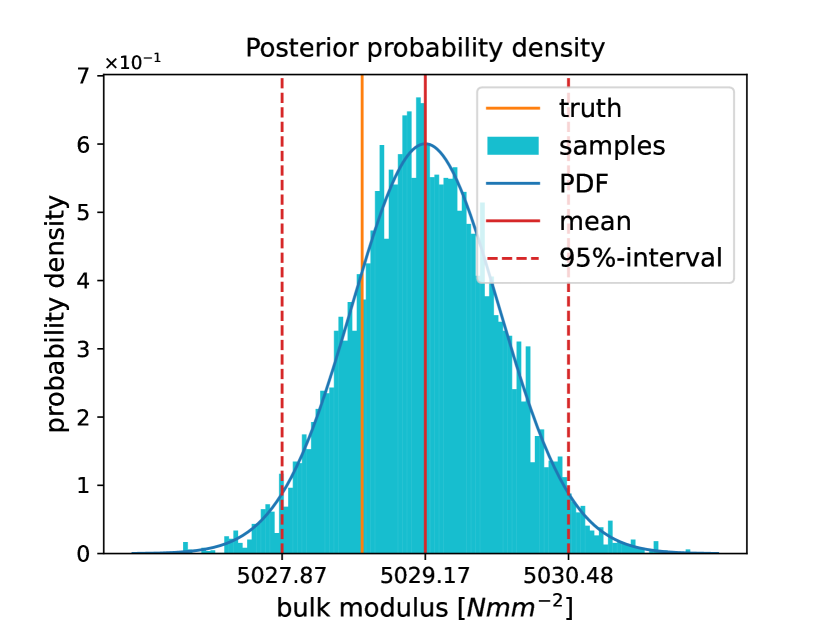
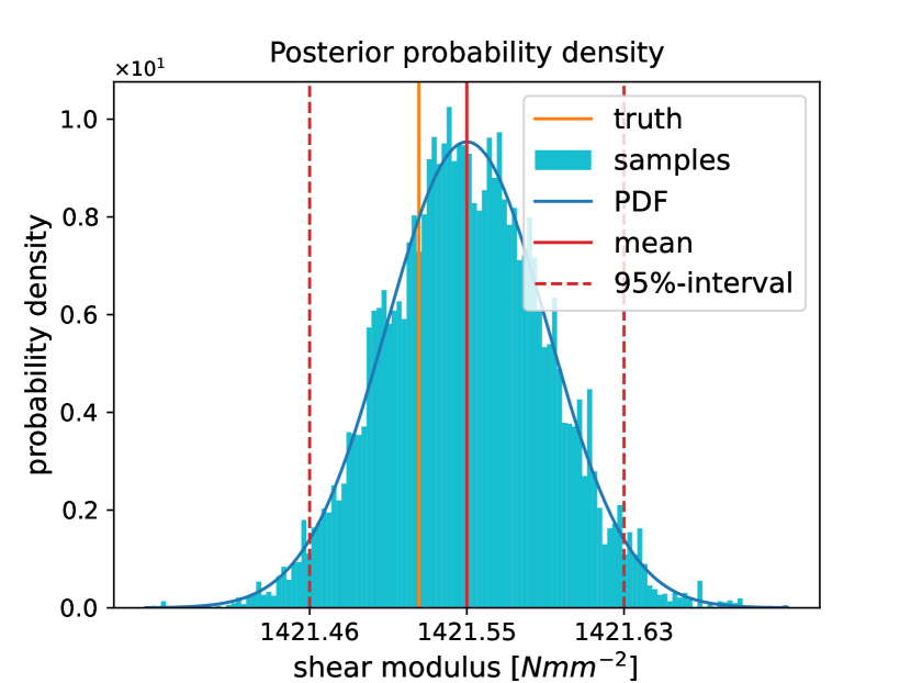
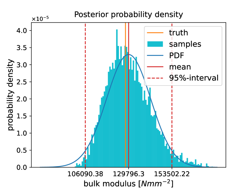
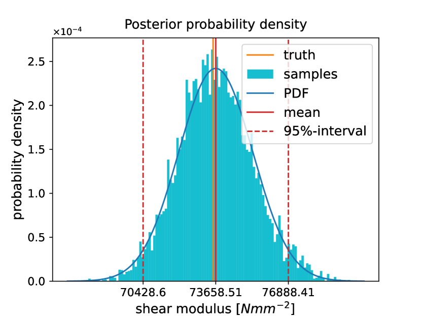
The results of the Bayesian statistical inference are listed in Table 2. The coverage test clearly shows that the estimated uncertainty is valid in the sense of frequentist statistics. For both test cases 1 and 2, the coverage for both material parameters is close to the expected . We further report the average bias of the posterior mean values with respect to the true material parameters and the standard deviations of the posterior distributions. To calculate these quantities, we have made the assumption that the sampled posterior probability density function (PDF) can be approximated by a Gaussian distribution. As shown in Fig. 3 as an example, this is a reasonable assumption. Furthermore, the runtime for the MCMC analysis is less than seconds on average on a NVIDIA GPU A100 with 80 GB memory. According to the hyperparameters of the emcee algorithm specified above, the parametric PINN is evaluated a total of times in each MCMC analysis.
| coverage |
average bias
of mean |
standard deviation | ||
|---|---|---|---|---|
| test case 1: linear elasticity | bulk modulus | |||
| shear modulus | ||||
| test case 2: hyperelasticity | bulk modulus | |||
| shear modulus |
6 Results for experimental full-field data
Finally, we showcase the calibration of the linear elastic material model from real-world experimental full-field displacement data. As with the synthetic data in Section 5, we perform both a deterministic and a statistical calibration.
6.1 Setup and training of parametric PINN
We consider experimental full-field displacement data measured in a tensile test using DIC. In the experiment, we used a specimen of S235 steel and assume linear elastic material behaviour.
Experimental settings: The specimen was clamped on the left side and the testing machine pulled on the right side in axial direction up to an averaged axial strain of . Thus, the strain is still in the linear elastic regime of the material under consideration. After a maximum traction of has been applied, the displacements in the parallel area around the hole were measured with a DIC system. For an illustration of the specimen geometry, the boundary conditions and the measurement area, please refer to Fig. 4. The full-field DIC measurement is published in [31].
FE simulations: To enhance the training process and to validate the parametric PINN, we generate high fidelity displacement data using FEM. Therefore, the simplified geometry is meshed with triangular elements and we choose linear ansatz functions with one point integration. The displacement field is then calculated and recorded for a total of nodes. Discretization errors are neglected due to the high resolution of the computational grid.
PINN’s architecture and training: The hyperparameters of the parametric PINN and the training settings are identical to the two previous test cases. To reduce the complexity, we train the parametric PINN not for the complete specimen geometry but for a simplified one, see Fig. 4. For this purpose, we transfer the stress boundary condition from the end of the clamped area where the traction was actually applied to the end of the parallel area. As a prerequisite, we make the assumption that the force is distributed homogeneously over the height of the sample.
The training data is composed as follows: We train the parametric PINN for bulk and shear moduli in the range and corresponding to ranges for Young’s modulus and Poisson’s ratio of and , respectively. For training, we consider different combinations of the material parameters drawn by Sobol sampling. For each of the parameter samples, we generate collocation points within the domain () and collocation points on each of the six boundary segments (). In addition, we enhance the training data set by pre-simulated FE data (). We randomly select data points from the FEM solution each for material parameter combinations drawn by Sobol sampling. We further weight the data loss term by in order to account for the different loss term scales.
Validation: As in the previous test cases, validation is performed on data points directly and randomly taken from the FEM solution each for randomly sampled parameter combinations within the training ranges. In relation to the validation data, the parametric PINN yields a MAE and a of and , respectively.
6.2 Deterministic calibration
The full-field displacement measurement comprises a total of data points within the parallel area around the hole, see Fig. 4 for the specimen geometry. For calibration, we again use the L-BFGS algorithm and initialize the material parameters with the mean value of their training range, respectively. As reference solution, we use the result of a NLS-FEM calibration. In this approach, the parameters-to-state map is realized by a FE simulation that is performed in each iteration instead of using the parametric PINN. For solving the NLS-FEM problem, the lsqnonlin function in Matlab is used. For more information on this approach when using full-field displacement data, please refer to [16].
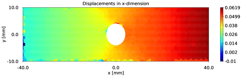
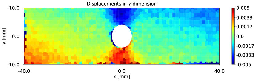
For the visualization of the DIC images in Fig. 5, the measured displacements are interpolated onto a regular grid. The visualization shows that particularly in the area around the hole and the clamping, displacements were measured that deviate significantly from the expected displacement field. Since the outliers also significantly distort the scale of the displacements in -direction, we therefore limit the scale of the displacements in -direction to for visualization purposes only. In addition, it becomes clear that the measured displacements in -direction are superimposed by a lateral displacement which may result from an eccentric clamping of the test specimen. However, it should be noted that the expected magnitude of the displacements in -direction is small compared to the -direction due to the material properties and the experimental setup. The measurement in -direction is therefore more susceptible to external disturbances.
The results of the NLS calibration are listed in Table 3. The calibration using the raw DIC data yields a bulk and shear modulus of and , respectively. In relation to the NLS-FEM results, the identified material parameters deviate by relative deviations of and . We assume that the reason for the large deviation is that the displacement data is pre-processed in NLS-FEM. The measured full-field displacement data is linearly interpolated onto the FE mesh nodes. In this process, outliers in the full-field measurement are smoothed out. For the linear interpolation, the Matlab function scatteredInterpolant with default settings is used. The parametric PINN, on the other hand, uses the raw measurement data without pre-processing. For a fair comparison, we therefore also carry out the calibration with the interpolated displacement measurements. After interpolation, the full-field displacement measurement comprises a total of data points. The calibration using the interpolated data results in a bulk and shear modulus of and , respectively, which deviate by RDs of and from the NLS-FEM results. Furthermore, with the parametric PINN, the runtime for the NLS calibration is less than five seconds on a NVIDIA GPU A100 with 80 GB memory. Both the parametric PINN and the FE model are evaluated times.
| bulk modulus | shear modulus | |
|---|---|---|
| FEM (interpolated data) | ||
| PINN (raw data) | ||
| PINN (interpolated data) | ||
6.3 Statistical calibration
Finally, we determine the posterior distribution of the material parameters in the linear elastic constitutive model for the real-world experimental full-field displacement data. A detailed description of the experimental setup is given in Section 6.1. In order to validate our results for the parametric PINN, we compare the posterior distributions to the results with FEM as parameters-to-state map. As we found out in Section 6.2, for a fair comparison, we need to use the interpolated displacement data. Furthermore, for the MCMC analysis, we employ the emcee algorithm with an ensemble of workers each with a chain length of and a stretch scale of . Samples are recorded after a burn-in phase with a chain length of for each worker. The workers are initialized randomly within the material parameter training ranges.
In the first attempt, we assumed Gaussian noise with zero mean and standard deviation just like with the synthetic data. However, without further modifications, we have not obtained reasonable results for this noise level. We suspect two possible reasons for the failure of the MCMC analysis:
-
(i)
First, the noise in the present data is superimposed by measurement artifacts, such as lateral displacements due to a possibly eccentric clamping of the specimen. Additionally, in Fig. 5, we can see some measurement outliers close to the boundary caused by errors in the facet-matching in consequence of a slightly incorrect placement of the tensile specimen with respect to the camera alignment. The resulting measurement error which is made up of the background noise and the measurement artifacts is therefore probably greater than the assumed value of .
-
(ii)
Second, we assume that the noise levels for the present data are actually different in the - and - directions. One possible reason for this is the different resolution of the DIC system in the different spatial directions. In addition, in the deterministic setting, we have already observed that weighting the residuals is essential for the calibration from experimental data.
We therefore propose to use the diagonal covariance matrix obtained from relating the NLS problem to the maximum a posteriori estimate, see 41–42. If we use a uniform prior over the admissible set of material parameters , we restrict the statistical calibration problem to the same parameter set as the deterministic NLS problem, see 36. With a uniform prior, the logarithm of the prior in 42 is constant and can be neglected in the minimization problem. The maximum a posteriori estimate then simplifies to the so-called maximum likelihood estimate
| (43) | ||||
For uniform priors, the diagonal covariance matrix can then be related to the weight matrix in the NLS problem 35 by
| (44) |
where the sub-covariance matrices for i.i.d. noise are defined as
| (45) |
with the identity matrix of size and standard deviations and of Gaussian noise and in - and -direction, respectively.
In the following, we use a uniform prior for the material parameters to be inferred and derive the covariance matrix from 43, 44 and 45 as described above. For the weight matrix used in the NLS problem, we finally obtain standard deviations and for i.i.d. Gaussian noise and in - and -direction, respectively.
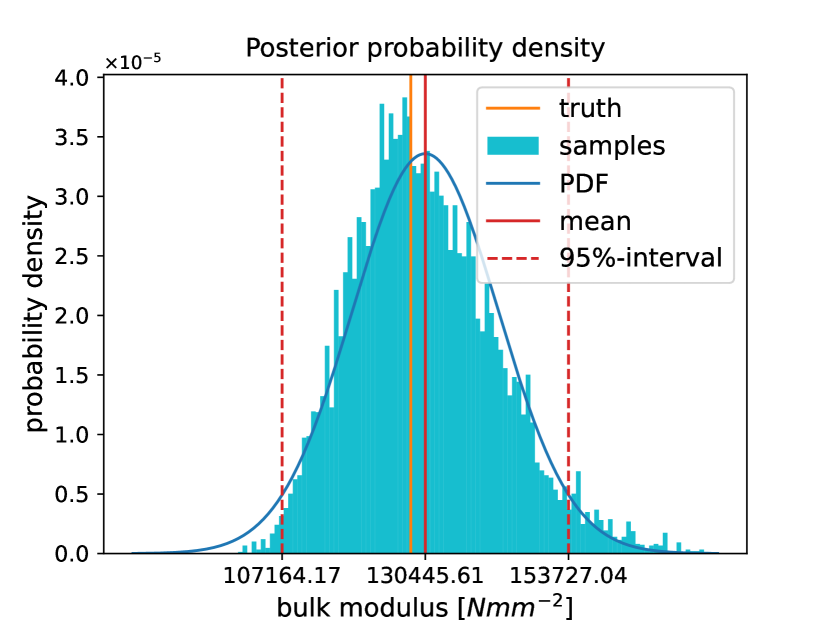
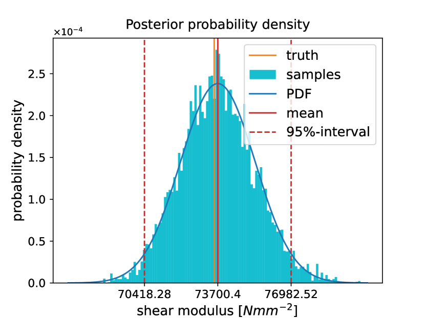
The posterior probability densities for bulk and shear modulus obtained by a MCMC analysis are illustrated in Fig. 7(a). The probability distributions show a good concentration and small uncertainties for both material parameters. Furthermore, the mean values of the posterior probability densities are close to the values we obtain from the deterministic NLS-FEM calibration. This is expected since we derive the covariance matrix from the relation between the maximum a posteriori estimate and the NLS problem. For validation, we also carry out the MCMC analysis with FEM as parameters-to-state map and the same covariance matrix, see Fig. 7(b). The comparison shows that the posterior probability densities obtained with the two different methods are in good agreement. Moreover, with the parametric PINN, the runtime for the MCMC analysis is less than seconds on a NVIDIA GPU A100 with 80 GB memory. According to the hyperparameters of the emcee algorithm specified above, the parametric PINN is evaluated a total of times in the MCMC analysis.
Finally, we would like to make the following remarks: First, PINNs generally do not well extrapolate beyond the training domain. We therefore recommend the use of material parameter priors with at most weak support beyond the training range of the parametric PINN. Otherwise, the Markov chain is more likely to explore regions in the parameter domain for which the parametric PINN is not trained and thus does not provide good prediction accuracy. As mentioned before, in Bayesian inference, a correct uncertainty quantification relies on a accurate parameters-to-state map. Second, it should be noted that the noise levels derived from the weights used in the corresponding NLS problem are not the actual noise levels of the measurements. The choice of the weights is usually based on heuristics and not necessarily on a statistical analysis of the measurement data. However, the chosen approach enables comparability between the statistical and the deterministic calibration problems. Third, we point out that Bayesian inference, in principle, also allows the noise level to be estimated simultaneously with the material parameters. Therefore, the noise can be modeled, e.g., by Gaussian distributions or by Gaussian processes [62]. However, estimating the noise is beyond the scope of this work. For more information on this approach, we refer, for instance, to [63].
7 Conclusion and outlook
Advances in the development of full-field measurement capabilities, such as, e.g., digital image correlation (DIC), have recently led to an increasing interest in appropriate methods for the calibration of constitutive models. In experimental mechanics, the inverse problem of identifying the material parameters is traditionally solved by numerical methods, such as nonlinear least-squares finite element method (NLS-FEM) or virtual fields method (VFM). However, the computational costs associated with these methods are oftentimes to high, making them unsuitable for online applications. This results in an urgent need for methods that enable rapid calibration in online applications, even under severe time constraints.
In the present contribution, we demonstrate that the parametric PINN approach enables an accurate and efficient model calibration and uncertainty quantification of the inferred material parameters. In the offline stage, the parametric PINN is trained to learn a parameterized solution of the underlying parametric partial differential equation (PDE) by encoding the physics into a loss function. In addition, training can be enhanced by high-fidelity simulation data that can be easily integrated into the training process. In the subsequent online stage, the parametric PINN then can be employed as a surrogate for the parameters-to-state map in the calibration process. Due to the low computational costs of artificial neural network (ANN) evaluations, calibration can be performed in near real-time, even though ten thousands of forward model evaluations are required.
We demonstrated the advantages of using parametric PINNs for constitutive model calibration in deterministic nonlinear least-squares (NLS) calibration as well as Markov chain Monte Carlo (MCMC)-based Bayesian inference in various numerical tests. First, we considered the calibration of a small strain linear elastic and a finite strain hyperelastic constitutive model using noisy synthetic data. A statistical evaluation of the results showed both high accuracy for the deterministic point estimate and valid uncertainty for the Bayesian inference. In addition, we calibrated a small strain linear elastic model using experimental full-field data from a tensile test. As reference, we used the results obtained when using the finite element method (FEM) instead of the parametric PINN as parameters-to-state map. The parametric PINN also showed good results for the experimental data in both the deterministic and statistical settings. At the same time, the runtime of the parametric PINN needed for online calibration is considerably shorter, especially when it comes to MCMC-based Bayesian inference.
To the best of the authors knowledge, this is the first contribution which presents parametric PINNs for the calibration of constitutive models. While it has often been stated that PINNs are especially suited for inverse problems, the settings considered in the literature so far are often far away from realistic applications. Herein, the authors have demonstrated the entire process from parametric PINN training towards model calibration using real-world experimental data. The achieved savings in the online calibration step urge for further developments of parametric PINNs for more complex, history dependent and anisotropic materials. The pre-training of parametric PINNs may help to further establish full-field measurement techniques, such as DIC, in materials development in both academia and industry as well as in online applications, such as continuous structural health monitoring (SHM).
Although the parametric PINNs have already achieved good results in our numerical tests, further work is necessary for real-world applications. In the example with the experimental data, it became clear that the real measurement data can also contain measurement artifacts in addition to the background noise of the DIC system. In contrast to the background noise, the measurement artifacts are difficult to characterize and make calibration more challenging. This applies in particular to PINNs as they usually use the data directly, without prior interpolation of the sensor data. For this reason, either a pre-processing of the data is necessary before calibration, or the additional uncertainties must be taken into account during calibration. Possible methods for pre-processing are, among others, polynomial interpolation [64], ANN-based interpolation [65] or kernel methods [66]. In a statistical setting, the measurement error could also be considered as an additional error term in 39a and modeled, e.g., by a Gaussian process [63].
The authors are aware that a reliable measurement of full-field displacement data using, e.g., a DIC system, places very high demands on the measurement system. These requirements are significantly higher for on-site online applications in SHM compared to laboratory applications due to the environmental impacts acting on the system. However, the use of DIC in the context of SHM is an active field of research, see, e.g., [67, 68, 69].
From a modeling perspective, a further challenge arises as soon as the displacement or load boundary conditions are not constant. This is particularly likely for applications in the field of SHM. The load boundary condition then needs to be inferred online using, e.g., load cells [70]. However, every boundary condition that is not exactly known before training must be taken into account as a parameter and thus as an additional input to the parametric PINN. This means that future work on methods for overcoming the curse of dimensionality are also of great importance.
Declarations
Availability of data and materials
Competing interests
The authors declare that they have no competing interests.
Funding
DA, HW and UR acknowledge support by the Deutsche Forschungsgemeinschaft (DFG, German Research Foundation) in the project DFG 255042459: ”GRK2075: Modeling the constitutional evolution of building materials and structures with respect to aging”. DA and HW also acknowledge support in the project DFG 501798687: ”Monitoring data driven life cycle management with AR based on adaptive, AI-supported corrosion prediction for reinforced concrete structures under combined impacts” which is a subproject of SPP 2388: ”Hundred plus - Extending the Lifetime of Complex Engineering Structures through Intelligent Digitalization” funded by the DFG. AH acknowledges support by an ETH Zurich Postdoctoral Fellowship.
Authors’ contributions
DA: conceptualization, data curation, formal analysis, investigation, methodology, project administration, software, validation, visualization, writing – original draft, writing – review and editing; JAT: data curation, investigation, software, validation, writing – original draft, writing – review and editing; HW: conceptualization, funding acquisition, methodology, resources, supervision, writing – original draft, writing – review and editing; UR: conceptualization, funding acquisition, methodology, supervision, writing – review and editing; AH: conceptualization, supervision, writing – review and editing; SH: resources, supervision, writing – review and editing.
Acknowledgements
DA, HW and UR thank the members of the research training group GRK2075 for the fruitful discussions.
Appendix A Boundary conditions in strong form PINNs
We consider the balance equation 2 with boundary conditions 3 for the top left quadrant of a plate with a hole as described in Section 5.1. The same test case has been considered earlier in [71], where it has been reported that the accuracy of strong form PINNs was insufficient. Herein, we illustrate that the reason for the unsatisfactory results is merely an incomplete imposition of BCs in [71]. Note that in Galerkin Finite Element Methods, Neumann BCs are treated via surface integrals, and zero traction BCs are automatically fulfilled. This is not the case for methods relying on the strong form.
To this end, we exemplary consider the right boundary of the plate sketched in Fig. 8, where the following BCs must be fulfilled:
| (46a) | ||||
| (46b) | ||||
In [71], only the Dirichlet condition 46a has been considered, see also Fig. 8(a). However, since the balance of linear momentum 2 results in two coupled PDEs for the considered 2D test case, at each boundary two BCs need to be defined, one in each spatial dimension. With the surface normal of the right boundary , the Neumann BC 46b follows directly from :
| (47) | ||||
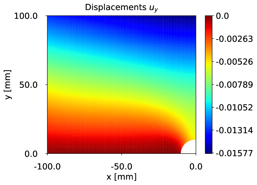
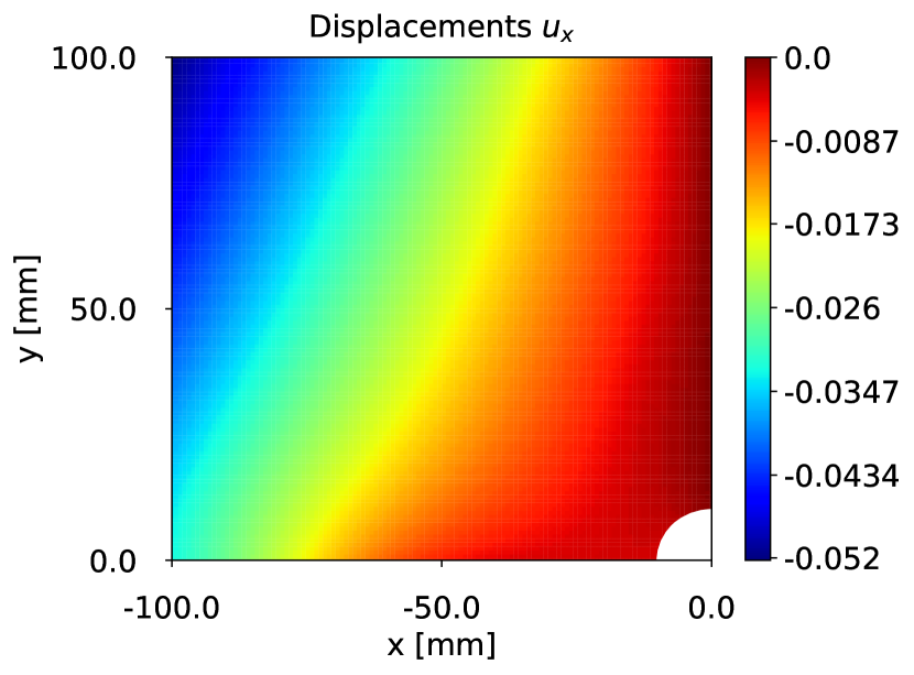
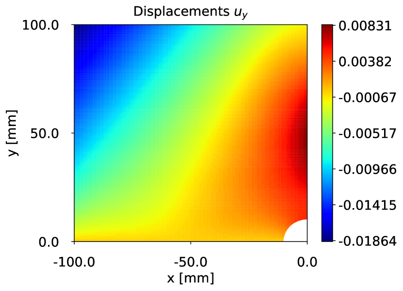
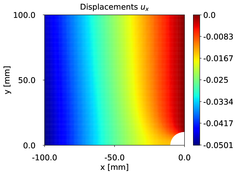
To illustrate that the correct application of BCs is essential, we solve the forward problem for the top left quadrant of a plate with a hole with and without symmetry stress BCs and compare the results. The geometry and BCs are shown in Fig. 8. We use the ansatz 23 with a fully connected feed-forward neural network (FFNN) with six hidden layers each with neurons and hyperbolic tangent activation functions. The weights and biases of the FFNN are initialized according to Glorot normal initialization [58] and with zeros, respectively. The training data set consists of collocation points within the domain and points on each of the five boundary segments. No FE data is used for training. We train the PINN for a predefined bulk modulus and shear modulus , respectively. The resulting optimization problem is solved using the L-BFGS optimization algorithm [46, 47, 48, 49, 50].
The mean absolute error (MAE) and the relative norm () of the PINN solution with and without symmetry stress BCs compared to a high-fidelity FE solution are summarized in Table 4. For validation, we randomly select points from the FE solution. In addition, we show the PINN solutions we obtained with and without symmetry stress BCs as well as the FE reference solution in Fig. 9.
| with symmetry stress BCs | without symmetry stress BCs | |
|---|---|---|
| MAE | ||


Appendix B Error measures
In order to validate the performance of our parametric PINN formulation, we compare the PINN predictions to the solutions of high-fidelity finite element (FE) simulations. We consider the MAE as an absolute error measure and the as a relative error measure. In the following, represents the vector containing the displacements of all nodes with coordinates in the FE discretization. The vector contains the displacements predicted by the parametric PINN where the PINN is evaluated according to 29 at the coordinates . The same material parameters are used for both the FE simulation and the evaluation of the parametric PINN.
For the statistical evaluation of the calibration results, we consider the absolute relative error (ARE). In addition to the mean, minimum and maximum ARE, we also calculate the standard error of the mean (SEM) which gives us information about the scatter of the ARE. Here, represents the vector of true material parameters and the vector of material parameters identified by using the parametric PINN as parameters-to-state map in the deterministic least-squares calibration.
The absolute relative error (ARE) for material parameter is defined as
| (50) |
The standard error of the mean (SEM) with respect to a certain error measure, for instance, the ARE, is then calculated as
| (51) |
where is the number of test cases on which the statistical evaluation is based and is the standard deviation, e.g., of the ARE.
References
- \bibcommenthead
- Chang [1998] Chang, F.-K.: Structural Health Monitoring: A Summary Report on the First Stanford Workshop on Structural Health Monitoring, September 18-20, 1997. Technical report, Stanford University (1998). https://doi.org/10.21236/ADA350933
- Entezami [2021] Entezami, A.: Structural Health Monitoring by Time Series Analysis and Statistical Distance Measures, 1st edn. SpringerBriefs in Applied Sciences and Technology. Springer, Cham (2021). https://doi.org/10.1007/978-3-030-66259-2
- Sutton et al. [2009] Sutton, M.A., Orteu, J.-J., Schreier, H.: Image Correlation for Shape, Motion and Deformation Measurements, 1st edn. Springer, New York (2009). https://doi.org/10.1007/978-0-387-78747-3
- Yang and Ettemeyer [2003] Yang, L.X., Ettemeyer, A.: Strain measurement by three-dimensional electronic speckle pattern interferometry: potentials, limitations, and applications. Optical Engineering 42(5), 1257–1266 (2003) https://doi.org/10.1117/1.1566781
- Mahnken and Stein [1996] Mahnken, R., Stein, E.: A unified approach for parameter identification of inelastic material models in the frame of the finite element method. Computer Methods in Applied Mechanics and Engineering 136(3), 225–258 (1996) https://doi.org/10.1016/0045-7825(96)00991-7
- Rose and Menzel [2020] Rose, L., Menzel, A.: Optimisation based material parameter identification using full field displacement and temperature measurements. Mechanics of Materials 145, 103292 (2020) https://doi.org/%****␣main.bbl␣Line␣125␣****10.1016/j.mechmat.2019.103292
- Avril et al. [2008] Avril, S., Bonnet, M., Bretelle, A.-S., Grédiac, M., Hild, F., Ienny, P., Latourte, F., Lemosse, D., Pagano, S., Pagnacco, E., Pierron, F.: Overview of Identification Methods of Mechanical Parameters Based on Full-field Measurements. Experimental Mechanics 48(4), 381–402 (2008) https://doi.org/10.1007/s11340-008-9148-y
- Martins et al. [2018] Martins, J.M.P., Andrade-Campos, A., Thuillier, S.: Comparison of inverse identification strategies for constitutive mechanical models using full-field measurements. International Journal of Mechanical Sciences 145, 330–345 (2018) https://doi.org/10.1016/j.ijmecsci.2018.07.013
- Raissi et al. [2019] Raissi, M., Perdikaris, P., Karniadakis, G.E.: Physics-informed neural networks: A deep learning framework for solving forward and inverse problems involving nonlinear partial differential equations. Journal of Computational Physics 378, 686–707 (2019) https://doi.org/10.1016/j.jcp.2018.10.045
- Karniadakis et al. [2021] Karniadakis, G.E., Kevrekidis, I.G., Lu, L., Perdikaris, P., Wang, S., Yang, L.: Physics-informed machine learning. Nature Reviews Physics 3(6), 422–440 (2021) https://doi.org/10.1038/s42254-021-00314-5
- Psichogios and Ungar [1992] Psichogios, D.C., Ungar, L.H.: A hybrid neural network-first principles approach to process modeling. American Institute of Chemical Engineers Journal 38(10), 1499–1511 (1992) https://doi.org/10.1002/aic.690381003
- Lagaris et al. [1998] Lagaris, I.E., Likas, A., Fotiadis, D.I.: Artificial neural networks for solving ordinary and partial differential equations. IEEE Transactions on Neural Networks 9(5), 987–1000 (1998) https://doi.org/%****␣main.bbl␣Line␣225␣****10.1109/72.712178
- Baydin et al. [2018] Baydin, A.G., Pearlmutter, B.A., Radul, A.A., Siskind, J.M.: Automatic differentiation in machine learning: a survey. Journal of Machine Learning Research 18(1), 5595–5637 (2018)
- Abadi et al. [2015] Abadi, M., Agarwal, A., Barham, P., Brevdo, E., Chen, Z., Citro, C., Corrado, G.S., Davis, A., Dean, J., Devin, M., Ghemawat, S., Goodfellow, I., Harp, A., Irving, G., Isard, M., Jia, Y., Jozefowicz, R., Kaiser, L., Kudlur, M., Levenberg, J., Mané, D., Monga, R., Moore, S., Murray, D., Olah, C., Schuster, M., Shlens, J., Steiner, B., Sutskever, I., Talwar, K., Tucker, P., Vanhoucke, V., Vasudevan, V., Viégas, F., Vinyals, O., Warden, P., Wattenberg, M., Wicke, M., Yu, Y., Zheng, X.: TensorFlow: Large-Scale Machine Learning on Heterogeneous Systems. Software available from tensorflow.org (2015). https://www.tensorflow.org/
- Paszke et al. [2019] Paszke, A., Gross, S., Massa, F., Lerer, A., Bradbury, J., Chanan, G., Killeen, T., Lin, Z., Gimelshein, N., Antiga, L., Desmaison, A., Köpf, A., Yang, E., DeVito, Z., Raison, M., Tejani, A., Chilamkurthy, S., Steiner, B., Fang, L., Bai, J., Chintala, S.: PyTorch: An imperative style, high-performance deep learning library. arXiv Preprint (2019) https://doi.org/10.48550/arXiv.1912.01703 . Software available from pytorch.org
- Römer et al. [2024] Römer, U., Hartmann, S., Tröger, J.-A., Anton, D., Wessels, H., Flaschel, M., De Lorenzis, L.: Reduced and all-at-once approaches for model calibration and discovery in computational solid mechanics. arXiv Preprint (2024) https://doi.org/10.48550/arXiv.2404.16980
- Shukla et al. [2022] Shukla, K., Jagtap, A.D., Blackshire, J.L., Sparkman, D., Karniadakis, G.E.: A Physics-Informed Neural Network for Quantifying the Microstructural Properties of Polycrystalline Nickel Using Ultrasound Data: A Promising Approach for Solving Inverse Problems. IEEE Signal Processing Magazine 39(1), 68–77 (2022) https://doi.org/10.1109/MSP.2021.3118904
- Rojas et al. [2023] Rojas, C.J.G., Boldrini, J.L., Bittencourt, M.L.: Parameter identification for a damage phase field model using a physics-informed neural network. Theoretical and Applied Mechanics Letters 13(3), 100450 (2023) https://doi.org/10.1016/j.taml.2023.100450
- Zhang et al. [2022] Zhang, E., Dao, M., Karniadakis, G.E., Suresh, S.: Analyses of internal structures and defects in materials using physics-informed neural networks. Science Advances 8(7), 0644 (2022) https://doi.org/10.1126/sciadv.abk0644
- Haghighat et al. [2021] Haghighat, E., Raissi, M., Moure, A., Gomez, H., Juanes, R.: A physics-informed deep learning framework for inversion and surrogate modeling in solid mechanics. Computer Methods in Applied Mechanics and Engineering 379, 113741 (2021) https://doi.org/10.1016/j.cma.2021.113741
- Hamel et al. [2022] Hamel, C.M., Long, K.N., Kramer, S.L.B.: Calibrating constitutive models with full-field data via physics informed neural networks. Strain 59(2), 12431 (2022) https://doi.org/10.1111/str.12431
- Zhang et al. [2020] Zhang, E., Yin, M., Karniadakis, G.E.: Physics-informed neural networks for nonhomogeneous material identification in elasticity imaging. arXiv Preprint (2020) https://doi.org/10.48550/arXiv.2009.04525
- Anton and Wessels [2023] Anton, D., Wessels, H.: Physics-informed neural networks for material model calibration from full-field displacement data. arXiv Preprint (2023) https://doi.org/10.48550/arXiv.2212.07723
- Hosseini et al. [2023] Hosseini, E., Scheel, P., Müller, O., Molinaro, R., Mishra, S.: Single-track thermal analysis of laser powder bed fusion process: Parametric solution through physics-informed neural networks. Computer Methods in Applied Mechanics and Engineering 410, 116019 (2023) https://doi.org/10.1016/j.cma.2023.116019
- Beltrán-Pulido et al. [2022] Beltrán-Pulido, A., Bilionis, I., Aliprantis, D.: Physics-Informed Neural Networks for Solving Parametric Magnetostatic Problems. IEEE Transactions on Energy Conversion 37(4), 2678–2689 (2022) https://doi.org/10.1109/TEC.2022.3180295
- Sun et al. [2023] Sun, Y., Sengupta, U., Juniper, M.: Physics-informed deep learning for simultaneous surrogate modeling and PDE-constrained optimization of an airfoil geometry. Computer Methods in Applied Mechanics and Engineering 411, 116042 (2023) https://doi.org/10.1016/j.cma.2023.116042
- Agarwal et al. [2024] Agarwal, G., Urrea-Quintero, J.-H., Wessels, H., Wick, T.: Model order reduction for transient coupled diffusion-deformation of hydrogels. arXiv Preprint (2024) https://doi.org/10.48550/arXiv.2403.08968
- Stoter et al. [2022] Stoter, S.K.F., Jessen, E., Niedens, V., Schillinger, D.: A DEIM driven reduced basis method for the diffuse Stokes/Darcy model coupled at parametric phase-field interfaces. Computational Geosciences 26(6), 1465–1502 (2022) https://doi.org/10.1007/s10596-022-10164-4
- Baratta et al. [2023] Baratta, I.A., Dean, J.P., Dokken, J.S., Habera, M., Hale, J.S., Richardson, C.N., Rognes, M.E., Scroggs, M.W., Sime, N., Wells, G.N.: DOLFINx: The next generation FEniCS problem solving environment. Zenodo. Software available from github.com/FEniCS/dolfinx (2023). https://doi.org/10.5281/zenodo.10447666
- Anton [2024] Anton, D.: Code for the publication ”Deterministic and statistical calibration of constitutive models from full-field data with parametric physics-informed neural networks”. Zenodo. Code available from https://github.com/david-anton/CalibrationPINN (2024). https://doi.org/10.5281/zenodo.11368998
- Tröger et al. [2024] Tröger, J.-A., Hartmann, S., Anton, D., Wessels, H.: Digital image correlation measurement of linear elastic steel specimen. Zenodo. Data set (2024). https://doi.org/10.5281/zenodo.11257192
- Holzapfel [2000] Holzapfel, G.A.: Nonlinear Solid Mechanics: A Continuum Approach for Engineering, 1st edn. Wiley, Chichester (2000)
- Wriggers [2008] Wriggers, P.: Nonlinear Finite Element Methods, 1st edn. Springer, Berlin (2008). https://doi.org/10.1007/978-3-540-71001-1
- Marsden and Hughes [1983] Marsden, J., Hughes, T.J.R.: Mathematical Foundations of Elasticity, 1st edn. Dover Books on Mathematics. Dover Publications, New York (1983)
- Lychev and Koifman [2019] Lychev, S., Koifman, K.: Geometry of Incompatible Deformations: Differential Geometry in Continuum Mechanics. De Gruyter Studies in Mathematical Physics. De Gruyter, Berlin (2019). https://doi.org/10.1515/9783110563214
- Ehlers and Eipper [1998] Ehlers, W., Eipper, G.: The simple tension problem at large volumetric strains computed from finite hyperelastic material laws. Acta Mechanica 130(1), 17–27 (1998) https://doi.org/10.1007/BF01187040
- Hartmann and Neff [2003] Hartmann, S., Neff, P.: Polyconvexity of generalized polynomial-type hyperelastic strain energy functions for near-incompressibility. International Journal of Solids and Structures 40(11), 2767–2791 (2003) https://doi.org/%****␣main.bbl␣Line␣650␣****10.1016/S0020-7683(03)00086-6
- Goodfellow et al. [2016] Goodfellow, I., Bengio, Y., Courville, A.: Deep Learning. MIT Press, online (2016). https://www.deeplearningbook.org
- Cybenko [1989] Cybenko, G.: Approximation by superpositions of a sigmoidal function. Mathematics of Control, Signals, and Systems 2(4), 303–314 (1989) https://doi.org/10.1007/BF02551274
- Hornik et al. [1989] Hornik, K., Stinchcombe, M., White, H.: Multilayer feedforward networks are universal approximators. Neural Networks 2(5), 359–366 (1989) https://doi.org/10.1016/0893-6080(89)90020-8
- Li [1996] Li, X.: Simultaneous approximations of multivariate functions and their derivatives by neural networks with one hidden layer. Neurocomputing 12(4), 327–343 (1996) https://doi.org/10.1016/0925-2312(95)00070-4
- Berg and Nyström [2018] Berg, J., Nyström, K.: A unified deep artificial neural network approach to partial differential equations in complex geometries. Neurocomputing 317, 28–41 (2018) https://doi.org/10.1016/j.neucom.2018.06.056
- LeCun et al. [2012] LeCun, Y.A., Bottou, L., Orr, G.B., Müller, K.-R.: Efficient BackProp. In: Montavon, G., Orr, G.B., Müller, K.-R. (eds.) Neural Networks: Tricks of the Trade, 2nd edn. Lecture Notes in Computer Science, pp. 9–48. Springer, Berlin (2012). https://doi.org/10.1007/978-3-642-35289-8_3
- Wang et al. [2021] Wang, S., Teng, Y., Perdikaris, P.: Understanding and Mitigating Gradient Flow Pathologies in Physics-Informed Neural Networks. SIAM Journal on Scientific Computing 43(5), 3055–3081 (2021) https://doi.org/10.1137/20M1318043
- Kingma and Ba [2015] Kingma, D.P., Ba, J.L.: Adam: A Method for Stochastic Optimization. In: Bengio, Y., LeCun, Y. (eds.) 3rd International Conference on Learning Representations, ICLR 2015, San Diego, CA, USA, May 7-9, 2015, Conference Track Proceedings (2015)
- Liu and Nocedal [1989] Liu, D.C., Nocedal, J.: On the limited memory BFGS method for large scale optimization. Mathematical Programming 45(1), 503–528 (1989) https://doi.org/10.1007/BF01589116
- Broyden [1970] Broyden, C.G.: The Convergence of a Class of Double-rank Minimization Algorithms 1. General Considerations. IMA Journal of Applied Mathematics 6(1), 76–90 (1970) https://doi.org/10.1093/imamat/6.1.76
- Fletcher [1970] Fletcher, R.: A new approach to variable metric algorithms. The Computer Journal 13(3), 317–322 (1970) https://doi.org/10.1093/comjnl/13.3.317
- Goldfarb [1970] Goldfarb, D.: A family of variable-metric methods derived by variational means. Mathematics of Computation 24(109), 23–26 (1970) https://doi.org/10.2307/2004873
- Shanno [1970] Shanno, D.F.: Conditioning of quasi-Newton methods for function minimization. Mathematics of Computation 24(111), 647–656 (1970) https://doi.org/10.2307/2004840
- Krantz and Parks [2013] Krantz, S.G., Parks, H.R.: The Implicit Function Theorem: History, Theory, and Applications, 1st edn. Modern Birkhäuser Classics. Birkhäuser, New York (2013). https://doi.org/%****␣main.bbl␣Line␣850␣****10.1007/978-1-4614-5981-1
- Lawson and Hanson [1995] Lawson, C.L., Hanson, R.J.: Solving Least Squares Problems, 1st edn. Classics in Applied Mathematics. Society for Industrial and Applied Mathematics, Philadelphia (1995). https://doi.org/10.1137/1.9781611971217
- Mahnken [2017] Mahnken, R.: Identification of Material Parameters for Constitutive Equations, 2nd edn., pp. 1–21. Wiley, Hoboken (2017). https://doi.org/10.1002/9781119176817.ecm2043
- Gelman et al. [2013] Gelman, A., Carlin, J.B., Stern, H.S., Dunson, D.B., Vehtari, A., Rubin, D.B.: Bayesian Data Analysis, 3rd edn. Texts in Statistical Science. Chapman and Hall/CRC, New York (2013). https://doi.org/10.1201/b16018
- Goodman and Weare [2010] Goodman, J., Weare, J.: Ensemble samplers with affine invariance. Communications in Applied Mathematics and Computational Science 5(1), 65–80 (2010) https://doi.org/10.2140/camcos.2010.5.65
- Foreman-Mackey et al. [2013] Foreman-Mackey, D., Hogg, D.-W., Lang, D., Goodman, J.: emcee: The MCMC Hammer. Publications of the Astronomical Society of the Pacific 125(925), 306–312 (2013) https://doi.org/10.1086/670067
- Kleijn and van der Vaart [2012] Kleijn, B.J.K., Vaart, A.W.: The Bernstein-Von-Mises theorem under misspecification. Electronic Journal of Statistics 6(none), 354–381 (2012) https://doi.org/10.1214/12-EJS675
- Glorot and Bengio [2010] Glorot, X., Bengio, Y.: Understanding the difficulty of training deep feedforward neural networks. In: Teh, Y.W., Titterington, M. (eds.) Proceedings of the Thirteenth International Conference on Artificial Intelligence and Statistics. Proceedings of Machine Learning Research, vol. 9, pp. 249–256. PMLR, Sardinia (2010). https://proceedings.mlr.press/v9/glorot10a.html
- Sobol’ [1967] Sobol’, I.M.: On the distribution of points in a cube and the approximate evaluation of integrals. USSR Computational Mathematics and Mathematical Physics 7(4), 86–112 (1967) https://doi.org/10.1016/0041-5553(67)90144-9
- Pierron et al. [2010] Pierron, F., Avril, S., Tran, V.T.: Extension of the virtual fields method to elasto-plastic material identification with cyclic loads and kinematic hardening. International Journal of Solids and Structures 47(22), 2993–3010 (2010) https://doi.org/10.1016/j.ijsolstr.2010.06.022
- Hartmann et al. [2023] Hartmann, S., Müller-Lohse, L., Tröger, J.-A.: Temperature Gradient Determination with Thermography and Image Correlation in Curved Surfaces with Application to Additively Manufactured Components. Experimental Mechanics 63(1), 43–61 (2023) https://doi.org/10.1007/s11340-022-00886-y
- Rasmussen and Williams [2005] Rasmussen, C.E., Williams, C.K.I.: Gaussian Processes for Machine Learning, 1st edn. MIT Press, Cambridge (2005). https://doi.org/10.7551/mitpress/3206.001.0001
- Kennedy and O’Hagan [2001] Kennedy, M.C., O’Hagan, A.: Bayesian Calibration of Computer Models. Journal of the Royal Statistical Society Series B: Statistical Methodology 63(3), 425–464 (2001) https://doi.org/10.1111/1467-9868.00294
- Rudy et al. [2017] Rudy, S.H., Brunton, S.L., Proctor, J.L., Kutz, J.N.: Data-driven discovery of partial differential equations. Science Advances 3(4), 1602614 (2017) https://doi.org/10.1126/sciadv.1602614
- Berg and Nyström [2019] Berg, J., Nyström, K.: Data-driven discovery of PDEs in complex datasets. Journal of Computational Physics 384, 239–252 (2019) https://doi.org/10.1016/j.jcp.2019.01.036
- Flaschel et al. [2021] Flaschel, M., Kumar, S., De Lorenzis, L.: Unsupervised discovery of interpretable hyperelastic constitutive laws. Computer Methods in Applied Mechanics and Engineering 381, 113852 (2021) https://doi.org/10.1016/j.cma.2021.113852
- Dong and Catbas [2021] Dong, C.-Z., Catbas, F.N.: A review of computer vision–based structural health monitoring at local and global levels. Structural Health Monitoring 20(2), 692–743 (2021) https://doi.org/10.1177/1475921720935585
- Niezrecki et al. [2019] Niezrecki, C., Baqersad, J., Sabato, A.: In: Ida, N., Meyendorf, N. (eds.) Digital Image Correlation Techniques for NDE and SHM, pp. 1545–1590. Springer, Cham (2019). https://doi.org/10.1007/978-3-319-26553-7_47
- Reagan et al. [2018] Reagan, D., Sabato, A., Niezrecki, C.: Feasibility of using digital image correlation for unmanned aerial vehicle structural health monitoring of bridges. Structural Health Monitoring 17(5), 1056–1072 (2018) https://doi.org/10.1177/1475921717735326
- Moreno-Gomez et al. [2018] Moreno-Gomez, A., Perez-Ramirez, C.A., Dominguez-Gonzalez, A., Valtierra-Rodriguez, M., Chavez-Alegria, O., Amezquita-Sanchez, J.P.: Sensors Used in Structural Health Monitoring. Archives of Computational Methods in Engineering 25(4), 901–918 (2018) https://doi.org/10.1007/s11831-017-9217-4
- Li et al. [2021] Li, W., Bazant, M.Z., Zhu, J.: A physics-guided neural network framework for elastic plates: Comparison of governing equations-based and energy-based approaches. Computer Methods in Applied Mechanics and Engineering 383, 113933 (2021) https://doi.org/10.1016/j.cma.2021.113933
- Henkes et al. [2022] Henkes, A., Wessels, H., Mahnken, R.: Physics informed neural networks for continuum micromechanics. Computer Methods in Applied Mechanics and Engineering 393, 114790 (2022) https://doi.org/10.1016/j.cma.2022.114790