Learning Staged Trees from Incomplete Data

Abstract

Staged trees are probabilistic graphical models capable of representing any class of non-symmetric independence via a coloring of its vertices. Several structural learning routines have been defined and implemented to learn staged trees from data, under the frequentist or Bayesian paradigm. They assume a data set has been observed fully and, in practice, observations with missing entries are either dropped or imputed before learning the model. Here, we introduce the first algorithms for staged trees that handle missingness within the learning of the model. To this end, we characterize the likelihood of staged tree models in the presence of missing data and discuss pseudo-likelihoods that approximate it. A structural expectation-maximization algorithm estimating the model directly from the full likelihood is also implemented and evaluated. A computational experiment showcases the performance of the novel learning algorithms, demonstrating that it is feasible to account for different missingness patterns when learning staged trees.

1 Introduction

Staged trees are a class of probabilistic graphical models explicitly created for modelling scenarios with asymmetric sample spaces, those that cannot simply be written as sample products, and asymmetric independence relations (Collazo et al., 2018; Smith and Anderson, 2008). The underlying structure of the sample space is depicted by an event tree (Shafer, 1996), while independences are visually and formally represented by a coloring (also called staging) of the non-leaf vertices of the tree. Chain event graphs are an equivalent, more compact, graphical representation of staged trees obtained by a coalescence of the non-leaf vertices. Smith and Anderson (2008) demonstrated that every Bayesian network (BN) can be represented by a staged tree, while the reverse does not hold.

Just as for BNs, there has been a growing interest in defining machine learning algorithms for model selection of staged trees from data (also called structural learning). Freeman and Smith (2011) introduced the first model selection algorithm within the Bayesian paradigm and under the assumption of a complete and independent data set. Structural learning algorithms under the frequentist paradigm requiring the same assumptions then also began to appear (e.g. Carli et al., 2022; Silander and Leong, 2013).

However, as noticed by Scutari (2020) in the context of BNs, in practical applications the assumption of a complete data set of independent observations is rarely tenable. While the assumption of independence has been relaxed by developing dynamic versions of staged trees (see e.g. Barclay et al., 2015), the case of non-complete data has received less attention. Barclay et al. (2014) considered missing values as an additional variable level, thus extending the underlying event tree. This approach allowed for the identification of the generating missingness mechanism. Conversely, Yu and Smith (2021) considered the case of a hidden variable in the context of system reliability.

In this paper we introduce the first generic model selection techniques to learn staged trees when some observations have missing values. We formally derive the form of the likelihood in the case of incomplete data and note that it does not entail closed-form estimators as for the complete data case. This observation motivated the two approaches proposed in this paper: the first approximates the likelihood by a simpler version, called a pseudo-likelihood, whose parameters can be estimated in closed form; the second uses approximating algorithms targeting the full likelihood, for instance the expectation-maximization (EM) algorithm (Dempster et al., 1977). We perform a simulation study using staged trees from the literature to investigate the performance of the introduced algorithms.

2 Staged Trees

A staged tree (Smith and Anderson, 2008; Collazo et al., 2018) is a probabilistic graphical model for a process consisting of a sequence of discrete events. It combines a probability tree with an equivalence relation on its non-leaf vertices. To construct a staged tree we begin with an event tree $\mathcal{T}=(V,E)$ consisting of a vertex set $V$ and a directed edge set $E$. Edges in $E$ are written as an ordered pair of vertices where the edge $e=(v,w)$ is directed from the vertex $v$ to the vertex $w$. The vertex set contains a single root vertex $v_{0}$ with no incoming edges and at least two outgoing edges, representing the start of the process, and a number of leaf vertices which have a single incoming edge and no outgoing edges, representing the end of the process. Every other vertex has exactly one incoming edge and at least two outgoing edges. All non-leaf vertices (including the root) are called situations and represent a possible state at which the process can arrive. The children of a vertex are denoted $\mathrm{ch}(v)=\{w\in V:(v,w)\in E\}$. A root-to-leaf path is a sequence of vertices $(v_{0},v_{1},\dots,v_{k})$ such that $v_{0}$ is the root, $v_{k}$ is a leaf and $v_{i}\in\mathrm{ch}(v_{i-1})$ for each $i=1,\dots,k$. The set of all root-to-leaf paths is denoted $\Lambda$.

The edges in the event tree are labeled such that for each situation, the outgoing edge labels describe all possible events that can occur at the next stage of the process. We denote the label of an edge $(v,w)$ by $\mathrm{lab}(v,w)$. A situation combined with its outgoing edges is called a floret. For each floret in the graph, one can associate a probability distribution, called the transition probabilities, representing the conditional probabilities of the subsequent event of the process. The transition probability associated to the edge $(v,w)$ is denoted by $\theta_{v,w}$. The transition probabilities for the floret at $v$ are denoted $\theta_{v}=(\theta_{v,w})_{w\in\mathrm{ch}(v)}$. The set of all transition probabilities is written $\theta=(\theta_{v})_{v\in S}$, where $S$ is the set of all situations. One obtains a joint distribution for the whole process by assigning a probability distribution to all florets and then using the standard chain rule of probability (Görgen et al., 2015, 2018). Therefore, the probability of a root-to-leaf path $\lambda=(v_{0},v_{1},\dots,v_{k})$ is

$$\theta_{\lambda}=\prod_{i=1}^{k}\theta_{v_{i-1},v_{i}}.$$ (1)

The most general statistical model (the saturated model) places no further constraints on the probability distributions at each situation. However, a staged tree model restricts the space by assuming that some situations (whose florets are identical in terms of topology) have the same probability distribution. When this is the case, the two situations are said to be in the same stage. That is, two situations $v_{1},v_{2}$ are in the same stage if $\theta_{v_{1}}=\theta_{v_{2}}$. This is represented graphically by colouring vertices according to which stage they are in. In this paper we further require that florets are identical in terms of edge labels and that the equality $\theta_{v_{1}}=\theta_{v_{2}}$ matches the edge labels.

To illustrate this we consider a simplification of a staged tree from Filigheddu et al. (2024). Patients with a specific condition arriving at a hospital might or might not enter the ICU. Patients who do not enter the ICU might be intubated, while those entering the ICU are by default intubated. Patients may pass away or not after a specific number of days. This scenario can be depicted by the event tree in Figure LABEL:fig:compst, which has five situations $v_{0},\dots,v_{4}$ and six root-to-leaf paths. Now let’s assume that non-intubated patients have the same probability of passing away irrespective of whether they entered the ICU or not. This assumption can be visually depicted by the coloring of the staged tree in Figure LABEL:fig:xorst.

fig:sts

Figure 1: Examples of an event tree (left) and staged tree (right)

2.1 Learning Staged Trees from Complete Data

A sample from an event tree $x=(x_{1},\dots,x_{k})$ is a sequence of events uniquely matching the edge labels in a root-to-leaf path of the tree. That is, there is a unique root to leaf path $\lambda=(v_{0},v_{1},\dots,v_{k})$ such that $\mathrm{lab}(v_{i-1},v_{i})=x_{i}$ for each $i=1,\dots,k$. A data set $D$ can therefore be summarised by the number of samples observed for each root-to-leaf path. We denote these counts by $n_{\lambda}$ for $\lambda\in\Lambda$. The likelihood function can be written as

$$L(\theta\mid D)=\prod_{\lambda\in\Lambda}{\theta_{\lambda}}^{n_{\lambda}}.$$ (2)

Under standard assumptions over $D$, Freeman and Smith (2011) showed that Equations (1) and (2) can be combined so that the staged tree likelihood factorizes over the stages of the model:

$$L(\theta\mid D)=\prod_{s\in\mathcal{S}}\prod_{w\in\mathrm{ch}(v_{s})}(\theta_{v_{s},w})^{n_{v_{s},w}},$$ (3)

where $\mathcal{S}$ is the set of stages, $v_{s}$ is a representative vertex from the stage $s$ and $n_{v_{s},w}$ is the number of observations in $D$ along the edge $(v_{s},w)$ summed over all vertices $v_{s}\in s$. Because of the factorization in Equation (3), the transition probabilities $\theta_{v_{s},w}$ can be easily estimated as the relative frequencies and the maximum likelihood estimator is $\hat{\theta}_{v_{s},w}=n_{v_{s},w}/\sum_{w^{\prime}\in\mathrm{ch}(v_{s})}n_{v_{s},w^{\prime}}$. In the Bayesian framework, independent conjugate Dirichlet priors can be given to each stage, resulting in a posterior parameter associated to $\theta_{v_{s},w}$ equal to the sum of $n_{v_{s},w}$ and its associated prior parameter. Thus, given a coloring of an event tree, it is straightforward to learn the transition probabilities from complete data.

There are two levels of model selection for staged trees. The first assumes that the underlying event tree is fixed meaning model selection is only over the coloring of the vertices, which are learned from data. Originally, this was performed exclusively using an agglomerative hierarchical clustering algorithm along with a Bayesian scoring function (Freeman and Smith, 2011). This is implemented in the cegpy Python library (Walley et al., 2023). Recently, learning algorithms using frequentist scores have been introduced and implemented in the stagedtrees R package (see e.g. Leonelli and Varando, 2024b; Silander and Leong, 2013; Varando et al., 2024). The second level of model selection aims to also learn the underlying event tree $\mathcal{T}$: the ordering of the evolution of the process under study. Dynamic programming algorithms have been developed and implemented in stagedtrees for this task (Leonelli and Varando, 2023; Silander and Leong, 2013). Learning the underlying event tree is critical when using observational data to infer causal relationships (Cowell and Smith, 2014).

2.2 Staged Trees and Incomplete Data

Incomplete data may appear in three different forms in staged trees: structural zeros, sampling zeros, and missing values. Staged trees were originally defined to explicitly represent asymmetric processes which cannot be modeled by a product sample space, as usually assumed by BNs. Most often this consists of event trees which are not fully symmetric and with root-to-leaf paths of different lengths. Figure LABEL:fig:compst gives an example of structural zeros since patients who enter the ICU are always intubated - there is zero probability of not being intubated (such trees are usually called non-$X$-compatible, see e.g. Leonelli, 2019, for an example). Outside of staged trees, structural zeros are generally difficult to model; one alternative approach to staged trees is to consider extensions of log-linear models for contingency tables (Klimova and Rudas, 2016, 2022).

Sampling zeros occur when it is possible for a certain path to be observed, but it does not appear in the data. One of the first solutions was to eliminate those edges from the graph, thus reducing the space and time complexity of structural learning algorithms (Silander and Leong, 2013). Formally, all vertices with no observations are joined in the same stage and excluded from structural learning. Recently, Carter et al. (2024) graphically visualized such an approach by adding a vertex to the equivalent chain event graph merging all unobserved vertices at any depth of the tree and dashing unobserved edges to clearly visualize paths with no data information. If, on the other hand, one wants to retain the full event tree, then the data has no information about the parameters associated to unobserved edges. In this case, everything is driven by the prior in a Bayesian approach (Freeman and Smith, 2011; Hughes et al., 2022) or by Laplace smoothing (Russell and Norvig, 2016). An approach that aims to avoid observed zeros is to start the model search from a staged tree in which certain vertices are already merged in the same stage (Carter et al., 2024; Leonelli and Varando, 2022, 2024a).

The more traditional form of incomplete data is when certain values from a sampled root-to-leaf path are hidden or not available to the user. The way in which the data is missing can be characterised as missing completely at random (MCAR), missing at random (MAR) or missing not at random (MNAR) (Little and Rubin, 2019; Rubin, 1976). When data is MNAR, it is often important to directly model the effect that missing data has on the probability distribution of non-missing data. This can be easily incorporated into a staged tree model by including additional edges in the event tree that correspond to missing values (Barclay et al., 2014), so to estimate both the probability of the data being missing and transition probabilities that condition on the past event being missing. However, including additional edges for missing values makes the event tree larger, increasing the complexity of the model and hindering the interpretability of the graphical representation. When the missingness mechanism is not of direct interest (for example, when the data can be assumed to be MCAR), it seems preferable to not include it in the event tree to obtain a more parsimonious model. Because current learning algorithms assume a complete data set, this can be only achieved by either omitting any samples that contain missing values or manually imputing the missing values. Omitting samples with missing values results in a waste of potentially useful data, while imputation can lead to artificially inflated confidence in the results of the analysis.

3 Staged Trees Model Selection with Missing Values

A first challenge of using staged trees with missing data is in writing the likelihood function. When data is missing, this should generally be explicitly modelled and included within the likelihood. We begin by considering a single sample from the event tree $x=(x_{1},\dots,x_{k})$ (i.e. the values observed on a unit going from the root to a leaf through a single root-to-leaf path in the case of fully observed transitions) and split $x$ into its observed values $x_{o}$ and missing values $x_{m}$. We also define the missingness indicators $M=(m_{1},\dots,m_{k})$, where $m_{i}$ takes value one if $x_{i}$ is observed and zero if it is missing. As standard, $M$ is assumed independent of $\theta$. The probability of observing $x$ given $\theta$ is

$$P(x\mid\theta)=P(x_{o},M\mid\theta)=\sum_{x_{m}}P(x_{o},x_{m},M\mid\theta)=\sum_{x_{m}}P(x_{o},x_{m}\mid\theta)P(M\mid x_{o},x_{m}).$$

When the data is MCAR, $M$ is independent of both the observed and missing values. Hence we have $P(x\mid\theta)=P(M)\sum_{x_{m}}P(x_{o},x_{m}\mid\theta)$. When the data is MAR, $M$ is only independent of the missing values and it similarly holds $P(x\mid\theta)=P(M\mid x_{o})\sum_{x_{m}}P(x_{o},x_{m}\mid\theta)$. In both cases the missingness probability does not depend on $x_{m}$ and can be considered a constant in the likelihood function of $\theta$ given $x$. In the case of MAR we have

$$L(\theta\mid x)=P(x\mid\theta)=P(M\mid x_{o})\sum_{x_{m}}P(x_{o},x_{m}\mid\theta)\propto\sum_{x_{m}}P(x_{o},x_{m}\mid\theta).$$ (4)

For the remainder of the section we assume the data to be MAR or MCAR so that the likelihood of $\theta$ can be considered separately from the missingness probabilities.

When $x$ contains no missing values it corresponds to a single root-to-leaf path $\lambda\in\Lambda$ and so $\sum_{x_{m}}P(x_{o},x_{m}\mid\theta)=P(x_{o}\mid\theta)=\theta_{\lambda}$. However, when $x$ contains missing values the likelihood in Equation (4) requires summing over all possible completions of $x_{m}$. Each of these possible completions corresponds to a root-to-leaf path, which we call the possible paths of $x$.

Definition 3.1.

Let $x=(x_{1},\dots,x_{k})$ be a sample from an event tree $\mathcal{T}$, which may include missing values. The possible paths of $x$ is a set $\Lambda_{x}\subseteq\Lambda$ such that $\lambda=(v_{0},v_{1},\dots,v_{k})\in\Lambda_{x}$ if and only if $\mathrm{lab}(v_{i-1},v_{i})=x_{i}$ for all $i$ such that $x_{i}$ is not missing.

As an example, suppose we observed that a patient did not enter the ICU and did not die, but the information about whether she was intubated is missing in the event tree in Figure LABEL:fig:compst. The possible paths are $\{(v_{0},v_{1},v_{3},\cdot),(v_{0},v_{1},v_{4},\cdot)\}$, where $\cdot$ means going along the edge labeled D = No since leaves are not numbered in the tree.

Using the possible paths of $x$, we can rewrite the sum in Equation (4) in terms of root-to-leaf path probabilities as $L(\theta\mid x)\propto\sum_{\lambda\in\Lambda_{x}}\theta_{\lambda}$. The likelihood of the full data set $D$ of independent samples is then simply the product over all samples:

$$L(\theta\mid D)\propto\prod_{x\in D}\sum_{\lambda\in\Lambda_{x}}\theta_{\lambda}.$$ (5)

This can be simplified by collecting together all samples that have the same set of possible paths. If we write all sets of possible paths present in the data set by $\Lambda_{1},\dots,\Lambda_{K}$ and the number of samples that have possible paths $\Lambda_{i}$ by $n_{i}$, then the likelihood function can be written as

$$L(\theta\mid D)\propto\prod_{i=1}^{K}\left(\sum_{\lambda\in\Lambda_{i}}\theta_{\lambda}\right)^{n_{i}}.$$ (6)

The likelihood function for fully observed data in Equation (3) is easy to work with due to its factorisation in the individual transition probabilities. However, this is clearly no longer the case for the likelihood with missing data in Equations (5) and (6). Hence, quantities related to the likelihood, such as the MLE or properties of the posterior distribution, often cannot be found analytically. There are two obvious strategies to circumvent this by approximating the likelihood. The first is to use a pseudo-likelihood - a function that is somehow close to the full likelihood, but is analytically simpler and with closed-form estimators. The second is to use an approximating algorithm which directly targets the full likelihood, for instance the EM algorithm.

3.1 Pseudo-likelihoods

The simplest pseudo-likelihood one can think of is by simply omitting any samples with missing values. This simplifies the likelihood in Equation (6) by only considering singleton sets of possible paths. If we suppose that $\Lambda_{1},\dots,\Lambda_{K_{1}}$ are the singleton possible paths and write their single entries by $\lambda_{1},\dots,\lambda_{K_{1}}$ respectively, then the omit pseudo-likelihood is

$$L_{\mathrm{Om}}(\theta\mid D)=\prod_{i=1}^{K_{1}}{\theta_{\lambda_{i}}}^{n_{i}}$$ (7)

This has the same form as the likelihood for fully-observed data and so is computationally as simple. However, it removes all terms associated to the possible paths $\Lambda_{K_{1}+1},\dots,\Lambda_{K}$ and so can be a poor approximation, especially when many samples contain missing values.

The approach currently implemented in stagedtrees is based on the fact that for a sample $x=(x_{1},\dots,x_{k})$ in which the first missing value is $x_{j}$, all paths $\lambda\in\Lambda_{x}$ have the same first $j$ vertices and are therefore associated to the same transition probabilities. To extend this to the full data set, suppose that every $\lambda=(v_{0},v_{1},\dots,v_{k})\in\Lambda_{i}$ has the same $v_{0},\dots,v_{j_{i}}$. Then the probabilities $\theta_{v_{0},v_{1}},\dots,\theta_{v_{j_{i}-1},v_{j_{i}}}$ are common to all terms in $\sum_{\lambda\in\Lambda_{i}}\theta_{\lambda}$. Hence we approximate this sum by the product of these common probabilities to give the following pseudo-likelihood, which we refer to as the first-missing pseudo-likelihood

$$L_{\mathrm{FM}}(\theta\mid D)=\prod_{i=1}^{K}\left(\prod_{j=1}^{j_{i}}\theta_{v_{j-1},v_{j}}\right)^{n_{i}}$$ (8)

The first-missing pseudo-likelihood still factorises thus leading to simple computations. It also omits less of the data than the omit likelihood and so might be expected to better approximate the full likelihood.

Utilising the equality between transition probabilities in the same stage gives another pseudo-likelihood. Essentially, any observed value that can be unambiguously associated to a single stage can be used to estimate that stage transition probability. This is akin to the node-average likelihood for Bayesian networks (Balov, 2013; Bodewes and Scutari, 2021) and so we adopt the name stage-average pseudo-likelihood. For example, if for every $\lambda=(v_{0},v_{1},\dots,v_{k})\in\Lambda_{i}$, $v_{j-1}$ is in the same stage and there is a common $\mathrm{lab}(v_{j-1},v_{j})$, then the transition probability $\theta_{v_{j-1},v_{j}}$ is common to all paths in $\Lambda_{i}$. Writing $I_{i}$ for the set of indices for which this holds in $\Lambda_{i}$, we write the stage-average likelihood as

$$L_{\mathrm{SA}}(\theta\mid D)=\prod_{i=1}^{K}\left(\prod_{j\in I_{i}}\theta_{v_{j-1},v_{j}}\right)^{n_{i}}.$$ (9)

Notice that the stage-average pseudo-likelihood contains all terms that appear in the first-missing pseudo-likelihood, but might also contain additional terms. In terms of generality $L_{\mathrm{Om}}\prec L_{\mathrm{FM}}\prec L_{\mathrm{SA}}$ and therefore in principle the stage-average approach is expected to better approximate the full likelihood function. However, we can notice the following:

• The expression of the omit pseudo-likelihood is the same irrespective of the underling event tree $\mathcal{T}$ and coloring of the situations. It takes a data set and drops all rows with missing values irrespective of the model. Conversely, the first-missing pseudo-likelihood depends on the underlying event tree $\mathcal{T}$, but not on the coloring. Finally, the stage-average pseudo-likelihood depends on both the coloring and the event tree - this means any two staged trees might be estimated over different sets of data where different observed values are discarded.

• Assume a fixed event tree. The stage-average and first-missing pseudo-likelihoods coincide for the saturated model, where each situation has its own color. For the full independence model, where all situations are in the same stage, the stage-average likelihood coincides with the full likelihood, since all observed values can be used to estimate the model.

• Model selection under the first-missing and stage-average pseudo-likelihoods must be performed with caution since common scoring functions assume a common data set for all models compared (most notably the BIC, Cohen and Berchenko, 2021). However, as noticed, these two pseudo-likelihoods might use different data sets to estimate the model. We will provide further comments on this issue in the discussion.

• The stage-average likelihood is not further considered, because its implementation is challenging and would require a major update of the available software. This is because tables of observed counts for each situation must be constructed individually for each model considered. Again, more comments on this are provided in the discussion.

3.2 The EM algorithm

The EM algorithm is a popular computational tool for approximating the MLE or maximum a posteriori estimate in the presence of missing data (Dempster et al., 1977). In the context of probabilistic graphical models it was first introduced by Lauritzen (1995). There are a number of proposed forms of EM algorithm, but the most common is for parameter estimation under a fixed model, which alternately updates the expected sufficient statistics (E step) and maximises parameter values (M step) until convergence. For staged trees, the EM algorithm is initialised with some initial transition probabilities $\theta^{(0)}$. Then the following two steps are iteratively applied

• E step - calculate the expected path counts $n_{\lambda}^{(t)}$ given the data and current transition probabilities $\theta^{(t-1)}$.

• M step - calculate the maximised transition probabilities $\theta^{(t)}$ given the path counts $n_{\lambda}^{(t)}$.

The E step can be performed using the possible paths of each sample where each sample is distributed among its possible paths according to the current transition probabilities. That is, for a sample $x$ with possible paths $\Lambda_{x}$ and current transition probabilities $\theta^{(t-1)}$, if $\lambda\in\Lambda_{x}$ then the probability of $x$ following the path $\lambda$ is $\frac{\theta^{(t-1)}_{\lambda}}{\sum_{\lambda^{\prime}\in\Lambda_{x}}\theta^{(t-1)}_{\lambda^{\prime}}}$. If $\lambda\not\in\Lambda_{x}$ then the probability is equal to 0. Summing over all samples we get

$$n_{\lambda}^{(t)}=\sum_{x:\lambda\in\Lambda_{x}}\frac{\theta^{(t-1)}_{\lambda}}{\sum_{\lambda^{\prime}\in\Lambda_{x}}\theta^{(t-1)}_{\lambda^{\prime}}}.$$ (10)

The M step is straightforward since it is analogous to finding the MLE for a complete data set - the only difference is that the expected path counts are not necessarily integers, but this does not change the calculation.

The computation of the sufficient statistics $n_{\lambda}^{(t)}$ is expensive since it consists of multiple nested summations, as already noticed for BNs (Friedman, 1997). For this reason, in practice a hard version of the EM algorithm is most often implemented where the computation of the sufficient statistics is replaced by direct imputation of all missing values in the data using the current transition probabilities (see e.g. Franzin et al., 2017). For staged trees, imputation of the missing values in a sample $x$ with current transition probabilities $\theta^{(t-1)}$ uses the probability $P(x_{m}\mid x_{o},\theta^{(t-1)})$, which are equal to the conditional path probabilities in Equation (10) (Thwaites et al., 2008). Although hard EM, consisting of single imputations, is known to be problematic (Schafer, 1999), it has been shown to have competitive performance, if not outperforming, standard EM in learning BNs (Ruggieri et al., 2020). We henceforth only consider hard-EM algorithms.

The EM algorithm can be embedded within model selection by using the EM routine for each model estimated during the selection. However, this has been shown to be very computationally expensive. Friedman (1997, 1998) introduced the structural EM algorithm for BNs which alternates E and M steps as in the traditional EM version: in the (hard) E-step, the data is completed by imputation using the current model; in the M step, the model maximizing a model score (e.g. BIC) is identified using the complete data. The steps are repeated until there is no change in the model structure or a maximum number of iterations is reached. We adopt the same strategy to learn staged trees given a fixed event tree. For the M step of the structural EM, any of the currently available algorithms for learning staged trees could be used. We propose three possible strategies: using the backward hill-climbing algorithm (only merging stages) starting from the saturated model at each M step; using the hill-climbing algorithm (both merging and splitting stages at each iteration) starting from the saturated model at each M step; and using a hill-climbing algorithm starting from the model obtained at the previous M iteration.

The structural EM algorithm for staged trees can also be embedded within the dynamic programming approach which additionally learns the underlying event tree. However, as the experiments below demonstrate, this can become computationally expensive for larger event trees and model search algorithms that compare less models (such as the backward hill-climbing) should be preferred.

4 Experiments

We conduct a simulation study to evaluate the quality of the proposed approaches for selecting staged trees from data with missing values. The experiment was designed following the steps of Ruggieri et al. (2020). Data was simulated from five staged trees from the literature: Titanic (Carli et al., 2022), CHDS (Barclay et al., 2013), bank advertising (Leonelli and Varando, 2024b), life quality (Varando et al., 2024), and coronary (Leonelli and Varando, 2024b). Although the algorithms have been discussed for generic staged trees, here we consider only $X$-compatible staged trees to take full advantage of the capabilities of the stagedtrees R package. Details about these staged trees are given in Table LABEL:tab:simu.

tab:simu Staged Trees # Variables # Root-to-Leaf Paths # Stages Titanic 4 32 13 CHDS 4 24 7 Bank advertising 4 16 8 Life quality 5 72 17 Coronary 6 64 14

Table 1: Details of the staged trees considered in the simulation study.

We controlled each of the following experimental conditions: missingness proportion ($p=0.05,0.10,0.20$), sample size ($N=500,1000,2500,5000$), and missingness mechanism (MCAR, MAR, MNAR). A proportion $p$ of observed values from a complete data set of size $N$ was set as missing according to one of the three mechanisms using the ampute function of the mice R package (Schouten et al., 2018). The default setup of ampute was used which specifies at most one missing entry per observation and equally splits the proportion of missing entries across variables. For each experimental condition the experiment was replicated 25 times.

We considered both the problem of learning the staging given a fixed event tree, and also the learning of the event tree. For the first case, we considered 9 algorithms: hill-climbing and backward hill-climbing using the complete data set (Full-HC and Full-BHC), the omit pseudo-likelihood (Om-HC and Om-BHC), the first-missing pseudo-likelihood (FM-HC and FM-BHC), the structural EM algorithm starting from the saturated model at each iteration (EM-HC and EM-BHC), and the EM algorithm with hill-climbing starting from the previously estimated model at each iteration (EM-Simple). Models are selected using the BIC scoring rule. For the second case in which the event tree is also learned, the ninth approach is not considered. Due to slow computation related to the size of the event tree, experiments for learning the event tree are not carried out for the coronary staged tree, and for the life quality staged tree only the $N=500$ case is investigated.

To assess model selection, the normalized Hamming distance between the selected staged tree and the data generating staged tree is used. To assess probability estimation, and therefore predictive ability, both the Kullback-Leibler (KL) divergence and the Chan-Darwiche (CD) distance between the estimated and data generating root-to-leaf path probabilities are considered. The time taken by each method to select and estimate the model is also measured. For routines that also estimate the underlying event tree, the Hamming distance is replaced by the Kendall distance between the true and selected variable orderings.

We now summarize the results of the experiments. Selected plots are reported in the supplementary material. Of course, all measures of fit improve when the data set size increases, while learning time increases only slightly for larger data set sizes (since frequency tables are constructed once at the beginning of the algorithm). Furthermore, the performance of the algorithms is very similar for smaller data set sizes, while patterns become more apparent for larger ones (see e.g. Figure LABEL:fig:titanic-ciao). Henceforth, we focus only on the $N=5000$ case. In most settings, the performance of the BHC and HC algorithms were comparable. However, for some measures and generating staged trees, either every BHC algorithm outperformed its HC counterpart or vice versa (see e.g. Figures LABEL:fig:life-ciao-LABEL:fig:life-ciao2). Importantly, the relative performance of the different missing data methods is maintained across the two model search methods. We henceforth only consider the class of HC algorithms to explicitly focus on the differences between the approaches proposed in this paper to handle missingness.

We start with the measures of fit in experiments where only the staging is estimated. The missingness proportion and mechanism have little effect on the Hamming distance (Figure LABEL:fig:coro-hamming). All algorithms perform comparably, highlighting that the presence of missing values does not hinder the capability of retrieving the true staging. The difference between the KL divergence of the various algorithms become more evident for larger proportions and depends on the missingness mechanism (Figure LABEL:fig:bank-kl). For MCAR, the EMs perform worse, while Omit and First-Missing are comparable to the use of the full data. For MAR, the Omit algorithm performs worse with a critical decrease of performance for higher proportions of missingness. EMs outperform both Omit and First-Missing. For MNAR, EMs perform worse, but all algorithms that do not use the full data are far from Full-HC. Similar results are observed for the CD distance (Figure LABEL:fig:bank-cd), but for some generating staged trees the differences between the algorithms are minimal (e.g. Titanic LABEL:fig:titanic-cd).

We next consider the experiments where the underlying event tree is also learned. For data generated from staged trees over four variables the Kendall distance is similar across algorithms with no effect of missingness proportion and mechanism, possibly due to the small number of possible orderings (Figure LABEL:fig:chds-kendall). For data simulated from the life quality staged tree we observe inconclusive patterns, where in some situations the Omit and First-Missing approach outperform Full-HC (Figure LABEL:fig:life-kendall). This is possibly due to the small data set size. Concerning the KL divergence and CD distance, we observe patterns similar to the experiment with a fixed event tree, where now the First-Missing and EM algorithms perform considerably worse than the Omit, with the exception of MAR missingness mechanisms (Figures LABEL:fig:titanic-kll-LABEL:fig:bank-cdd)

Last, we consider learning times of our routines. For the most complex data generating staged tree (coronary), the Full-HC, Omit-HC, FM-HC and EM-Simple take almost the same time, with the EM-HC taking twice the time (just below one minute) (Figure LABEL:fig:coronary-time). The learning time of EM-HC slightly increases by missingness proportion and is overall slightly faster in the case of MCAR missingness. The learning time of EM-HC also shows more variability.

For the experiments where we also estimate the event tree, it can be seen that the FM-HC is faster than Om-HC, which is in turn faster than Full-HC (Figure LABEL:fig:chds-time1). For the life quality staged tree, the EM-HC takes around five minutes and is considerably slower than the other approaches (Figure LABEL:fig:life-time1). In comparison, the EM-BHC algorithm only takes 8 seconds on average and is thus much faster than its HC counterpart, as observed for learning algorithms with no missing data (Carli et al., 2022). In all cases, missingness proportion has an effect on learning time, but missingness mechanism does not.

5 Discussion

This paper introduced a methodological formalization of missing values in staged trees and several approaches to account for them during model selection. The experimental study showed that the missingness mechanism and proportion have an effect on some measures of fit, but not on others. Depending on the missingness mechanism and underlying staged tree, different approaches might perform better than others. In terms of processing time, EM algorithms are not so distant from those over the full data set or based on pseudo-likelihoods.

Although the experimental study is rather comprehensive, it could be further extended. First, additional underlying staged trees could be considered. Second, algorithms that learn the event tree could be further investigated by only considering BHC algorithms which have been shown to be much faster. Third, additional ways to include missing values could be considered: for instance, by allowing more than one missing value per observation or by including missing values either close to the root or to the leaves of the tree.

In some of the experimental studies EM performed worse than the pseudo-likelihood methods, and in some the first-missing pseudo-likelihood performed worse than the omit. This initially seems counter intuitive because EM aims to utilise all observed data while first-missing utilises more of the data than omit - usually one would assume that more data leads to improved performance. One reason for this might be the use of BIC as scoring function in the model selection procedure. The BIC is known to have consistent model selection for staged trees with complete data sets (Görgen et al., 2022). This result extends to the omit pseudo-likelihood, as long as the number of fully observed samples tends to infinity as the whole sample size increases.

However, consistency does not extend to the first-missing pseudo-likelihood or EM - the BIC is in fact known to not be consistent for BNs with missing data (Balov, 2013). In particular, a data set with missing values contains strictly less information than the same fully observed data set. This means that the rate of convergence of the estimated transition probabilities is slower when there is missing data. It stands to reason that the penalty term in the BIC should be changed to reflect this slower rate of convergence. More research is required to find an adaptation of the BIC that is more appropriate in missing data settings for staged trees. Implementing such a scoring function will require a significant update of stagedtrees, which currently uses the standard BIC method for logLik objects, that have a single value for the data set size and number of parameters. Pseudo-likelihoods and EM require the implementation of a tailored BIC method, just as in bnlearn (Scutari, 2010).

The stagedtrees package now includes an implementation of the hard-EM algorithm. However, the experiments show that its performance is variable and that in several instances pseudo-likelihoods gave better results. It is possible that traditional or soft EM approaches might be better suited for staged trees and provide a significant improvement on the results. We plan to implement and evaluate soft-EM approaches in future research.

Lastly, an implementation and performance investigation of the stage-average likelihood is planned for future research, but, again, this requires a major update of the stagedtrees R package. Currently, stagedtrees constructs the tables of observed counts for each situation only once at the beginning of the algorithm. While this approach is still compatible with the first-missing pseudo-likelihood, it is not with the stage-average one, where the tables must be constructed every time a new model is considered during the search. The stage-average likelihood is expected to outperform the other pseudo-likelihood methods since it is the closest to the full likelihood.

Appendix A Results of the Experiments

fig:titanic-ciao

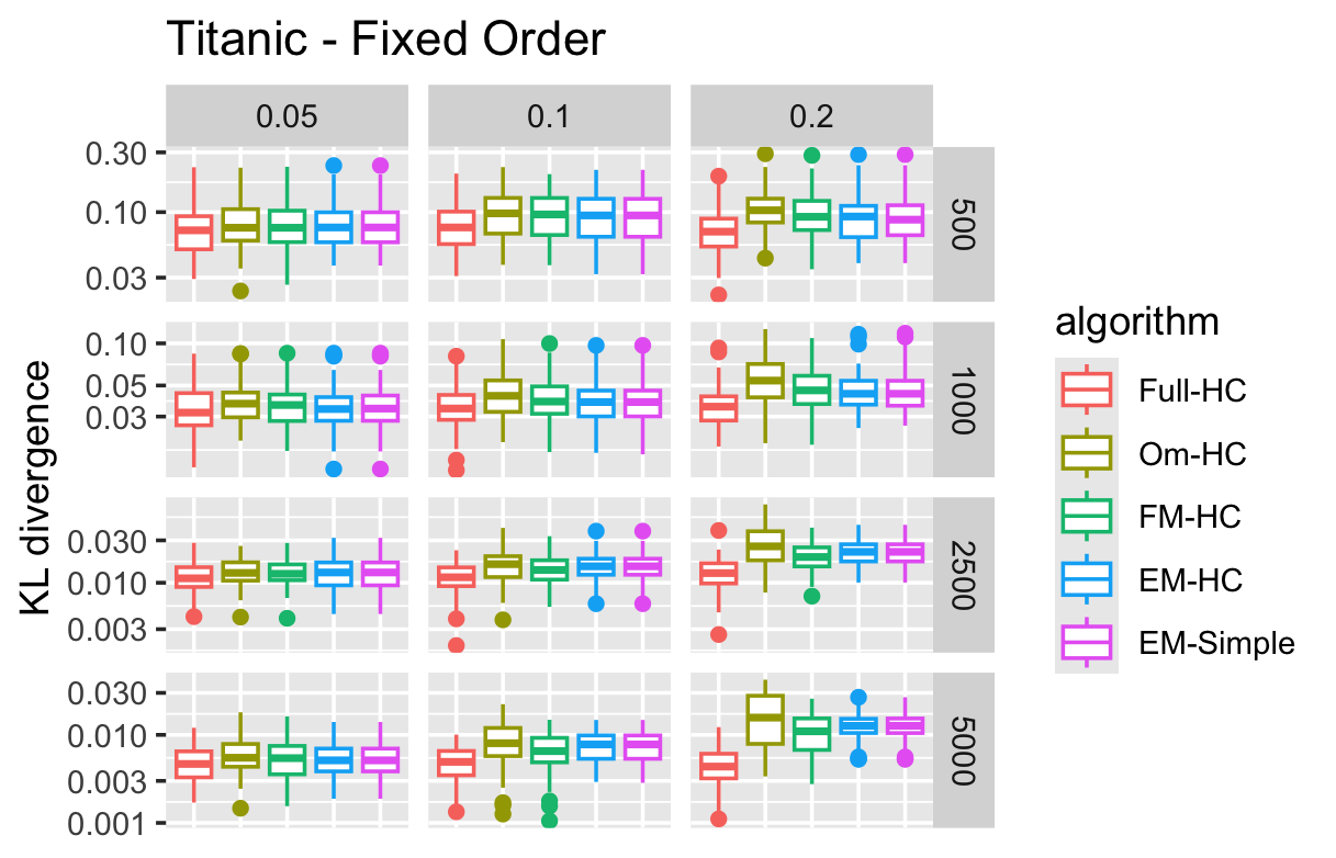
Figure 4: KL divergence for data simulated from the titanic staged tree by missingness proportion and data set size (combining all missingness mechanisms, only HC algorithms).

fig:life-ciao

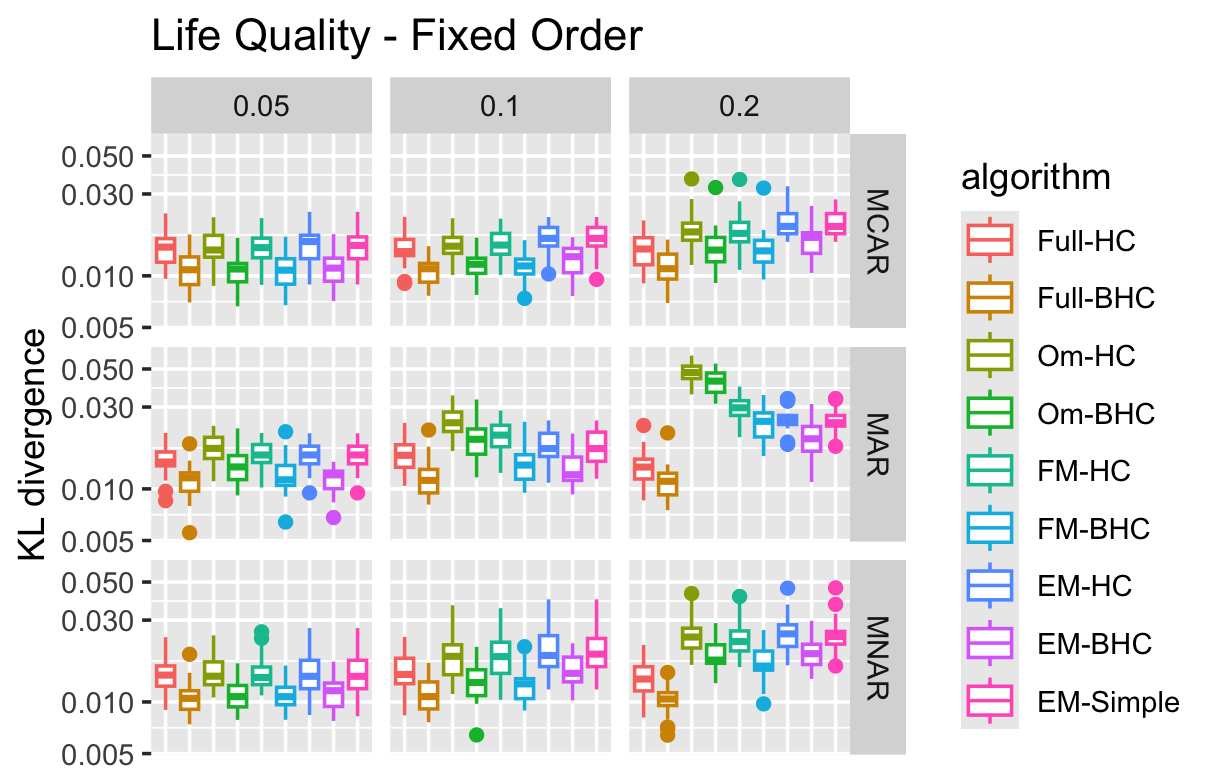
Figure 5: KL divergence for N = 5000 data simulated from the life quality staged tree by missingness proportion and mechanism.

fig:life-ciao2

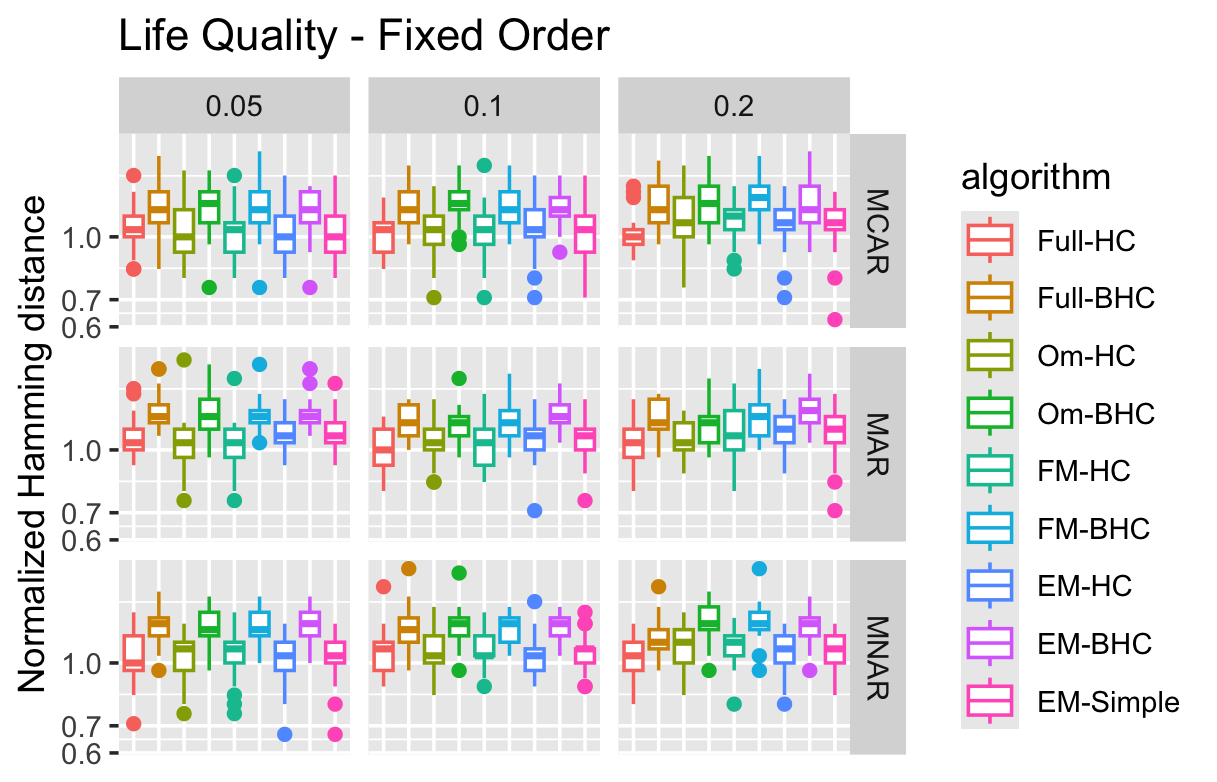
Figure 6: Normalized Hamming distance for N = 5000 data simulated from the life quality staged tree by missingness proportion and mechanism.

fig:coro-hamming

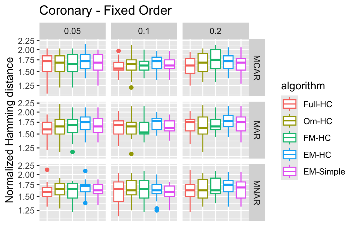
Figure 7: Normalized Hamming distance for N = 5000 data simulated from the coronary staged tree by missingness proportion and mechanism.

fig:bank-kl

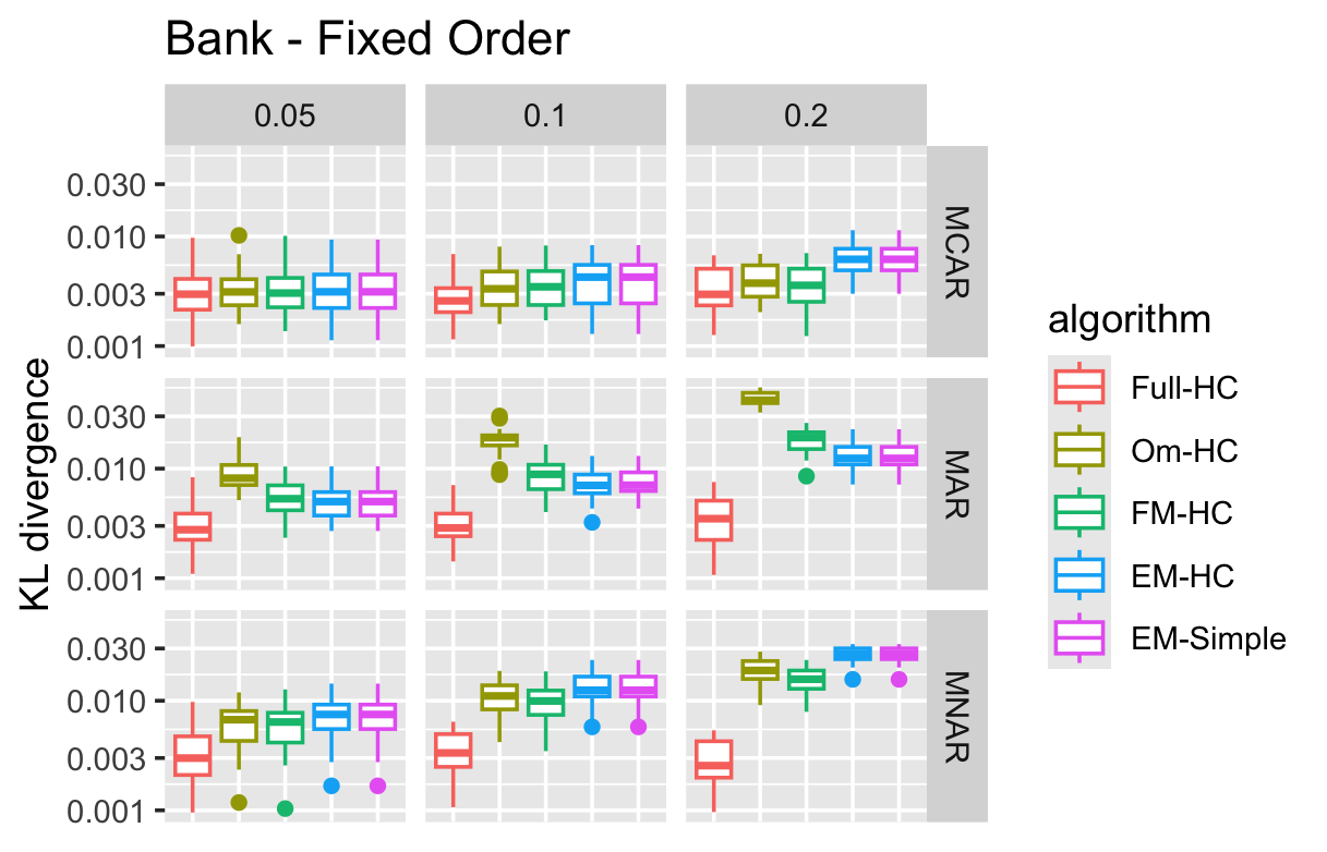
Figure 8: KL divergence for N = 5000 data simulated from the bank staged tree by missingness proportion and mechanism.

fig:bank-cd

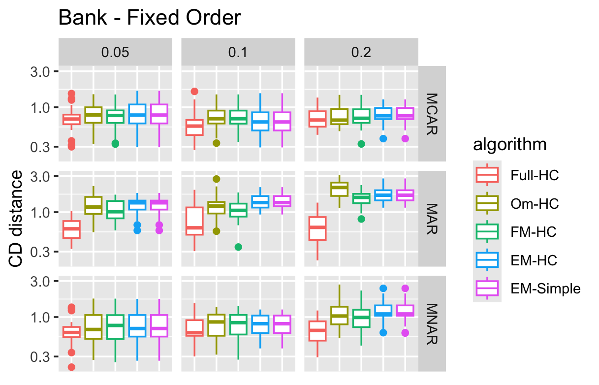
Figure 9: CD distance for N = 5000 data simulated from the bank staged tree by missingness proportion and mechanism.

fig:titanic-cd

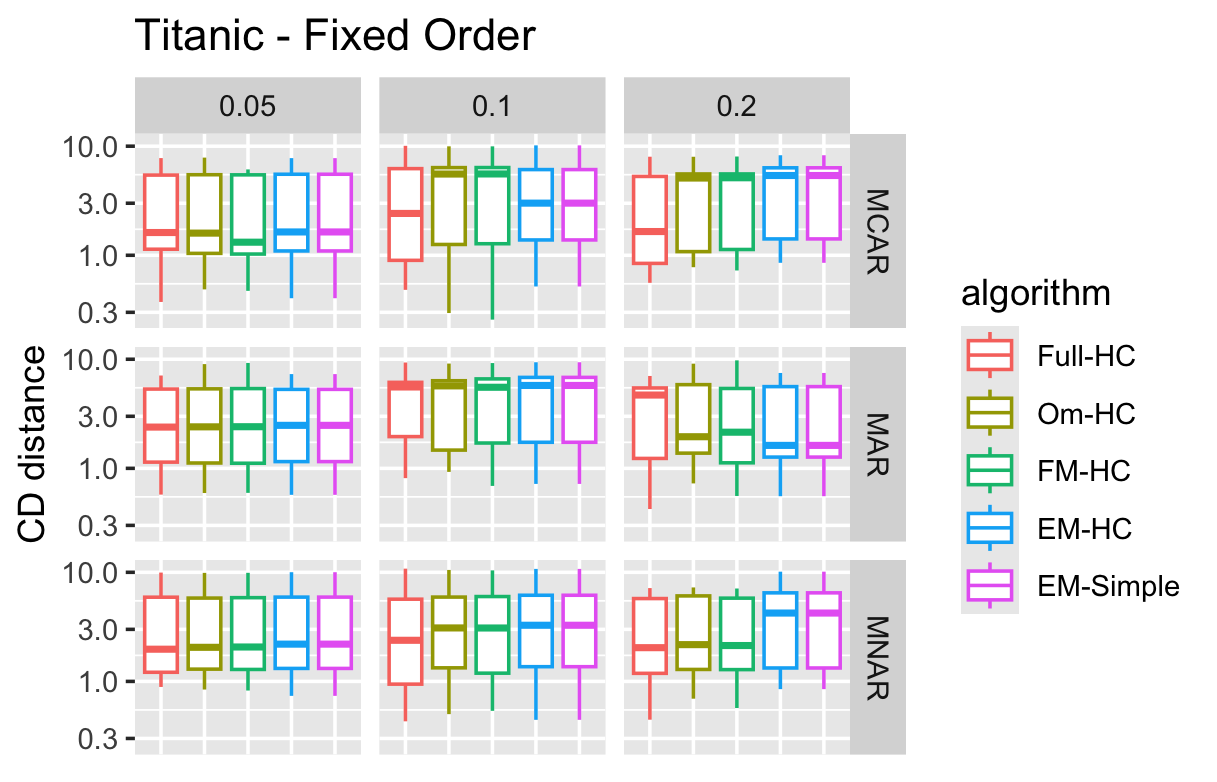
Figure 10: CD distance for N = 5000 data simulated from the titanic staged tree by missingness proportion and mechanism.

fig:chds-kendall

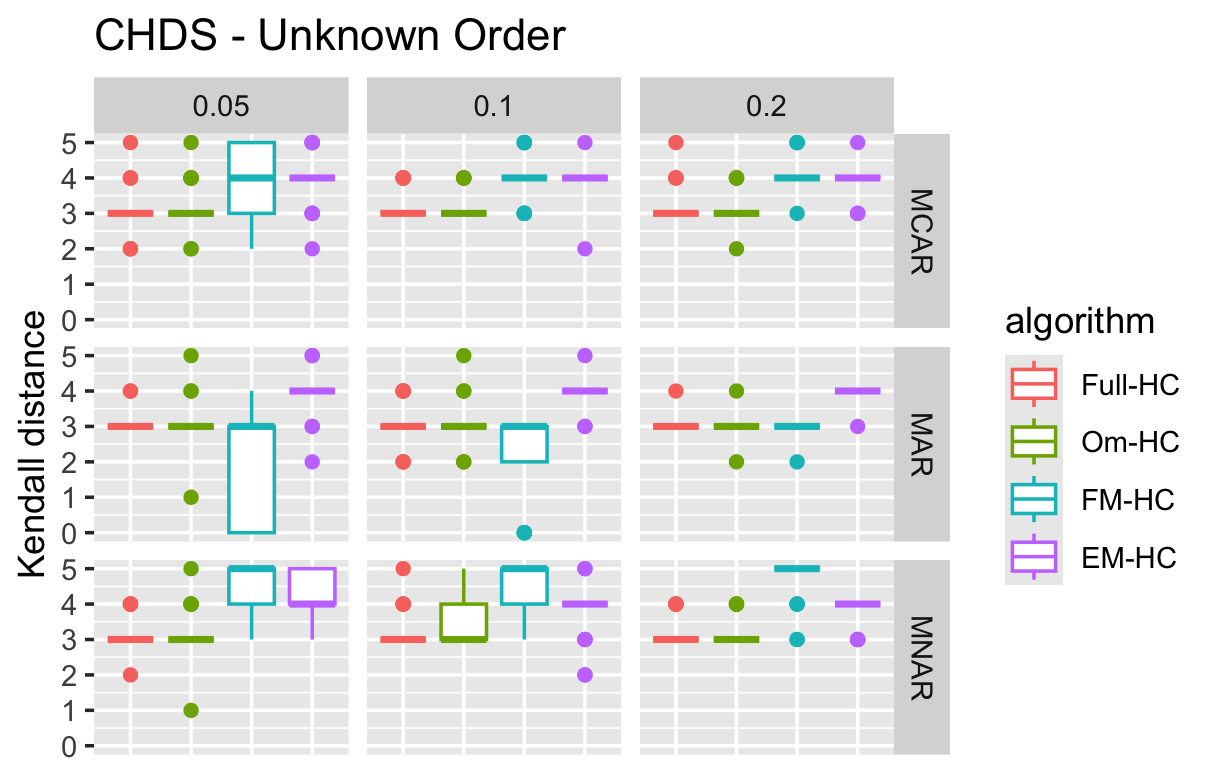
Figure 11: Kendall distance for N = 5000 data simulated from the chds staged tree by missingness proportion and mechanism.

fig:life-kendall

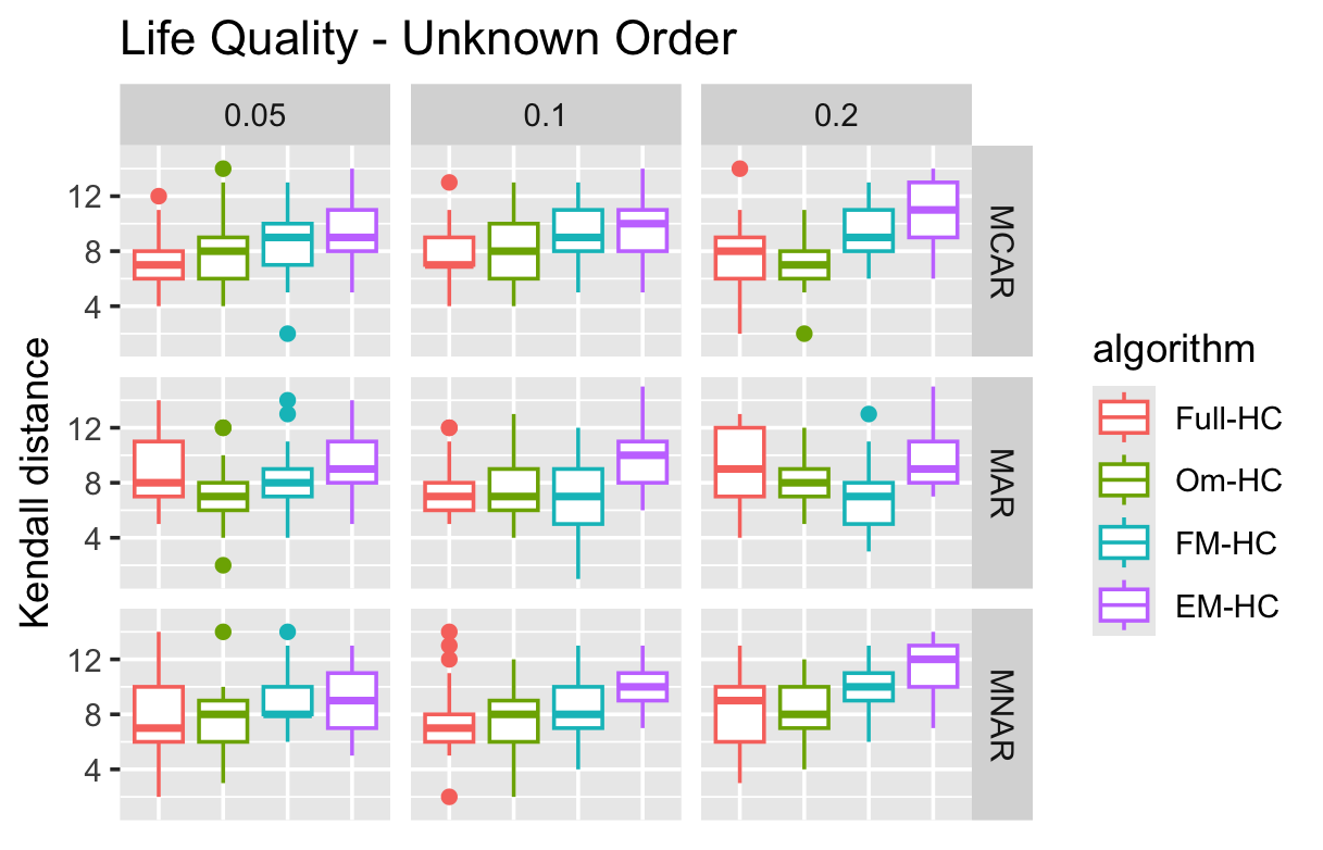
Figure 12: Kendall distance for N = 500 data simulated from the life quality staged tree by missingness proportion and mechanism.

fig:titanic-kll

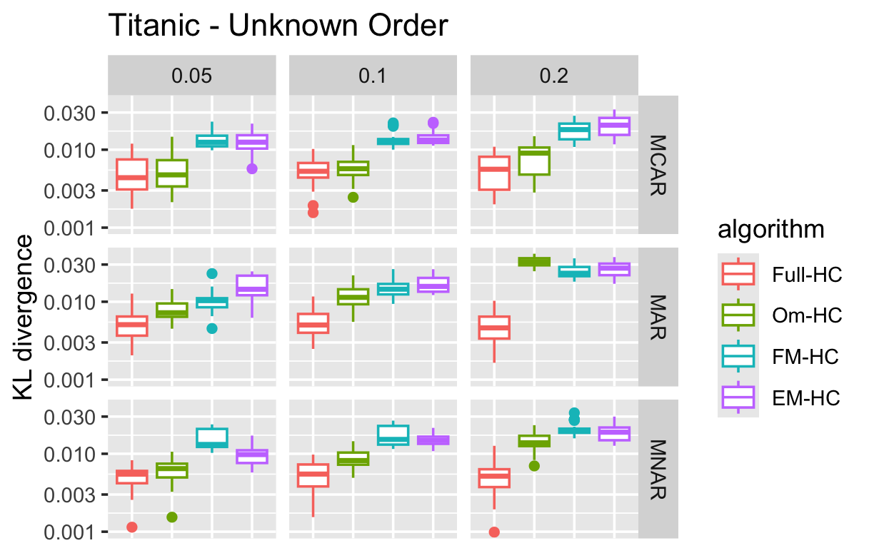
Figure 13: KL divergence for N = 5000 data simulated from the titanic staged tree by missingness proportion and mechanism.

fig:bank-cdd

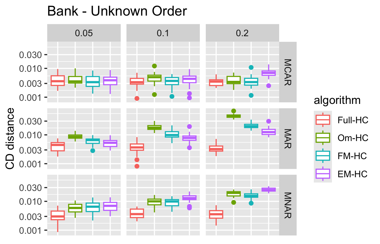
Figure 14: CD distance for N = 5000 data simulated from the bank staged tree by missingness proportion and mechanism.

fig:coronary-time

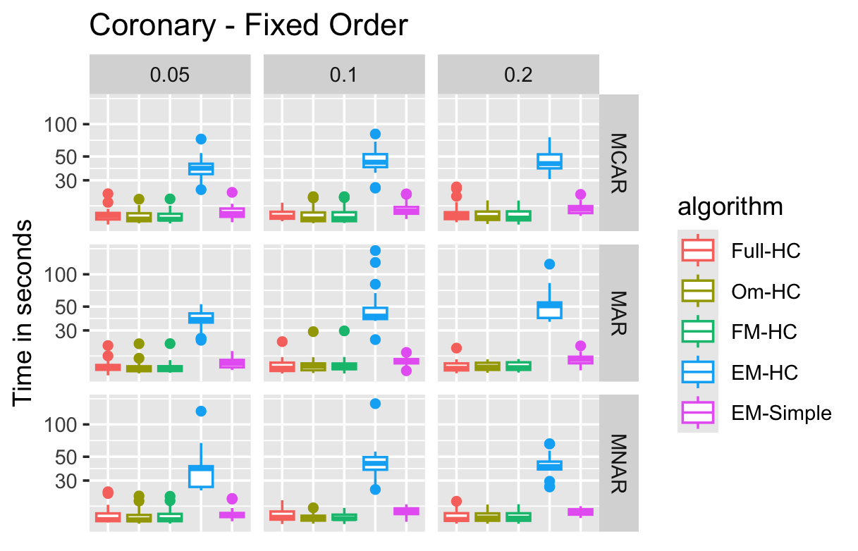
Figure 15: Learning time for N=5000 data simulated from the coronary staged tree by missingness proportion and mechanism.

fig:chds-time1

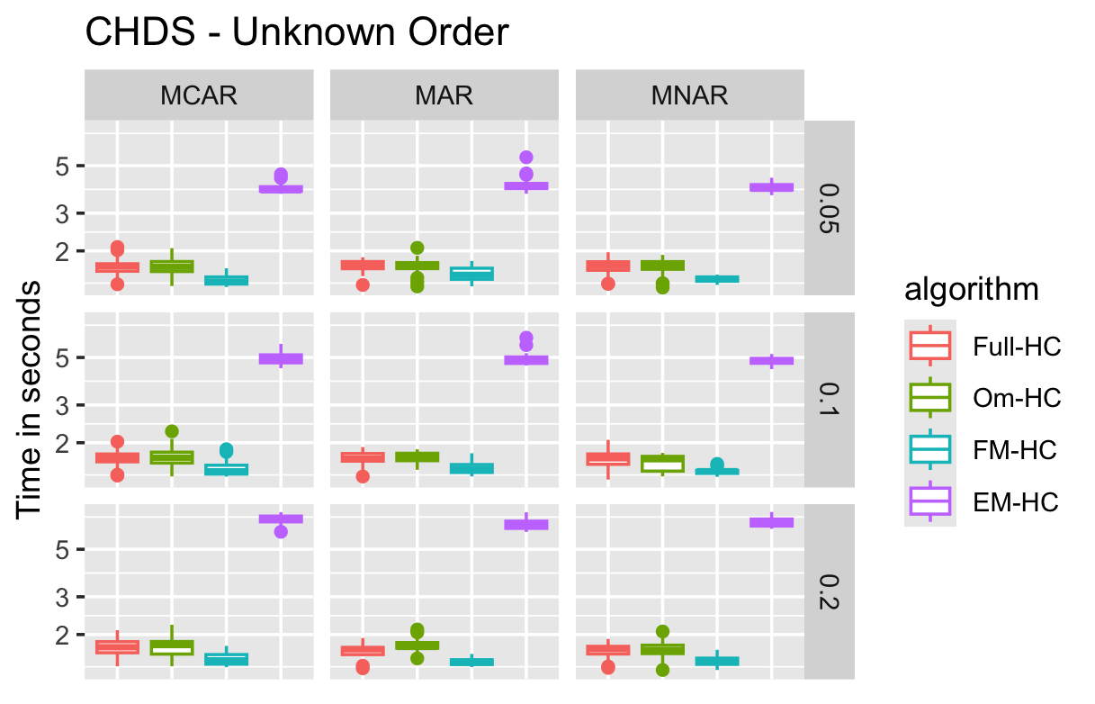
Figure 16: Learning time for N=5000 data simulated from the chds staged tree by missingness proportion and mechanism.

fig:life-time1

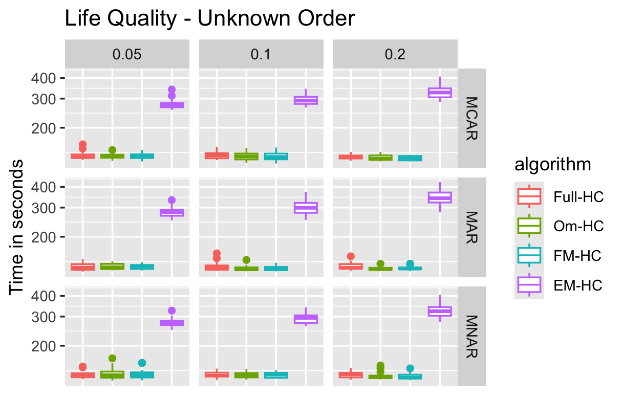
Figure 17: Learning time for N=500 data simulated from the life quality staged tree by missingness proportion and mechanism.

References

- Balov (2013) N. Balov. Consistent model selection of discrete Bayesian networks from incomplete data. Electronic Journal of Statistics, 7:1047–1077, 2013.
- Barclay et al. (2013) L. M. Barclay, J. L. Hutton, and J. Q. Smith. Refining a Bayesian network using a chain event graph. International Journal of Approximate Reasoning, 54(9):1300–1309, 2013.
- Barclay et al. (2014) L. M. Barclay, J. L. Hutton, and J. Q. Smith. Chain event graphs for informed missingness. Bayesian Analysis, 9(1):53–76, 2014.
- Barclay et al. (2015) L. M. Barclay, R. A. Collazo, J. Q. Smith, P. A. Thwaites, and A. E. Nicholson. The dynamic chain event graph. Electronic Journal of Statistics, 9:2130–2169, 2015.
- Bodewes and Scutari (2021) T. Bodewes and M. Scutari. Learning Bayesian networks from incomplete data with the node-average likelihood. International Journal of Approximate Reasoning, 138:145–160, 2021.
- Carli et al. (2022) F. Carli, M. Leonelli, E. Riccomagno, and G. Varando. The R package stagedtrees for structural learning of stratified staged trees. Journal of Statistical Software, 102:1–30, 2022.
- Carter et al. (2024) J. S. Carter, M. Leonelli, E. Riccomagno, and A. Ugolini. Staged trees for discrete longitudinal data. arXiv preprint arXiv:2401.04297, 2024.
- Cohen and Berchenko (2021) N. Cohen and Y. Berchenko. Normalized information criteria and model selection in the presence of missing data. Mathematics, 9(19):2474, 2021.
- Collazo et al. (2018) R. A. Collazo, C. Görgen, and J. Q. Smith. Chain event graphs. CRC Press, 2018.
- Cowell and Smith (2014) R. G. Cowell and J. Q. Smith. Causal discovery through MAP selection of stratified chain event graphs. Electronic Journal of Statistics, 8:965–997, 2014.
- Dempster et al. (1977) A. P. Dempster, N. M. Laird, and D. B. Rubin. Maximum likelihood from incomplete data via the EM algorithm. Journal of the Royal Statistical Society Series B, 39(1):1–22, 1977.
- Filigheddu et al. (2024) M. T. Filigheddu, M. Leonelli, G. Varando, M. Á. Gómez-Bermejo, S. Ventura-Díaz, L. Gorospe, and J. Fortún. Using staged tree models for health data: Investigating invasive fungal infections by aspergillus and other filamentous fungi. Computational and Structural Biotechnology Journal, 24:12–22, 2024.
- Franzin et al. (2017) A. Franzin, F. Sambo, and B. Di Camillo. bnstruct: an R package for Bayesian network structure learning in the presence of missing data. Bioinformatics, 33(8):1250–1252, 2017.
- Freeman and Smith (2011) G. Freeman and J. Q. Smith. Bayesian MAP model selection of chain event graphs. Journal of Multivariate Analysis, 102(7):1152–1165, 2011.
- Friedman (1997) N. Friedman. Learning belief networks in the presence of missing values and hidden variables. In Proceedings of the 14th International Conference on Machine Learning, pages 125–133. Morgan Kaufmann, 1997.
- Friedman (1998) N. Friedman. The Bayesian structural EM algorithm. In Proceedings of the 14th Conference on Uncertainty in Artificial Intelligence, pages 129–138, 1998.
- Görgen et al. (2015) C. Görgen, M. Leonelli, and J. Q. Smith. A differential approach for staged trees. In 13th European Conference on Symbolic and Quantitative Approaches to Reasoning with Uncertainty, pages 346–355. Springer, 2015.
- Görgen et al. (2018) C. Görgen, A. Bigatti, E. Riccomagno, and J. Q. Smith. Discovery of statistical equivalence classes using computer algebra. International Journal of Approximate Reasoning, 95:167–184, 2018.
- Görgen et al. (2022) C. Görgen, M. Leonelli, and O. Marigliano. The curved exponential family of a staged tree. Electronic Journal of Statistics, 16(1):2607–2620, 2022.
- Hughes et al. (2022) C. Hughes, P. Strong, and A. Shenvi. Score equivalence for staged trees. arXiv preprint arXiv:2206.15322, 2022.
- Klimova and Rudas (2016) A. Klimova and T. Rudas. On the closure of relational models. Journal of Multivariate Analysis, 143:440–452, 2016.
- Klimova and Rudas (2022) A. Klimova and T. Rudas. Hierarchical Aitchison–Silvey models for incomplete binary sample spaces. Journal of Multivariate Analysis, 187:104808, 2022.
- Lauritzen (1995) S. L. Lauritzen. The EM algorithm for graphical association models with missing data. Computational Statistics & Data Analysis, 19(2):191–201, 1995.
- Leonelli (2019) M. Leonelli. Sensitivity analysis beyond linearity. International Journal of Approximate Reasoning, 113:106–118, 2019.
- Leonelli and Varando (2022) M. Leonelli and G. Varando. Highly efficient structural learning of sparse staged trees. In International Conference on Probabilistic Graphical Models, pages 193–204. PMLR, 2022.
- Leonelli and Varando (2023) M. Leonelli and G. Varando. Context-specific causal discovery for categorical data using staged trees. In International Conference on Artificial Intelligence and Statistics, pages 8871–8888. PMLR, 2023.
- Leonelli and Varando (2024a) M. Leonelli and G. Varando. Learning and interpreting asymmetry-labeled DAGs: A case study on COVID-19 fear. Applied Intelligence, 54(2):1734–1750, 2024a.
- Leonelli and Varando (2024b) M. Leonelli and G. Varando. Structural learning of simple staged trees. Data Mining and Knowledge Discovery, pages 1–25, 2024b.
- Little and Rubin (2019) R. J. Little and D. B. Rubin. Statistical analysis with missing data. John Wiley & Sons, 2019.
- Rubin (1976) D. B. Rubin. Inference and missing data. Biometrika, 63(3):581–592, 1976.
- Ruggieri et al. (2020) A. Ruggieri, F. Stranieri, F. Stella, and M. Scutari. Hard and soft EM in Bayesian network learning from incomplete data. Algorithms, 13(12):329, 2020.
- Russell and Norvig (2016) S. J. Russell and P. Norvig. Artificial intelligence: A modern approach. Pearson, 2016.
- Schafer (1999) J. L. Schafer. Multiple imputation: A primer. Statistical Methods in Medical Research, 8(1):3–15, 1999.
- Schouten et al. (2018) R. M. Schouten, P. Lugtig, and G. Vink. Generating missing values for simulation purposes: A multivariate amputation procedure. Journal of Statistical Computation and Simulation, 88(15):2909–2930, 2018.
- Scutari (2010) M. Scutari. Learning Bayesian networks with the bnlearn R package. Journal of Statistical Software, 35:1–22, 2010.
- Scutari (2020) M. Scutari. Bayesian network models for incomplete and dynamic data. Statistica Neerlandica, 74(3):397–419, 2020.
- Shafer (1996) G. Shafer. The art of causal conjecture. MIT press, 1996.
- Silander and Leong (2013) T. Silander and T.-Y. Leong. A dynamic programming algorithm for learning chain event graphs. In 16th International Conference on Discovery Science, pages 201–216. Springer, 2013.
- Smith and Anderson (2008) J. Q. Smith and P. E. Anderson. Conditional independence and chain event graphs. Artificial Intelligence, 172(1):42–68, 2008.
- Thwaites et al. (2008) P. A. Thwaites, J. Q. Smith, and R. G. Cowell. Propagation using chain event graphs. In Proceedings of the Twenty-Fourth Conference on Uncertainty in Artificial Intelligence, pages 546–553, 2008.
- Varando et al. (2024) G. Varando, F. Carli, and M. Leonelli. Staged trees and asymmetry-labeled DAGs. Metrika, pages 1–28, 2024.
- Walley et al. (2023) G. Walley, A. Shenvi, P. Strong, and K. Kobalczyk. cegpy: Modelling with chain event graphs in Python. Knowledge-Based Systems, 274:110615, 2023.
- Yu and Smith (2021) X. Yu and J. Q. Smith. Causal algebras on chain event graphs with informed missingness for system failure. Entropy, 23(10):1308, 2021.