Large disks touching three sides of a quadrilateral

Abstract.

We show that every Jordan quadrilateral $Q\subset\mathbb{C}$ contains a disk $D$ so that $\partial D\cap\partial Q$ contains points of three different sides of $Q$. As a consequence, together with some modulus estimates from Lehto and Virtanen, we offer a short proof of the main result obtained by Chrontsios-Garitsis and Hinkkanen in 2024 and it also improves the bounds on their result.

1. Introduction

By a Jordan quadrilateral $Q=Q(v_{1},v_{2},v_{3},v_{4})\subset\mathbb{C}$, we mean a bounded Jordan domain with four marked points, which we call vertices (and we suppose that they are oriented counter-clockwise). To abbreviate we will refer to them just as quadrilaterals. We denote the Jordan arcs joining these points by $a_{1},b_{1},a_{2}$ and $b_{2}$ as it is indicated in Figure 1. We refer to each pair of non-intersecting sides as opposite sides.

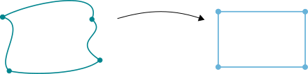
Figure 1. Representation of the vertices, $a$-sides and $b$-sides of a quadrilateral Q, together with it’s representation via conformal mapping to a rectangle.

In this paper we prove:

Theorem 1.1.

For any Jordan quadrilateral $\Omega$, there exists a disk $D\subset\Omega$ so that $\partial D\cap\partial Q$ contains points of three sides of $Q$. In particular, it contains points from opposite sides.

Here the number three is obviously sharp. For instance, in any rectangle that is not a square. If we have a crescent we can also have at most three, with two of them being the endpoints of a pair of adjacent sides, as it can be seen in Figure 2.

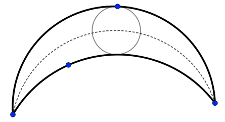
Figure 2. Example of a quadrilateral showing that the number 3 in Theorem 1.1 is sharp, where the figure corresponds to a crescent. The medial axis, which will be defined later in this section, is represented by the dotted curve.

We define as the internal distances between the $a$-sides of $Q$ as

$$s_{a}(Q)\coloneqq\inf\{\textrm{length}(\gamma)\colon\gamma\subset Q\textrm{ Jordan arc joining opposide }a\textrm{-sides}\},$$ (1.1)

and we similarly define $s_{b}(Q)$.

A quadrilateral can be conformally mapped to a rectangle so that the vertices are mapped to the vertices (see 6.2.3 in [1] or 1.2.4 in [11]). The ratio between the length of the $a$-side and the $b$-side of this rectangle is a conformal invariant. We call the quantity $M=M(Q)$ given as in Figure 1 the modulus of $Q$.

The notion of quasiconformal mapping was introduced by H. Grötzsch in 1928. Since the modulus is a conformal invariant, there is no conformal map that maps a square to a rectangle (which is not a square) mapping vertices to vertices. Grötzsch wanted to find the most nearly conformal mapping that satisfied that. There are several (equivalent) definitions of planar quasiconformal mappings (see for example [2, 11]). We say that an orientation preserving homeomorphism $\phi\colon\Omega\subset\mathbb{C}\to\Omega^{{}^{\prime}}\subset\mathbb{C}$ is $K$-quasiconformal if for every quadrilateral $Q\subset\Omega$, we have

$$M(\phi(Q))\leq KM(Q).$$

We use Theorem 1.1 to give an alternative proof of the following result of Chrontsios-Garitsis and Hinkkanen in Section 4.

Corollary 1.2 (Theorem 1.1 in [7]).

For every $K\geq 1$ there is a constant $\delta\in(0,1)$ depending only on $K$ such that every Jordan quadrilateral $Q$ with $M(Q)\in[1/K,K]$ contains a disk of radius $\delta\max\{s_{a}(Q),s_{b}(Q)\}$.

The notion of modulus of a quadrilateral is closely related to what is commonly known as modulus of a path family. By a path family $\Gamma$ we mean a family of curves in $\mathbb{C}$, where each $\gamma\in\Gamma$ is locally rectifiable. We define the modulus of this path family as

$$M(\Gamma)\coloneqq\inf_{\rho\textrm{ admissible}}\int_{Q}\rho^{2}dm(z),$$ (1.2)

where we say a non-negative Borel function $\rho$ is admissible if

$$A(\rho)\coloneqq\int_{\mathbb{C}}\rho^{2}dm<\infty\quad\textrm{ and }\quad L(\rho)\coloneqq\inf_{\gamma\in\Gamma}\int_{\gamma}\rho|dz|\geq 1.$$

The modulus is a conformal invariant. Moreover, if we define the path family $\Gamma$ to consist of all those locally rectifiable paths joining opposite $a$-sides of a quadrilateral $Q$, then the modulus of this path family agrees with the modulus of the quadrilateral, i.e. $M(\Gamma)=M(Q)$.

Our approach to Theorem 1.1 is based on using properties of the medial axis. Given any open proper subset $\Omega$ of $\mathbb{R}^{n}$, we define the medial axis as

$$MA(\Omega)=\{z\in\Omega\colon\exists\textrm{ distinct }w,w^{\prime}\in\partial\Omega\textrm{ s.t. }d(z,w)=d(z,w^{\prime})=d(z,\partial\Omega)\},$$

i.e. it consists of the centers of balls contained in $\Omega$ so that they intersect $\partial\Omega$ in more than one point.

Theorem 1.1 proves that the medial axis of a Jordan domain $\Omega\subset\mathbb{C}$ is always non-empty, since for any choice of four distinct points in $\partial\Omega$ there is a disk $D$ so that $\partial D\cap\partial Q$ contains points of three different sides of $Q$, and in particular of two disjoint sides of $Q$, i.e. it contains more than one point. In a much greater generality than what we cover in this document, i.e. for bounded open proper subsets $\Omega\subset\mathbb{R}^{n}$, in [9] Fremlin shows that the medial axis is an $F_{\sigma}$ set of Hausdorff dimension at most $n-1$ and that $MA(\Omega)$ is connected if and only if $\Omega$ is. For a simply connected planar domain $\Omega\subset\mathbb{C}$, he shows show that in addition it is a union of countably many rectifiable arcs. In this case, in [8] Erdös previously proved the bound on the Hausdorff dimension mentioned before. The medial axis is a subset of the central set of $\Omega$, which is the set of the centers of the maximal balls contained in $\Omega$. In [5] Bishop and Habokyan prove that this set can have Hausdorff dimension arbitrarily close to $2$, even though the medial axis can have Hausdorff dimension at most $1$.

Choi, Choi and Moon characterized in [6] the medial axis of a Jordan domain $\Omega\subset\mathbb{C}$ so that $\partial\Omega$ is a finite union of analytic arcs. In the case where $\partial\Omega$ is a finite union of line segments, the medial axis consists of a finite union of analytic arcs each of which is either a line segment or a parabola.

The medial axis has been proved to be useful in the literature. We cite some references in which this set has been proved to be useful in complex analysis; in [4] Bishop uses the medial axis to compute the conformal map in linear time, and in [3] he uses it to find a tree-like decomposition of any simply-connected domain into Lipschitz domains, improving a previously known result by Jones [10].

The proof of Theorem 1.1 is structured as follows. In Section 2 we show in Lemma 2.4 that if the result is true for a sequence of quadrilaterals converging from inside to a quadrilateral $Q$, then it is also true for $Q$. We also prove in Lemma 2.3 that any quadrilateral $Q$ is a limit from inside of a sequence of quadrilaterals $\{Q_{n}\}$ so that each $\partial Q_{n}$ is a finite union of line segments that make an angle of $\pi/2$ radians at each one of the vertices.

In [6, 9] it is proved that the medial axis of a bounded quadrilateral is connected. In Section 3 we use this fact to prove Theorem 1.1, together with the results from Section 2.

In Section 4, we prove Corollary 1.2 as an application of Theorem 1.1.

Acknowledgments

I would like to thank Chris Bishop for his continued guidance and support, and for reading early drafts of the paper which improved the presentation via his comments and corrections. I would also like to thank Dimitrios Ntalampekos for his comments and corrections, which also improved the presentation.

2. Preliminaries

Given any quadrilateral $Q$ we will approximate it first with a sequence of quadrilaterals $Q_{n}$ from inside, so that they satisfy Theorem 1.1. We then prove that this convergence allows us to conclude that the original quadrilateral also has such a disk so that the boundary intersects the boundary of $Q$ on three sides.

Definition 2.1 (Convergence from inside).

We say that a sequence of quadrilaterals $\{Q_{n}\}$ with sides $a_{j}^{n},b_{j}^{n}$ for $j=1,2$ converge to the quadrilateral $Q$ from inside if

1. $\overline{Q_{n}}\subset\overline{Q}$ for all $n$.

2. For all $\varepsilon>0$, there exists $n_{\varepsilon}$ so that for $n\geq n_{\varepsilon}$ and $j\in\{1,2\}$, the Hausdorff distance (see p. 280-281 in [12]) between $a_{j}^{n}$ (resp. $b_{j}^{n}$) and $a_{j}$ (resp. $b_{j}$) is less than $\varepsilon$.

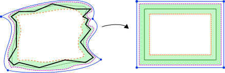
Figure 3. Approximation of any quadrilateral $Q$ from inside via polygons as in Lemma 2.3. The dashed curves represent the quadrilaterals converging from inside to $Q$, whereas the thick curve represents the polygon obtained in Lemma 2.3.

Convergence from inside implies convergence of the corresponding modulus, as we see in Lemma 2.2. The proof is the same as in [11], which we include in this document for completeness.

Lemma 2.2 (Lemma 4.3, p.26 in [11]).

If a sequence of quadrilaterals $Q_{n}$ converges from inside to the quadrilateral $Q$, then $M(Q_{n})\to M(Q)$.

Proof.

Take $\varphi\colon Q\to R$ conformal as in Figure 1, then $\varphi$ is uniformly continuous in $Q$, thus the sequence of quadrilaterals $\varphi(Q_{n})$ converges from inside to the quadrilateral $\varphi(Q)=R$. This means that for $\varepsilon>0$ small enough we have $s_{a}(\varphi(Q_{n}))\geq 1-2\varepsilon$ and $s_{b}(\varphi(Q_{n}))\geq M(Q)-2\varepsilon$. Also, $m(\varphi(Q_{n}))\leq m(\varphi(Q))=M(Q)$. Therefore, if in (1.2) we take the Euclidean metric normalized so that it is admissible, we have

$$\frac{\left(M(Q)-2\varepsilon\right)^{2}}{M(Q)}\leq M(\varphi(Q_{n}))\leq\frac{M(Q)}{\left(1-2\varepsilon\right)^{2}}.$$

Since $M(\varphi(Q_{n}))=M(Q_{n})$, we see that as $\varepsilon\to 0$, then $M(Q_{n})\to M(Q)$. ∎

Lemma 2.2 also provides a way to regard any quadrilateral $Q$ as a limit from inside of, for example, analytic quadrilaterals or polygonal quadrilaterals. More precisely, we have the following result, where by vertices we mean vertices of the quadrilateral and not the vertices of the polygon.

Lemma 2.3.

Any quadrilateral $Q$ is a limit from inside of a nested sequence of quadrilaterals $Q_{n}$ so that the sides of each one of the $Q_{n}$ is a finite union of non-trivial line segments. Moreover, the two segments that meet at the vertices of each one of the quadrilaterals $Q_{n}$ form an angle of $\pi/2$ radians.

Proof.

Let $\varphi\colon Q\to R$ be conformal, where $R$ is a rectangle with vertices $0,M,i$ and $M+i$. Define $R_{n}=\{z\in R\colon d(z,\partial R)\geq 1/n\}$ for $n\in\mathbb{N}$. Then $R_{n}$ is a compact subset of $R$ and the sequence of quadrilaterals $\{R_{n}\}_{n\in\mathbb{N}}$ converges to the quadrilateral $R$ from inside, where we are taking as the vertices of this quadrilaterals the corners of the rectangles. Therefore, the sequence $\{\varphi^{-1}(R_{n})\}$ converges to $Q$ from inside.

We now obtain the sequence of polygons that approximates $Q$ from inside. Approximate each $\varphi^{-1}(\partial R_{2n})$ via a polygonal Jordan curve (see for example Lemma 2 in [13]) that it is contained in $\varphi^{-1}(\overline{R_{2n+1}}\setminus R_{2n-1})$ so that at each one of the vertices of the approximating quadrilaterals (not the vertices from the polygon) it has an angle of $\pi/2$ radians, as it has been illustrated in Figure 3. We define $Q_{n}$ as the interior of the polygonal Jordan curve, which is a quadrilateral. Also, if two adjacent line segments of this approximation are part of the same line, we consider them as the same line segment. This new sequence of quadrilaterals $\{Q_{n}\}_{n\in\mathbb{N}}$ converges to $Q$ from inside by construction. ∎

Next we will show that if Theorem 1.1 holds for a sequence of quadrilaterals that converge from inside to a quadrilateral $Q$, then the same holds for $Q$.

Lemma 2.4.

Let $Q$ be a quadrilateral and suppose that $Q_{n}$ is a increasing sequence of quadrilaterals of definite modulus converging to $Q$ from inside. If every $Q_{n}$ has a disk $D_{n}$ so that $\partial Q_{n}\cap\partial D_{n}$ contains points of three sides of $Q_{n}$, then the same holds for $Q$.

Proof.

Let $D_{n}=D(c_{n},r_{n})$ be the sequence of corresponding disks. By passing to a subsequence and changing the labeling of the sides of $Q$ if necessary, we can suppose that their boundary circles all have points in opposite $a$-sides and from the side $b_{1}$. Observe that:

1. $\textrm{diam}(Q)\geq\textrm{diam}(Q_{n})\geq 2r_{n}\geq s_{a}(Q_{n})$, and $s_{a}(Q_{n})\to s_{a}(Q)>0$. So $\{r_{n}\}$ is a bounded sequence, bounded below away from $0$.

2. Given $\varepsilon>0$ small enough, there exists $N$ so that for $n\geq N$ we have $c_{n}\in\{z\in Q\colon\textrm{dist}(z,\partial Q)\geq(s_{a}(Q)-\varepsilon)/2\}=K_{\varepsilon}$, which is a compact set. Observe that if $\varepsilon^{\prime}<\varepsilon$, then $K_{\varepsilon}\supset K_{\varepsilon^{\prime}}$.

3. For each $D_{n}=D(c_{n},r_{n})$ we have at least points $p_{n}\in a_{1}^{n}$, $q_{n}\in a_{2}^{n}$ and $w_{n}\in b_{1}^{n}$, where $a_{1}^{n}$ is the $a_{1}$ side of $Q_{n}$, $a_{2}^{n}$ is the $a_{2}$ side of $Q_{n}$ and $b_{1}^{n}$ is the $b_{1}$ side of $Q_{n}$.

Take a subsequence so that $c_{n_{j}},r_{n_{j}},p_{n_{j}},q_{n_{j}},w_{n_{j}}$ converge to $c\in K_{\varepsilon},r>0,p\in a_{1},q\in a_{2}$ and $w\in b_{1}$ (now referring to the corresponding sides of $Q$). Then the disk $D=D(c,r)$ is contained in $Q$ and $\{p,q,w\}\subset\partial D\cap\partial Q$, which are points of three sides of $Q$. ∎

Observe that in the previous Lemma we are not excluding the possibility of $w$ being equal to either $p$ or $q$. This is the case, for example, if we have a crescent, as it can be seen in Figure 2.

3. Proof of the main theorem

By Lemma 2.3, given any quadrilateral we can build a sequence of quadrilaterals $Q_{n}$, so that $\partial Q_{n}$ is a finite union of non-trivial line segments, with the two segments meeting at each one of the vertices making an angle of $\pi/2$ radians. By Lemma 2.4, if we show that Theorem 1.1 holds for such quadrilaterals, then the Theorem is proved. This is what we show in Proposition 3.1.

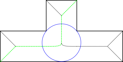
Figure 4. Illustration of the proof of Proposition 3.1. The medial axis is the union of the dashed curves. The circle has its center in the medial axis. The continuous path $\gamma$ joining $v_{1}$ and $v_{3}$ within the medial axis is represented in a lighter color.

Proposition 3.1.

Let $Q=Q(v_{1},v_{2},v_{3},v_{4})$ be a polygonal quadrilateral so that $\partial Q$ is a finite union of non-trivial line segments that form an angle of $\pi/2$ radians at each one of the vertices $v_{j}$. Then, there is a continuous path of disks $\gamma$ from $[0,1]$ to the set of all disks $D(c,r)\subset Q$, with the product topology as a subset of $\overline{Q}\times[0,diam(Q)]$, so that

1. $\gamma(0)=\{v_{1}\}$ and $\gamma(1)=\{v_{3}\}$, where we consider $\{v_{j}\}$ as a disk of radius $0$ and center $v_{j}$.

2. For each $s\in(0,1)$, the circle $\partial\gamma(s)$ intersects the two connected components of $Q\setminus\{v_{1},v_{3}\}$.

3. There exists $s^{*}\in(0,1)$ so that $\gamma(s^{*})=D\subset Q$ is such that $\partial D\cap\partial Q$ contains points of three sides of the quadrilateral $Q$.

Proof.

Both (a) and (b) follow from the path connectedness of the medial axis (see Theorem 2D in [9] or Theorem 7.3 in [6]), together with having an angle of $\pi/2<\pi$ radians at each one of the vertices of our quadrilateral, which guarantees that each one of the vertices is a limit point of the medial axis of $Q$. This is represented in Figure 4. To prove (c), take a path of disks connecting the vertices $v_{1}$ and $v_{3}$ of $Q$, contained in the medial axis of $Q$ . We know that this path is a finite union of analytic arcs by Theorem 7.1 in [6] (in fact, in this case each analytic arc is either a line segment or a parabola). Close to $v_{1}$, the maximal disks around those points intersect the two line segments that are adjacent to $v_{1}$ (by the $\pi/2$ angle), and in particular, to the two adjacent sides of the quadrilateral to $v_{1}$. Close to $v_{3}$, by the $\pi/2$ angle, the maximal disks around those points intersect the two line segments that are adjacent to $v_{3}$. Since we have a continuous path joining those points, there is one last point for which these maximal disks intersect the two sides of the quadrilateral $Q$ that are adjacent to $v_{1}$. At that point, the maximal disk also intersects one of the other two sides of $Q$. ∎

Observe that Proposition 3.1 (c) is precisely the particular case of Theorem 1.1 for the quadrilaterals obtained in Lemma 2.3. Therefore, by Lemma 2.4, Theorem 1.1 is proved. ∎

4. Proof of Corollary 1.2

The characterization of the modulus in (1.2) leads to many interesting applications. It yields bounds on the modulus provided that we know some geometric properties of the quadrilateral by choosing adequate admissible metrics. For example, in [11] Lehto and Virtanen prove the following:

Proposition 4.1 (Lemma 4.1, p. 23 in [11]).

The modulus of a quadrilateral $Q$ satisfies the following double inequality

$$\frac{\left(\log(1+2s_{b}(Q)/s_{a}(Q))\right)^{2}}{\pi+2\pi\log(1+2s_{b}(Q)/s_{a}(Q))}\leq M(Q)\leq\frac{\pi+2\pi\log(1+2s_{a}(Q)/s_{b}(Q))}{\left(\log(1+2s_{a}(Q)/s_{b}(Q))\right)^{2}},$$

where $s_{a}(Q)$ and $s_{b}(Q)$ are defined as in (1.1).

Observe that Proposition 4.1 shows that having a family of quadrilaterals $Q$ with uniformly bounded modulus $M(Q)\in[1/K,K]$ is equivalent to having a uniformly bounded ratio between the internal distances, that is, $s_{a}(Q)/s_{b}(Q)\in[1/L,L]$, where $L$ depends only on $K$.

Let’s see how Theorem 1.1 implies Corollary 1.2. Let $C$ the boundary of the disk given by Theorem 1.1, as it is represented in Figure 5. Then, there is a segment $\gamma$, contained in the interior of $C$, joining opposite sides, which we can suppose it is joining the $a$-sides. We have $\textrm{diam}(C)\geq\textrm{length}(\gamma)\geq s_{a}(Q)$. Thus there exists a disk with radius $s_{a}(Q)/2$ contained in $Q$. Since we are considering quadrilaterals with uniformly bounded modulus, then by Proposition 4.1,

$$s_{a}(Q)\geq s_{b}(Q)/L.$$

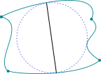
Figure 5. Representation of the circle obtained in Theorem 1.1 that intersects three sides of our quadrilateral $Q$.

That is, it also contains a disk of radius $s_{b}(Q)/2L$. Therefore, our quadrilateral $Q$ contains a disk of radius $\delta\max\{s_{a}(Q),s_{b}(Q)\}$, where $\delta=1/2L\in(0,1)$ and as we have mentioned before, this constant $L$ only depends on the bound $K$ for the modulus.

This completes the proof of Corollary 1.2.

References

- [1] Lars Ahlfors “Complex analysis—an introduction to the theory of analytic functions of one complex variable” Reprint of the 1978 original [ 0510197] AMS Chelsea Publishing, Providence, RI, [2021] ©2021, pp. xiv+331 URL: https://mathscinet.ams.org/mathscinet-getitem?mr=4506522
- [2] Lars V. Ahlfors “Lectures on quasiconformal mappings” With supplemental chapters by C. J. Earle, I. Kra, M. Shishikura and J. H. Hubbard 38, University Lecture Series American Mathematical Society, Providence, RI, 2006, pp. viii+162 DOI: 10.1090/ulect/038
- [3] Christopher J. Bishop “Conformal mapping in linear time” In Discrete Comput. Geom. 44.2, 2010, pp. 330–428 DOI: 10.1007/s00454-010-9269-9
- [4] Christopher J. Bishop “Tree-like decompositions of simply connected domains” In Rev. Mat. Iberoam. 28.1, 2012, pp. 179–200 DOI: 10.4171/RMI/673
- [5] Christopher J. Bishop and Hrant Hakobyan “A central set of dimension 2” In Proc. Amer. Math. Soc. 136.7, 2008, pp. 2453–2461 DOI: 10.1090/S0002-9939-08-09173-9
- [6] Hyeong In Choi, Sung Woo Choi and Hwan Pyo Moon “Mathematical theory of medial axis transform” In Pacific J. Math. 181.1, 1997, pp. 57–88 DOI: 10.2140/pjm.1997.181.57
- [7] Efstathios-Konstantinos Chrontsios-Garitsis and Aimo Hinkkanen “A geometric property of quadrilaterals” In Ann. Fenn. Math. 49.1, 2024, pp. 281–302 URL: https://mathscinet.ams.org/mathscinet-getitem?mr=4735579
- [8] Paul Erdös “Some remarks on the measurability of certain sets” In Bull. Amer. Math. Soc. 51, 1945, pp. 728–731 DOI: 10.1090/S0002-9904-1945-08429-8
- [9] D.. Fremlin “Skeletons and central sets” In Proc. London Math. Soc. (3) 74.3, 1997, pp. 701–720 DOI: 10.1112/S0024611597000233
- [10] Peter W. Jones “Rectifiable sets and the traveling salesman problem” In Invent. Math. 102.1, 1990, pp. 1–15 DOI: 10.1007/BF01233418
- [11] O. Lehto and K.. Virtanen “Quasiconformal mappings in the plane” Translated from the German by K. W. Lucas, Die Grundlehren der mathematischen Wissenschaften, Band 126 Springer-Verlag, New York-Heidelberg, 1973, pp. viii+258 URL: https://mathscinet.ams.org/mathscinet-getitem?mr=344463
- [12] James R. Munkres “Topology” Second edition Prentice Hall, Inc., Upper Saddle River, NJ, 2000, pp. xvi+537 URL: https://mathscinet.ams.org/mathscinet-getitem?mr=3728284
- [13] Helge Tverberg “A proof of the Jordan curve theorem” In Bull. London Math. Soc. 12.1, 1980, pp. 34–38 DOI: 10.1112/blms/12.1.34