1
Context-Specific Refinements of Bayesian Network Classifiers
Abstract
Supervised classification is one of the most ubiquitous tasks in machine learning. Generative classifiers based on Bayesian networks are often used because of their interpretability and competitive accuracy. The widely used naive and TAN classifiers are specific instances of Bayesian network classifiers with a constrained underlying graph. This paper introduces novel classes of generative classifiers extending TAN and other famous types of Bayesian network classifiers. Our approach is based on staged tree models, which extend Bayesian networks by allowing for complex, context-specific patterns of dependence. We formally study the relationship between our novel classes of classifiers and Bayesian networks. We introduce and implement data-driven learning routines for our models and investigate their accuracy in an extensive computational study. The study demonstrates that models embedding asymmetric information can enhance classification accuracy.
keywords:
Classification; Bayesian networks; Staged trees; Structural learning.1 Introduction
We consider the problem of supervised classification of a categorical class variable given a vector of categorical features using generative classifiers. Given a training set of labeled observation , a generative classifier aims to learn a joint probability and assign a non-labeled instance to the most probable a posteriori class found as
where and . With and we denote the sample spaces of the feature and class variables, respectively.
Bayesian network classifiers (BNCs) (Bielza and Larrañaga, 2014; Friedman et al., 1997) are the most widely-used class of generative classifiers which factorize according to a Bayesian network over and . They have been shown to have competitive classification performance with respect to black-box discriminative classifiers while being interpretable and explainable since they explicitly describe the relationship between the features using a simple graph. The famous naive Bayes classifier (Minsky, 1961) can be seen as a specific instance of BNCs with a fixed graph structure where no edges between features are allowed.
The main limitation of BNCs is that they can only formally encode symmetric conditional independence. However, there is now a growing amount of evidence that real-world scenarios are better described by more generic, asymmetric types of relationships (e.g. Eggeling et al., 2019; Leonelli and Varando, 2023, 2024c; Rios et al., 2024), for instance context-specific ones (Boutilier et al., 1996). There have been limited attempts to extend BNCs to embed asymmetric types of dependence, most notably Bayesian multinets (Geiger and Heckerman, 1996), but their use in practice is limited.
Staged tree classifiers have been recently introduced by Carli et al. (2023). They have been shown to extend the class of BNCs to embed complex patterns of asymmetric dependence using staged tree models (Collazo et al., 2018; Smith and Anderson, 2008). Staged trees are an explainable class of probabilistic graphical models that visually depict dependence using a colored tree. A particular type of staged tree classifier is the naive staged tree, which, while having the same complexity as naive Bayes, extends it to account for asymmetric dependences.
In this paper, we introduce novel classes of staged tree classifiers, which can be seen as refinements of famous sub-classes of BNCs, namely TAN (Friedman et al., 1997) and -DB (Sahami, 1996) classifiers. We formally investigate the relationship between our novel staged tree classifiers and their BNCs’ counterparts. Data-driven learning routines for these novel classes are discussed and implemented. An extensive experimental study compares the classification performance of our novel classifiers to BNCs. The results highlight that these novel classes can increase classification accuracy in some cases by explicitly modelling asymmetric and flexible relationships between features.
2 Bayesian Network Classifiers
2.1 The Bayesian Network Model
Let be a directed acyclic graph (DAG) with vertex set and edge set . For , we let and where . We say that is Markov to if, for ,
| (1) |
where is the parent set of in . Henceforth, we assume the existence of a linear ordering of for which only pairs where appears before in the order can be in the edge set.
The ordered Markov condition implies conditional independences of the form
| (2) |
Let be a DAG and Markov to . The Bayesian network model (associated to ) is
where is the ()-dimensional probability simplex.
Let be the set of DAGs with vertex set and ordering . We define the space of Bayesian network models over as
2.2 Classes of Bayesian Network Classifiers
BNCs are BNs with vertices and . Although any Bayesian network could be, in principle, used for classification, most commonly, the space of considered DAGs is restricted to those where has no parents and there is an edge from to for every (this class is sometimes referred to as Bayesian network-augmented naive Bayes, Friedman et al., 1997). By BNCs, we henceforth refer to such classifiers.
Subclasses of BNCs entertaining specific properties in the underlying DAG have been defined. The simplest possible model is the so-called naive Bayes classifier (Minsky, 1961), which assumes that the features are conditionally independent, given the class (\figurereffig:naivebnc). BNCs of increasing complexity can then be defined by adding dependencies between the feature variables. Another commonly used classifier is the TAN BNC (Friedman et al., 1997), for which each feature has at most two parents: the class and possibly another feature (\figurereffig:tanbnc). The more generic -DB BNCs (Sahami, 1996) assume that each feature can have at most feature parents (\figurereffig:kdepbnc). Naive and TAN classifiers are -DB BNCs for and , respectively.
fig:bncs
Although BNCs of any complexity can be learned and used in practice, empirical evidence demonstrates that model complexity does not necessarily imply better classification accuracy (Bielza and Larrañaga, 2014). Despite their simplicity, naive and TAN BNCs have been shown to lead to good accuracy in classification problems.
3 Staged Tree Classifiers
3.1 The Staged Tree Model
Consider a -dimensional random vector taking values in the product sample space . Let be a directed, finite, rooted tree with vertex set , root node , and edge set . For each , let be the set of edges emanating from and be a set of labels.
An -compatible staged tree is a triple , where is a rooted directed tree and:
-
1.
;
-
2.
For all , if and only if and , or and for some ;
-
3.
is a labeling of the edges such that for some function . The function is called the coloring of the staged tree .
If then and are said to be in the same stage. Therefore, the equivalence classes induced by form a partition of the internal vertices of the tree in stages.
Points 1 and 2 above construct a rooted tree where each root-to-leaf path, or equivalently each leaf, is associated with an element of the sample space . Then a labeling of the edges of such a tree is defined where labels are pairs with one element from a set and the other from the sample space of the corresponding variable in the tree. By construction, -compatible staged trees are such that two vertices can be in the same stage if and only if they correspond to the same sample space.
fig:sts
fig:compst reports an -compatible staged tree over three binary variables. The coloring given by the function is shown in the vertices and each edge is labeled with . The edge labeling can be read from the graph by combining the text label and the color of the emanating vertex. The staging of the staged tree in \figurereffig:compst is given by the partition , , , and .
The parameter space associated to an -compatible staged tree with labeling is defined as
| (3) |
Equation (3) defines a class of probability mass functions over the edges emanating from any internal vertex coinciding with conditional distributions , and . In the staged tree in \figurereffig:compst the staging implies that the conditional distribution of given , and , represented by the edges emanating from , is equal to the conditional distribution of given and . A similar interpretation holds for the staging . This in turn implies that , thus illustrating that the staging of a tree is associated with conditional independence statements.
Let denote the leaves of a staged tree . Given a vertex , there is a unique path in from the root to , denoted as . The number of edges in is called the distance of , and the set of vertices at distance is denoted by . For any path in , let denote the set of edges in the path .
The staged tree model associated to the -compatible staged tree is the image of the map
| (4) | ||||
Therefore, staged tree models are such that atomic probabilities are equal to the product of the edge labels in root-to-leaf paths and coincide with the usual factorization of mass functions via recursive conditioning.
Let be the set of functions from to , that is all possible partitions, or staging, of the staged tree. We define . So as is the union of all possible BN models given a specific ordering, is the union of all possible staged tree models, that is of all possible stagings, given a specific ordering of the variables.
3.2 Staged Trees and Bayesian Networks
Although the relationship between Bayesian networks and staged trees was already formalized by Smith and Anderson (2008), a formal procedure to represent a Bayesian network as a staged tree has been only recently introduced (e.g. Varando et al., 2024). Assume is topologically ordered with respect to a DAG and consider an -compatible staged tree with vertex set , edge set and labeling defined via the coloring of the vertices. The staged tree , with vertex set , edge set and labeling so constructed, is called the staged tree model of . Importantly, , i.e. the two models are exactly the same, since they entail exactly the same factorization of the joint probability (Smith and Anderson, 2008). Clearly, the staging of represents the Markov conditions associated to the graph .
Varando et al. (2024) approached the reverse problem of transforming a staged tree into a Bayesian network. Of course, since staged trees represent more general asymmetric conditional independences, given a staged tree most often there is no Bayesian network with DAG such that . However, Varando et al. (2024) introduced an algorithm that, given an -compatible staged tree , finds the minimal DAG such that . Minimal means that such a DAG embeds all symmetric conditional independences that are in and that there are no DAGs with less edges than embedding the same conditional independences.
As an illustration, the staged tree in \figurereffig:compst can be constructed as the from the Bayesian network with DAG , embedding the conditional independence . Conversely, consider the staged tree in \figurereffig:xorst. Such a staged tree does not embed any symmetric conditional independence, only non-symmetric ones, and therefore there is no DAG such that . Furthermore, the minimal DAG such that is the complete one since the staging of the tree implies direct dependence between every pair of variables.
Leonelli and Varando (2022) introduced a subclass of staged trees based on the topology of the associated minimal DAG, which will be relevant for the definition of the novel classifiers below. A staged tree is said to be in the class of -parents staged trees if the maximum in-degree in is less or equal to . For instance, the staged tree in \figurereffig:compst is in the class of 1-parent staged trees, whilst the one in \figurereffig:xorst is not, since its associated minimal DAG is such that has two parents.
3.3 Staged Trees for Classification
fig:sts1
Carli et al. (2023) discussed how staged tree models can be used for classification purposes. As in \sectionrefsec:intro, suppose is a vector of features and is the class variable. A staged tree classifier for the class and features is a -compatible staged tree. The requirement of being the root of the tree follows from the idea that in most BNCs the class has no parents, so to maximize the information provided by the features for classification.
All BNCs reviewed in \sectionrefsec:bn can therefore be represented as staged tree classifiers, by constructing the equivalent . \figurereffig:sts1 shows the staged trees equivalent to the BNCs in \figurereffig:bncs. However, Carli et al. (2023) demonstrated that the class of staged tree classifiers is much larger than that of BNCs. Formally, letting be the space of BNCs and the space of -compatible staged trees, then .
Since the class of staged tree classifiers is extremely rich, Carli et al. (2023) introduced a subclass of staged tree classifiers termed naive. Let be the set of nodes of a tree at distance from the root. Formally, a -compatible staged tree classifiers such that for every , the set is partitioned into stages is called naive. The name naive comes from these classifiers having free parameters that need to be learned, the same number as for the standard naive Bayes model. An example of a naive staged tree is given in \figurereffig:naive. Notice that unlike naive BNCs, which have a fixed DAG structure, the coloring of the vertices must also be learned for data for naive staged trees. Carli et al. (2023) proposed using k-means and hierarchical clustering algorithms for this task.
Just as for generic staged tree classifiers, naive staged trees generalize naive BNCs. Letting and be the space of naive BNCs and naive staged tree classifiers, respectively, we have that . Importantly, Carli et al. (2023) showed via simulation experiments that naive staged tree classifiers can correctly classify parity functions (or 2-XORs), which cannot be captured by naive Bayes models (Varando et al., 2015).
4 Context-Specific Classifiers as Refinements of BNCs
Next, we introduce novel subclasses of staged tree classifiers that are different from naive staged tree classifiers. These subclasses are inspired by subclasses of BNCs, and they are refined to embed asymmetric patterns of dependence.
Definition 4.1.
A staged tree classifier is said to be a TAN (or generally -DB) refinement if its minimal DAG is a TAN (or -DB) BNC.
Examples of TAN and -DB staged tree classifiers are given in \figurereffig:stcl. The coloring of the tree is much more flexible than for BNCs, embedding asymmetric patterns of dependence. It can be shown that for these staged tree classifiers (except for the naive staged tree classifier) their associated are the ones in \figurereffig:bncs.
The following simple result links our new classes of classifiers to -parents staged trees. Although straightforward, this result guides the learning algorithms for the new classes of classifiers since routines already established for -parents staged trees can be simply adapted to our classifiers.
Proposition 4.2.
If a staged tree classifier is a -DB refinement, then it is in the class of -parents staged trees.
fig:stcl
Notice that naive staged tree classifiers are not necessarily 1-parent staged trees since they are defined differently from -DB refinements. The latter are defined through the minimal DAG, while naive staged trees are defined based on the number of parameters of the model. The naive staged tree in \figurereffig:stcl is such that its minimal DAG is complete and different to the DAG of a naive Bayes model. Conversely to naive and generic staged tree classifiers, our novel classes of classifiers are refinements of their DAG equivalent. Let and be the space of -DB BNCs and staged tree classifiers.
Proposition 4.3.
.
An analogous result can be stated for TAN classifiers. This means that our classifiers may represent a subset of the decision rules that their BNC counterparts can. However, having a smaller number of parameters that can thus be better estimated from data, our refinements may provide better performance than BNCs when they represent the true data-generating system.
5 Learning Staged Tree Classifiers
Learning the structure of a staged tree from data is challenging due to the fast increase in the size of the tree with the number of the considered random variables. The first learning algorithm used for this purpose was the agglomerative hierarchical clustering (AHC) proposed by Freeman and Smith (2011). This starts from a staged tree where each vertex is in its own stage and joins the two stages at each iteration leading to the highest increase in a model score, until no improvement is found. Initially, AHC considered only a Bayesian score, but the stagedtrees implementation contains a backward hill-climbing method, which is similar in the optimization technique, and allows using arbitrary scores such as BIC and AIC. Since then, other learning algorithms have been proposed, most often by considering some restricted space of staged trees (e.g. Leonelli and Varando, 2024a, b; Rios et al., 2024), just as in this paper. The novel learning algorithms we introduce follow three steps: (i) an initial, appropriate BNC is learned from data; (ii) the DAG associated with the learned BNC is transformed into its equivalent staged tree; (iii) the AHC algorithm is run starting from the equivalent staged tree from (ii). We give details of these phases and their implementation in the following sections.
5.1 Step (i): Learning a BNC
To learn BNCs we employ the routines implemented in the bnclassify R package (bnclassify). In particular, we consider the following algorithms and bnclassify corresponding implementations:
-
•
TAN BNCs obtained by either optimizing the log-likelihood with the Chow-Liu algorithm (tan_cl, chowliu) or maximising the cross-validated estimated accuracy (tan_hc).
-
•
k-DB BNCs obtained by greedy optimization of the cross-validated estimated accuracy (kdb).
5.2 Step (ii): Transforming a DAG into a Staged Tree
Varando et al. (2024) defined a conversion algorithm to transform any Bayesian network into its equivalent staged tree . In our routines we use the implementation provided in the stagedtrees R package (Carli et al., 2022) by the functions as_sevt and sevt_fit. Notice that by construction the resulting staged tree is a -parents staged tree.
5.3 Step (iii): Refining the Staged Tree
Starting from the staged tree obtained at the previous step, we run the AHC algorithm which only joins stages together (no splitting of stages). We use the stages_bhc function from the stagedtrees package based on the minimization of the model BIC (Görgen et al., 2022). This step learns asymmetric dependencies between the features that were joined by an edge in step (i) without adding any new dependence between the features and the class. Therefore the resulting staged tree classifier is in the appropriate -DB class.
For parameter estimation (i.e. the conditional probabilities of the stages) we use the state-of-the-art maximum likelihood estimation method, possibly with a smoothing parameter to avoid zero probabilities which could harm classification for unseen instances (Bielza and Larrañaga, 2014). Under the assumption of the correct stage structures, this method corresponds to the Bayes classifier rule, which minimizes the probability of misclassification (Devroye et al., 2013).
6 Experiments
We compare different instantiations of the novel paradigm for staged tree classifiers in computational experiments. Specifically, we consider staged tree classifiers refined from TAN BNCs (sevt_tan_cl and sevt_tan_hc) and k-DB (for ; sevt_3db and sevt_5db). We compare their performance to the corresponding BNC classifiers (bnc_tan_cl, bnc_tan_hc, bnc_3db, and bnc_5db). We also consider the naive staged tree classifier (sevt_kmeans_cmi) obtained with the k-means clustering of probabilities as proposed by Carli et al. (2023) and implemented in the stages_kmeans function of stagedtrees.
6.1 Benchmarks
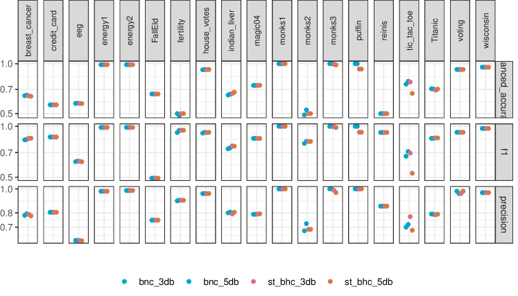
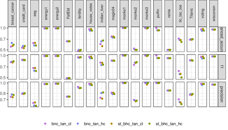
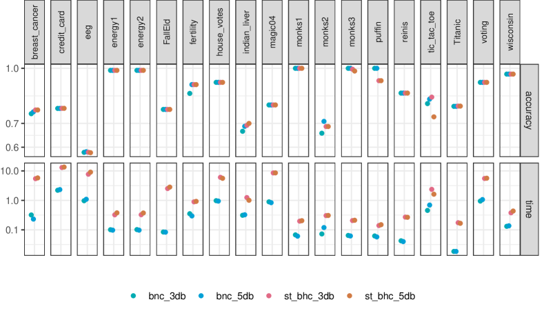
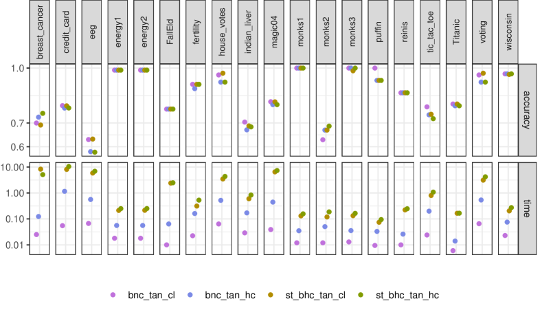
We compare the considered classifiers across various benchmark datasets, similarly to Carli et al. (2023) but also including some additional datasets with a larger number of features. Details about the datasets are given in Table LABEL:table:data, which also includes the normalized entropy of the class variable as a measure of dataset imbalance. For each dataset, we repeat 10 times an 80% - 20% train-test split and we report (Figures 16, 17, 18) median accuracies and elapsed times. Median F1 scores, balanced accuracies and precisions are reported in Appendix B.
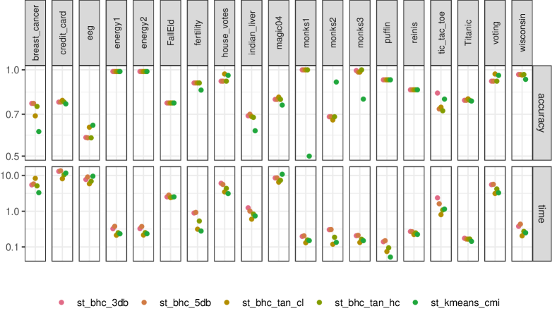
In Figure 16 we compare all considered staged tree classifiers. While TAN and -DB classifiers have comparable accuracy across all datasets, the naive staged tree is more variable, in some cases outperforming the others and in others having lower accuracy. All staged tree classifiers require a similar training time. In Figure 17 we compare staged trees -DB classifiers with their corresponding -DB BNCs and in Figure 18 we similarly compare TAN staged trees with corresponding TAN BNCs. It can be observed that overall the accuracy of all approaches is similar. In some instances BNCs outperform staged tree refinements, while in others the reverse can be observed. Considering TAN classifiers only, the st_bhc_tan_cl often outperform the others. As expected, staged tree refinements require more training time, but can still be learned in short time frames.
6.2 Simulations
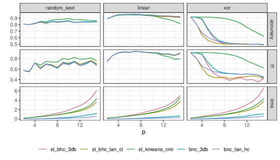
We perform a simulation study to explore how the classifiers behave under different scenarios. We consider three different data-generating processes:
-
•
random_sevt: generates a random staged tree model over binary variables, with the ordering and then samples from its induced joint distribution. Random staged trees are generated with the random_sevt function in the stagedtrees package. The function randomly joins stages starting from the full staged tree and assigns random conditional probabilities uniformly from the probability simplex.
-
•
linear: samples independent binary predictors as where . The class variable is then obtained as , where and .
-
•
xor: similar to the linear case, but with .
We vary the number of predictors () ranging from 2 to 15. For each case, we generate repetitions of training and test samples generated with the above three processes. In Figure 19 we report median accuracies, F1 scores and elapsed times across repetitions. The naive staged tree outperforms all other approaches for all values of under the random_sevt and xor simulation scenarios, while it has a decrease of performance in the linear data-generating scenario for large values of . The other algorithms have comparable performance except for the xor data generating scenario. The results in the xor scenario are partially to be expected: TAN and kDB BNC, as well as the staged tree refinements, cannot represent complex functions (Varando et al., 2015), and thus, as the number of predictors increases, their performance decrease drastically. As partially anticipated in Carli et al. (2023), the naive staged tree classifiers, here implemented with k-means clustering, can estimate optimal decision functions across a diverse range of data-generating processes, while only slightly worsening the sample-efficiency for larger .
7 Discussion
The paper introduced novel learning routines for subclasses of staged tree classifiers, which enhance BNCs with context-specific patterns of dependence. Experimental studies showed that in some scenarios they can outperform BNCs, although the difference in accuracy appears to be only marginal.
As with BNCs, different and specific parameter estimation techniques could be envisioned, such as discriminative learning (e.g. Pernkopf et al., 2011) and weighted schemes (e.g. Frank et al., 2002). Furthermore, adjusted class prior probabilities could be used to address imbalanced datasets, when different classification errors entail distinct costs (Wong and Tsai, 2021).
The simulation study suggests that naive staged tree classifiers are highly expressive, with high accuracy in the xor data generating scenario, where all other classifiers perform poorly. This fact led us to believe that naive staged trees may be able to theoretically represent any decision rule, or at least a set of decision rules much larger than those expressible by subclasses of BNCs. A formalization of this statement and its associated proof is currently being developed.
References
- Bielza and Larrañaga (2014) C. Bielza and P. Larrañaga. Discrete Bayesian network classifiers: A survey. ACM Computing Surveys, 47(1):1–43, 2014.
- Boutilier et al. (1996) C. Boutilier, N. Friedman, M. Goldszmidt, and D. Koller. Context-specific independence in Bayesian networks. In Proceedings of the Twelfth International Conference on Uncertainty in Artificial Intelligence, pages 115–123, 1996.
- Carli et al. (2022) F. Carli, M. Leonelli, E. Riccomagno, and G. Varando. The R package stagedtrees for structural learning of stratified staged trees. Journal of Statistical Software, 102:1–30, 2022.
- Carli et al. (2023) F. Carli, M. Leonelli, and G. Varando. A new class of generative classifiers based on staged tree models. Knowledge-Based Systems, 268:110488, 2023.
- Collazo et al. (2018) R. A. Collazo, C. Görgen, and J. Q. Smith. Chain event graphs. CRC Press, 2018.
- Devroye et al. (2013) L. Devroye, L. Györfi, and G. Lugosi. A probabilistic theory of pattern recognition. Springer Science & Business Media, 2013.
- Eggeling et al. (2019) R. Eggeling, I. Grosse, and M. Koivisto. Algorithms for learning parsimonious context trees. Machine Learning, 108:879–911, 2019.
- Frank et al. (2002) E. Frank, M. Hall, and B. Pfahringer. Locally weighted naive Bayes. In Proceedings of the 19th Conference on Uncertainty in Artificial Intelligence, pages 249–256, 2002.
- Freeman and Smith (2011) G. Freeman and J. Q. Smith. Bayesian MAP model selection of chain event graphs. Journal of Multivariate Analysis, 102(7):1152–1165, 2011.
- Friedman et al. (1997) N. Friedman, D. Geiger, and M. Goldszmidt. Bayesian network classifiers. Machine Learning, 29:131–163, 1997.
- Geiger and Heckerman (1996) D. Geiger and D. Heckerman. Knowledge representation and inference in similarity networks and Bayesian multinets. Artificial Intelligence, 82(1-2):45–74, 1996.
- Görgen et al. (2022) C. Görgen, M. Leonelli, and O. Marigliano. The curved exponential family of a staged tree. Electronic Journal of Statistics, 16(1):2607–2620, 2022.
- Hruschka Jr and Ebecken (2007) E. R. Hruschka Jr and N. F. Ebecken. Towards efficient variables ordering for Bayesian networks classifier. Data & Knowledge Engineering, 63(2):258–269, 2007.
- Keogh and Pazzani (2002) E. J. Keogh and M. J. Pazzani. Learning the structure of augmented Bayesian classifiers. International Journal on Artificial Intelligence Tools, 11(04):587–601, 2002.
- Leonelli and Varando (2022) M. Leonelli and G. Varando. Highly efficient structural learning of sparse staged trees. In International Conference on Probabilistic Graphical Models, pages 193–204. PMLR, 2022.
- Leonelli and Varando (2023) M. Leonelli and G. Varando. Context-specific causal discovery for categorical data using staged trees. In International Conference on Artificial Intelligence and Statistics, pages 8871–8888. PMLR, 2023.
- Leonelli and Varando (2024a) M. Leonelli and G. Varando. Learning and interpreting asymmetry-labeled DAGs: A case study on COVID-19 fear. Applied Intelligence, 54(2):1734–1750, 2024a.
- Leonelli and Varando (2024b) M. Leonelli and G. Varando. Robust learning of staged tree models: Ac case study in evaluating transport services. arXiv preprint arXiv:2401.01812, 2024b.
- Leonelli and Varando (2024c) M. Leonelli and G. Varando. Structural learning of simple staged trees. Data Mining and Knowledge Discovery, pages 1–25, 2024c.
- Minsky (1961) M. Minsky. Steps toward artificial intelligence. Transactions of the Institute of Radio Engineers, 49:8–30, 1961.
- Pernkopf et al. (2011) F. Pernkopf, M. Wohlmayr, and S. Tschiatschek. Maximum margin Bayesian network classifiers. IEEE Transactions on Pattern Analysis and Machine Intelligence, 34(3):521–532, 2011.
- Rios et al. (2024) F. L. Rios, A. Markham, and L. Solus. Scalable structure learning for sparse context-specific causal systems. arXiv preprint arXiv:2402.07762, 2024.
- Sahami (1996) M. Sahami. Learning limited dependence Bayesian classifiers. In Proceedings of the Second International Conference on Knowledge Discovery and Data Mining, pages 335–338, 1996.
- Scutari (2010) M. Scutari. Learning Bayesian networks with the bnlearn R package. Journal of Statistical Software, 35:1–22, 2010.
- Smith and Anderson (2008) J. Q. Smith and P. E. Anderson. Conditional independence and chain event graphs. Artificial Intelligence, 172(1):42–68, 2008.
- Varando et al. (2015) G. Varando, C. Bielza, and P. Larrañaga. Decision boundary for discrete Bayesian network classifiers. Journal of Machine Learning Research, 16:2725–2749, 2015.
- Varando et al. (2024) G. Varando, F. Carli, and M. Leonelli. Staged trees and asymmetry-labeled DAGs. Metrika, pages 1–28, 2024.
- Wong and Tsai (2021) T.-T. Wong and H.-C. Tsai. Multinomial naïve Bayesian classifier with generalized Dirichlet priors for high-dimensional imbalanced data. Knowledge-Based Systems, 228:107288, 2021.
Appendix A Benchmark Datasets Details
table:data Dataset # observations # variables # atomic events imbalance measure breast_cancer 277 10 332640 0.872 credit_card 30000 12 18432 0.762 eeg 14979 15 32768 0.992 energy1 768 9 1728 1.000 energy2 768 9 1728 1.000 fallEld 5000 4 64 0.888 fertility 100 10 15552 0.529 house_votes 232 17 131072 0.997 indian_liver 579 11 15552 0.862 magic04 19020 11 118098 0.936 monks1 432 7 864 1.000 monks2 432 7 864 0.914 monks3 432 7 864 0.998 puffin 69 6 768 0.999 reinis 1841 6 64 0.587 ticTacToe 958 10 39366 0.931 titanic 2201 4 32 0.908 voting 435 17 131072 0.997 wisconsin 683 10 1024 0.934
Appendix B Additional Results