FedSAC: Dynamic Submodel Allocation for Collaborative Fairness
in Federated Learning

Abstract.

Collaborative fairness stands as an essential element in federated learning to encourage client participation by equitably distributing rewards based on individual contributions. Existing methods primarily focus on adjusting gradient allocations among clients to achieve collaborative fairness. However, they frequently overlook crucial factors such as maintaining consistency across local models and catering to the diverse requirements of high-contributing clients. This oversight inevitably decreases both fairness and model accuracy in practice. To address these issues, we propose FedSAC, a novel Federated learning framework with dynamic Submodel Allocation for Collaborative fairness, backed by a theoretical convergence guarantee. First, we present the concept of ”bounded collaborative fairness (BCF)”, which ensures fairness by tailoring rewards to individual clients based on their contributions. Second, to implement the BCF, we design a submodel allocation module with a theoretical guarantee of fairness. This module incentivizes high-contributing clients with high-performance submodels containing a diverse range of crucial neurons, thereby preserving consistency across local models. Third, we further develop a dynamic aggregation module to adaptively aggregate submodels, ensuring the equitable treatment of low-frequency neurons and consequently enhancing overall model accuracy. Extensive experiments conducted on three public benchmarks demonstrate that FedSAC outperforms all baseline methods in both fairness and model accuracy. We see this work as a significant step towards incentivizing broader client participation in federated learning. The source code is available at https://github.com/wangzihuixmu/FedSAC.

1. Introduction

Federated Learning (FL) empowers multiple data owners to collectively train a global model while preserving the privacy of their individual training data (Xu et al., 2023; McMahan et al., 2017; Yan et al., 2023). Early FL frameworks (Li et al., 2020; Tan et al., 2023; Chen et al., 2023) usually distributed the same model to all clients without considering their distinct contributions to the model performance, resulting in unfairness to high-contributing clients. Collaborative fairness (CF) (Lyu et al., 2020b) stands as an essential element in federated learning to motivate client engagement by ensuring impartial reward distribution tied directly to individual contributions.

More recently, several gradient-based methods were proposed to enhance CF (Lyu et al., 2020b; Xu and Lyu, 2020; Xu et al., 2021; Wang et al., 2024) (i.e., rewarding clients with corresponding model quality according to their contributions) in FL. They distribute a larger quantity of gradients to higher-contributing clients than the lower ones as rewards and quantify the degree of fairness by Pearson Correlation Coefficient $\rho$. However, for achieving CF, existing gradient-based methods have  two major limitations. On one hand, the conventional definition of CF doesn’t adequately distinguish in reward distribution among clients, resulting in a persistent unfairness for high-contributing clients. In Figure 1 (a), suppose the contributions of three clients are $c=[1,9,11]$, and their rewards are $\theta^{*}=[99,99.2,99.3]$ corresponding. Through the definition of CF by CGSV (Xu et al., 2021), the fairness is calculated as $\gamma$=98.97, but there exists an underlying unfairness towards $Client_{2}$ and $Client_{3}$ because $Client_{1}$ with an inferior contribution is over-rewarded.  On the other hand, conventional gradient-based methods (Lyu et al., 2020b; Xu and Lyu, 2020; Xu et al., 2021; Wang et al., 2024) are ineffective because the inconsistency of local models updated by variable gradients might lead to significant degradation of overall model performance. In Figure 1 (a), the local models of clients in round $t$ ($\theta_{1,t}$, $\theta_{2,t}$, and $\theta_{3,t}$) exhibit notable differences (i.e., the larger the circle, the higher the accuracy). Consequently, the gradients uploaded by individual clients may not be the optimal for others, creating a misalignment between obtained rewards $\Delta_{\theta_{i,t}^{reward}}$ (i.e., the rewards ultimately obtained by the clients) and expected rewards $\Delta_{\theta_{i,t}^{exceppt}}$ (i.e., the rewards that the clients ultimately expected) for each client.

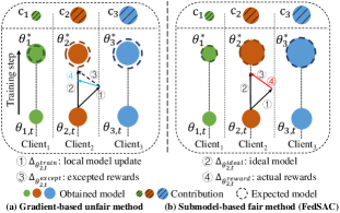
Figure 1. Problem illustration of collaborative fairness in FL. (a) Conventional gradients-based methods will result in poor fairness and model accuracy. For example, it is unfair that obtained models of $Client_{2}$ and $Client_{1}$ are equivalent neglecting the inferior contribution ($c_{1}$) of $Client_{1}$. Plus, the inconsistency in local models results in that obtained models of $Client_{2}$ and $Client_{3}$ are worse than expected ($\theta_{i}^{*}$). (b) Our proposed FedSAC allocates sufficient submodels to each client by ensuring a comprehensive balance between fairness and model accuracy. For example, FedSAC ensures that obtained models of all clients (i.e., $Client_{1}$, $Client_{2}$ and $Client_{3}$) are in accordance with their contributions respectively. In addition, FedSAC guarantees the alignment of ③ and ④ of $Client_{2}$ during the training process, thereby enabling all three clients to obtain their expected models ($\theta_{i}^{*}$).

To address the aforementioned challenges, we propose a novel Federated learning framework with dynamic Submodel Allocation for bounded Collaborative fairness (FedSAC), supported by a theory of convergence while achieving competitive model accuracy. First, our approach introduces the concept of ”bounded collaborative fairness (BCF) (refer to $Definition$ 1)”, which ensures fairness by integrating a differentiated range of rewards allocated to each client. Second, the submodel allocation module with a theoretical fairness guarantee, is designed to assign relevant submodels (i.e., results of the aggregated model dropout) to individual clients based on their contributions. Specifically, these submodels encompass a diverse array of essential neurons for effective training. Third, the dynamic aggregation module is implemented as a weight realignment mechanism by treating low-frequency neurons equally, which further improves the overall performance of the global model. Extensive experiments on three public benchmarks show that the proposed FedSAC outperforms all baseline methods in terms of collaborative fairness and model accuracy.

The contributions of this work are summarized:

• We propose FedSAC, a novel federated learning framework with a convergence guarantee, introducing a new concept of bounded collaborative fairness (BCF). To the best of our knowledge, this is the first approach that allocates submodels equitably for collaborative fairness in FL.

• We implement the concept of BCF through two modules. First, submodel allocation module prioritizes high-contributing clients by rewarding them with high-performance submodels under a theoretical guarantee. Second, dynamic aggregation module merges submodels by paying equitable attention to low-frequency neurons to be aggregated.

• We conduct extensive experiments on three benchmarks with various settings and demonstrate that FedSAC ourperforms all baselines in both fairness and model accuracy.

2. Related Works

Recent research has shown that distributing different rewards based on clients’ contributions can significantly impact the FL systems (Yang et al., 2019; Lyu et al., 2020a; Richardson et al., 2020). The incentive mechanisms can motivate clients to contribute high-quality data and promote collaboration (Xu et al., 2021; Shi et al., 2021; Khramtsova et al., 2020). We outline three types of rewards that can be adopted to achieve CF in FL.

Money-based reward. Several studies focus on the mechanism that rewards clients monetary based on their contributions. (Zhang et al., 2021) proposes a reputation-based and reverse auction theory mechanism to reward clients with a limited budget. (Yu et al., 2020) shows a scheme that dynamically allocates budgets to clients in a context-aware manner by jointly maximizing the collective utility. While monetary rewards can be a natural and effective way to incentivize clients in FL, there exist challenges in maintaining a balance between the value of model quality and money (Agarwal et al., 2019; Zhan et al., 2021).

Data-based reward. Early studies have explored the fairness of rewarding different data sizes based on their contributions.  (Sim et al., 2020) evaluates clients’ contributions by aggregating the training data, and reward them with the corresponding models. (Tay et al., 2022) trains a generative model through the local data of all clients and provides more synthetic data to those datasets closely aligned with the real data distribution. However, most of existing data-based reward methods rely on the centralized aggregation of all the data during training, making them difficult to be applied in the FL scenarios.

Gradient-based reward. Recent collaborative fairness (CF) works aim to reward high-contributing clients with optimal models. CFFL (Lyu et al., 2020b) allocates different gradient numbers based on local accuracy in the validation set and data sizes. CGSV (Xu et al., 2021) rewards more gradients to clients whose local gradients are more similar to the global gradients. FedAVE (Wang et al., 2024) assigns more gradients to clients whose data distribution information is more similar to the ideal dataset. However, existing rewards systems lack sufficient differentiation, resulting in an ongoing unfairness for high-contributing clients, which might degrade the fairness and model accuracy. Different from these methods, we propose a novel framework to achieve BCF (refer to $Definition$ 1) by allocating a differential range of rewards to clients.

3. Preliminary

FL system consists of a server and multiple clients, aiming to minimize the weighted average of all clients’ local objectives by optimizing a global model (McMahan et al., 2017; Huang et al., 2021; Zhang et al., 2023; Li et al., 2023). First, the server broadcasts a model to the clients at random. Second, after training several rounds locally, the server aggregates these different trained models into a new global model. Finally, the aggregated model will be sent to the clients for further local training. The aforementioned process is repeated multiple times until the global model converges (Mendieta et al., 2022; Gao et al., 2022a; Wang et al., 2023). In this setup, the goal of FL framework is defined as:

(1) $$\mathop{min}\limits_{\theta}F(\theta):=\sum\limits_{i=1}^{N}p_{i}F_{i}(\theta),$$

where $\theta$ denotes the global model, $N$ represents the number of clients, and $p_{i}=\frac{n_{i}}{n}$, $n=\sum_{k=1}^{N}n_{k}$. $F_{i}(\theta)$ is the loss on client $i$ using model parameters $\theta$, i.e., $F_{i}(\theta)=\frac{1}{n_{i}}\sum_{\xi_{i}\sim{D_{i}}}{l(\theta,\xi_{i})}$, where $D_{i}$ represents the local dataset of client $i$, and $n_{i}$ denotes the data size of $D_{i}$. To achieve this goal as effectively as possible, FedAvg (McMahan et al., 2017) samples a subset $S_{t}$ of $i$ clients uniformly, $0<i\leq N$, to train the global model and aggregate the locally trained models by utilizing the data size ratio $p_{i}$ as the weight of client $i$. Although FedAvg is proven to be effective in minimizing the objective successfully, it may be unfair to high-quality clients since the system distributes the same rewards to all clients regardless of their contributions (Lyu et al., 2020b; Xu et al., 2021).

3.1. Problem Formulation

The standard FL framework allocates the same model to all clients regardless of their contributions (McMahan et al., 2017; Sun et al., 2021; Huang et al., 2022; Qin et al., 2023), dampening the motivation of high-quality clients to join FL (Sim et al., 2020; Wang et al., 2020). Collaborative fairness in FL aims to reward high-contributing clients with high-quality models. The existing works (Lyu et al., 2020b; Xu et al., 2021; Wang et al., 2024) assess the fairness with the Pearson Correlation Coefficient, $\rho(c;\theta^{*})$, where $c$ and $\theta^{*}$ represent the contributions and rewards of clients, respectively. However, the definition simply considers the relationship between the contributions and rewards of clients, which may lead to insufficient incentives for high-contributing clients. For example in Figure 1 (a), suppose the contributions of $Client_{1}$, $Client_{2}$, and $Client_{3}$ are $c_{i}=[1,9,11]$ and their rewards are $\theta_{i}^{*}=[99,99.2,99.3]$ correspondingly. Through the definition of CF, the fairness is calculated as $\gamma$=98.97, but there exists an underlying unfairness towards $Client_{2}$ and $Client_{3}$ because $Client_{1}$ with an inferior contribution is over-rewarded.

To address this issue, we propose Bounded Collaborative Fairness (BCF) to tackle the issue of insufficient incentives for the high-contributing client. BCF could ensure $c_{1}<\theta_{1}^{*}<\frac{(c_{1}+\theta_{3}^{*})}{2}$ and then quantitative fairness with $\rho(c;\theta^{*})$. The rationale behind the formula in $Definition$ 1 aims to amplify significant distinctions in rewards. The formula’s left side ensures that clients’ rewards exceed their contributions, while the right side prevents excessive rewards for clients with low contributions.

Definition 0 (Bounded Collaborative Fairness).

The contributions ($c$) and the rewards ($\theta^{*}$) of clients are calculated by the performance of their standalone models (train without collaboration) and the final models obtained after collaboration, respectively. Based on client’s obtained rewards $c_{i}<\theta_{i}^{*}<\frac{(c_{i}+max(\theta^{*}))}{2}$, the quantitative fairness can be computed by $\gamma$ := 100 $\times$ $\rho$($c$, $\theta^{*}$) where $\rho$() is the Pearson Correlation Coefficient. The larger $\gamma$, the better the fairness of the framework.

4. The Proposed FedSAC

In this section, we will introduce the details of proposed FedSAC, a method that ensures both BCF and consistency in local models for each client. The architecture of FedSAC is shown in Figure 2. The pseudo codes for FedSAC are provided in Algorithm 1. First, we introduce the submodel allocation module in Section 4.1. Second, we present the dynamic aggregation module in Section 4.2. Third, we proposed the fairness guarantee theory in Section 4.3 to prove that this submodel allocation strategy can achieve collaborative fairness. Fourth, we conducted a convergence analysis on FedSAC and demonstrated its convergence in Section 4.5. In addition, we analyzed the time complexity and communication costs of FedSAC in Section 4.5. Finally, we discussed limitations in Section 4.6.

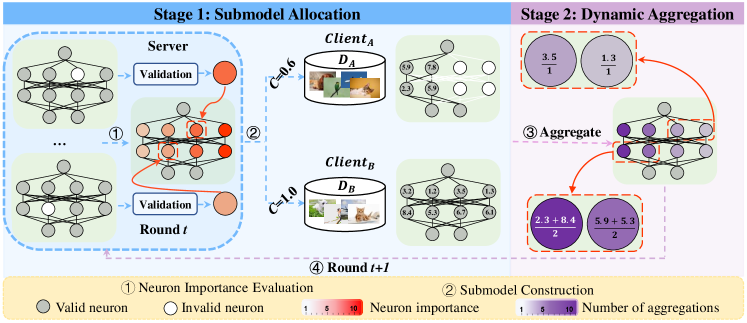
Figure 2.  The overall framework of FedSAC that achieves bounded collaborative fairness by maintaining consistency across local models. FedSAC consists of two module: 1)  submodel allocation module conducts neuron importance evaluation and submodel construction to reward high-contributing clients with high-performance submodels, thus ensuring consistency in local models; 2)  dynamic aggregation module treats those low-frequency neurons equally, which further refines the performance of the global model.

4.1. Submodel Allocation Module

A naive approach achieving bounded collaborative fairness involves allocating distinct submodels to each client based on their respective contributions (Hong et al., 2022). Unlike previous works such as (Horvath et al., 2021; Shi et al., 2023), there are two primary motivations behind achieving BCF through submodel allocation. First, submodels with appropriate pruning may not match the performance of the global model, enabling clients to receive diverse submodels according to their contributions. Second, despite being subsets of the global model, these submodels exhibit strong mutual validity, meaning that the submodels uploaded by one client are effective for others, facilitating the training of the global model. However, it is still challenging to achieve BCF through submodel-based methods. For one thing, it is crucial to ensure that the majority of neurons are adequately trained to guarantee the optimal performance of the global model. For another, the performance of allocated submodels should align with their respective contributions.

To address the aforementioned two challenges, we design a two-step approach for submodel allocation module. First, we evaluate the importance of each neuron within the model to determine their contributions respectively (neuron importance evaluation in Section 4.1.1). Second, we construct submodels for each client with varying performances based on their contributions, ensuring a diverse array of important neurons is included within each submodel (submodel construction in Section 4.1.2).

4.1.1. Neuron Importance Evaluation

Each neuron within the model holds a unique contribution (Luo et al., 2017; Molchanov et al., 2017; Yu et al., 2018; Molchanov et al., 2019). Our intuition is that the constructed submodels can yield varied performances. Inspired by Taylor-FO (Molchanov et al., 2019), we calculate the neuron importance in the model by measuring the change in loss upon their removal. For instance, a greater increase in loss indicates a more significant contribution by the removed neuron to the model. In Figure 2, neurons depicted in a redder shade represent a higher contribution to the model. Essentially, the training objective is to minimize the cross-entropy loss $L_{ce}$:

(2) $$\min\limits_{\theta}\sum\limits_{i=1}^{N}L_{ce}(x_{i},\theta),$$

where $x_{i}$ denotes the sample, $\theta$ represents the model, and $L_{ce}(x_{i},\theta)$ is the loss function of the classification tasks.

The neurons in the model have a multitude of model parameters, each of which contributes to the overall performance of the model. The importance of a neuron $I_{n_{i}}$ of the model can be calculated through the loss increased by removing it:

(3) $$I_{n_{i}}=L_{ce}(V,\theta|\theta_{n_{i}}^{zero}=0)-L_{ce}(V,\theta),$$

where $V$ denotes the validation set, which is constructed by evenly selecting 10% of the data from the original training samples (Lyu et al., 2020b), $\theta_{n_{i}}^{zero}$ represents that the parameters of the $i$-th neuron in the model are all set to 0.

To simplify the construction of submodels, we normalize the sum of neuron scores, which represent their importance in the model presented by percentage:

(4) $$I_{n_{i}}=\frac{I_{n_{i}}}{\sum\nolimits_{n_{i}\in{S}}I_{n_{i}}}*100,$$

where $S$ represents all neurons of the model. To reduce the training time of the framework, we measure the importance of neurons in the model by Eq. (3) and Eq. (4) every 10 epochs. All these operations allow us to efficiently assess the importance of each neuron while limiting excessive computation demands.

4.1.2. Submodel Construction

In pursuit of fairness, we employ a dynamic allocation system for submodels with varying performances, leveraging clients’ reputations derived from their contributions. Our approach incorporates a pruning mechanism tailored to clients’ contributions, simplifying the extraction of submodels with different performance levels from the global model. In this scheme, the client $i$’s reputation $r_{i}$ is expressed as:

(5) $$r_{i}=e^{{c_{i}}*\beta},$$

(6) $$r_{i}=\frac{r_{i}}{max(r)}*100,$$

where $c_{i}$ represents client $i$’s contribution, $\beta$ is a hyper-parameter. The reputations of clients are directly proportional to their contributions. The design rationale for Eq. (5) and Eq. (6) is to calculate the clients’ reputations ($r$), which facilitates the allocation of their submodels fairly. More specifically, our pruning method begins with the most important neuron, ensuring that submodels for low-contribution clients possess a higher parameter count, which is beneficial for training the global model. These actions serve a dual purpose: promoting collaborative fairness while maximizing the overall performance of the global model. Submodel $\theta_{i}$ is constructed by neurons with different reputations:

(7) $$\theta_{i}=quantity(r_{i},\sum\nolimits_{n_{i}\in{S}}I_{n_{i}}),$$

where $quantity(r_{i},\sum\nolimits_{n_{i}\in{S}}I_{n_{i}})$ represents the submodel $\theta_{i}$ when $r_{i}=\sum\nolimits_{n_{i}\in{S}}I_{n_{i}}$, $r_{i}$ denotes client $i$’s reputation, $\sum\nolimits_{n_{i}\in{S}}I_{n_{i}}$ denotes the set importance for different neurons. $S$ represents the positions of all neurons in the model, arranged in ascending order from the least to the most important. This design choice aims to maximize the inclusion of neurons in each submodel, thereby enhancing the performance of the corresponding local model updates. Subsequently, this quantity will be utilized in Eq. (8) to generate the submodel’s mask.

4.2. Dynamic Aggregation Module

Next, the server aggregates the locally trained submodels and allocates distinct submodels to clients in the subsequent round. Recent submodel-based methods (Horvath et al., 2021; Shi et al., 2023) have aimed to allocate varied submodels containing numerous neurons to clients. However, these approaches might pose a potential risk of compromising overall model performance when integrating low-frequency neurons into the global model. Consequently, employing a direct aggregation method such as FedAvg (McMahan et al., 2017) for all neurons becomes inequitable.

Instead of simply averaging the uploaded submodels, our objective is to optimize the utilization of all neurons within the model. With the sizes of submodels varying across clients, it becomes essential to treat the contribution of each neuron individually during aggregation. To ensure fair treatment of low-frequency neurons, we integrate the frequency of submodel parameter aggregations as weights to dynamically aggregating local models:

(8) $$mask_{i}^{t}=mask(\theta_{i}^{t},\theta_{g}^{t-1}),$$

(9) $$\theta_{g}^{t+1}=\frac{\sum\nolimits_{i\in{N}}\theta_{i}^{t}}{\sum\nolimits_{i\in{N}}mask_{i}^{t}},$$

where $mask(\theta_{i},\theta_{g})$ denotes submodel $\theta_{i}$’s mask (same shape as the submodel $\theta_{i}$), $\theta_{g}$ denotes the aggregated model, $N$ denotes the total number of clients. It sets the components of both $\theta_{i}$ and $\theta_{g}$ at the same position to 1 and 0 for the rest. The role of the mask function $mask(\theta_{i},\theta_{g})$ is to calculate the frequency of each model parameter $\theta_{i}$ selected by the global model $\theta_{g}$ in round $t$. Later, the mask function $mask(\theta_{i},\theta_{g})$ will be utilized in Eq. (9) to treat those low-frequency parameters equally by suppressing the weight of high-frequency parameters in the aggregation, which makes each parameter play a fair role during the aggregation phase. For example, the more the frequency of a selected parameter in round $t$, the smaller the weight of the parameter to be aggregated in round $t+1$.

4.3. Fairness Guarantee

In Section 4.1, we delved into the fundamental concept underpinning our definition of fairness. This concept centers on rewarding high-contributing clients with high-performance submodels, where a submodel’s improved performance correlates with the number of neurons it contains. Consequently, this approach leads to a training loss (i.e., model accuracy) that more closely aligns with the aggregated model. It’s important to note that the submodel $\theta_{i}$ acquired by client $i$ is determined based on its reputation $r_{i}$ across the entire training process up to iteration $t$.

Our primary result ensures a notion of fairness under specific conditions concerning the loss function $F$. If client $i$ holds a higher reputation than client $j$ ($r_{i}\geq r_{j}$), and the submodel $\theta_{i}^{t}$ obtained by client $i$ encompasses the submodel $\theta_{j}^{t}$ obtained by client $j$ ($\theta_{j}^{t}\in\theta_{i}^{t}\in\theta_{g}^{t}$). Then, the submodel $\theta_{i}^{t}$ obtained by client $i$ will exhibit closer alignment with the aggregated model $\theta_{g}^{t}$ in round $t$. Letting $\delta_{i}^{t}:=||\theta_{g}^{t}-\theta_{i}^{t}||$, it’s evident that $\delta_{i}^{t}\leqslant\delta_{j}^{t}$. Consequently, the submodel $\theta_{i}^{t}$ obtained by client $i$ will yield a smaller loss function $F(\theta)$ compared to client $j$ in round $t$.

Assumption 1 ($L$-smooth F).

If $F$ is $L$-smooth, then ${\forall}\theta_{i},\theta_{j}\in\theta$,

(10) $$F(\theta_{i})\leqslant F(\theta_{j})+\nabla F(\theta_{j})^{T}(\theta_{i}-\theta_{j})+\frac{L}{2}||\theta_{i}-\theta_{j}||^{2}.$$

Assumption 2 ($\mu$-strongly convex F).

If $F$ is $\mu$-strongly convex, then ${\forall}\theta_{i},\theta_{j}\in\theta$,

(11) $$F(\theta_{i})\geq F(\theta_{j})+\nabla F(\theta_{j})^{T}(\theta_{i}-\theta_{j})+\frac{\mu}{2}||\theta_{i}-\theta_{j}||^{2}.$$

Theorem 1 (Fairness in Training Loss).

Assume Assumptions 1 and 2 hold, FedSAC can guarantee collaborative fairness by rewarding high-contributing clients obtaining high-performance models. Formally speaking, let $\delta_{i}^{t}:=||\theta_{g}^{t}-\theta_{i}^{t}||$. Suppose that $\theta_{t}$ is close to a stationary point of $F$ for $t\geq T\in Z^{+}$, and $F()$ is both $L$-smooth and $\mu$-strongly convex with $L\leqslant\mu$. For all $i,j\in N$ in round t, if $r_{i}\geq r_{j}$, it follows that $\theta_{j}^{t}\in\theta_{i}^{t}\in\theta_{g}^{t}$, $\delta_{i}^{t}\leqslant\delta_{j}^{t}$, and therefore $F(\theta_{i}^{t})\leqslant F(\theta_{j}^{t})$.

The proof process is as follows:

From $L$-smoothness (ASSUMPTION 10), we have

(12) $$F(\theta_{i}^{t})\leqslant\underbrace{F(\theta_{N}^{t})+\nabla F(\theta_{N}^{t})^{T}(\theta_{i}^{t}-\theta_{N}^{t})+\frac{L}{2}\delta_{i,t}^{2}}_{\text{$R_{L}$}}.$$

From $\mu$-strongly convex (ASSUMPTION 11), we have

(13) $$F(\theta_{j}^{t})\geq\underbrace{F(\theta_{N}^{t})+\nabla F(\theta_{N}^{t})^{T}(\theta_{j}^{t}-\theta_{N}^{t})+\frac{\mu}{2}\delta_{j,t}^{2}}_{\text{$R_{\mu}$}}.$$

In order to prove $F(\theta_{i}^{t})\leqslant F(\theta_{j}^{t})$, it suffices to prove $R_{L}\leqslant R_{\mu}$ or equivalently $R_{L}-R_{\mu}\leqslant 0$.

(14) $$R_{L}-R_{\mu}=\underbrace{\nabla F(\theta_{N}^{t})^{T}(\theta_{i}^{t}-\theta_{j}^{t})}_{\text{$R_{1}$}}+\underbrace{\frac{1}{2}(L\delta_{i,t}^{2}-\mu\delta_{j,t}^{2})}_{\text{$R_{2}$}}.$$

With $L\leqslant\mu$ and $\delta_{i,t}\leqslant\delta_{j,t}$, we have

(15) $$R_{2}=\frac{1}{2}(L\delta_{i,t}^{2}-\mu\delta_{j,t}^{2})\leqslant\frac{L}{2}(\delta_{i,t}^{2}-\delta_{j,t}^{2})\leqslant 0.$$

We define $\theta_{N}^{t}$ being close to a stationary point of F by establishing an upper limit on the gradient:

(16) $$||\nabla F(\theta_{N}^{t})||\leqslant\frac{L|\delta_{i,t}^{2}-\delta_{j,t}^{2}|}{2||\theta_{i}^{t}-\theta_{j}^{t}||}.$$

We have the following:

(17) $$\begin{split}|R_{1}|&\triangleq|\nabla F(\theta_{N}^{t})^{T}(\theta_{i}^{t}-\theta_{j}^{t})|\\ &\leqslant||\nabla F(\theta_{N}^{t})||\times||(\theta_{i}^{t}-\theta_{j}^{t})||\\ &\leqslant\frac{L|\delta_{i,t}^{2}-\delta_{j,t}^{2}|}{2}\\ &\leqslant|R_{2}|,\end{split}$$

where the first inequality is derived from the Cauchy-Schwarz, the second inequality is by substituting the aforementioned upper limit (refer to Eq. (16)), and the last inequality (line 1209) emerges from taking the absolute values of two negative values (refer to Eq. (15)).

Finally, given that $|R_{1}|\leqslant|R_{2}|$ and $R_{2}\leqslant 0$, we derive $R_{1}+R_{2}\leqslant 0$. Therefore, it follows that $R_{L}-R_{\mu}\triangleq R_{1}+R_{2}\leqslant 0$, which subsequently implies $F(\theta_{i}^{t})\leqslant F(\theta_{j}^{t})$.

Algorithm 1 FedSAC

1:The global model $\theta_{g}$, the local submodel $\theta_{i}$, neurons $i$’s importance $I_{n_{i}}$, the number of local update steps $E$, learning rate $\eta_{t}$, number of clients $N$, hyper-parameter $\beta$, client’s contribution $c$

2:Initialize the global model parameters $\theta_{g}^{0}$

3:for round $t=0,1,...,T-1$ do

4:     Compute $I_{n_{i}}^{t}$ (3) and (4) of $\theta_{g}^{t}$

5:     Calculate the reputation $r_{i}$ of client $k$: $r_{i}=\frac{e^{{c_{i}}*\beta}}{max(e^{{c}*\beta})}*100$

6:     Calculate Submodels $\theta_{i}^{t}$ of clients $i$ in round $t$: $\theta_{i}^{t}=quantity(r_{i},\sum\nolimits_{n_{i}\in{S}}I_{n_{i}}^{t})$

7:     for each client $i\in{N}$ do

8:         for each iteration $j=0,1,...,E-1$ do

9:              $\theta_{i,j+1}^{t}\leftarrow{\theta_{i,j}^{t}}-$ $\eta_{t}\nabla{F_{i}(\theta_{i,j}^{t})}$

10:         end for

11:     end for

12:     Submodel $i$’s mask in round $t$: $mask_{i}^{t}=mask(\theta_{i}^{t},\theta_{g}^{t-1})$

13:     The server aggregates the received submodels: $\theta_{g}^{t+1}=\frac{\sum\nolimits_{i\in{N}}\theta_{i}^{t}}{\sum\nolimits_{i\in{N}}mask_{i}^{t}}$

14:end for

4.4. Convergence Analysis

In this section, we delve into the convergence analysis of the proposed FedSAC. To guarantee convergence to the global optimum, we make the assumption that each neuron in the aggregated model is equally allocated over $T$ rounds. Consequently, the anticipated weight of the allocated submodel $\theta_{i}$ contracts towards the aggregate model $\theta_{g}$, i.e., $\theta_{i}^{t+1}=p_{i}\theta_{g}^{t}$. Here, $p_{i}$ ($0\leqslant p_{i}\leqslant 1$) denotes the long-term expectation of the size ratio between the submodel $i$ and the aggregate model obtained in multiple iterations. At this stage, Eq. (9) can be expressed as the aggregation of each submodel $\theta_{i}$ divided by its respective $p_{i}$, i.e., $\theta_{g}^{t+1}=\sum_{i=1}^{N}\frac{\theta_{i}^{t+1}}{p_{i}}$. We present THEOREM 2 below, which demonstrates that FedSAC enables the convergence of the aggregation model. Assumptions 3 and 4 are derived from the works (Zhang et al., 2012; Stich, 2018; Stich et al., 2018; Yu et al., 2019).

Assumption 3.

Let $\xi_{i}^{t}$ denote samples uniformly from the local data of the $i$-th device at random. It is asserted that the variance of stochastic gradients within each device remains constrained:

(18) $$E\|\nabla F_{i}(\theta_{i}^{t},\xi_{i}^{t})-\nabla F_{i}(\theta_{i}^{t})\|\leqslant\sigma_{i}^{2},$$

Assumption 4.

The expected squared norm of stochastic gradients is uniformly constrained:

(19) $$E\|\nabla F_{i}(\theta_{i}^{t},\xi_{i}^{t})\|\leqslant G^{2},$$

where $i\in\{1,2,...,$N$\}$ and $t\in\{1,2,...,T-1\}$.

Assumption 5.

Each neuron in the aggregation model is assigned the same number of times after $T$ rounds. Therefore, the expected weight of the allocated submodel $\theta_{i}$ is a contraction of the aggregate model $\theta_{g}$, i.e., $\theta_{i}^{t+1}=p_{i}\theta_{g}^{t}$. Here, $p_{i}$ ($0\leqslant p_{i}\leqslant 1$) denotes the long-term expectation of the size ratio between the submodel $i$ and the aggregate model obtained in multiple iterations.

Theorem 2 (Asymptotic convergence).

Given that Assumptions 10 to 5 hold and $L$, $\mu$, $\sigma_{i}$, $G$, $p$ be defined therein. Choose $\kappa=\frac{2}{\mu}$, $\gamma=max\{8\frac{L}{\mu},E\}-1$ and the learning rate $\eta_{t}=\frac{2}{\mu(\gamma+t)}$. Then FedSAC satisfies $E[F(\bar{\theta}_{T})]-F^{*}\leqslant[\frac{L}{\gamma+T}(\frac{2B}{\mu^{2}}+\frac{\gamma+1}{2}\triangle_{1})]$.

The proof is shown in Appendix A.

4.5. Complexity and Communication Cost Analysis

We further analyze the time complexity and communication costs of FedSAC as follows.

For the time complexity, the primary computational demand in FedSAC stems from evaluating neuron importance, as defined in Eq. (3) and Eq. (4)). The time complexity for this evaluation is $O(M)$, where $M$ denotes the total number of neurons across the hidden layers of the global model.

For the communication cost, FedSAC mitigates the introduction of additional communication overhead by conducting neuron importance evaluation solely on the server. This approach effectively eliminates the necessity for client-server communication, thereby enhancing overall efficiency. Moreover, it displays a communication complexity of O(d*m) per round, as outlined in (Horvath et al., 2021), where m$\leqslant$1 denotes the average ratio of submodel parameters to the global model. As a result, FedSAC showcases lower communication complexity compared to all baseline methods in cross-silo FL scenarios (Ogier du Terrail et al., 2022). More details about the communication cost experiments are put in Appendix E.

4.6. Limitations

In Table 1 and Table 2, we conduct extensive experiments on various datasets and observe that FedSAC could exhibit a distinct advantage over all baseline methods in terms of both fairness and model accuracy. Nevertheless, the sufficient evaluation of neuron importance (Section 4.1.1) within the submodel allocation module imposes an additional computational burden. This problem may be amplified for large models. Despite this challenge, we hold a strong conviction that the substantial enhancements in both fairness and accuracy achieved through by FedSAC clearly affirm its superiority over baseline methods.

5. Experiments

In this section, we conduct comprehensive experiments to answer the following research questions:

RQ1. How does the fairness of our FedSAC compare to various state-of-the-art methods?

RQ2. How does the predictive model performance achieved by our proposed method compare with the state-of-the-art methods on different datasets?

RQ3. How do different components (i.e., submodel allocation module and dynamic aggregation module) affect the results?

5.1. Experimental Settings

Datasets and Models. We evaluate the performance of FedSAC on three commonly used public datasets in collaborative fairness, including Fashion MNIST (LeCun et al., 1998), CIFAR10 (Krizhevsky et al., 2009), and SVHN (Netzer et al., 2011). Following (Lin et al., 2020; Li et al., 2021; Uddin et al., 2020), we employ a feedforward neural network with two hidden layers for all datasets.

Data splits. We construct five heterogeneous scenarios by varying the size and the class numbers of the dataset. For imbalanced dataset sizes (POW) (Lyu et al., 2020b; Xu et al., 2021), we randomly divide the total dataset into various data sizes for each client by using a power law. For CIFAR10, we partition the data set of size 20000 among 10 clients. The clients with more extensive data sizes are expected to achieve better prediction performance. For imbalanced class numbers (CLA)  (Lyu et al., 2020b; Xu et al., 2021), we change the number of classes and keep them have the same amount of data. For CIFAR10 with 5 clients, clients 1, 2, 3, 4, 5 own local training data with 1, 3, 5, 7, 10 classes respectively. For imbalanced data size and class numbers (DIR), we provide clients with various data sizes and classes by the Dirichlet distribution function (Chen et al., 2022; Yurochkin et al., 2019; Gao et al., 2022b; Yu et al., 2022). Specifically, we sample $p_{i}^{l}\sim DIR(\alpha)$ and assign a $p_{i}^{l}$ percentage of the data of class $l$ to client $i$, where $DIR(\alpha)$ is the Dirichlet distribution with a parameter $\alpha$. More details on the varying numbers of clients used in the experiment are put in Appendix C.

Dataset	CIFAR10					SVHN					Fashion MNIST
No. Clients	10					10					10
Scene	POW	CLA	DIR(1.0)	DIR(2.0)	DIR(3.0)	POW	CLA	DIR(1.0)	DIR(2.0)	DIR(3.0)	POW	CLA	DIR(1.0)	DIR(2.0)	DIR(3.0)
FedAvg(McMahan et al., 2017)	14.55$\pm$25.4	84.68$\pm$3.5	10.77$\pm$6.3	15.06$\pm$21.2	68.93$\pm$8.1	-19.24$\pm$26.7	71.42$\pm$13.0	58.56$\pm$4.0	50.95$\pm$13.5	31.43$\pm$19.0	-19.83$\pm$24.1	78.44$\pm$4.3	17.94$\pm$7.3	60.36$\pm$16.3	76.09$\pm$29.5
q-FFL(Li et al., 2019b)	34.91$\pm$15.1	98.74$\pm$0.5	90.89$\pm$1.5	89.01$\pm$1.5	73.02$\pm$2.5	67.97$\pm$11.6	93.05$\pm$1.0	82.11$\pm$1.8	86.87$\pm$4.7	89.41$\pm$2.1	42.69$\pm$9.8	88.99$\pm$0.3	73.19$\pm$6.0	83.93$\pm$0.7	79.99$\pm$7.3
CFFL(Lyu et al., 2020b)	93.55$\pm$1.3	89.99$\pm$0.8	29.90$\pm$3.6	81.82$\pm$0.8	59.86$\pm$3.0	96.38$\pm$1.5	95.63$\pm$0.4	46.91$\pm$5.7	38.58$\pm$2.5	31.35$\pm$8.3	90.94$\pm$0.5	86.50$\pm$0.7	85.90$\pm$0.9	85.09$\pm$1.3	71.10$\pm$0.3
CGSV(Xu et al., 2021)	90.78$\pm$0.6	91.04$\pm$0.8	63.29$\pm$3.6	84.59$\pm$1.6	84.75$\pm$0.2	90.99$\pm$0.4	87.22$\pm$0.6	72.09$\pm$0.2	72.19$\pm$0.2	76.31$\pm$0.2	95.34$\pm$0.3	73.65$\pm$2.6	82.91$\pm$3.6	82.91$\pm$3.6	84.95$\pm$1.3
FedAVE(Wang et al., 2024)	85.50$\pm$0.8	92.80$\pm$1.2	58.43$\pm$0.9	85.82$\pm$0.7	88.61$\pm$1.3	92.68$\pm$0.4	92.77$\pm$0.8	82.42$\pm$1.2	64.83$\pm$1.0	79.38$\pm$0.8	86.98$\pm$0.5	86.36$\pm$1.1	79.51$\pm$1.3	87.99$\pm$0.5	67.62$\pm$0.3
Ours	98.80$\pm$0.2	99.06$\pm$0.3	99.14$\pm$0.6	95.73$\pm$0.5	97.01$\pm$0.7	99.44$\pm$0.3	99.74$\pm$0.1	96.09$\pm$0.3	96.48$\pm$0.2	98.32$\pm$0.8	96.35$\pm$0.2	98.93$\pm$0.7	99.23$\pm$0.3	97.71$\pm$0.2	98.62$\pm$0.3

Table 1.  Comparison results of fairness $\rho\in[-100,100]$ with state-of-the-art methods on three datasets. The reported results are averaged over 5 runs with different random seeds. (A higher value indicates better fairness. The best average result is marked in bold. The second-best result is underlined. These notes are the same to others.)

Dataset	CIFAR10					SVHN					Fashion MNIST
No. Clients	10					10					10
Scene	POW	CLA	DIR(1.0)	DIR(2.0)	DIR(3.0)	POW	CLA	DIR(1.0)	DIR(2.0)	DIR(3.0)	POW	CLA	DIR(1.0)	DIR(2.0)	DIR(3.0)
Standalone	41.23$\pm$0.1	37.49$\pm$0.2	33.78$\pm$0.2	33.54$\pm$0.1	31.89$\pm$0.1	60.02$\pm$0.2	52.05$\pm$0.3	41.41$\pm$0.2	58.07$\pm$0.2	61.11$\pm$0.2	84.36$\pm$0.2	82.52$\pm$0.3	64.19$\pm$0.3	67.39$\pm$0.1	74.29$\pm$0.2
FedAvg(McMahan et al., 2017)	48.36$\pm$0.2	42.64$\pm$0.5	48.84$\pm$0.1	49.49$\pm$0.5	49.72$\pm$0.5	74.16$\pm$0.2	68.25$\pm$0.1	77.75$\pm$0.2	78.17$\pm$0.1	81.35$\pm$0.1	87.64$\pm$0.2	85.42$\pm$0.0	87.32$\pm$0.1	87.27$\pm$0.2	88.25$\pm$0.2
q-FFL(Li et al., 2019b)	46.22$\pm$1.5	41.40$\pm$0.2	35.00$\pm$0.9	37.41$\pm$1.1	37.81$\pm$0.4	69.61$\pm$0.6	54.71$\pm$1.52	34.15$\pm$0.6	44.69$\pm$1.3	56.92$\pm$1.1	85.44$\pm$0.2	82.93$\pm$0.5	65.51$\pm$2.4	69.61$\pm$2.1	78.96$\pm$0.8
CFFL(Lyu et al., 2020b)	47.94$\pm$0.6	42.12$\pm$0.3	44.44$\pm$0.9	48.44$\pm$0.3	47.56$\pm$1.2	72.68$\pm$0.2	69.66$\pm$0.7	75.89$\pm$0.9	75.21$\pm$0.3	77.01$\pm$0.9	87.40$\pm$0.4	85.29$\pm$0.4	86.16$\pm$1.0	87.23$\pm$0.2	87.11$\pm$0.8
CGSV(Xu et al., 2021)	34.60$\pm$0.7	39.33$\pm$0.5	47.22$\pm$0.6	44.12$\pm$0.5	39.31$\pm$0.7	65.92$\pm$0.6	65.96$\pm$0.3	73.00$\pm$1.9	75.16$\pm$0.2	77.42$\pm$0.5	83.16$\pm$0.3	82.41$\pm$1.3	85.03$\pm$2.9	84.73$\pm$3.2	76.51$\pm$4.2
FedAVE(Wang et al., 2024)	46.51$\pm$0.2	35.18$\pm$1.5	46.60$\pm$0.6	39.20$\pm$1.2	40.60$\pm$1.8	70.80$\pm$0.5	65.10$\pm$0.6	73.44$\pm$0.6	73.43$\pm$0.3	75.48$\pm$0.7	86.18$\pm$0.6	79.86$\pm$1.2	76.66$\pm$0.8	80.90$\pm$1.3	67.74$\pm$0.8
Ours	48.61$\pm$0.2	44.16$\pm$0.2	49.06$\pm$0.6	50.01$\pm$0.2	49.85$\pm$0.3	74.84$\pm$0.2	70.51$\pm$0.8	78.06$\pm$0.1	78.55$\pm$0.1	81.95$\pm$0.4	87.88$\pm$0.2	85.61$\pm$0.3	87.85$\pm$0.1	87.54$\pm$0.4	88.38$\pm$0.4

Table 2.  Comparison results of the maximum test accuracy ($\%$) with state-of-the-art methods on three datasets. The reported results are averaged over 5 runs with different random seeds. (A higher value indicates better accuracy.)

Baselines. We compare FedSAC with the following methods: (1) FedAvg (McMahan et al., 2017) distributes the same model to all clients in each FL iteration. In this case, Pearson Correlation Coefficient $\rho()$ in Section 3.1 is uncomputable. To address this and create a personalized model for each client, we follow CFFL (Lyu et al., 2020b) and CGSV (Xu et al., 2021), which enables clients to train for an additional epoch at the end of FL algorithm. (2) q-FFL(Li et al., 2019b) enables the reweighting of loss across different clients by the q-parameterized weights, thus reducing the variance in the accuracy distribution and achieving a fairer distribution of accuracy. (3) CFFL (Lyu et al., 2020b) allocates more gradients to higher reputation client, and the reputation is calculated by the local accuracy and data sizes (or label diversity). (4) CGSV (Xu et al., 2021) assigns more gradients to clients whose local model gradients is more similar to the global gradients. (5) FedAVE (Wang et al., 2024) assigns more gradients to clients whose data distribution information is more similar to the ideal dataset. (6) Standalone (Lyu et al., 2020b) trains local models alone without collaboration. Particularly, to evaluate more fairly, we make all algorithms distribute rewards based on client contributions rather than the calculated reputations.

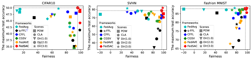
Figure 3.  Comparison results of overall performance to achieve bounded collaborative fairness with state-of-the-art methods in CIFAR10 (left), SVHN (middle), and Fashion MNIST (right). (The closer the point is to the upper-right corner, the better the performance.)

Hyper-Parameters. We tune all hyper-parameters in datasets by using grid search with FedAvg (McMahan et al., 2017) and subsequently apply the optimal parameters obtained from the validation dataset. The batch size is $B$ = 64 for SVHN and $B$ = 32 for both FashionMNIST and CIFAR10. The optimal parameters for SVHN, Cifar10, and FashionMNIST of six scenarios are $E$ = {15, 20}, $\eta$ = {0.05, 0.1}, $\beta$ = {3, 5, 10}; $E$ = {15, 20}, $\eta$ = {0.03, 0.05}, $\beta$ = {3, 5, 10}, and $E$ = 20, $\eta$ = {0.03, 0.05}, $\beta$ = {1, 10, 20, 25}, respectively. For comparison, we select the best fairness achieved by each method. The effects of hyper-parameter $\beta$ on FedSAC are detailed in Appendix D (the smaller $\beta$ is, the higher the accuracy achieved by FedSAC). More details about the hyper-parameters are put in Appendix F.

Implementation. All experiments are run on a 64 GB-RAM Ubuntu 18.04.6 server with Intel(R) Xeon(R) CPU E5-2630 v4 @ 2.20GHz and 1 NVidia(R) 2080Ti GPUs.

5.2. Experimental Results

Fairness (RQ1). To evaluate the FedSAC fairness, we compared it with a few baselines on three datasets. Table 1 shows the fairness metrics according to $Definition$ 1. Standalone (Lyu et al., 2020b) trains local models alone without collaboration, which represents the clients’ contributions. Table 1 indicates that our proposed dynamic submodel allocation mechanism achieves a fairness score above 95.73% on all datasets, while the FedAvg performs poorly with the lowest fairness score of -19.83%. On three datasets, the fairness of algorithms (i.e., CFFL, CGSV, and FedAVE) exceeds 73.65% for the POW and CLA scene. In these scenarios, the client’s contribution varies greatly and is mainly related to the amount of data or diverse labels of data. For the DIR scene, the data distribution among clients is significantly uneven, resulting in a high degree of non-iid settings and clients with relatively similar contributions. Consequently, CFFL, CGSV, and FedAVE show low fairness, as the rewards received by clients tend to be indistinguishable. In particular, in DIR (1.0) of CIFAR10, our method outperforms CFFL, CGSV and FedAVE by 69.24%, 35.85%, and 40.71%, respectively.

Table 1 demonstrates that the proposed FedSAC outperforms the state-of-the-art approaches in fairness, and validated the effectiveness of our method: high-contributing clients obtain high-performance models. Figure 3 shows the comparison results of overall performance to achieve bounded collaborative fairness with state-of-the-art methods in CIFAR10 (left), SVHN (middle), and Fashion MNIST (right). Obviously, FedSAC outperforms all baselines in terms of fairness.

Dataset	CIFAR10					SVHN					Fashion MNIST
Scene	POW	CLA	DIR(1.0)	DIR(2.0)	DIR(3.0)	POW	CLA	DIR(1.0)	DIR(2.0)	DIR(3.0)	POW	CLA	DIR(1.0)	DIR(2.0)	DIR(3.0)
$w/o$ $allocation$	79.99	96.47	10.93	43.81	-14.61	96.88	94.88	31.86	64.94	82.58	91.05	96.09	84.57	79.14	65.53
$w/o$ $aggregation$	98.64	98.13	99.22	84.81	83.59	99.00	99.20	95.66	96.05	87.65	93.72	97.45	97.32	27.40	91.43
$FedSAC$	98.80	99.06	99.14	95.73	97.01	99.44	99.74	96.09	96.48	98.32	96.35	98.93	99.23	97.71	98.62

Table 3.  Ablation studies on FedSAC for fairness $\rho\in[-100,100]$ on three public benchmarks. A higher $\rho$ denotes better fairness.

Dataset	CIFAR10					SVHN					Fashion MNIST
Scene	POW	CLA	DIR(1.0)	DIR(2.0)	DIR(3.0)	POW	CLA	DIR(1.0)	DIR(2.0)	DIR(3.0)	POW	CLA	DIR(1.0)	DIR(2.0)	DIR(3.0)
$w/o$ $allocation$	47.68	42.46	40.02	47.00	44.09	69.98	66.95	66.25	68.14	74.02	87.48	85.00	70.99	73.13	83.43
$w/o$ $aggregation$	48.03	43.62	48.23	49.46	48.61	73.81	68.91	77.35	72.89	80.46	87.74	85.95	86.90	85.72	86.74
$FedSAC$	48.61	44.16	49.06	50.01	49.85	74.84	70.51	78.06	78.55	81.95	87.88	85.61	87.85	87.54	88.38

Table 4.  Ablation studies on FedSAC for the maximum test accuracy (%) on three public benchmarks.

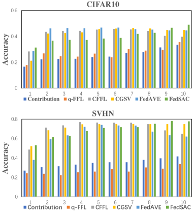
Figure 4.  Comparison results of test accuracy using the data partition of DIR (1.0) with state-of-the-art methods in CIFAR10 (up) and SVHN (down). Results of other scenes are in Appendix D.

Predictive performance (RQ2). To effectively assess the predictive performance of algorithms, we present our highest test accuracies in comparison with all baseline methods in Table 2. These results demonstrate the ability of the algorithms to reward high-contributing clients with high-performance. First, comparing the accuracy of FedSAC with Standalone (i.e., contribution) reveals that FedSAC significantly outperforms Standalone. Second, among the POW scene, FedSAC achieves the highest performance in CIFAR10, SVHN and Fashion MNIST with accuracies of 48.61%, 74.84%, and 87.88%, respectively. Third, for the CLA scene on three datasets, the highest accuracy is obtained by FedSAC, surpassing FedAvg by at least 0.19%. In addition, in the extremely non-iid setting (e.g., DIR (1.0) of SVHN), our method outperforms CFFL, CGSV, and FedAVE by 2.17%, 5.06%, and 4.62%, respectively. Finally, for the DIR(2.0), and DIR (3.0) scenes, FedSAC achieves comparable performance to baseline methods in terms of accuracy. Specially, the notably poor accuracy of q-FFL appears attributed to its mechanism that offers the same reward to all clients, without adapting these rewards based on individual client contributions. Figure 4 illustrates the distributions of contributions and allocated rewards under scenes (i.e., DIR (1.0)) in CIFAR10 comparing FedSAC against baseline methods. It demonstrates that FedSAC not only guarantees BCF but also enables clients to receive rewards that exceed their contributions (i.e., Standalone). In short, FedSAC outperforms all baselines in terms of accuracy. More results under different scenarios (i.e., CLA scene) on CIFAR10 and SVHN are presented in Appendix B.

Figure 5 illustrates the changes in clients’ test accuracy as the number of communication rounds increases in the POW, and CLA data partition of CIFAR10 and SVHN. Owing to the varying data sizes and diversity of labels owned by clients in FL, their contributions to the system exhibit significant differences. As shown in Figure 5, our proposed FedSAC, underpinned by a theoretical guarantee, aims to reward high-contributing clients with high-performance submodels by maintaining consistency in local models. As a result, each client will converge to a different model and achieve varying levels of performance.

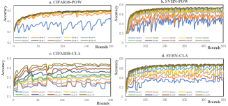
Figure 5. The test accuracy achieved by clients during training for CIFAR10 (left) and SVHN (right) in each round, under the setting of POW and CLA.

Ablation study (RQ3). To evaluate the effectiveness of two proposed modules in FedSAC, a series of ablation experiments are carried out on three public benchmarks with 10 clients, as shown in Table 3 and 4. The operation of eliminating neuron importance, denoted as $w/o$ $allocation$, aims to treat all neurons equally and allocate submodels based on their contributions. $w/o$ $aggregation$ denotes removing the dynamic aggregation module, which uses the traditional FedAvg aggregation method to train. The effectiveness of the submodel allocation module is demonstrated in Table 3, indicating that this module can reward high-contribution clients to obtain high-performance models. In particular, our method has significantly improved the fairness measure by 88.21% on the DIR (1.0) scene of the CIFAR10 dataset. Table 4 shows the results of the proposed dynamic aggregation module, which implies that this module can effectively aggregate submodels with different sizes, thereby further improving the overall performance of the local models. Thus, the ablation study demonstrates that the two designed modules in FedSAC are crucial and significant in enhancing bounded collaborative fairness.

In summary, all experimental results show that both fairness and model accuracy are of significance for bounded collaborative fairness, and our FedSAC outperforms all baseline methods in both fairness and model accuracy.

6. Conclusion

In this work, we introduce a novel FL framework named FedSAC that allocates submodels based on their contributions, thereby ensuring bounded collaborative fairness and attaining superior local accuracy while maintaining the consistency in local models. Our method ensures that high-contributing clients can be rewarded with high-performance submodels, which in turn enhances the overall model accuracy. The experiments on three datasets show that FedSAC exhibits a distinct advantage over baseline methods in terms of fairness and accuracy. In the future, we aim to investigate the implementation of FedSAC on large models.

A. Proof of Theorem 2

Let $I_{E}$ be the set of global synchronization steps, i.e., $I_{E}=\{nE|n=1,2,...\}$. For convenience, We define $v_{i}^{t+1}$ as the immediate result of one step SGD update from $\theta_{i}^{t}$, i.e., $v_{i}^{t+1}=\theta_{i}^{t}-\eta_{t}\nabla F_{i}(\theta_{i}^{t},\xi_{i}^{t})$. $\bar{g}_{t}=\sum_{i=1}^{N}\frac{\nabla F_{i}(\theta_{i}^{t})}{p_{i}}$ and $g_{t}=\sum_{i=1}^{N}\frac{\nabla F_{i}(\theta_{i}^{t},\xi_{i}^{t})}{p_{i}}$. Therefore, $\bar{v}_{t+1}=\bar{\theta}_{t}-\eta_{t}g_{t}$ and $Eg_{t}=\bar{g}_{t}$.

Lemma 1.

(Result of one step SGD). Assume ASSUMPTION 10 and ASSUMPTION 11. If $\eta_{t}\leqslant\frac{1}{4L}$, we have

(20) $$\begin{split}E\|\bar{v}_{t+1}-\theta^{*}\|^{2}&\leqslant(1-\eta_{t}\mu)E\|\bar{\theta}_{t}-\theta^{*}\|^{2}+\eta_{t}^{2}E\|g_{t}-\bar{g}_{t}\|^{2}\\ &\quad+6L\eta_{t}^{2}\Gamma+2E\sum_{i=1}^{N}\frac{\|\bar{\theta}_{t}-\theta_{i}^{t}\|^{2}}{p_{i}},\end{split}$$

where $\Gamma=F^{*}-\sum_{i=1}^{N}\frac{F_{i}^{*}}{p_{i}}$. LAMMA 1 has been made by (Li et al., 2019a).

For Assumption 3, the variance of stochastic gradients within device $i$ is constrained by $\sigma_{i}^{2}$. Consequently,

(21) $$\begin{split}E\|g_{t}-\bar{g}_{t}\|^{2}&=E\|\sum_{i=1}^{N}\frac{1}{p_{i}}(\nabla F_{k}(\theta_{i}^{t},\xi_{i}^{t})-\nabla F_{i}(\theta_{i}^{t}))\|^{2}\\ &=\sum_{i=1}^{N}\frac{1}{p_{i}^{2}}E\|\nabla F_{i}(\theta_{i}^{t},\xi_{i}^{t})-\nabla F_{i}(\theta_{i}^{t})\|^{2}\\ &\leqslant\sum_{i=1}^{N}\frac{1}{p_{i}^{2}}\sigma_{i}^{2}.\end{split}$$

As FedSAC requires communication each $E$ steps. We let $\eta_{t}\leqslant 2\eta_{t+E}$. Therefore, for any $t\geq 0$, there exists a $t_{0}\leqslant t$, such that $t-t_{0}\leqslant E-1$ and $\theta_{i}^{t_{0}}=\bar{\theta}_{t_{0}}$ for all $k=1,2,...,N$. Then

(22) $$\begin{split}E\sum_{i=1}^{N}\frac{1}{p_{i}}\|\bar{\theta}_{t}-\theta_{i}^{t}\|^{2}&=E\sum_{i=1}^{N}\frac{1}{p_{i}}\|(\theta_{i}^{t}-\bar{\theta}_{t_{0}})-(\bar{\theta}_{t}-\bar{\theta}_{t_{0}})\|^{2}\\ &\leqslant E\sum_{i=1}^{N}\frac{1}{p_{i}}\|\theta_{i}^{t}-\bar{\theta}_{t_{0}}\|^{2}\\ &\leqslant E\sum_{t=t_{0}}^{t-1}(E-1)\eta_{t}^{2}\|\nabla F_{k}(\theta_{i}^{t},\xi_{i}^{t})\|^{2}\\ &\leqslant\sum_{t=t_{0}}^{t-1}(E-1)\eta_{t_{0}}^{2}G^{2}\\ &\leqslant\eta_{t_{0}}^{2}(E-1)^{2}G^{2}\\ &\leqslant 4\eta_{t}^{2}(E-1)^{2}G^{2}.\end{split}$$

Here in lines 1252-1256, we use $E\|X-EX\|^{2}\leqslant E\|X\|^{2}$ where $X=\theta_{i}^{t}-\bar{\theta}_{t_{0}}$ with probability $\frac{1}{p_{i}}$. In the lines 1256-1259, we use Jensen inequality:

(23) $$\begin{split}\|\theta_{i}^{t}-\bar{\theta}_{t_{0}}\|&=\|\sum_{t=t_{0}}^{t-1}\eta_{t}\nabla F_{i}(\theta_{i}^{t},\xi_{i}^{t})\|^{2}\\ &\leqslant(t-t_{0})\sum_{t-t_{0}}\sum_{t-t_{0}}^{t-1}\eta_{t}^{2}\|\nabla F_{i}(\theta_{i}^{t},\xi_{i}^{t})\|^{2}.\end{split}$$

In lines 1259-1262, we utilize $\eta_{t}\leqslant\eta_{t_{0}}$ for $t\geq t_{0}$ and $E\|\nabla F_{k}(\theta_{i}^{t},\xi_{i}^{t})\|^{2}\leqslant G^{2}$ for $i=1,2,...,N$. In the lines 1263-1265, we use $\eta_{t_{0}}\leqslant 2\eta_{t_{0}+E}\leqslant 2\eta_{t}$ for $t_{0}\leqslant t\leqslant t_{0}+E$.

Let $\triangle_{t}=E\|\bar{\theta}_{t}-\theta^{*}\|$. Fromr Eq.(20), Eq. (21), and Eq. (22), it follows that

(24) $$\begin{split}\triangle_{t+1}&\leqslant(1-\eta_{t}\mu)\triangle_{t}+\eta_{t}^{2}\sum_{i=1}^{N}\frac{\sigma^{2}}{p_{i}^{2}}+6L\eta_{t}^{2}\Gamma+8\eta_{t}^{2}(E-1)^{2}G^{2}\\ &\leqslant(1-\eta_{t}\mu)\triangle_{t}+\eta_{t}^{2}\underbrace{(\sum_{i=1}^{N}\frac{\sigma^{2}}{p_{i}^{2}}+6L\Gamma+8(E-1)^{2}G^{2})}_{\text{$B$}}\end{split}$$

For a diminishing stepsize, $\eta_{t}=\frac{\kappa}{t+\gamma}$ for some $\kappa>\frac{1}{\mu}$ and $\gamma>0$ such that $\eta_{1}\leqslant min\{\frac{1}{\mu},\frac{1}{4L}\}=\frac{1}{4L}$ and $\eta_{t}\leqslant 2\eta_{t+E}$. We will prove $\triangle\leqslant\frac{v}{\gamma+t}$ by induction, where $v=max\{\frac{\kappa^{2}B}{\kappa\mu-1},(\gamma+1)\triangle_{1}\}$. Firstly, the definition of $v$ guarantees its applicability for $t=1$. Assuming the conclusion holds for some $t$, it follows that

(25) $$\begin{split}\triangle_{t+1}&\leqslant(1-\eta_{t}\mu)\triangle_{t}+\eta_{t}^{2}B\\ &\leqslant(1-\frac{\kappa\mu}{t+\gamma})\frac{v}{t+\gamma}+\frac{\kappa^{2}B}{(t+\gamma)^{2}}\\ &=\frac{t+\gamma-1}{(t+\gamma)^{2}}v+[\frac{\kappa^{2}B}{(t+\gamma)^{2}}-\frac{\kappa\mu-1}{(t+\gamma)^{2}}v]\\ &\leqslant\frac{t+\gamma-1}{(t+\gamma)^{2}}v+\frac{\kappa^{2}B}{(t+\gamma)^{2}}-\frac{\kappa^{2}B}{(t+\gamma)^{2}}\underbrace{-\frac{\kappa\mu-1}{(t+\gamma)^{2}(\gamma+1)\triangle_{1}}}_{\leqslant 0}\\ &\leqslant\frac{v}{t+\gamma-1}\end{split}$$

Then by the $L$-smoothness (ASSUMPTION 10) of $F$,

(26) $$\begin{split}E[F(\bar{\theta}_{T})]-F^{*}&\leqslant(\bar{\theta}_{T}-\theta^{*})^{T}\underbrace{\nabla F_{i}(\theta^{*})}_{=0}+\frac{L}{2}\|\bar{\theta}_{T}-\theta^{*}\|_{2}^{2}\\ &=\frac{L}{2}\triangle_{T}\\ &\leqslant\frac{L}{2}\frac{v}{\gamma+T}\end{split}$$

We let $\kappa=\frac{2}{\mu}$, $\gamma=max\{8\frac{L}{\mu},E\}-1$. In the lines 1293, we have

(27) $$\begin{split}v&=max\{\frac{\kappa^{2}B}{\kappa\mu-1},(\gamma+1)\triangle_{1}\}\\ &\leqslant\frac{\kappa^{2}B}{\kappa\mu-1}+(\gamma+1)\triangle_{1}\\ &\leqslant\frac{4B}{\mu^{2}}+(\gamma+1)\triangle_{1}\end{split}$$

Substituting Eq. 27 into Eq. 26, we obtain

(28) $$\begin{split}0\leqslant\lim_{T\to\infty}E[F(\bar{\theta}_{T})]-F^{*}\leqslant\lim_{T\to\infty}[\frac{L}{\gamma+T}(\frac{2B}{\mu^{2}}+\frac{\gamma+1}{2}\triangle_{1})]=0\end{split}$$

Therefore, $\lim\limits_{T\to\infty}E[F(\bar{\theta}_{T})]-F^{*}=0$.

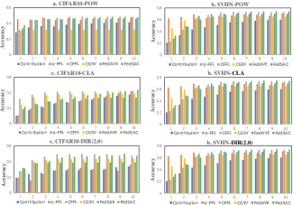
Figure 6.  Comparison results of test accuracy using the scene of POW, CLA, and DIR(2.0) with state-of-the-art methods in CIFAR10 (left) and SVHN (right). In terms of accuracy across clients, FedSAC exhibits the highest level of consistency with the contribution.

Dataset	CIFAR10									Fashion MNIST
No. Clients	20					40		60		20
Scene	POW	CLA	DIR(1.0)	DIR(2.0)	DIR(3.0)	DIR(1.0)	DIR(2.0)	DIR(1.0)	DIR(2.0)	POW	CLA	DIR(1.0)	DIR(2.0)	DIR(3.0)
FedAvg(McMahan et al., 2017)	-40.52$\pm$3.3	83.57$\pm$1.4	18.41$\pm$16.3	77.52$\pm$1.5	44.13$\pm$16.0	79.53$\pm$13.9	54.37$\pm$11.1	51.64$\pm$17.8	55.22$\pm$6.8	-34.64$\pm$5.6	84.37$\pm$3.3	22.95$\pm$2.6	30.39$\pm$6.7	56.37$\pm$3.5
q-FFL(Li et al., 2019b)	14.10$\pm$2.8	98.09$\pm$0.2	83.98$\pm$2.0	86.14$\pm$2.9	90.00$\pm$0.5	87.81$\pm$1.6	80.46$\pm$1.1	80.65$\pm$2.9	85.76$\pm$1.2	29.24$\pm$5.3	98.44$\pm$2.6	81.75$\pm$4.8	77.45$\pm$5.6	72.89$\pm$3.9
CFFL(Lyu et al., 2020b)	81.45$\pm$1.0	95.93$\pm$0.8	76.72$\pm$2.1	76.09$\pm$1.3	63.79$\pm$0.5	50.33$\pm$1.2	49.61$\pm$0.6	86.59$\pm$1.3	87.52$\pm$0.5	88.02$\pm$0.4	92.29$\pm$2.5	72.74$\pm$2.4	78.40$\pm$1.2	75.36$\pm$1.6
CGSV(Xu et al., 2021)	83.30$\pm$1.8	96.80$\pm$0.1	79.85$\pm$0.9	79.73$\pm$1.3	85.72$\pm$0.4	82.90$\pm$0.4	80.47$\pm$0.7	85.91$\pm$1.2	77.91$\pm$0.8	83.85$\pm$0.4	94.04$\pm$0.8	88.32$\pm$2.5	83.68$\pm$1.1	74.15$\pm$1.7
FedAVE(Wang et al., 2024)	88.46$\pm$1.5	97.18$\pm$0.6	87.59$\pm$1.1	78.43$\pm$0.4	68.70$\pm$1.3	45.69$\pm$2.6	65.60$\pm$1.2	38.92$\pm$1.1	60.61$\pm$1.3	87.14$\pm$0.6	93.97$\pm$1.2	78.87$\pm$2.1	81.20$\pm$1.5	72.73$\pm$0.7
Ours	99.62$\pm$0.2	98.52$\pm$0.1	96.29$\pm$0.4	98.06$\pm$0.5	95.99$\pm$0.4	99.37$\pm$0.5	96.57$\pm$0.2	97.69$\pm$0.6	95.12$\pm$0.3	97.40$\pm$0.4	98.49$\pm$0.3	96.52$\pm$0.8	97.65$\pm$0.6	96.47$\pm$0.7

Table 5.  Comparison results of fairness $\rho\in[-100,100]$ with state-of-the-art methods on CIFAR10 and Fashion MNIST. The reported results are averaged over 5 runs with different random seeds. (A higher value indicates better fairness. The best average result is marked in bold. The second-best result is underlined. These notes are the same to others.)

Dataset	CIFAR10									Fashion MNIST
No. Clients	20					40		60		20
Scene	POW	CLA	DIR(1.0)	DIR(2.0)	DIR(3.0)	DIR(1.0)	DIR(2.0)	DIR(1.0)	DIR(2.0)	POW	CLA	DIR(1.0)	DIR(2.0)	DIR(3.0)
Standalone	37.15$\pm$0.0	35.25$\pm$0.3	27.82$\pm$0.0	31.83$\pm$0.1	33.56$\pm$0.1	32.13$\pm$0.1	28.86$\pm$0.2	28.58$\pm$0.2	27.84$\pm$0.1	82.36$\pm$0.1	81.17$\pm$0.2	66.71$\pm$0.2	68.00$\pm$0.2	73.63$\pm$0.3
FedAvg(McMahan et al., 2017)	46.94$\pm$0.2	41.14$\pm$0.6	48.31$\pm$0.5	49.00$\pm$0.5	50.13$\pm$0.3	48.19$\pm$0.3	49.57$\pm$0.3	49.06$\pm$0.1	49.30$\pm$0.3	87.29$\pm$0.3	84.67$\pm$0.2	87.46$\pm$0.0	88.06$\pm$0.1	88.04$\pm$0.1
q-FFL(Li et al., 2019b)	46.87$\pm$0.2	41.56$\pm$0.3	33.77$\pm$0.1	38.17$\pm$0.9	43.91$\pm$0.6	38.64$\pm$1.5	39.37$\pm$0.4	34.01$\pm$0.1	36.77$\pm$0.5	85.79$\pm$0.2	81.10$\pm$0.1	68.30$\pm$1.7	78.59$\pm$1.8	77.69$\pm$1.1
CFFL(Lyu et al., 2020b)	46.06$\pm$0.0	39.43$\pm$0.3	45.76$\pm$0.3	48.57$\pm$0.2	48.42$\pm$0.3	39.54$\pm$0.3	39.16$\pm$0.6	42.33$\pm$0.4	41.06$\pm$0.6	85.88$\pm$1.8	81.75$\pm$2.1	81.69$\pm$0.6	84.16$\pm$0.4	87.34$\pm$0.4
CGSV(Xu et al., 2021)	46.29$\pm$0.2	37.75$\pm$1.4	46.72$\pm$1.0	48.45$\pm$0.3	49.24$\pm$0.2	46.75$\pm$0.2	48.32$\pm$0.1	49.11$\pm$0.7	48.58$\pm$0.3	87.21$\pm$0.2	84.25$\pm$0.2	85.17$\pm$0.7	86.85$\pm$0.3	88.07$\pm$0.2
FedAVE(Wang et al., 2024)	46.43$\pm$0.6	40.99$\pm$0.2	46.64$\pm$0.6	48.34$\pm$0.5	48.13$\pm$0.6	46.58$\pm$0.4	46.73$\pm$0.3	47.29$\pm$0.8	49.21$\pm$0.6	87.44$\pm$0.1	84.79$\pm$0.5	79.53$\pm$0.9	84.47$\pm$0.4	86.83$\pm$0.1
Ours	48.60$\pm$0.7	43.39$\pm$0.2	49.41$\pm$0.1	49.09$\pm$0.1	50.48$\pm$0.1	48.64$\pm$0.3	49.68$\pm$0.4	49.23$\pm$0.1	49.34$\pm$0.2	87.60$\pm$0.1	84.99$\pm$0.3	87.57$\pm$0.6	88.08$\pm$0.3	88.17$\pm$0.3

Table 6.  Comparison results of the maximum test accuracy ($\%$) with state-of-the-art methods on CIFAR10 and Fashion MNIST. The reported results are averaged over 5 runs with different random seeds. (A higher value indicates better accuracy.)

B. Final Rewards of Clients

Figure 6 shows the distributions of contributions and the final rewards of clients under different scenes (i.e., POW, CLA, DIR (2.0) in CIFAR10 and SVHN) by FedSAC and the compared methods. Existing methods allocate rewards to clients lack sufficient differentiation, resulting in an ongoing unfairness for high-contributing clients. For example in SVHN-CLA (Figure 6 (d)), the contributions (i.e., Standalone) of $Client_{3}$ and $Client_{10}$ differ significantly. However, CFFL and CGSV do not exhibit a substantial difference in the rewards assigned to them. In addition, FedSAC effectively differentiates the rewards it received, thereby ensuring the collaborative fairness in FL.

Scene	POW	DIR(1.0)	DIR(2.0)	DIR(3.0)
$FedSAC(\beta=2)$	49.23(44.77)	49.66(39.53)	50.60(37.87)	51.37(43.19)
$FedSAC(\beta=5)$	48.43(37.73)	49.10(35.76)	50.01(30.91)	49.85(38.46)
$FedSAC(\beta=10)$	48.61(30.91)	49.06(31.36)	47.08(23.72)	49.04(28.54)
$FedSAC(\beta=20)$	46.53(24.10)	46.98(28.41)	43.50(20.17)	46.03(25.70)

Table 7. The maximum test accuracy (%) achieved by FedSAC across different $\beta$, given a fairness threshold of $\rho>95\%$, on CIFAR10. Values in the middle brackets represent the minimum test accuracy (%) among 10 clients.

Dataset	CIFAR10					SVHN					Fashion MNIST
No. Clients	10					10					10
Scene	POW	CLA	DIR(1.0)	DIR(2.0)	DIR(3.0)	POW	CLA	DIR(1.0)	DIR(2.0)	DIR(3.0)	POW	CLA	DIR(1.0)	DIR(2.0)	DIR(3.0)
FedAvg(McMahan et al., 2017)	26.27	26.27	26.27	26.27	26.27	26.27	26.27	26.27	26.27	26.27	7.97	7.97	7.97	7.97	7.97
q-FFL(Li et al., 2019b)	26.27	26.27	26.27	26.27	26.27	26.27	26.27	26.27	26.27	26.27	7.97	7.97	7.97	7.97	7.97
CFFL(Lyu et al., 2020b)	26.27	26.27	26.27	26.27	26.27	26.27	26.27	26.27	26.27	26.27	7.97	7.97	7.97	7.97	7.97
CGSV(Xu et al., 2021)	26.27	26.27	26.27	26.27	26.27	26.27	26.27	26.27	26.27	26.27	7.97	7.97	7.97	7.97	7.97
FedAVE(Wang et al., 2024)	26.27	26.27	26.27	26.27	26.27	26.27	26.27	26.27	26.27	26.27	7.97	7.97	7.97	7.97	7.97
Ours	23.57	23.58	23.39	24.02	23.63	20.86	22.31	23.85	15.51	21.75	6.89	7.28	5.30	4.77	5.23

Table 8. Comparison on communication costs (MB per round) of FedSAC and the baselines framework.

Dataset	CIFAR10					SVHN					Fashion MNIST
No. Clients	10					10					10
Scene	POW	CLA	DIR(1.0)	DIR(2.0)	DIR(3.0)	POW	CLA	DIR(1.0)	DIR(2.0)	DIR(3.0)	POW	CLA	DIR(1.0)	DIR(2.0)	DIR(3.0)
$\eta$	0.05	0.05	0.05	0.03	0.03	0.03	0.05	0.05	0.05	0.05	0.1	0.05	0.05	0.05	0.05
$E$	15	20	20	20	20	20	20	20	20	20	20	20	20	20	15
$\beta$	5	3	10	2	10	5	3	5	10	5	10	1	10	20	25

Table 9. The optimal hyperparameters in given scenarios. Learning rate $\eta$, the number of local update steps $E$, hyper-parameter $\beta$. Batch sizes $B$ are set as 32, 64, and 32 for CIFAR10, SVHN, and FashionMNIST, respectively.

C. Varying Numbers of Clients

To verify the effectiveness of FedSAC in scenarios with varying numbers of clients, we conduct experiments by increasing the number of local clients to 20, 40, and 60, respectively. Table 5 presents the fairness results achieved by FedSAC and the compared methods, while Table 6 shows the maximum local model performance achieved by these methods. In the large client number settings (No. Clients = 20, 40, and 60), FedSAC outperforms all baseline methods in terms of fairness (refer to Table 5) and accuracy (refer to Table 6). The results demonstrate that FedSAC can effectively implement bounded collaborative fairness in scenarios with varying numbers of clients.

D. The Impact of $\beta$ on The Experiment

In Table 7, we present the performance of FedSAC with different values of $\beta$ on each scene of CIFAR10. The experiments demonstrate that as $\beta$ increases, the maximum test accuracy will gradually decrease. This is because the size of the submodels downloaded by clients increases as $\beta$ decreases. When $\beta$ is small, the submodels of low-contribution clients contain more neurons, enabling effective training to enhance all local model performance.

E. The Communication Cost Experiments

The most works on collaborative fairness require full clients’ information (Lyu et al., 2020b; Xu and Lyu, 2020; Xu et al., 2021), which will inevitably introduce large communication overhead and computation cost. In addition, this communication and computation overhead of full sampling problem is tolerable for most cases in cross-silo FL scenarios  (Du Terrail et al., 2022), such as healthcare and finance, because there are only dozens of clients in cross-silo FL scenarios. In the Table 8, the results show that our FedSAC demonstrates less communication costs than all the baseline methods in three datasets across all settings. In addition, our FedSAC does not introduce additional communication, because the evaluation of neuron importance is conducted on the server without communicating with clients, effectively preventing any communication overhead. In the Table 8, FedSAC exhibits a communication complexity of O(d*m) per round (Horvath et al., 2021), where m$<$=1 represents the average ratio of the parameters of the submodel compared to the global model. In conclusion, all baseline methods show a higher communication complexity of O(d) than FedSAC.

F. Details on Hyper-parameters

For each dataset, the local data of each client was partitioned into training and validation sets. Then, we tuned each dataset hyper-parameters by using grid search with FedAvg. Subsequently, we applied the optimal parameters obtained from the validation dataset. The optimized hyper-parameters for scenarios (i.e., POW, CLA, DIR(1.0), DIR(2.0), and DIR(3.0)) are shown in Table 9.

References

- (1)
- Agarwal et al. (2019) Anish Agarwal et al. 2019. A marketplace for data: An algorithmic solution. In Proceedings of the 2019 ACM Conference on Economics and Computation. 701–726.
- Chen et al. (2022) Chen Chen et al. 2022. Gear: a margin-based federated adversarial training approach. In International Workshop on Trustable, Verifiable, and Auditable Federated Learning in Conjunction with AAAI, Vol. 2022.
- Chen et al. (2023) Dengsheng Chen, Jie Hu, Vince Junkai Tan, Xiaoming Wei, and Enhua Wu. 2023. Elastic Aggregation for Federated Optimization. In Proceedings of the IEEE/CVF Conference on Computer Vision and Pattern Recognition (CVPR). 12187–12197.
- Du Terrail et al. (2022) Jean Ogier Du Terrail, Samy-Safwan Ayed, Edwige Cyffers, Felix Grimberg, Chaoyang He, Regis Loeb, Paul Mangold, Tanguy Marchand, Othmane Marfoq, Erum Mushtaq, et al. 2022. FLamby: Datasets and Benchmarks for Cross-Silo Federated Learning in Realistic Healthcare Settings. In NeurIPS 2022-Thirty-sixth Conference on Neural Information Processing Systems.
- Gao et al. (2022a) Liang Gao, Huazhu Fu, Li Li, Yingwen Chen, Ming Xu, and Cheng-Zhong Xu. 2022a. FedDC: Federated Learning With Non-IID Data via Local Drift Decoupling and Correction. In Proceedings of the IEEE/CVF Conference on Computer Vision and Pattern Recognition (CVPR). 10112–10121.
- Gao et al. (2022b) Liang Gao, Huazhu Fu, Li Li, Yingwen Chen, Ming Xu, and Cheng-Zhong Xu. 2022b. Feddc: Federated learning with non-iid data via local drift decoupling and correction. In Proceedings of the IEEE/CVF Conference on Computer Vision and Pattern Recognition. 10112–10121.
- Hong et al. (2022) Junyuan Hong, Haotao Wang, Zhangyang Wang, and Jiayu Zhou. 2022. Efficient Split-Mix Federated Learning for On-Demand and In-Situ Customization. In In Proceedings of the International Conference on Learning Representations.
- Horvath et al. (2021) Samuel Horvath, Stefanos Laskaridis, Mario Almeida, Ilias Leontiadis, Stylianos Venieris, and Nicholas Lane. 2021. Fjord: Fair and accurate federated learning under heterogeneous targets with ordered dropout. Advances in Neural Information Processing Systems 34 (2021), 12876–12889.
- Huang et al. (2022) Wenke Huang, Mang Ye, and Bo Du. 2022. Learn From Others and Be Yourself in Heterogeneous Federated Learning. In Proceedings of the IEEE/CVF Conference on Computer Vision and Pattern Recognition (CVPR). 10143–10153.
- Huang et al. (2021) Yutao Huang, Lingyang Chu, Zirui Zhou, Lanjun Wang, Jiangchuan Liu, Jian Pei, and Yong Zhang. 2021. Personalized cross-silo federated learning on non-iid data. In Proceedings of the AAAI conference on artificial intelligence, Vol. 35. 7865–7873.
- Khramtsova et al. (2020) Ekaterina Khramtsova, Christian Hammerschmidt, Sofian Lagraa, and Radu State. 2020. Federated learning for cyber security: SOC collaboration for malicious URL detection. In 2020 IEEE 40th International Conference on Distributed Computing Systems (ICDCS). IEEE, 1316–1321.
- Krizhevsky et al. (2009) Alex Krizhevsky, Geoffrey Hinton, et al. 2009. Learning multiple layers of features from tiny images. Master’s thesis, Department of Computer Science, University of Toronto, 2009. (2009).
- LeCun et al. (1998) Yann LeCun, Léon Bottou, Yoshua Bengio, and Patrick Haffner. 1998. Gradient-based learning applied to document recognition. Proc. IEEE 86, 11 (1998), 2278–2324.
- Li et al. (2021) Ang Li, Jingwei Sun, Xiao Zeng, Mi Zhang, Hai Li, and Yiran Chen. 2021. Fedmask: Joint computation and communication-efficient personalized federated learning via heterogeneous masking. In Proceedings of the 19th ACM Conference on Embedded Networked Sensor Systems. 42–55.
- Li et al. (2023) Bo Li, Mikkel N. Schmidt, Tommy S. Alstrøm, and Sebastian U. Stich. 2023. On the Effectiveness of Partial Variance Reduction in Federated Learning With Heterogeneous Data. In Proceedings of the IEEE/CVF Conference on Computer Vision and Pattern Recognition (CVPR). 3964–3973.
- Li et al. (2020) Tian Li, Anit Kumar Sahu, Manzil Zaheer, Maziar Sanjabi, Ameet Talwalkar, and Virginia Smith. 2020. Federated optimization in heterogeneous networks. Proceedings of Machine learning and systems 2 (2020), 429–450.
- Li et al. (2019b) Tian Li, Maziar Sanjabi, Ahmad Beirami, and Virginia Smith. 2019b. Fair Resource Allocation in Federated Learning. In International Conference on Learning Representations.
- Li et al. (2019a) Xiang Li, Kaixuan Huang, Wenhao Yang, Shusen Wang, and Zhihua Zhang. 2019a. On the Convergence of FedAvg on Non-IID Data. In International Conference on Learning Representations.
- Lin et al. (2020) Tao Lin, Lingjing Kong, Sebastian U Stich, and Martin Jaggi. 2020. Ensemble distillation for robust model fusion in federated learning. Advances in Neural Information Processing Systems 33 (2020), 2351–2363.
- Luo et al. (2017) Jian-Hao Luo et al. 2017. Thinet: A filter level pruning method for deep neural network compression. In Proceedings of the IEEE international conference on computer vision. 5058–5066.
- Lyu et al. (2020a) Lingjuan Lyu, Yitong Li, Karthik Nandakumar, Jiangshan Yu, and Xingjun Ma. 2020a. How to democratise and protect AI: Fair and differentially private decentralised deep learning. IEEE Transactions on Dependable and Secure Computing (2020).
- Lyu et al. (2020b) Lingjuan Lyu, Xinyi Xu, Qian Wang, and Han Yu. 2020b. Collaborative fairness in federated learning. In Federated Learning. Springer, 189–204.
- McMahan et al. (2017) Brendan McMahan, Eider Moore, Daniel Ramage, Seth Hampson, and Blaise Aguera y Arcas. 2017. Communication-efficient learning of deep networks from decentralized data. In Artificial Intelligence and Statistics. PMLR, 1273–1282.
- Mendieta et al. (2022) Matias Mendieta, Taojiannan Yang, Pu Wang, Minwoo Lee, Zhengming Ding, and Chen Chen. 2022. Local Learning Matters: Rethinking Data Heterogeneity in Federated Learning. In Proceedings of the IEEE/CVF Conference on Computer Vision and Pattern Recognition (CVPR). 8397–8406.
- Molchanov et al. (2019) Pavlo Molchanov, Arun Mallya, Stephen Tyree, Iuri Frosio, and Jan Kautz. 2019. Importance estimation for neural network pruning. In Proceedings of the IEEE/CVF Conference on Computer Vision and Pattern Recognition. 11264–11272.
- Molchanov et al. (2017) Pavlo Molchanov, Stephen Tyree, Tero Karras, Timo Aila, and Jan Kautz. 2017. Pruning Convolutional Neural Networks for Resource Efficient Inference. In In Proceedings of the International Conference on Learning Representations.
- Netzer et al. (2011) Yuval Netzer, Tao Wang, Adam Coates, Alessandro Bissacco, Bo Wu, and Andrew Y Ng. 2011. Reading digits in natural images with unsupervised feature learning. In NIPS Workshop on Deep Learning and Unsupervised Feature Learning 2011 (2011).
- Ogier du Terrail et al. (2022) Jean Ogier du Terrail, Samy-Safwan Ayed, Edwige Cyffers, Felix Grimberg, Chaoyang He, Regis Loeb, Paul Mangold, Tanguy Marchand, Othmane Marfoq, Erum Mushtaq, et al. 2022. FLamby: Datasets and Benchmarks for Cross-Silo Federated Learning in Realistic Healthcare Settings. Advances in Neural Information Processing Systems 35 (2022), 5315–5334.
- Qin et al. (2023) Zhen Qin, Shuiguang Deng, Mingyu Zhao, and Xueqiang Yan. 2023. FedAPEN: Personalized Cross-silo Federated Learning with Adaptability to Statistical Heterogeneity. In Proceedings of the 29th ACM SIGKDD Conference on Knowledge Discovery and Data Mining. 1954–1964.
- Richardson et al. (2020) Adam Richardson et al. 2020. Budget-bounded incentives for federated learning. In Federated Learning. Springer, 176–188.
- Shi et al. (2021) Yuxin Shi et al. 2021. A survey of fairness-aware federated learning. arXiv preprint arXiv:2111.01872 (2021).
- Shi et al. (2023) Yuxin Shi, Han Yu, and Cyril Leung. 2023. Towards fairness-aware federated learning. IEEE Transactions on Neural Networks and Learning Systems (2023).
- Sim et al. (2020) Rachael Hwee Ling Sim, Yehong Zhang, Mun Choon Chan, and Bryan Kian Hsiang Low. 2020. Collaborative machine learning with incentive-aware model rewards. In International Conference on Machine Learning. PMLR, 8927–8936.
- Stich (2018) Sebastian U Stich. 2018. Local SGD converges fast and communicates little. arXiv preprint arXiv:1805.09767 (2018).
- Stich et al. (2018) Sebastian U Stich, Jean-Baptiste Cordonnier, and Martin Jaggi. 2018. Sparsified SGD with memory. Advances in Neural Information Processing Systems 31 (2018).
- Sun et al. (2021) Benyuan Sun, Hongxing Huo, Yi Yang, and Bo Bai. 2021. Partialfed: Cross-domain personalized federated learning via partial initialization. Advances in Neural Information Processing Systems 34 (2021), 23309–23320.
- Tan et al. (2023) Yue Tan, Yixin Liu, Guodong Long, Jing Jiang, Qinghua Lu, and Chengqi Zhang. 2023. Federated learning on non-iid graphs via structural knowledge sharing. In Proceedings of the AAAI conference on artificial intelligence, Vol. 37. 9953–9961.
- Tay et al. (2022) Sebastian Shenghong Tay, Xinyi Xu, Chuan Sheng Foo, and Bryan Kian Hsiang Low. 2022. Incentivizing collaboration in machine learning via synthetic data rewards. In Proceedings of the AAAI Conference on Artificial Intelligence, Vol. 36. 9448–9456.
- Uddin et al. (2020) Md Palash Uddin, Yong Xiang, Xuequan Lu, John Yearwood, and Longxiang Gao. 2020. Mutual information driven federated learning. IEEE Transactions on Parallel and Distributed Systems 32, 7 (2020), 1526–1538.
- Wang et al. (2020) Tianhao Wang, Johannes Rausch, Ce Zhang, Ruoxi Jia, and Dawn Song. 2020. A principled approach to data valuation for federated learning. Federated Learning: Privacy and Incentive (2020), 153–167.
- Wang et al. (2023) Yangyang Wang, Xiao Zhang, Mingyi Li, Tian Lan, Huashan Chen, Hui Xiong, Xiuzhen Cheng, and Dongxiao Yu. 2023. Theoretical Convergence Guaranteed Resource-Adaptive Federated Learning with Mixed Heterogeneity. In Proceedings of the 29th ACM SIGKDD Conference on Knowledge Discovery and Data Mining. 2444–2455.
- Wang et al. (2024) Zihui Wang, Zhaopeng Peng, Xiaoliang Fan, Zheng Wang, Shangbin Wu, Rongshan Yu, Peizhen Yang, Chuanpan Zheng, and Cheng Wang. 2024. FedAVE: Adaptive data value evaluation framework for collaborative fairness in federated learning. Neurocomputing (2024), 127227.
- Xu and Lyu (2020) Xinyi Xu and Lingjuan Lyu. 2020. A reputation mechanism is all you need: Collaborative fairness and adversarial robustness in federated learning. arXiv preprint arXiv:2011.10464 (2020).
- Xu et al. (2021) Xinyi Xu, Lingjuan Lyu, Xingjun Ma, Chenglin Miao, Chuan Sheng Foo, and Bryan Kian Hsiang Low. 2021. Gradient driven rewards to guarantee fairness in collaborative machine learning. Advances in Neural Information Processing Systems 34 (2021), 16104–16117.
- Xu et al. (2023) Yuan-Yi Xu, Ci-Siang Lin, and Yu-Chiang Frank Wang. 2023. Bias-Eliminating Augmentation Learning for Debiased Federated Learning. In Proceedings of the IEEE/CVF Conference on Computer Vision and Pattern Recognition (CVPR). 20442–20452.
- Yan et al. (2023) Gang Yan, Hao Wang, Xu Yuan, and Jian Li. 2023. Criticalfl: A critical learning periods augmented client selection framework for efficient federated learning. In Proceedings of the 29th ACM SIGKDD Conference on Knowledge Discovery and Data Mining. 2898–2907.
- Yang et al. (2019) Qiang Yang, Yang Liu, Tianjian Chen, and Yongxin Tong. 2019. Federated machine learning: Concept and applications. ACM Transactions on Intelligent Systems and Technology (TIST) 10, 2 (2019), 1–19.
- Yu et al. (2020) Han Yu, Zelei Liu, Yang Liu, Tianjian Chen, Mingshu Cong, Xi Weng, Dusit Niyato, and Qiang Yang. 2020. A fairness-aware incentive scheme for federated learning. In Proceedings of the AAAI/ACM Conference on AI, Ethics, and Society. 393–399.
- Yu et al. (2019) Hao Yu, Sen Yang, and Shenghuo Zhu. 2019. Parallel restarted SGD with faster convergence and less communication: Demystifying why model averaging works for deep learning. In Proceedings of the AAAI Conference on Artificial Intelligence, Vol. 33. 5693–5700.
- Yu et al. (2018) Ruichi Yu, Ang Li, Chun-Fu Chen, Jui-Hsin Lai, Vlad I Morariu, Xintong Han, Mingfei Gao, Ching-Yung Lin, and Larry S Davis. 2018. Nisp: Pruning networks using neuron importance score propagation. In Proceedings of the IEEE conference on computer vision and pattern recognition. 9194–9203.
- Yu et al. (2022) Yaodong Yu, Alexander Wei, Sai Praneeth Karimireddy, Yi Ma, and Michael Jordan. 2022. TCT: Convexifying federated learning using bootstrapped neural tangent kernels. Advances in Neural Information Processing Systems 35 (2022), 30882–30897.
- Yurochkin et al. (2019) Mikhail Yurochkin, Mayank Agarwal, Soumya Ghosh, Kristjan Greenewald, Nghia Hoang, and Yasaman Khazaeni. 2019. Bayesian nonparametric federated learning of neural networks. In International Conference on Machine Learning. PMLR, 7252–7261.
- Zhan et al. (2021) Yufeng Zhan, Jie Zhang, Zicong Hong, Leijie Wu, Peng Li, and Song Guo. 2021. A survey of incentive mechanism design for federated learning. IEEE Transactions on Emerging Topics in Computing (2021).
- Zhang et al. (2023) Jianqing Zhang, Yang Hua, Hao Wang, Tao Song, Zhengui Xue, Ruhui Ma, and Haibing Guan. 2023. Fedala: Adaptive local aggregation for personalized federated learning. In Proceedings of the AAAI Conference on Artificial Intelligence, Vol. 37. 11237–11244.
- Zhang et al. (2021) Jingwen Zhang, Yuezhou Wu, and Rong Pan. 2021. Incentive mechanism for horizontal federated learning based on reputation and reverse auction. In Proceedings of the Web Conference 2021. 947–956.
- Zhang et al. (2012) Yuchen Zhang, Martin J Wainwright, and John C Duchi. 2012. Communication-efficient algorithms for statistical optimization. Advances in neural information processing systems 25 (2012).