MODL: Multilearner Online Deep Learning

Abstract

Online deep learning solves the problem of learning from streams of data, reconciling two opposing objectives: learn fast and learn deep. Existing work focuses almost exclusively on exploring pure deep learning solutions, which are much better suited to handle the “deep” than the “fast” part of the online learning equation. In our work, we propose a different paradigm, based on a hybrid multilearner approach. First, we develop a fast online logistic regression learner. This learner does not rely on backpropagation. Instead, it uses closed form recursive updates of model parameters, handling the fast learning part of the online learning problem. We then analyze the existing online deep learning theory and show that the widespread ODL approach, currently operating at complexity $O(L^{2})$ in terms of the number of layers $L$, can be equivalently implemented in $O(L)$ complexity. This further leads us to the cascaded multilearner design, in which multiple shallow and deep learners are co-trained to solve the online learning problem in a cooperative, synergistic fashion. We show that this approach achieves state-of-the-art results on common online learning datasets, while also being able to handle missing features gracefully. Our code is publicly available at https://github.com/AntonValk/MODL.

1 Introduction

Off-line machine learning algorithms are trained on bulk datasets, making multiple passes over them to gradually tune model parameters. In many cases it is desirable to be able to learn from data streams, processing each instance sequentially, in a process known as Online Learning (Bottou, 1998). Compared to batch training, online learning allows scalable and memory efficient training regimes, with potentially unbounded dataset sizes. Online learning techniques have been a research area for decades, spanning both supervised (Zinkevich, 2003), semi-supervised (Belkin et al., 2006) and unsupervised learning (Guha et al., 2000) archetypes. Early techniques focused on shallow learners that learn fast, but have limited expressive ability (Hoi et al., 2013). In contrast, deep neural networks provide unlimited expressive power, but their learning tends to be very slow. Sahoo et al. (2018) address this by introducing the ODL (online deep learning) paradigm that jointly learns neural network parameters and the architecture “hedge” weights. ODL is rooted in Hedge backpropagation (Freund and Schapire, 1997) that oscillates between standard backpropagation and the hedge optimization step that updates the scalar weights that link deep neural network early exit points with the final layer. More recently, Agarwal et al. (2023) relied on ODL to address the issue of unreliable features in the data stream. Though these two approaches partially alleviate the issues with training neural networks online, they still suffer from computational complexity and stability issues due to reliance on hedge backpropagation. Indeed, at a certain abstraction level, hedge backpropagation has a tint of a joint architecture learning task, consisting of two optimization objectives (hedge weights and neural network weights) that interfere with each other, making learning slower.

Contributions. In our current work we address these inefficiencies by introducing MODL, a multilearner online deep learning paradigm. This paradigm is based on the following key inductive biases: (i) learners must learn in parallel, removing cross-learner dependencies as much as possible; (ii) backpropagation is slow, therefore some learners can benefit from efficient statistical approximations, making them learn extremely fast, in a closed form recursive style; (iii) combining learner outputs using a delta-regime makes their learning cooperative and synergistic. In the nutshell, our contributions are threefold: (i) MODL achieves state-of-the-art convergence speed and accuracy on standard benchmarks; (ii) we derive a fast recursive logistic regression algorithm that continuously learns on a stream of data; and (iii) we reduce training complexity of the existing ODL method from $O(L^{2})$ to $O(L)$ by analyzing its backpropagation and removing unnecessary complexities.

2 Related Work

Online learning. Early online learning work with statistical methods dates back at least to Bottou (1998). A notable result from Bottou and LeCun (2003) shows that online learning algorithms can be at least as efficient learners as standard full batch methods. First-order gradient based algorithms have long been used in online learning due to their simplicity (Zinkevich, 2003; Bartlett et al., 2007). Second-order methods strive to increase convergence speed, but suffer from high computational cost (Hazan et al., 2007; Dredze et al., 2008). Sahoo et al. (2018) propose a hedge-backpropagation style update to jointly learn the optimal neural network architecture and parameters to dynamically change the model depth as more data become available. Learning from a stream can mean that feature reliability is questionable. Initial approaches that address online learning with haphazard features focused on non-deep learning techniques (Beyazit et al., 2019; He et al., 2019). More recently, a scalable approach for online deep learning with unreliable features was proposed by Agarwal et al. (2023). Online logistic regression was studied by Agarwal et al. (2021), who proposed FOLKLORE, an iterative optimization scheme that still lacks the closed form updates that are needed to improve efficiency. de Vilmarest and Wintenberger (2021) studied online optimization using extended Kalman filter framework with applications to online GLM models. In this work we derive the online logistic regression directly from the Bayesian approximation of posterior.

Applications. There are three primary application areas of Online Learning. First, there are settings where storing training data can be undesirable. Privacy is a well established human right that is all too often violated due to data breaches. A good way to alleviate the danger of exposing sensitive data is to use them for training but never store them at all (Yang et al., 2022). This necessitates the ability to train models from scratch in a single pass over the data (Min et al., 2022). Second, in massive data generating processes, it is physically impossible to store all the generated data, and thus learning has to be performed online as old data are deleted. One such example is the enormous amount of data generated during physics experiments at CERN (Basaglia et al., 2023). CERN only retains a small fraction of data in permanent tapes, while discarding TeraBytes of data after temporary storage. Models can train from these massive data streams online as new data arrive and old data are deleted. Third, Online Learning is particularly useful for model adaptation when there is a mismatch between training datasets and deployment settings. Due to the difficulty in obtaining data in medical settings, it is often necessary to train on a small initial dataset and continue training online as new data arrive (Graas et al., 2023). Even when large amounts of data are available in computer vision settings (Li et al., 2020), online learning techniques are necessary to adjust the model in the presence of distribution shift. Online learning to address distribution shifts is also useful in analyzing power systems (Hu et al., 2021) and addressing non-stationary noise (Liu et al., 2022). Distribution drift can also necessitate online learning to adapt to dynamic settings for tasks like the detection of bad actors in Internet-of-Things networks (Zhang et al., 2020; Shao et al., 2021; Abdel Wahab, 2022).

3 Online Learning with Missing Features

3.1 Problem Satement

We address the Online Learning task with data streams that contain potentially missing features. In this problem setting the data generating process produces a sequence of triplets $\mathcal{P}=\{(\mathbf{z}_{1},\mathbf{y}_{1},\bm{\Omega}_{1}),\dots,(\mathbf{z}_{T},\mathbf{y}_{T},\bm{\Omega}_{T})\}$ sampled sequentially in $T$ time steps. $\mathcal{P}$ consists of input features $\mathbf{z}_{t}\in\mathbb{R}^{d}$, ground truth $\mathbf{y}_{t}\in\mathcal{Y}$ (where $\mathcal{Y}$ has a fixed dimension and may be discrete or continuous depending on the task) and the set of available input indices $\bm{\Omega}_{t}=(\mathbf{\omega}_{j})_{t}\in\{0,1\}^{d}$. $\bm{\Omega}_{t}$ is a binary mask encoding observed entries, i.e., it is a vector of missingness indicators such that $(\mathbf{\omega}_{j})_{t}=1$ or $(\mathbf{\omega}_{j})_{t}=0$ according to whether $\mathbf{z}_{t}(j)$ is observed. During training we do not have access to $\mathcal{P}$; we can only observe an incomplete dataset $\mathcal{D}$:

$$\mathbf{x}_{t} =\mathbf{z}_{t}\odot\bm{\Omega}_{t}+{\tt NA}\odot(\mathbf{1}_{d}-\bm{\Omega}_{t}),$$ (1)

$$\mathcal{D} =\left[(\mathbf{x}_{1},\bm{\Omega}_{1},\mathbf{y}_{1}),\dots,(\mathbf{x}_{T},\bm{\Omega}_{T},\mathbf{y}_{T})\right].$$ (2)

Since the problem setting is online learning, the goal is to train a new model from scratch in a streaming dataset setup such that at time $t$, we have access to only the input features $\mathbf{x}_{t}$ and the mask $\bm{\Omega}_{t}$ . The input to the model is a concatenated vector that consists of $\mathbf{x}_{t}$ and $\bm{\Omega}_{t}$ and has length $2d$. After a prediction $\widehat{\mathbf{y}}_{t}$ is made, we obtain the output labels $\mathbf{y}_{t}$. We do not have access to any previous training examples from $\mathcal{D}$ so each datapoint is used for training only once. Online learning models are evaluated by the cumulative predictive error across all time steps $E_{\textsc{total}}=\sum_{t}\epsilon(\mathbf{y}_{t},\widehat{\mathbf{y}}_{t})$. In general, $\epsilon(.)$ is a non-negative valued cost function.

3.2 Background

Algorithm 1 outlines the current online deep learning state-of-the-art method ODL, which is based on a joint bi-level optimization objective. The learning (or selection) of the architecture is accomplished by optimizing $\alpha$ values. Each alpha connects one of the hidden layers with the overall neural network output. The other optimization level handles the optimization of model parameters $\Theta$. The algorithm oscillates between taking an optimization step in the network weights and a “hedge” (Freund and Schapire, 1997) optimization step that effectively updates the architecture by assigning weights to the skip connections (see last step of  Algorithm 1).

Algorithm 1 Online Deep Learning (ODL) using Hedge Backpropagation

Learning rate Parameter: $\eta$, discount parameter $\beta$

Initialize: $F(\mathbf{x})$ with $L$ hidden layers and $L+1$ classifiers $f^{(l)}$; $\alpha^{(l)}=\frac{1}{L+1},\forall l=0,\dots,L$

for t = 1,…,T do

     Receive instance $\mathbf{x}_{t}$ and predict $\hat{y_{t}}=F_{t}(\mathbf{x}_{t})=\sum_{l=0}^{L}\alpha_{t}^{(l)}f_{t}^{(l)}$ via eq. 3

     Reveal true value $y_{t}$ and calculate $\operatorname{\mathcal{L}}^{(l)}_{t}=\operatorname{\mathcal{L}}(\mathbf{f}^{(l)}_{t}(\mathbf{x}_{t}),y_{t}),\forall l,\dots,L$;

     Update $\Theta^{(l)}_{t+1},\forall l=0,\dots,L$ via eq. 4 and $W^{(l)}_{t+1},\forall l=1,\dots,L$ via eq. 5;

     Update $\alpha^{(l)}_{t+1}=\alpha^{(l)}_{t}\beta^{\operatorname{\mathcal{L}}^{(l)}_{t}},\forall l=0,\dots,L$ and normalize $\alpha^{(l)}_{t+1}$ to sum to 1.

end for

Consider a deep neural network with $L$ hidden layers where each layer is connected to an early exit predictor $\mathbf{f}^{(i)}$. The prediction function $\mathbf{F}$ for the deep neural network is given by:

$$\mathbf{F}(\mathbf{x}) =\sum_{l=0}^{L}\alpha^{(l)}\mathbf{f}^{(l)}\,,\quad\text{where}\,\,\,\mathbf{f}^{(l)}=\mathrm{softmax}(\mathbf{h}^{(l)}\bm{\Theta^{(l)})},\ \forall l=0,\dots,L$$ (3)

$$\mathbf{h}^{(l)} =\sigma(\mathbf{W}^{(l)}\mathbf{h}^{(l-1)}),\ \forall l=1,\dots,L\quad\text{and }\mathbf{h}^{(0)}=\mathbf{x}\in\mathbb{R}^{d_{\text{in}}}.$$

Here, $\bm{\Theta^{(l)}}$ is the parameter matrix of the early exit classifier $\mathbf{f}^{(l)}$, and $\mathbf{W}^{(l-1)}$ is the parameter matrix of the hidden layer that yields intermediate representation $\mathbf{h}^{(l)}$. Learning the parameters $\bm{\Theta^{(l)}}$ for classifiers $\mathbf{f}^{(l)}$ can be done via online gradient descent (OGD), where the input to the $l^{th}$ classifier is $\mathbf{h}^{(l)}$. This is essentially standard backpropagation with learning rate $\eta$:

$$\bm{\Theta}^{(l)}_{t+1} \leftarrow\bm{\Theta}^{(l)}_{t}-\eta\nabla_{\bm{\Theta}^{(l)}_{t}}\operatorname{\mathcal{L}}(\mathbf{F}(\mathbf{x}_{t},y_{t}))=\bm{\Theta}^{(l)}_{t}-\eta\alpha^{(l)}\nabla_{\bm{\Theta}^{(l)}_{t}}\operatorname{\mathcal{L}}(\mathbf{f}^{(l)},y_{t})\,.$$ (4)

Updating the feature representation parameters $\mathbf{W}^{(l)}$ potentially requires backpropagating through all classifiers $\mathbf{f}^{(l)}$. Thus, using the adaptive loss function, $\operatorname{\mathcal{L}}(\mathbf{F}(\mathbf{x}),y)=\sum_{l=0}^{L}\alpha^{(l)}\operatorname{\mathcal{L}}(\mathbf{f}^{(l)}(\mathbf{x}),y)$, and applying OGD, the update rule for $\mathbf{W}^{(l)}$ is given by:

$$\mathbf{W}^{(l)}_{t+1}\leftarrow\mathbf{W}^{(l)}_{t}-\eta\sum_{j=l}^{L}\alpha^{(j)}\nabla_{\mathbf{W}^{(l)}}\operatorname{\mathcal{L}}(\mathbf{f}^{(j)},y_{t})\,,$$ (5)

where $\nabla_{\mathbf{W}^{(l)}}\operatorname{\mathcal{L}}(\mathbf{f}^{(j)},y_{t})$ is computed via backpropagation from error derivatives of $\mathbf{f}^{(j)}$. The summation in the gradient term starts at $j=l$ because the shallower classifiers do not depend on $\mathbf{W}^{(l)}$ for making predictions. This training technique is summarized in Algorithm 1.

When eq. 5 is implemented directly, a single backpropagation pass for this architecture incurs a $O(L^{2})$ cost, which is evident from its implementation code. We also demonstrate this in the proof of Proposition 1. This can grow prohibitively expensive for deep networks and has had major implications in the efficiency of subsequent research methods and applications that rely on ODL. For example, works as recent as Aux-Drop (Agarwal et al., 2023) build on this framework. In the next section, we first show how an equivalent update to eq. 5 can be derived by “rewiring” the network to reduce time complexity from $O(L^{2})$ to $O(L)$ per backpropagation update. This constitutes an improvement and further motivates us to introduce MODL.

4 Methodology

4.1 Fast Online Deep Learning

Fast ODL. During training, rather than backpropagating through $L$ individual early exit classifier losses, we propose aggregating the outputs and backpropagating through a linear combination of them to obtain $\mathcal{L}_{\textsc{tot}}$. Detailed architecture schematics and analysis of this are provided in Section I.1. This change in the network topology has important ramifications for training via backpropagation. Notably, this alters eq. 5 as follows:

$$W^{(l)}_{t+1} \leftarrow W^{(l)}_{t}-\eta\nabla_{W^{(l)}}\operatorname{\mathcal{L}}_{\textsc{tot}},\quad\text{where}$$ (6)

$$\operatorname{\mathcal{L}}_{\textsc{tot}} =\left[\alpha^{(1)},\dots,\alpha^{(L)}\right]\left[\operatorname{\mathcal{L}}(\mathbf{f}^{(1)},y_{t}),\dots,\operatorname{\mathcal{L}}(\mathbf{f}^{(L)},y_{t})\right]^{T}=\sum_{j=1}^{L}\alpha^{(j)}\operatorname{\mathcal{L}}(\mathbf{f}^{(j)},y_{t})\,.$$ (7)

Proposition 1.

The updates described by eq. 5 and eq. 6 are equivalent, but the proposed training scheme has lower complexity. For a dataset of size $n$ and a network with $L$ layers, eq. 5 has training time complexity $O(nL^{2})$, but eq. 6 only requires $O(nL)$ computation.

Proof.

The proof is in Section I.1. ∎

Despite the speed up provided by Proposition 1, there remain two main issues with eq. 6. The first is that there is still an explicit assumption that all the learners update via backpropagation, which limits our algorithm choices. Furthermore, the update procedure in Equation 7 isolates learners through separate loss terms, preventing their synergistic co-training. In the next section we address both of these limitations by introducing a non-backpropagation based fast learner and a parallel co-training scheme, in which the fast learner serves as a baseline for the deeper and slower learner. The broader impacts of our methodology are discussed in Supplementary A.

4.2 Multilearner Online Deep Learning

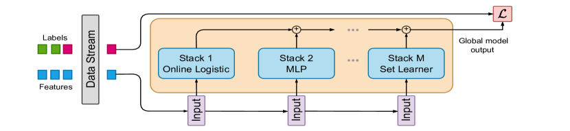
Figure 1: Multilearner Online Deep Learning. The dataset is streamed sequentially. Fast learners quickly adapt to the data distribution, providing a strong baseline for the deeper models. By synergizing models with different bias-variance trade-offs, the overall architecture can quickly adapt to the data and eventually learn deep representations.

Our proposed architecture is a result of three core elements in our design philosophy. First, different datasets are best treated by different model architectures. A true foundational model for online learning needs to adaptively select the architecture best suited for a task as it is training. This solves the shallow/deep model dilemma, as during different stages of training, the model can be guided more by shallow or deep models. Second, the base architecture should be simple and modular, so that different types of networks/layers can be incorporated. This allows a smooth transition, as more data become available, from relying predominantly on simple, learning-efficient models to focusing on more complex, highly expressive models. Third, the overall architecture needs to be efficient and minimize time complexity.

The main drawback of neural networks in the online setting is their sensitivity to hyperparameters. Deep neural networks require low learning rates to be stable during training, but this entails overfitting and accumulating large errors for millions of optimization steps. On the other hand, fast learners are typically shallow and train quicker, but lack the ability to learn complex representations. For example, it can be very difficult to know the optimal width or learning rate of the network before the dataset has been streamed. To address this challenge we propose the learning architecture depicted in Figure 1. Here the base fast learner based on online logistic regression quickly learns the linear approximation to the solution and provides the strongest signal guiding the global model output initially. As more data arrive, the second stage learner, implemented as an MLP, kicks in, providing only the delta on top of the online logistic regression baseline. Finally, the Set Learner, which has a deep structure and the ability to represent the semantics of variables, provides the modeling output that is the finest and therefore the hardest to learn. For example, learning semantic embeddings of variable IDs may take a long time, but this endows this part of the architecture with the ability to handle missing data and encode complex input-output relationships. Of course, this can be generalized beyond the three aforementioned learning levels. We choose to outline the structure used in our experiments, which also happens to capture the most important methodological thinking behind our approach. It is also important to note that since the task of the more complex learners is only to provide the delta on top of faster learners that train faster, they are much less sensitive to hyper-parameter selection.

Fast Learner. Consider the standard task of fitting a logistic regression model. Denote the dataset by $\mathcal{A}=\{(\mathbf{x}_{i},y_{i})\}_{i=1}^{n}$, with $\mathbf{x}\in\mathbb{R}^{m},y_{i}\in\{0,1\}$. For a simple generalized linear model $p(y|\mathbf{x},\theta)=\sigma(\mathbf{x}\theta)$, with weights $\theta\in\mathbb{R}^{m}$, where $\sigma(\cdot)$ is the logistic function, we assign a normal prior $p(\theta)=\mathcal{N}(\theta;\mathbf{m}_{0},\mathbf{P}_{0})$, with mean $\mathbf{m}_{0}\in\mathbb{R}^{m}$ and symmetric positive definite covariance matrix $\mathbf{P}_{0}\in\mathbb{R}^{m\times m}$.

Proposition 2.

Assuming an input feature distribution for $\mathbf{x}$ that is approximately normal, and linearizing the non-linear relationship, $\mathbf{y}=\sigma(\theta\mathbf{x})$, a quadratic approximation to the posterior of model weights after observing the $n$-th datapoint is given by the recursive formula $p(\theta|\{(\mathbf{x}_{i},y_{i})\}_{i=1}^{n})\approx\mathcal{N}(\theta;\mathbf{m}_{n},\mathbf{P}_{n})$, where:

$$\mathbf{m}_{n} =\mathbf{m}_{n-1}+\frac{\mathbf{P}_{n-1}\mathbf{x}_{n}^{\top}\left(1-\mathbf{\sigma}(\mathbf{x}_{n}\mathbf{m}_{n-1})\right)\sigma\left(\mathbf{x}_{n}\mathbf{m}_{n-1}\right)[\mathbf{y}_{n}-\sigma\left(\mathbf{x}_{n}\mathbf{m}_{n-1}\right)]}{\mathbf{x}_{n}\mathbf{P}_{n-1}\mathbf{x}_{n}^{\top}+\mathbf{P}_{n-1}\left[\left(1-\mathbf{\sigma}(\mathbf{x}_{n}\mathbf{m}_{n-1})\right)\sigma\left(\mathbf{x}_{n}\mathbf{m}_{n-1}\right)\right]^{2}},$$ (8)

$$\mathbf{P}_{n} =\mathbf{P}_{n-1}-\frac{\mathbf{P}_{n-1}\mathbf{x}_{n}^{\top}\mathbf{x}_{n}\mathbf{P}_{n-1}^{\top}\left[\left(1-\mathbf{\sigma}(\mathbf{x}_{n}\mathbf{m}_{n-1})\right)\sigma\left(\mathbf{x}_{n}\mathbf{m}_{n-1}\right)\right]^{2}}{\mathbf{x}_{n}\mathbf{P}_{n-1}\mathbf{x}_{n}^{\top}+\mathbf{P}_{n-1}\left[\left(1-\mathbf{\sigma}(\mathbf{x}_{n}\mathbf{m}_{n-1})\right)\sigma\left(\mathbf{x}_{n}\mathbf{m}_{n-1}\right)\right]^{2}}.$$ (9)

Proof.

The proof is in Appendix G. ∎

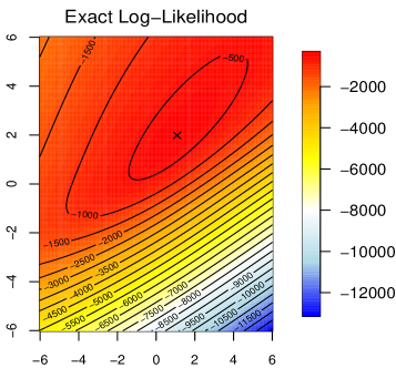
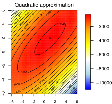
Figure 2: Exact log-likelihood vs. our proposed quadratic approximation. We see that close to the data-generating parameters (marked as x) both our approximation and the exact log-likelihood function agree. See Section G.3 for toy dataset experiment details.

Algorithm 2 Online Memoryless Bayesian Logistic Regression

Dataset $\mathcal{A}=\{(\mathbf{x}_{i},y_{i})\}_{i=1}^{n}$

Initialize: $p(\theta)=\mathcal{N}(\theta;\mathbf{m}_{0},\mathbf{P}_{0})$, $\mathbf{m}_{0}=0$, where $\mathbf{P_{0}}=\mathbf{I}$

Return $p(\theta|\{(\mathbf{x}_{i},y_{i})\}_{i=1}^{n})=\mathcal{N}(\theta;\mathbf{m}_{n},\mathbf{P}_{n})$

for t = 1,…,n do

     Receive instance: $\mathbf{x}_{t}$ and predict: $\hat{y}_{t}=\sigma(\mathbf{x}_{t}\mathbf{m}_{t-1})$

     Reveal true value: $y_{t}$ and update parameters:

$$S_{t} =\mathbf{x}_{t}\mathbf{P}_{t-1}\mathbf{x}_{t}^{\top}+\mathbf{P}\left[\left(1-\mathbf{\sigma}(\mathbf{x}_{t}\mathbf{m}_{t-1})\right)\sigma\left(\mathbf{x}_{t}\mathbf{m}_{t-1}\right)\right]^{2},$$ (10)

$$\mathbf{K}_{t} =\mathbf{P}_{t-1}\mathbf{X}_{t}^{\top}\left(1-\mathbf{\sigma}(\mathbf{x}_{t}\mathbf{m}_{t-1})\right)\sigma\left(\mathbf{x}_{t}\mathbf{m}_{t-1}\right)S_{t}^{-1},$$ (11)

$$\mathbf{m}_{t} =\mathbf{m}_{t-1}+\mathbf{K}_{t}[\mathbf{y}_{t}-\sigma\left(\mathbf{x}_{t}\mathbf{m}_{t-1}\right)],$$ (12)

$$\mathbf{P}_{t} =\mathbf{P}_{t-1}-\mathbf{K}_{t}S_{t}\mathbf{K}_{t}^{\top}.$$ (13)

end for

As a consequence of this recursive formula, we derive the sequential Algorithm 2, based on the quadratic approximation to the log-likelihood. This algorithm can process the dataset in one pass, while never storing any data in memory. The approximation is demonstrated in Figure 2, showing that it is accurate close to the maximizer of the exact log-likelihood. Note that $S_{t}^{-1}$ in Algorithm 2 is a scalar, so there is no need to invert any matrices in our approach. The only memory requirement is storage of the parameters of the normal posterior distribution. The parameters update proportionally to the “innovation” (eq. 12), which is data dependent, rather than set by the user. This fast learner is a high bias and low variance model. In the next section, we propose a highly expressive module that lies at the opposite end of the bias-variance spectrum.

Slow learner with set inputs. Rather than masking missing features with a zero or using deterministic dropout, as is done in (Agarwal et al., 2023), we treat the input as a set that excludes any missing features. Recall that the data generating process produces a sequence of triplets $\mathcal{P}=\{(\mathbf{z}_{1},\mathbf{y}_{1},\bm{\Omega}_{1}),\dots,(\mathbf{z}_{T},\mathbf{y}_{T},\bm{\Omega}_{T})\}$. Then, the set of input features $\mathcal{X}_{t}$ can be expressed as:

$$\mathcal{X}_{t} =\left\{\mathbf{z}_{t,j}:\bm{\Omega}_{t,j}=1\right\},\quad\mathcal{I}_{t}=\left\{j:\bm{\Omega}_{t,j}=1\right\},\quad\mathcal{D}=\left[(\mathcal{X}_{1},\mathcal{I}_{1},\mathbf{y}_{1}),\dots,(\mathcal{X}_{T},\mathcal{I}_{T},\mathbf{y}_{T})\right].$$ (14)

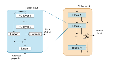
Figure 4: Visualization of our set learning decoder.

The size of the input feature set $\mathcal{X}_{t}$ is time varying. To allow the model to determine which inputs are available, it is necessary to pass a set of feature IDs in an index set $\mathcal{I}_{t}$. Our proposed set learning module follows closely the ProtoRes architecture (please refer to Oreshkin et al. (2022) for details). It takes the index set $\mathcal{I}_{t}$ and maps each of its active index positions to a continuous representation to create feature ID embeddings. It then concatenates each ID embedding to the corresponding feature value of $\mathcal{X}_{t}$. These feature values and ID embedding pairs are aggregated and summed to produce fixed dimensional vector representations that we denote as $\mathbf{x}_{0}$. The main components of our proposed set learning module are blocks, each consisting of $L$ fully connected (FC) layers. Residual skip connections are included in the architecture so that blocks can be bypassed. An input set $\mathcal{X}$ is mapped to $\mathbf{x}_{0}=\textsc{EMB}(\mathcal{X})$. The overall structure of the module at block $r\in\{1,\dots,R\}$ (see Fig. 4) is:

$$\mathbf{h}_{r,1} =\textsc{FC}_{r,1}(\mathbf{x}_{r-1}),\quad\dots,\quad\mathbf{h}_{r,L}=\textsc{FC}_{r,L}(\mathbf{h}_{r,L-1}),$$ (15)

$$\mathbf{x}_{r} =\textsc{ReLU}(\mathbf{W}_{r}\mathbf{x}_{r-1}+\mathbf{h}_{r-1,L})\,,\quad\hat{\mathbf{y}}_{r}=\hat{\mathbf{y}}_{r-1}+\mathbf{Q}_{L}\mathbf{h}_{r,L},$$ (16)

where $\mathbf{W}_{r},\mathbf{Q}_{L}$ are learnable matrices. We connect $R$ blocks sequentially to obtain global output $\hat{\mathbf{y}}_{R}$.

4.3 Combining the learners

There are many options for combining the learners. We considered three candidate choices. First, an intuitive approach is to consider the relative performance of the models in the data seen so far. For example, in a classification task, in order to merge the model predictions we may take a weighted combination by weighting each classifier proportionally to its accuracy rate. This approach conceptually mirrors the existing ODL approach, albeit using $\alpha$ values derived directly from past prediction performance, as opposed to learning them via hedge backpropagation as in Algorithm 1. Another approach is to combine the classifiers by multiplying their class probabilities (or summing the logarithm of the logits for better numerical stability). This approach can be theoretically interpreted as a joint predictive distribution across multiple independent predictors’ posteriors. Finally, we explore the simple approach of summing raw model outputs. Empirically this works surprisingly well and strongly outperforms model ensembling, for example (see Tab. 3). Furthermore, our experiments imply that this is due to the fast and weak models learning to synergize as they are co-trained. The strong learners receive strong baseline predictions that they build on top of and refine rather than trying to make a prediction from scratch. Our architecture is summarized in Figure 1.

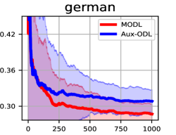
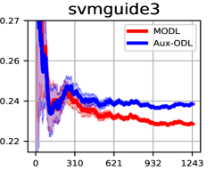
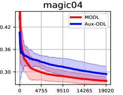
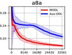
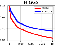
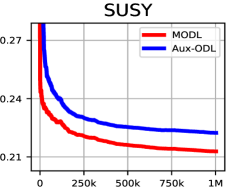
Figure 3: Comparison of normalized online error for ODL (with Aux-Drop) vs. our proposed model MODL on standard benchmarks. Shaded regions indicate 95% C.I. over multiple trials.

5 Empirical Results

Our experiments provide empirical support to the following: (i) our online learning model MODL consistently outperforms state-of-the-art online deep learning methods; (ii) new proposed modules, including the online logistic regression as well as the set learning component, work synergistically within the MODL framework; (iii) combining the modules is best done via summation, compared to a few alternatives, such as a mixture of experts, for example; (iv) the Fast ODL optimization framework is significantly more efficient than hedge backpropagation.

Datasets. We use common online deep learning datasets and replicate the setup from the prior work by Agarwal et al. (2023). Our results are based on 6 datasets of varying sizes. As stated in the review section, particle physics colliders produce enormous amounts of data which can require learning from a stream. For this reason we select two large particle physics datasets, HIGGS and SUSY (Baldi et al., 2014). HIGGS captures the process of the detection of the HIGGS boson during a particle accelerator experiment. SUSY is a dataset relating to the detection of SUper SYmmetric (SUSY) particles. Similar to HIGGS, the goal is to distinguish between measurements caused by a background noise process and the signal produced by the elusive super symmetric particles that are notoriously difficult to detect. We also test our model on german (Chang and Lin, 2011), a financial dataset where the goal is to identify consumer credit risk. Svmguide3 (Dua et al., 2017) is a synthetic binary classification dataset. Another physics dataset, magic04 (Chang and Lin, 2011), detects the presence of gamma particle radiation in Cherenkov telescope images. Finally, a8a (Dua et al., 2017) compiles census data with the task of predicting individuals with high incomes based on demographic information. More details about the datasets can be found in Appendix C.

Training Methodology. We closely follow the experimental setup of Aux-Drop (Agarwal et al., 2023). For small and medium datasets we run 20 independent trials, whereas for the large datasets we run 5. The random input masks for missing features and network initializations are from the same seed to ensure fairness. For all methods at each training step we process a single instance, so the batch size is fixed to 1. Additionally, since in learning from data streams it is not feasible to segregate the data into training, validation and test sets we report the results for basic hyperparameters and check how sensitive each approach is to the hyperparameters chosen which can be found in Section B.4. For missing feature experiments we randomly mask all features with some probability (except for the first two features that are always available). Note that this is done to replicate the setting of prior work for the purpose of comparing the algorithms; our algorithm does not require any features to be always available. For a detailed description of the hyperparameters, see Supplementary D.

Table 1: Comparison on standard datasets: cumulative error (mean $\pm$ st. deviation) over 20 runs. Each feature is present with probability $p_{\textrm{f}}$ (independently of other features and time).

Dataset	OLVF	Aux-Drop(ODL)	Aux-Drop(OGD)	MODL (ours)	$p_{\textrm{f}}$
german	333.4$\pm$9.7	306.6 $\pm$ 9.1	327.0$\pm$45.8	286 $\pm$ 5.3	0.73
svmguide3	346.4$\pm$11.6	296.9$\pm$1.3	296.6$\pm$0.6	288 $\pm$ 1.0	0.72
magic04	6152.4$\pm$54.7	5607.15 $\pm$ 235.1	5477.45 $\pm$ 299.3	5124 $\pm$ 153	0.68
a8a	8993.8$\pm$40.3	6700.4$\pm$124.5	7261.8$\pm$283.5	5670 $\pm$ 278	0.75

Table 2: Comparison on HIGGS and SUSY for various feature probabilities $p_{\textrm{f}}$. The metric is the mean ($\pm$ standard deviation) cumulative error in thousands over 5 runs.

$p_{\textrm{f}}$	HIGGS
	AuxDrop (ODL)	MODL (ours)
.01	440.2 $\pm$ 0.1	439.6 $\pm$ 0.1
.20	438.4 $\pm$ 0.1	435.6 $\pm$ 0.4
.50	427.4 $\pm$ 0.7	422.7 $\pm$ 0.3
.80	411.8 $\pm$ 0.4	399.6 $\pm$ 0.2
.95	399.4 $\pm$ 1.0	377.1 $\pm$ 0.5
.99	392.0 $\pm$ 1.0	366.4 $\pm$ 0.5

$p_{\textrm{f}}$	SUSY
	AuxDrop (ODL)	MODL (ours)
.01	285.0 $\pm$ 0.1	283.0 $\pm$ 0.1
.20	274.8 $\pm$ 0.9	271.8 $\pm$ 0.1
.50	256.6 $\pm$ 1.0	252.0 $\pm$ 0.1
.80	237.0 $\pm$ 0.7	230.6 $\pm$ 0.1
.95	226.2 $\pm$ 0.4	217.5 $\pm$ 0.1
.99	222.3 $\pm$ 0.2	212.2 $\pm$ 0.2

Key Results. Figure 3 shows that during training MODL remains consistently ahead of the current state-of-the-art model Aux-ODL with respect to the classification error rate. Besides converging faster, our approach also achieves a lower overall error rate at the end of training. These findings are replicated across datasets that vary in size over 3 orders of magnitude and with different feature missingness levels. The detailed results for the cumulative miss-classification metric are summarized in Tables 1 and 2. For the small and medium datasets shown in Table 1 we can see that MODL is the clear top performer, reducing error on average by 11%. We note that the improvements are measured over 20 trials and are all statistically significant at the 0.05 level using a paired Wilcoxon test. For the large datasets in Table 6 we conduct a detailed feature missingness experiment for 13 different noise levels with 5 trials per level. The results show that MODL is consistently improving the state-of-the-art for all noise levels. This is an important result as it verifies the strength of our approach for a wide spectrum of feature noise, ranging from near-zero up to extreme levels of noise.

The efficiency of the Fast ODL optimization scheme described in Section 4.1 is empirically verified to correspond to the expected theoretical time complexity in Table 5. For this experiment we employ the standard ODL algorithm and vary the number of layers and the embedding size. We see that in all cases our proposed optimization called “Fast ODL” reduces the the training time dramatically, e.g., from 63 hours to 9.

Ablation Studies. In this section we rigorously verify our model components. Specifically, we look at the impact of removing on or more modules of our architecture. Table 4 shows that removing any individual component negatively affects the overall performance. From these results we ascertain that the presence of diverse learners with respect to the bias-variance trade-off bolsters performance.

The second ablation experiment explores different ways to merge learner predictions. MODL merges predictions by direct summation of the constituent learners. We consider alternative approaches that incude: (i) learnable gating functions in a Mixture of Experts (MoE) style setup where the final output is a weighted sum of each learner’s prediction; (ii) multiplying the logit probabilities (by summing the logarithm of the predicted logits); and (iii) a greedy weighting scheme that assigns more weight to learners with higher running accuracy.

A particularly challenging and sensitive hyperparameter to select in online learning is the learning rate. We run sensitivity experiments with respect to the learning rate in the large bennchmarks. Our results in LABEL:tab:lr_study show increased robustness to learning rate selection. This is expected because our framework incorporates learners that train without backpropagation, which safeguards against selecting learning rates that are far from optimal.

Table 3: Ablation study on merging constituent learner outputs HIGGS ($p_{\textrm{f}}$=0.5), SUSY ($p_{\textrm{f}}$=0.99).

Dataset	Soft rel. error	Mult.	Ensemble	Mix. of Experts	Sum (ours)
german	293.0$\pm$10.3	294.9$\pm$7.1	307.5$\pm$21.0	316.2$\pm$9.3	285.9$\pm$7.2
svmguide3	296.3$\pm$1.5	299.5$\pm$6.5	296.6$\pm$1.5	298.4$\pm$3.3	287.5$\pm$4.0
magic04	4720$\pm$154	5146$\pm$75	6506$\pm$ 588	6719$\pm$44	5226 $\pm$ 98
a8a	6495$\pm$709	5691$\pm$40	5865$\pm$40	6190$\pm$168	5673$\pm$36
HIGGS	442.8$\pm$0.3k	422.7$\pm$0.6k	428.8$\pm$0.1k	431.9$\pm$0.9k	422.7$\pm$0.3k
SUSY	220.2$\pm$0.8k	212.3$\pm$0.1k	218.7$\pm$0.2k	217.0$\pm$0.2k	212.2$\pm$0.2k

Table 4: Ablation of proposed model components. We show that for each learner that we add the overall model performance improves.

$p_{\textrm{f}}$	HIGGS			SUSY
	OL + MLP	OL + Set	MODL (ours)	OL + MLP	OL + Set	MODL (ours)
.01	442.7$\pm$0.2	450.2$\pm$0.4	439.6 $\pm$ 0.1	285.3$\pm$0.1	332.6$\pm$0.3	283.0 $\pm$ 0.1
.20	439.9$\pm$0.1	450.3$\pm$0.2	435.6 $\pm$ 0.4	274.0$\pm$0.1	352.4$\pm$0.3	271.8 $\pm$ 0.1
.50	430.3$\pm$0.2	450.1$\pm$0.1	422.8 $\pm$ 0.3	255.0$\pm$0.1	343.3$\pm$0.6	252.0 $\pm$ 0.1
.80	411.7$\pm$0.1	449.6$\pm$0.2	399.6 $\pm$ 0.2	234.3$\pm$0.1	326.3$\pm$0.4	230.6 $\pm$ 0.1
.95	394.1$\pm$0.5	448.5$\pm$0.1	377.1 $\pm$ 0.5	222.1$\pm$0.1	320.9$\pm$0.4	217.5 $\pm$ 0.1
.99	386.6$\pm$0.1	447.1$\pm$0.1	366.4 $\pm$ 0.6	217.3$\pm$0.1	316.3$\pm$0.6	212.2 $\pm$ 0.2

Table 5: Comparison in hours between Aux-Drop (ODL) and Fast ODL on HIGGS for $p_{\mathbf{f}}=0.5$ with 20 layers and embedding dim. $E$. We massively speed up training while maintaining performance.

Experiment	ODL (AuxDrop)	Fast ODL (AuxDrop)	Time ODL vs. Fast ODL
HIGGS ($E=25$)	431.4 $\pm$ 0.5	431.0 $\pm$ 0.5	57:04:12 vs. 9:23:13
HIGGS ($E=50$)	429.2 $\pm$ 0.4	429.4 $\pm$ 0.4	54:04:10 vs. 8:43:11
HIGGS ($E=100$)	427.6 $\pm$ 0.5	427.8 $\pm$ 0.5	63:19:05 vs. 8:58:51

6 Conclusion

Limitations. Our work is focused on supervised learning from streams of data. This is not trivially applicable to other areas such as online reinforcement learning. While our work shows that including multiple learners with different bias-variance trade-offs is a sensible approach to online deep learning, it does not show how many learners, and which types, are necessary to achieve specific error bounds. Although MODL works in a general multi-class setting our experiments focused on binary tasks. This limitation applies to all standard methods in our area (Sahoo et al., 2018; Agarwal et al., 2023).

Overview. We demonstrate that the problem of online deep learning is best handled synergistically by multiple learners that operate at various points of the convergence speed/expressivity trade-off curve. We derive a very fast learning and non-backpropagation based approach to support early stages of learning and to provide a strong baseline for other learners. Then, at the other end of the spectrum, we propose a slowly learning, yet very expressive set learner that is invariant to feature ordering and robust to missing features. When appropriately combined, these approaches significantly improve performance while reducing training complexity.

MODL: Multilearner Online Deep Learning
Supplementary material

Appendix A Broader Impact Statement

Our paper introduces a new Online Learning technique and improves existing training methodologies for online learning of deep neural networks. We show that co-training multiple learners can lead to significantly faster convergence as well as improved overall model performance at inference time.

A strongly positive outcome stemming from our contributions is the significant reduction of training time from quadratic complexity in network parameters down to linear complexity. This has profound consequences for training deep models online as it significantly decreases the necessary training compute. Thus the energy spent for training deep online learners is massively reduced.

Furthermore, the improved convergence speed and overall performance of our proposed technique MODL means that our model is more data efficient than existing ones leading to a moderately reduced need for large dataset sizes. Efficiently learning in one pass means that data does not need to be stored which strongly protects the privacy rights of individuals and organizations. Training online, i.e., without storing data can help companies comply with data protection laws and can allow the consumer to have greater confidence that their fundamental human right of privacy is protected.

Nevertheless, as with all methods in machine learning there are broader impact concerns with our work. Our proposed methods are by no means immune to dataset bias; a well documented problem. Risk mitigation mechanisms include A.I. fairness research techniques that broadly apply to neural networks as well as model intrepretability. In our case is the potential to interpret model outputs is particularly strong for the weaker learners such as logistic regression.

We are confident that our research effort offers more benefits in energy saving and data privacy as opposed to the risks posed by the usage of deep models that are prone to bias in the data. Furthmore, we point out that the risks posed by a potential deployment of our model can be hedged against due to the interpretability of some of our constituent learners.

Appendix B Additional Experiments

B.1 Feature Missingness Experiment

In this section we provide additional experiments in support of the summary results presented in the main text. More concretely, we provide a full feature missningess study with 13 unique $p_{\textbf{f}}$ values for the large benchmarks HIGGS and SUSY. As shown in Tab. 6, our model convincingly outperforms in all settings. We observe that the advantage of our method increases as more features become available.

Table 6: Comparison on HIGGS and SUSY for various feature probabilities $p_{\textrm{f}}$. The metric is the mean ($\pm$ standard deviation) cumulative error in thousands (5 runs).

$p_{\textrm{f}}$	HIGGS
	AuxDrop (ODL)	MODL (ours)
.01	440.2 $\pm$ 0.1	439.6 $\pm$ 0.1
.05	440.0 $\pm$ 0.1	439.5 $\pm$ 0.2
.10	440.0 $\pm$ 0.2	438.5 $\pm$ 0.1
.20	438.4 $\pm$ 0.1	435.6 $\pm$ 0.4
.30	435.1 $\pm$ 0.2	432.3 $\pm$ 0.3
.40	432.0 $\pm$ 0.3	428.4 $\pm$ 0.3
.50	427.4 $\pm$ 0.7	422.8 $\pm$ 0.4
.60	423.2 $\pm$ 0.5	422.8 $\pm$ 0.2
.70	418.5 $\pm$ 0.7	409.5 $\pm$ 0.4
.80	411.8 $\pm$ 0.4	399.6 $\pm$ 0.3
.90	405.6 $\pm$ 0.7	387.0 $\pm$ 0.3
.95	399.4 $\pm$ 1.0	377.2 $\pm$ 0.5
.99	392.1 $\pm$ 1.0	366.5 $\pm$ 0.6

$p_{\textrm{f}}$	SUSY
	AuxDrop (ODL)	MODL (ours)
.01	285.0 $\pm$ 0.1	283.0 $\pm$ 0.1
.05	283.3 $\pm$ 0.2	281.0 $\pm$ 0.1
.10	280.6 $\pm$ 0.5	278.0 $\pm$ 0.1
.20	274.9 $\pm$ 0.9	271.9 $\pm$ 0.1
.30	269.0 $\pm$ 0.7	265.5 $\pm$ 0.1
.40	262.8 $\pm$ 0.9	258.9 $\pm$ 0.1
.50	256.7 $\pm$ 1.0	252.0 $\pm$ 0.1
.60	250.0 $\pm$ 0.9	244.7 $\pm$ 0.2
.70	243.9 $\pm$ 0.7	238.0 $\pm$ 0.2
.80	237.0 $\pm$ 0.7	230.6 $\pm$ 0.1
.90	230.0 $\pm$ 0.7	222.3 $\pm$ 0.2
.95	226.2 $\pm$ 0.4	217.5 $\pm$ 0.1
.99	222.2 $\pm$ 0.2	212.2 $\pm$ 0.2

B.2 Model Ablation Study

In this section we empirically validate our proposed model MODL. As shown in Tab 7 the results in the main paper persist in the additional feature missningness settings further validating our conclusion that all of our model components are necessary.

Table 7: Ablation of proposed model components. We show that for each learner that we add the overall model performance improves.

$p_{\textrm{f}}$	HIGGS			SUSY
	OL + MLP	OL + Set Learner	MODL (ours)	OL + MLP	OL + Set Learner	MODL (ours)
.01	442.8$\pm$0.2	450.2$\pm$0.5	439.6 $\pm$ 0.1	285.3$\pm$0.1	332.6$\pm$2.1	283.0 $\pm$ 0.1
.05	442.7$\pm$0.1	449.9$\pm$0.4	439.5 $\pm$ 0.2	283.3$\pm$0.1	334.7$\pm$1.9	281.1 $\pm$ 0.1
.10	441.9$\pm$0.1	450.1$\pm$0.3	438.5 $\pm$ 0.1	280.0$\pm$0.1	337.8$\pm$1.4	278.0 $\pm$ 0.1
.20	439.9$\pm$0.1	450.3$\pm$0.2	435.6 $\pm$ 0.4	274.0$\pm$0.1	352.4$\pm$0.3	271.9 $\pm$ 0.1
.30	437.4$\pm$0.1	450.1$\pm$0.3	432.3 $\pm$ 0.3	267.9$\pm$0.1	355.4$\pm$0.3	265.5 $\pm$ 0.1
.40	434.9$\pm$332	450.3$\pm$404	428.4 $\pm$ 302	261.7$\pm$0.1	338.9$\pm$0.4	258.9 $\pm$ 0.1
.50	430.3$\pm$193	450.1$\pm$93	422.8 $\pm$ 386	255.0$\pm$0.1	343.3$\pm$0.7	252.0 $\pm$ 0.1
.60	425.4$\pm$178	449.9$\pm$137	422.8 $\pm$ 244	248.3$\pm$0.1	336.6$\pm$0.5	244.7 $\pm$ 0.2
.70	420.5$\pm$484	451.0$\pm$122	409.5 $\pm$ 424	241.3$\pm$0.1	337.9$\pm$0.4	238.0 $\pm$ 0.1
.80	411.8$\pm$106	449.6$\pm$219	399.6 $\pm$ 256	234.3$\pm$0.1	326.3$\pm$0.4	230.6 $\pm$ 0.1
.90	401.4$\pm$517	449.8$\pm$58	387.0 $\pm$ 348	226.5$\pm$0.2	322.0$\pm$0.4	222.3 $\pm$ 0.2
.95	394.1$\pm$565	448.5$\pm$175	377.2 $\pm$ 537	222.1$\pm$0.1	320.9$\pm$0.4	217.5 $\pm$ 0.1
.99	386.7$\pm$133	447.1$\pm$163	366.4 $\pm$ 588	217.4$\pm$0.1	316.4$\pm$0.7	212.2 $\pm$ 0.2

B.3 Training Time Additional Settings

In this section we explore the wall clock training time reduction offered by our proposed fast training scheme on large datasetrs. We note that the training time savings range from 30% to over 80%!

Table 8: Time comparison between AuxDropODL and FastAuxDropODL on HIGGS and SUSY for $p=0.5$ (various layer and embedding dimensions).

Experiment	Aux-ODL	Fast Aux-(FODL)	Time ODL vs. FODL
HIGGS ($L=5,E=25$)	431.9 $\pm$ 0.5	431.4 $\pm$ 0.5	5:35:10 vs. 3:34:55
HIGGS ($L=5,E=50$)	429.6 $\pm$ 0.5	429.6 $\pm$ 0.6	5:41:05 vs. 3:38:18
HIGGS ($L=5,E=100$)	428.0 $\pm$ 0.3	427.9 $\pm$ 0.3	5:45:56 vs. 3:38:42
HIGGS ($L=11,E=25$)	429.8 $\pm$ 0.7	429.7 $\pm$ 0.4	22:44:06 vs. 6:21:58
HIGGS ($L=11,E=50$)	427.4 $\pm$ 0.5	427.4 $\pm$ 0.7	16:04:59 vs. 4:29:05
HIGGS ($L=11,E=100$)	426.9 $\pm$ 0.3	426.6 $\pm$ 0.3	20:05:39 vs. 6:32:20
HIGGS ($L=20,E=25$)	431.4 $\pm$ 0.5	431.0 $\pm$ 0.5	57:04:12 vs. 9:23:13
HIGGS ($L=20,E=50$)	429.2 $\pm$ 0.4	429.4 $\pm$ 0.4	54:04:10 vs. 8:43:11
HIGGS ($L=20,E=100$)	427.6 $\pm$ 0.5	427.8 $\pm$ 0.4	63:19:05 vs. 8:58:51
SUSY ($L=5,E=25$)	257.3 $\pm$ 1.0	257.3 $\pm$ 1.2	5:33:53 vs. 2:59:32
SUSY ($L=5,E=50$)	256.6 $\pm$ 0.9	256.6 $\pm$ 0.9	5:37:42 vs. 3:03:09
SUSY ($L=5,E=100$)	255.9 $\pm$ 0.4	255.8 $\pm$ 0.5	5:07:21 vs. 3:41:03
SUSY ($L=11,E=25$)	257.2 $\pm$ 0.9	257.5 $\pm$ 1.1	22:41:05 vs. 6:19:03
SUSY ($L=11,E=50$)	257.0 $\pm$ 1.2	256.7 $\pm$ 1.0	23:04:11 vs. 6:54:21
SUSY ($L=11,E=100$)	255.9 $\pm$ 0.8	256.1 $\pm$ 0.8	20:05:06 vs. 6:29:58
SUSY ($L=20,E=25$)	258.6 $\pm$ 1.1	258.5 $\pm$ 1.3	36:39:13 vs. 8:44:24
SUSY ($L=20,E=50$)	257.4 $\pm$ 0.9	257.4 $\pm$ 0.9	39:59:38 vs. 8:01:53
SUSY ($L=20,E=100$)	257.3 $\pm$ 1.0	257.1 $\pm$ 1.0	43:07:45 vs. 8:19:44

B.4 Learning Rate Sensitivity Experiments

In this section we demonstrate that our model has stable and better performance than the baselines approach for a broad range of learning rates. This is due to the incorporation of learners without a backpropagation update which shields from but learning rate selections. Note that if we set the learning rate too high the other learners may become unstable so that protection from bad learning rates has reasonable limits (i.e. cannot train with absurd learning rates such as 0.5 with or higher). The conclusion from this section and Tab. LABEL:tab:lr_study is that for any reasonable learning rate selection for deep models our model outperforms.

Table 9: Error in HIGGS and SUSY for various learning rates with fixed probability of unreliable features $p_{f}=0.99$. The metric is reported as the mean $\pm$ standard deviation of the number of errors in 5 runs (11 layer Aux networks).

lr	HIGGS		SUSY
	AuxDrop (ODL)	MODL (ours)	AuxDrop (ODL)	MODL (ours)
0.00005	470.9$\pm$0.8	426.1$\pm$ 1.2	391.9 $\pm$ 67	225.5 $\pm$ 0.7
0.0001	470.1$\pm$0.7	415.4$\pm$0.8	333.4$\pm$62	222.2 $\pm$ 0.4
0.0005	442.8$\pm$3.5	392.7$\pm$0.6	278.6$\pm$21	216.6 $\pm$ 0.2
0.001	402.1$\pm$6.4	366.5$\pm$0.6	225.9$\pm$1.9	212.2 $\pm$ 0.2
0.005	439.4$\pm$11.4	383.3$\pm$0.9	253.6$\pm$11	215.0 $\pm$ 0.3
0.01	389.9$\pm$1.8	368.9$\pm$0.5	222.7$\pm$0.9	212.8 $\pm$ 0.1
0.05	392.1$\pm$0.8	421.1$\pm$0.5	222.4$\pm$0.2	227.2 $\pm$ 0.1
0.1	418.7$\pm$5.9	461.9$\pm$0.3	227.6$\pm$0.5	242.4 $\pm$ 0.4

Appendix C Dataset Statistics

Our dataset pre-processing follows exactly the steps from Agarwal et al. [2023]. The data is publicly available for download online. We provide summary dataset statistics in Tab. 10. The use of diverse dataset sizes aims to illustrate the strength of our approach in settings with low data (one thousand), moderate amount (tens of thousands) and large data (millions).

Table 10: Dataset statistics for the data used in our experiments.

Dataset	Size	Feature Size	Task
german	1000	24	Classification
svmguide3	1243	21	Classification
magic04	19020	10	Classification
a8a	32561	123	Classification
SUSY	1000000	8	Classification
HIGGS	1000000	21	Classification

Appendix D Hyperparameters and Computational Resources

D.1 Hyperparameters

Aux-ODL: We used the official repository of Aux-ODL with the tuned hyperparameters from the original paper by Agarwal et al. [2023] without makiung any changes. Namely, for the small datasets in our experiments we run 6-layer networks with learning rates 0.1 for german and svmguide3 and 0.01 for magic04 and a8a. For the large datasets, we used 11 layer networks with learning rate equal to 0.05. For all experiments we used the recommended layer size and AuxLayer dimension and position in the network. Additionally, the ODL discount rate was set to $\beta=0.99$ and the smoothing rate was set to $s=0.2$.

MODL: We used the exact same architecture in all experiments. Specifically, the online logistic regression learner is implemented identically for all datasets and the MLP has 3 hidden layers with 250 neurons. The set learner consists of 6 blocks with 3 layers per block. The width of each layer is set to 128 neurons. Our experiment code is publicly accessible.

D.2 Computational Resources

We run our experiments on a HP DL-580 Gen 7 server equipped with Intel Xeon E7-4870 2.40GHz 10-Core 30MB LGA1567 CPUs. In total we used 160 CPUs for our experiments. Note that using GPUs in the online learning setting is not effective as the batch size is 1. Therefore, given that our task is purely sequential we opt for a CPU server that is actually faster than a GPU server given the nature of the online learning task.

Appendix E Background

E.1 De Finetti Representation Theorem

For $n\geq 1$ the de Finetti representation for the joint mass or density of exchangeable discrete random variables $Y_{1},\dots,Y_{n}$ is given by

$$p_{Y_{1},\dots,Y_{n}}(y_{1},\dots,y_{n})=\int_{\Theta}\prod_{i=1}^{n}f_{Y}(y_{i};\theta)\pi_{0}(d\theta)$$

where $p_{Y}(y;\theta)$ is a mass function in $y$, and $\theta$ is a parameter lying in a space $\Theta\in\mathbb{R}^{p}$, for some (prior) distribution $\pi_{0}(d\theta)$ defined on $\theta$, where we may interpret $\Theta$ as the smallest set such that $\int_{\Theta}\pi_{0}(d\theta)=1.$ Using basic properties of probability we may derive an expression for the posterior predictive distribution for $Y_{n+1}$ (another element of the infinitely exchangeable sequence) conditional on $Y_{1}=y_{1},\dots,Y_{n}=y_{n}$. This defines the posterior density, $\pi_{n}(d\theta)$, as an updated version of $\pi_{0}(d\theta)$. We may re-write the postirior predictive using the definition of conditional probability as

$$p_{n}(y_{n+1})=\frac{p_{0}(y_{1},\cdots,y_{n},y_{n+1})}{p_{0}(y_{1},\cdots,y_{n})}=\int f_{Y}(y_{n+1};\theta)\pi_{n}(\theta)\,d\theta$$ (17)

where

$$\pi_{n}(\theta)=\frac{1}{p_{0}(y_{1},\cdots,y_{n})}\prod_{i=1}^{n}f(y_{i};\theta)\pi_{0}(\theta),$$ (18)

is the posterior. Note that this is the same form as the De Finetti representation with an updated version of $\pi_{0}$.

This result is important as it shows that the posterior predictive is the same whether we consider the initial prior and the likelihood of a full batch on $n$ observations or if we use an iterative update rule to modify the prior at each time step. Thus, we may simply update the prior for the $n+1$-th observation to be the posterior after the $n$-th observation without the need to maintain the any of the previous observations in memory. This allows us to derive recursive algorithms that update prior-posterior parameters without storing observations. Essentially, as long as we maintain a statistic that is sufficient in the Bayesian sense, the posterior distribution depends on the data only through the observed value of the statistic and the data may be discarded.

E.2 Bayesian Linear Regression

For a dataset $\mathcal{D}=\{(t_{1},y_{1}),\dots,(y_{N},t_{N})\}$, consider a classic regression model of the form:

$$y_{k}=\mathbf{x}_{k}\mathbf{\theta}+\varepsilon_{k},$$ (19)

where $y_{k}$ is a scalar outcome, $\mathbf{\theta}\in\mathbb{R}^{d\times 1}$ is the parameter of interest, $\mathbf{x}_{k}\in\mathbb{R}^{1\times d}$ is the feature vector and $\varepsilon_{k}\sim\mathcal{N}(0,\sigma^{2})$ is normally distributed noise. To simplify the notation we may stack all feature vectors in the designer matrix $\mathbf{X}\in\mathbb{R}^{N\times d}$ and the corresponding outcomes in a vector $\mathbf{y}_{k}\in\mathbb{R}^{N}$.

Though the problem can be solved in a purely least squares fashion or equivalently via maximum-likelihood approach we employ a standard Bayesian formulation. Assigning prior.

$$\pi_{0}(\mathbf{\theta})=\mathcal{N}(\mathbf{\theta}\,\lvert\,\mathbf{m}_{0},\mathbf{P}_{0})$$ (20)

for some $\mathbf{m}_{0}\in\mathbb{R}^{d},\mathbf{P}_{0}\in\mathbb{R}^{d\times d}$ and modeling $p(\mathbf{y}_{k}\,\lvert\,\mathbf{\theta})$ as

$$p(y_{k}\,\lvert\,\mathbf{\theta})=\mathcal{N}(y_{k}\,\lvert\,\mathbf{x}_{k}\mathbf{\theta},\sigma^{2}),$$ (21)

we may then apply Bayes rule to recover the posterior distribution over the parameter.

$$p(\theta\,\lvert\,y_{1:N}) \propto p(\theta)\prod_{k=1}^{N}p(y_{k}\,\lvert\,\theta)=\mathcal{N}(\mathbf{\theta}\,\lvert\,\mathbf{m}_{0},\mathbf{P}_{0})\prod_{k=1}^{N}\mathcal{N}(y_{k}\,\lvert\,\mathbf{x}_{k}\mathbf{\theta},\sigma^{2})$$ (22)

$$=\mathcal{N}(\mathbf{\theta}\,\lvert\,\mathbf{m}_{N},\mathbf{P}_{N}),$$ (23)

where the last equality follows by well known result Normal priors and Normal likelihoods yielding normal posteriors. In fact, it can be shown that

$$\mathbf{m}_{N} =\left[\mathbf{P}_{0}^{-1}+\frac{1}{\sigma^{2}}\mathbf{X}^{\top}\mathbf{X}\right]^{-1}\left[\frac{1}{\sigma^{2}}\mathbf{X}^{\top}\mathbf{y}+\mathbf{P}^{-1}_{0}\mathbf{m}_{0}\right],$$ (24)

$$\mathbf{P}_{N} =\left[\mathbf{P}_{0}^{-1}+\frac{1}{\sigma^{2}}\mathbf{X}^{\top}\mathbf{X}\right]^{-1}.$$ (25)

E.3 Online Bayesian Linear Regression

A disadvantage of full batch regression is that it requires keeping a large matrix $\left[\mathbf{P}_{0}^{-1}+\frac{1}{\sigma^{2}}\mathbf{X}^{\top}\mathbf{X}\right]^{-1}$ in memory and needing to invert it. To address these concerns we can use an efficient and recursive version of the algorithm. From the recursive de Finetti represention result we proved earlier we may alternatively calculate a posterior at step $n$-$1$ and treat it as a prior for step $n$.

$$p(\theta\,\lvert\,y_{1:n}) \propto p(\theta\,\lvert\,y_{1:n-1})p(y_{n}\,\lvert\,\theta)=\mathcal{N}(\mathbf{\theta}\,\lvert\,\mathbf{m}_{n-1},\mathbf{P}_{n-1})\mathcal{N}(y_{k}\,\lvert\,\mathbf{x}_{k}\mathbf{\theta},\sigma^{2})$$ (26)

$$=\mathcal{N}(\mathbf{\theta}\,\lvert\,\mathbf{m}_{n},\mathbf{P}_{n}),$$ (27)

where

$$\mathbf{m}_{n} =\left[\mathbf{P}_{n-1}^{-1}+\frac{1}{\sigma^{2}}\mathbf{X}_{n}^{\top}\mathbf{X}_{n}\right]^{-1}\left[\frac{1}{\sigma^{2}}\mathbf{X}_{n}^{\top}\mathbf{y}_{n}+\mathbf{P}_{n-1}^{-1}\mathbf{m}_{n-1}\right],$$ (28)

$$\mathbf{P}_{n} =\left[\mathbf{P}_{n-1}^{-1}+\frac{1}{\sigma^{2}}\mathbf{X}_{n}^{\top}\mathbf{X}_{n}\right]^{-1}.$$ (29)

In the above notation, $\mathbf{X}_{n}$ and $\mathbf{y}_{n}$ indicate that we take the $n$-th rows of $\mathbf{X}$, $\mathbf{y}$.

The matrix inversion lemma, also known as the Woodbury matrix identity.

$$\mathbf{P}_{n}=\left[\mathbf{P}_{n-1}^{-1}+\frac{1}{\sigma^{2}}\mathbf{X}_{n}^{\top}\mathbf{X}_{n}\right]^{-1}=\mathbf{P}_{n-1}-\mathbf{P}_{n-1}\mathbf{X}_{n}^{\top}\left[\mathbf{X}_{n}\mathbf{P}_{n-1}\mathbf{X}_{n}^{\top}+\sigma^{2}\right]^{-1}\mathbf{X}_{n}\mathbf{P}_{n-1}.$$ (30)

Note that the inverse term in the right hand side is a scalar and easy to compute.

The recursive set of equations takes the form:

$$S_{n} =\mathbf{X}_{n}\mathbf{P}_{n-1}\mathbf{X}_{n}^{\top}+\sigma^{2},$$ (31)

$$\mathbf{K}_{n} =\mathbf{P}_{n-1}\mathbf{X}_{n}^{\top}S_{n}^{-1},$$ (32)

$$\mathbf{m}_{n} =\mathbf{m}_{n-1}+\mathbf{K}_{n}[\mathbf{y}_{n}-\mathbf{X}_{n}\mathbf{m}_{n-1}],$$ (33)

$$\mathbf{P}_{n} =\mathbf{P}_{n-1}-\mathbf{K}_{n}S_{n}\mathbf{K}_{n}^{\top}.$$ (34)

Appendix F Logistic Regression

Consider a Generalized Linear Model (GLM) with link function $g(\cdot)=\text{logit}^{-1}(\cdot)$. For binary classification we define $p(y\,\lvert\,x)=\mathbb{E}_{Y|X}[y\,\lvert\,\mathbf{x}]=g^{-1}(\mathbf{x}\theta)=\sigma(\mathbf{x}\theta)=\mu$, $\sigma(\cdot)$ is the sigmoid function. The problem of finding the optimal parameter can be solved by maximizing the (log) likelihood numerically as it is convex. More precisely the derivative of the log-likelihood and the Hessian can be shown to be

$$\dot{\ell}_{n}(\theta)=\mathbf{X}^{\top}(\mathbf{y}-\bm{\mu}),$$ (35)

$$\ddot{\ell}_{n}(\theta)=-\mathbf{X}^{\top}\mathbf{D}\mathbf{X},$$ (36)

where $\bm{\mu}=[\sigma(\mathbf{X}_{1}\theta),\dots,\sigma(\mathbf{X}_{n}\theta)]$ is a vector containing the model prediction for each input, $\mathbf{D}$ is a diagonal matrix with the diagonal entries $[\sigma(\mathbf{X}_{1}\theta)(1-\sigma(\mathbf{X}_{1}\theta)),\dots,\sigma(\mathbf{X}_{n}\theta)(1-\sigma(\mathbf{X}_{n}\theta))].$ Note that since this is a convex problem so it has a unique solution that can be recovered via standard convex optimization techniques.

Appendix G Online Logistic Regression Derivation

G.1 Proof of Proposition 2

By standard random variable transformation theory we know that for invertible $h(\cdot):\mathbb{R}^{n}\to\mathbb{R}^{m}$ for $\mathbf{z}\in\mathbb{R}^{n}$ and $\mathbf{y}\in\mathbb{R}^{m}$ if

$$\mathbf{z}\sim\mathcal{N}(\mathbf{z}\,\lvert\,\mathbf{m},\mathbf{P})$$ (37)

$$\mathbf{y}=h(\mathbf{z})+\varepsilon_{t},$$ (38)

where we model the output as receiving additive noise $\varepsilon\sim\mathcal{N}(\varepsilon_{t}\,|\,0,\bm{\Sigma}_{t})$ independently from the input. then $p(\mathbf{y})=\mathcal{N}(h^{-1}(\mathbf{y})\,\lvert\,\mathbf{m},\mathbf{P})|\mathcal{J}(\mathbf{y})|^{-1}$, where $|\mathcal{J}(\mathbf{y})|$ is the Jacobian of $h$ evaluated at $\mathbf{y}$.

A challenge in analyzing this model is that it is non-linear. A standard technique to approximate $p(\mathbf{y})$ is to apply a first order Taylor approximation and linearize the function locally around the mean of the normal $\mathcal{N}(\mathbf{z}\,\lvert\,\mathbf{m},\mathbf{P})$ with some random perturbation $\delta\mathbf{z}\sim\mathcal{N}(\delta\mathbf{z}\,|\,0,\mathbf{P})$.

$$h(\mathbf{z})=g(\mathbf{m}+\delta\mathbf{z})\approx g(\mathbf{m})+\mathcal{J}(\mathbf{m})\delta\mathbf{z}=\widehat{h}(\mathbf{z}).$$ (39)

Firstly, note that $\mathbb{E}[h(\mathbf{z})]\approx\mathbb{E}[h(\mathbf{m})]+\mathcal{J(\mathbf{m})}\mathbb{E}[\delta\mathbf{z}]=\mathbb{E}[h(\mathbf{m})]$. Similarly, for the covariance matrix it follows that cov$(h(\mathbf{x}))=\mathbb{E}\left[(h(\mathbf{z})-\mathbb{E}[h(\mathbf{z})])(h(\mathbf{z})-\mathbb{E}[h(\mathbf{z})])^{\top}\right]\approx\mathcal{J}(\mathbf{m})\mathbf{P}\mathcal{J}(\mathbf{m})^{\top}.$ To show this in detail consider:

$$\text{cov}(h(\mathbf{z})) =\mathbb{E}\left[(h(\mathbf{z})-\mathbb{E}[h(\mathbf{z})])(h(\mathbf{z})-\mathbb{E}[h(\mathbf{z})])^{\top}\right]$$ (40)

$$\approx\mathbb{E}\left[(h(\mathbf{z})-h(\mathbf{m}))(h(\mathbf{z})-h(\mathbf{m}))^{\top}\right]$$ (41)

$$=\mathbb{E}\left[(h(\mathbf{m})+\mathcal{J}(\mathbf{m})\delta\mathbf{z}-h(\mathbf{m}))(h(\mathbf{m})+\mathcal{J}(\mathbf{m})\delta\mathbf{z}-h(\mathbf{m}))^{\top}\right]$$ (42)

$$=\mathbb{E}\left[(\mathcal{J}(\mathbf{m})\delta\mathbf{z})(\mathcal{J}(\mathbf{m})\delta\mathbf{z})^{\top}\right]$$ (43)

$$=\mathcal{J}(\mathbf{m})\mathbb{E}\left[(\delta\mathbf{z})(\delta\mathbf{z})^{\top}\right]\mathcal{J}(\mathbf{m})^{\top}$$ (44)

$$=\mathcal{J}(\mathbf{m})\mathbf{P}\mathcal{J}(\mathbf{m})^{\top}.$$ (45)

Combining the previous results we obtain an approximate joint distribution of $\mathbf{z},\mathbf{h}(\mathbf{z})$:

$$p\left(\begin{bmatrix}\mathbf{z}\\ \mathbf{y}\end{bmatrix}\right)=\mathcal{N}\left(\begin{bmatrix}\mathbf{m}\\ h(\mathbf{m})\end{bmatrix},\begin{bmatrix}\mathbf{P}&[\mathbf{P}\mathcal{J}(\mathbf{m})]^{\top}\\ \mathbf{P}\mathcal{J}(\mathbf{m})&\bm{\Sigma}_{t}+\mathcal{J}(\mathbf{m})\mathbf{P}\mathcal{J}^{\top}(\mathbf{m})\end{bmatrix}\right)$$ (46)

In the case of input features that are multiplied to the parameter regression we have $h(\mathbf{z})\,{\buildrel\text{def}\over{=}}\,h(\mathbf{x}\theta)$ where the input feature vector $\mathbf{x}$ is multiplied by the weights vector $\theta$, i.e., $\mathbf{z}\,{\buildrel\text{def}\over{=}}\,\mathbf{x}\theta$. This modifies the joint distribution we just derived:

$$\mathbf{\theta}\sim\mathcal{N}(\mathbf{\theta}\,\lvert\,\mathbf{m},\mathbf{P})$$ (47)

$$\mathbf{y}=h(\mathbf{x}\theta)+\varepsilon,$$ (48)

$$p\left(\begin{bmatrix}\mathbf{\theta}\\ \mathbf{y}\end{bmatrix}\right)=\mathcal{N}\left(\begin{bmatrix}\mathbf{m}\\ h(\mathbf{m}\theta)\end{bmatrix},\begin{bmatrix}\mathbf{P}&[\mathbf{P}\mathbf{x}\mathcal{J}(\mathbf{m})]^{\top}\\ \mathbf{P}\mathbf{x}\mathcal{J}(\mathbf{m})&\bm{\Sigma}_{t}+\mathcal{J}(\mathbf{m})\mathbf{x}\mathbf{P}\mathbf{x}^{\top}\mathcal{J}^{\top}(\mathbf{m})\end{bmatrix}\right)$$ (49)

Then, from the joint $p(\theta,\mathbf{y})$ we may obtain the conditional $p(\theta\,|\,\mathbf{y})$ which has a well known closed form for jointly normal random variables,

$$p(\mathbf{\theta}\,|\,\mathbf{y}=y_{k}) =\mathcal{N}(\mathbf{\theta}\,|(\mathbf{m}^{\prime},\,\mathbf{P}^{\prime}),\quad\text{where}$$ (50)

$$\mathbf{m}^{\prime} =\mathbf{m}+[\mathbf{P}\mathbf{x}\mathcal{J}(\mathbf{m})]^{\top}[\bm{\Sigma}_{k}+\mathcal{J}(\mathbf{m})\mathbf{x}\mathbf{P}\mathbf{x}^{\top}\mathcal{J}^{\top}(\mathbf{m})]^{-1}(y_{k}-h(\mathbf{m}\theta))$$ (51)

$$\mathbf{P}^{\prime} =\mathbf{P}-[\mathbf{P}\mathbf{x}\mathcal{J}(\mathbf{m})]^{\top}[\bm{\Sigma}_{k}+\mathcal{J}(\mathbf{m})\mathbf{x}\mathbf{P}\mathbf{x}^{\top}\mathcal{J}^{\top}(\mathbf{m})]^{-1}[\mathbf{P}\mathbf{x}\mathcal{J}(\mathbf{m})]$$ (52)

Thus we obtain a normal posterior over the weights. But observe that this is just another recursive normal prior — normal likelihood model. Thus we may obtain recursive form updates similarly to the ones we derived for the linear regression earlier.

$$p(\theta\,\lvert\,y_{1:n}) \propto p(\theta\,\lvert\,y_{1:n-1})p(y_{n}\,\lvert\,\theta)=\mathcal{N}(\mathbf{\theta}\,\lvert\,\mathbf{m}_{n-1},\mathbf{P}_{n-1})\mathcal{N}(y_{n}\,\lvert\,h(\mathbf{x}_{n}\mathbf{\theta}),\sigma^{2})$$ (53)

$$=\mathcal{N}(\mathbf{\theta}\,\lvert\,\mathbf{m}_{n},\mathbf{P}_{n}),$$ (54)

where

$$\mathbf{m}_{n} =\mathbf{m}_{n-1}+\frac{[\mathbf{P}_{n-1}\mathbf{x}_{n}^{\top}\mathcal{J}(\mathbf{m}_{n-1})]^{\top}[\mathbf{y}_{n}-h\left(\mathbf{x}_{n}\mathbf{m}_{n-1}\right)]}{\bm{\Sigma}_{n}+\mathcal{J}(\mathbf{m}_{n-1})\mathbf{x}_{n}\mathbf{P}_{n-1}\mathbf{x}_{n}^{\top}\mathcal{J}^{\top}(\mathbf{m}_{n-1})},$$ (55)

$$\mathbf{P}_{n} =\mathbf{P}_{n-1}-\frac{\mathcal{J}^{\top}(\mathbf{m}_{n-1})\mathbf{P}_{n-1}\mathbf{x}_{n}^{\top}\mathbf{x}_{n}\mathbf{P}_{n-1}^{\top}\mathcal{J}(\mathbf{m}_{n-1})}{\bm{\Sigma}_{n}+\mathcal{J}(\mathbf{m}_{n-1})\mathbf{x}_{n}\mathbf{P}_{n-1}\mathbf{x}_{n}^{\top}\mathcal{J}^{\top}(\mathbf{m}_{n-1})}.$$ (56)

Online Binary Logistic Regression

Concretely, for a binary logistic regression $h(\cdot)\,{\buildrel\text{def}\over{=}}\,\text{logit}^{-1}(\mathbf{x}\theta)=\sigma(\mathbf{x}\theta)$ we can calculate the Jacobian to obtain a closed form update.

$$p(\theta\,\lvert\,y_{1:n}) =\mathcal{N}(\mathbf{\theta}\,\lvert\,\mathbf{m}_{n},\mathbf{P}_{n}),$$ (57)

$$\mathbf{m}_{n} =\mathbf{m}_{n-1}+\frac{\mathbf{P}_{n-1}\left[\left(1-\mathbf{\sigma}(\mathbf{x}_{n}\mathbf{m}_{n-1})\right)\sigma\left(\mathbf{x}_{n}\mathbf{m}_{n-1}\right)\right]\mathbf{x}_{n}^{\top}[\mathbf{y}_{n}-\sigma\left(\mathbf{x}_{n}\mathbf{m}_{n-1}\right)]}{\bm{\Sigma}_{n}+\mathbf{P}_{n-1}\left[\left(1-\mathbf{\sigma}(\mathbf{x}_{n}\mathbf{m}_{n-1})\right)\sigma\left(\mathbf{x}_{n}\mathbf{m}_{n-1}\right)\right]^{2}},$$ (58)

$$\mathbf{P}_{n} =\mathbf{P}_{n-1}-\frac{\mathbf{P}_{n-1}\mathbf{x}_{n}^{\top}\mathbf{x}_{n}\mathbf{P}_{n-1}^{\top}\left[\left(1-\mathbf{\sigma}(\mathbf{x}_{n}\mathbf{m}_{n-1})\right)\sigma\left(\mathbf{x}_{n}\mathbf{m}_{n-1}\right)\right]^{2}}{\bm{\Sigma}_{n}+\mathbf{P}_{n-1}\left[\left(1-\mathbf{\sigma}(\mathbf{x}_{n}\mathbf{m}_{n-1})\right)\sigma\left(\mathbf{x}_{n}\mathbf{m}_{n-1}\right)\right]^{2}}.$$ (59)

This yields the following update equations:

$$S_{n} =\bm{\Sigma}_{n}+\mathcal{J}(\mathbf{m}_{n-1})\mathbf{P}_{n-1}\mathcal{J}^{\top}(\mathbf{m}_{n-1}),$$ (60)

$$\mathbf{K}_{n} =\mathbf{P}_{n-1}\mathbf{x}_{n}^{\top}\mathcal{J}(\mathbf{m}_{n-1})^{\top}S_{n}^{-1},$$ (61)

$$\mathbf{m}_{n} =\mathbf{m}_{n-1}+\mathbf{K}_{n}[\mathbf{y}_{n}-h\left(\mathbf{x}_{n}\mathbf{m}_{n-1}\right)],$$ (62)

$$\mathbf{P}_{n} =\mathbf{P}_{n-1}-\mathbf{K}_{n}S_{n}\mathbf{K}_{n}^{\top}.$$ (63)

$$S_{n} =\bm{\Sigma}_{n}+\mathbf{P}\left[\left(1-\mathbf{\sigma}(X_{n}\mathbf{m}_{n-1})\right)\sigma\left(\mathbf{X}_{n}\mathbf{m}_{n-1}\right)\right]^{2},$$ (64)

$$\mathbf{K}_{n} =\mathbf{P}_{n-1}\mathbf{x}_{n}^{\top}\left(1-\mathbf{\sigma}(X_{n}\mathbf{m}_{n-1})\right)\sigma\left(\mathbf{X}_{n}\mathbf{m}_{n-1}\right)S_{n}^{-1},$$ (65)

$$\mathbf{m}_{n} =\mathbf{m}_{n-1}+\mathbf{K}_{n}[\mathbf{y}_{n}-\sigma\left(\mathbf{X}_{n}\mathbf{m}_{n-1}\right)],$$ (66)

$$\mathbf{P}_{n} =\mathbf{P}_{n-1}-\mathbf{K}_{n}S_{n}\mathbf{K}_{n}^{\top}.$$ (67)

To recover the result in the main paper we may choose to model the process noise $\bm{\Sigma}_{n}\,{\buildrel\text{def}\over{=}}\,\mathbf{x}_{n}\mathbf{P}{n-1}\mathbf{x}_{n}$. This provides a regularization effect, not allowing the update steps to become very large when $\mathbf{x}_{n}$ has a large magnitude.

Online Multinomial Logistic Regression

In this case the features have the same dimensions but the observations are a one hot vector $\mathbf{y}\in\mathbb{R}^{K}$ where $K$ is the number of classes. Each of the $K$ classes has an associated parameter vector $\mathbf{\theta}^{(k)}\in\mathbb{R}^{D}$, $k\in{1,\dots,K}$. Stacking these vectors yields a parameter matrix $\Theta\in\mathbb{R}^{D\times K}$ with element $\Theta^{(k)}_{d}$ denoting the weight of input feature at index $d$ for the $k$-th class.

The function that maps the input vector to the prediction is the softmax function $\hat{p}_{l}=\frac{\exp({\Theta^{(l)}}^{T}\mathbf{x})}{1+\sum^{K}_{j=1}\exp({\Theta^{(j)}}^{T}\mathbf{x})}$ leading to log likelihood:

$$\mathcal{L}(\Theta)=\left(\sum^{K}_{k=1}y_{k}{\Theta^{(k)}}^{T}\mathbf{x}\right)-\ln\left(1+\sum^{K}_{j=1}\exp({\Theta^{(j)}}^{T}\mathbf{x})\right).$$ (68)

One can show that the gradient of this function evaluates to the following Kronecker product [Böhning, 1992]:

$$\nabla_{\Theta}\mathcal{L}(\Theta)=\begin{bmatrix}(\mathbf{y}-\hat{\mathbf{p}})_{1}\mathbf{x}\\ (\mathbf{y}-\hat{\mathbf{p}})_{2}\mathbf{x}\\ \vdots\\ (\mathbf{y}-\hat{\mathbf{p}})_{K}\mathbf{x}\\ \end{bmatrix}=(\mathbf{y}-\hat{\mathbf{p}})\otimes\mathbf{x},$$ (69)

which has the same dimensions as the weight matrix $\Theta$. Thus, in the multinomial case we may still apply the closed form updates derived previously by setting $\mathcal{J}(\Theta)=\nabla_{\Theta}\mathcal{L}(\Theta)$. This complicates the updates as the parameter is now a matrix but the update complexity remains constant in the size of the parameter and we never have to perform any matrix inversions.

G.2 Relation to other Online Logistic Regression approaches

There are two main other approaches to online logistic regression that are relevant to our method. Firtly, FOLKLORE by Agarwal et al. [2021] proposes an iterative optimization scheme were logistic regression parameters can be learned by iteratively solving an optimization problem. While this approach can work well, it lacks the closed form updates that are needed to improve efficiency. An approach with closed form updates is offered in the of work of de Vilmarest and Wintenberger [2021]. These updates are quite similar to our and if we remove the regularization from our approach can be made equivalent. However, de Vilmarest and Wintenberger [2021] arrive at these updates using Kalman filter theory to derive general results about exponential family models whereas our derivation uses much more basic tools from probability theory. We believe that our approach is intuitive and the derivation makes the linearization assumptions more obvious to the reader rather than automatic application of Kalman filters.

G.3 Toy Experiment

In this section we present a toy experiment that analyzes the online logistic regression. We consider the following toy data generating process for a binary logistic regression model with two data generating parameters $\theta^{*}$:

$$\theta^{*} =(1,2)$$ (70)

$$\mathbf{X} \sim\mathcal{N}(\mathbf{X}\,|\,-1.5,1)$$ (71)

$$\mathbf{Y} =\begin{cases}0,\quad\text{with probability}\frac{1}{1+\text{exp}(\mathbf{x}\cdot\theta)}\\ 1,\quad\text{with probability}1-\frac{1}{1+\text{exp}(\mathbf{x}\cdot\theta)}\end{cases}$$ (72)

We generate 100 pairs by drawing independently 100 times from $X$ and generating $Y$ given each sample. Note that $\mathbf{X}\in\mathbb{R}^{2}$ is augmented with a constant value 1 to handle the intercept parameter. We observe that the log-likelihood shown in Fig. 2 matches well with the quadratic log likelihood approximation around the data generating values.

Appendix H Architectural Details

Slow learner with set inputs. Rather than masking missing features with a zero or using deterministic dropout, as is done in [Agarwal et al., 2023], we treat the input as a set that excludes any missing features. Recall that the data generating process produces a sequence of triplets $\mathcal{P}=\{(\mathbf{z}_{1},\mathbf{y}_{1},\bm{\Omega}_{1}),\dots,(\mathbf{z}_{T},\mathbf{y}_{T},\bm{\Omega}_{T})\}$. Then, the set of input features $\mathcal{X}_{t}$ can be expressed as:

$$\mathcal{X}_{t} =\left\{\mathbf{z}_{t,j}:\bm{\Omega}_{t,j}=1\right\},\quad\mathcal{I}_{t}=\left\{j:\bm{\Omega}_{t,j}=1\right\},\quad\mathcal{D}=\left[(\mathcal{X}_{1},\mathcal{I}_{1},\mathbf{y}_{1}),\dots,(\mathcal{X}_{T},\mathcal{I}_{T},\mathbf{y}_{T})\right].$$ (73)

The size of the input feature set $\mathcal{X}_{t}$ is time varying. To allow the model to determine which inputs are available, it is necessary to pass a set of feature IDs in an index set $\mathcal{I}_{t}$. Our proposed set learning module follows closely the ProtoRes architecture (please refer to Oreshkin et al. [2022] for details). It takes the index set $\mathcal{I}_{t}$ and maps each of its active index positions to a continuous representation to create feature ID embeddings. It then concatenates each ID embedding to the corresponding feature value of $\mathcal{X}_{t}$. These feature values and ID embedding pairs are aggregated and summed to produce fixed dimensional vector representations that we denote as $\mathbf{x}_{0}$. The main components of our proposed set learning module are blocks, each consisting of $L$ fully connected (FC) layers. Residual skip connections are included in the architecture so that blocks can be bypassed. An input set $\mathcal{X}$ is mapped to $\mathbf{x}_{0}=\textsc{EMB}(\mathcal{X})$. The overall structure of the module at block $r\in\{1,\dots,R\}$ is:

$$\mathbf{h}_{r,1} =\textsc{FC}_{r,1}(\mathbf{x}_{r-1}),\quad\dots,\quad\mathbf{h}_{r,L}=\textsc{FC}_{r,L}(\mathbf{h}_{r,L-1}),$$ (74)

$$\mathbf{x}_{r} =\textsc{ReLU}(\mathbf{W}_{r}\mathbf{x}_{r-1}+\mathbf{h}_{r-1,L})\,,\quad\hat{\mathbf{y}}_{r}=\hat{\mathbf{y}}_{r-1}+\mathbf{Q}_{L}\mathbf{h}_{r,L},$$ (75)

where $\mathbf{W}_{r},\mathbf{Q}_{L}$ are learnable matrices. We connect $R$ blocks sequentially to obtain global output $\hat{\mathbf{y}}_{R}$.

Appendix I Fast Online Deep Learning - Additional Details

I.1 Proof of Proposition 1

In this section we analyze a base case for a 3 layer network for a proof sketch. It is easy to generalize this more formally, with a simple inductive argument.

Recall the variable definitions:

$$f^{(l)} =\mathrm{softmax}(\mathbf{h}^{(l)}\Theta^{(l)}),\ \forall l=0,\dots,L$$

$$\mathbf{h}^{(l)} =\sigma(\mathbf{W}^{(l)}\mathbf{h}^{(l-1)}),\ \forall l=1,\dots,L$$

$$\mathbf{h}^{(0)} =\mathbf{x}$$

And the update rule:

$$W^{(l)}_{t+1}\leftarrow W^{(l)}_{t}-\eta\sum_{j=l}^{L}\alpha^{(j)}\nabla_{W^{(l)}}\operatorname{\mathcal{L}}(\mathbf{f}^{(j)},y_{t})$$ (76)

Then for each layer we get the following updates (Fig. 5 shows the ODL computational graph):

$$\mathbf{W}^{(3)}_{t+1} =\mathbf{W}^{(3)}_{t}-\eta\nabla_{\mathbf{W}^{(3)}_{t}}\alpha^{(3)}\operatorname{\mathcal{L}}_{3}=\mathbf{W}^{(3)}_{t}-\eta\alpha_{3}\frac{\partial\operatorname{\mathcal{L}}_{3}}{\partial\mathbf{f}^{(3)}}\frac{\partial\mathbf{f}^{(3)}}{\partial\mathbf{h}^{(3)}}\frac{\partial\mathbf{h}^{(3)}}{\partial\mathbf{W}^{(3)}_{t}}$$ (77)

$$\mathbf{W}^{(2)}_{t+1} =\mathbf{W}^{(2)}_{t}-\eta\left(\nabla_{\mathbf{W}^{(2)}_{t}}\alpha^{(2)}\operatorname{\mathcal{L}}_{2}+\nabla_{\mathbf{W}^{(2)}_{t}}\alpha^{(3)}\operatorname{\mathcal{L}}_{3}\right)$$

$$=\mathbf{W}^{(2)}_{t}-\eta\left(\alpha_{2}\frac{\partial\operatorname{\mathcal{L}}_{2}}{\partial\mathbf{f}^{(2)}}\frac{\partial\mathbf{f}^{(2)}}{\partial\mathbf{h}^{(2)}}\frac{\partial\mathbf{h}^{(2)}}{\partial\mathbf{W}^{(2)}_{t}}+\alpha_{3}\frac{\partial\operatorname{\mathcal{L}}_{3}}{\partial\mathbf{f}^{(3)}}\frac{\partial\mathbf{f}^{(3)}}{\partial\mathbf{h}^{(3)}}\frac{\partial\mathbf{h}^{(3)}}{\partial\mathbf{h}^{(2)}}\frac{\partial\mathbf{h}^{(2)}}{\partial\mathbf{W}^{(2)}_{t}}\right)$$ (78)

$$\mathbf{W}^{(1)}_{t+1} =\mathbf{W}^{(1)}_{t}-\eta\left(\nabla_{\mathbf{W}^{(1)}_{t}}\alpha^{(1)}\operatorname{\mathcal{L}}_{1}+\nabla_{\mathbf{W}^{(1)}_{t}}\alpha^{(2)}\operatorname{\mathcal{L}}_{2}+\nabla_{\mathbf{W}^{(1)}_{t}}\alpha^{(3)}\operatorname{\mathcal{L}}_{3}\right)$$

$$=\mathbf{W}^{(1)}_{t}-\eta\Bigg{(}\alpha_{1}\frac{\partial\operatorname{\mathcal{L}}_{1}}{\partial\mathbf{f}^{(1)}}\frac{\partial\mathbf{f}^{(1)}}{\partial\mathbf{h}^{(1)}}\frac{\partial\mathbf{h}^{(1)}}{\partial\mathbf{W}^{(1)}_{t}}+\alpha_{2}\frac{\partial\operatorname{\mathcal{L}}_{2}}{\partial\mathbf{f}^{(2)}}\frac{\partial\mathbf{f}^{(2)}}{\partial\mathbf{h}^{(2)}}\frac{\partial\mathbf{h}^{(2)}}{\partial\mathbf{h}^{(1)}}\frac{\partial\mathbf{h}^{(1)}}{\partial\mathbf{W}^{(1)}_{t}}+\alpha_{3}\frac{\partial\operatorname{\mathcal{L}}_{3}}{\partial\mathbf{f}^{(3)}}\frac{\partial\mathbf{f}^{(3)}}{\partial\mathbf{h}^{(3)}}\frac{\partial\mathbf{h}^{(3)}}{\partial\mathbf{h}^{(2)}}\frac{\partial\mathbf{h}^{(2)}}{\partial\mathbf{h}^{(1)}}\frac{\partial\mathbf{h}^{(1)}}{\partial\mathbf{W}^{(1)}_{t}}\Bigg{)}$$ (79)

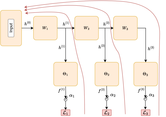
Figure 5: ODL hedge backpropagation. Red lines indicate individual backpropagation calculations.

Now, we consider our proposed architecture, shown in Fig. 6. In our case the weights can be updated using standard backpropagation, i.e., $\mathbf{W}^{(l)}_{t+1}\leftarrow\mathbf{W}^{(l)}_{t}-\eta\nabla_{\mathbf{W}^{(l)}_{t}}\operatorname{\mathcal{L}}$, where $\operatorname{\mathcal{L}}=\sum_{i=1}^{L}\alpha^{(i)}\operatorname{\mathcal{L}}_{i}$.

Lemma 1: The gradient $\frac{\partial\operatorname{\mathcal{L}}_{l}}{\partial\mathbf{W}^{(k)}}=0$ for all $(k,l)\in\{1,2,\dots,L\}^{2}$ with $k>l$.

Proof: Suppose $k>l$ and recall from the definition, $\mathbf{f}^{(l)}=\mathrm{softmax}(\mathbf{h}^{(l)}\Theta^{(l)}),$ with $\mathbf{h}^{(l)}=\sigma(\mathbf{W}^{(l)}\mathbf{h}^{(l-1)}).$ Now following the recursive definition of $\mathbf{h}^{(l)}$ we have:

$$\mathbf{h}^{(l)} =\sigma\left(\mathbf{W}^{(l)}\mathbf{h}^{(l-1)}\right)=\sigma\left(\mathbf{W}^{(l)}\sigma\left(\mathbf{W}^{(l-1)}\sigma\left(\cdots\left(\sigma\left(\mathbf{W}^{(1)}\mathbf{h}^{(0)}\right)\right)\cdots\right)\right)\right)$$ (80)

$$\mathbf{f}^{(l)} =\mathrm{softmax}(\mathbf{h}^{(l)}\Theta^{(l)})=\mathrm{softmax}\left[\sigma\left(\mathbf{W}^{(l)}\sigma\left(\mathbf{W}^{(l-1)}\sigma\left(\cdots\left(\sigma\left(\mathbf{W}^{(1)}\mathbf{h}^{(0)}\right)\right)\cdots\right)\right)\right)\bm{\Theta}^{(l)}\right]$$ (81)

Observe that for $k>l$, $\mathbf{W}^{(k)}$ does not appear in eq. 81 thus we immediately conclude $\frac{\partial\mathbf{f}^{(l)}}{\partial\mathbf{W}^{(k)}}=0$. Recall that the operator $\operatorname{\mathcal{L}}_{l}$ is a function of $\mathbf{f}^{(l)}$, i.e., $\operatorname{\mathcal{L}}_{l}(\mathbf{f}^{(l)},y^{(t)})$. Given that $y^{(t)}$ is a fixed constant, by the chain rule, $\frac{\partial\operatorname{\mathcal{L}}_{l}}{\partial\mathbf{W}^{(k)}}=\frac{\partial\operatorname{\mathcal{L}}_{l}}{\partial\mathbf{f}^{(l)}}\frac{\partial\mathbf{f}^{(l)}}{\partial\mathbf{W}^{(k)}}=0$.

Corollary: 1 $\nabla_{\mathbf{W}^{(k)}_{t}}\operatorname{\mathcal{L}}=\nabla_{\mathbf{W}^{(k)}_{t}}\sum_{i=1}^{L}\alpha^{(i)}\operatorname{\mathcal{L}}_{i}=\nabla_{\mathbf{W}^{(k)}_{t}}\sum_{i=k}^{L}\alpha^{(i)}\operatorname{\mathcal{L}}_{i}$.

Proof: All $i<k$ the terms in the sum are equal to zero by direct application of the previous lemma:

$$\nabla_{\mathbf{W}^{(k)}_{t}}\operatorname{\mathcal{L}} =\nabla_{\mathbf{W}^{(k)}_{t}}\sum_{i=1}^{L}\alpha^{(i)}\operatorname{\mathcal{L}}_{i}=\nabla_{\mathbf{W}^{(k)}_{t}}\sum_{i=1}^{k-1}\alpha^{(i)}\operatorname{\mathcal{L}}_{i}+\nabla_{\mathbf{W}^{(k)}_{t}}\sum_{i=k}^{L}\alpha^{(i)}\operatorname{\mathcal{L}}_{i}$$

$$=\underbrace{\nabla_{\mathbf{W}^{(k)}_{t}}\alpha^{(1)}\operatorname{\mathcal{L}}_{1}}_{=0\text{ by lemma 1}}+\dots+\underbrace{\nabla_{\mathbf{W}^{(k)}_{t}}\alpha^{(k-1)}\operatorname{\mathcal{L}}_{k-1}}_{=0\text{ by lemma 1}}+\nabla_{\mathbf{W}^{(k)}_{t}}\sum_{i=k}^{L}\alpha^{(i)}\operatorname{\mathcal{L}}_{i}$$

$$=\nabla_{\mathbf{W}^{(k)}_{t}}\sum_{i=k}^{L}\alpha^{(i)}\operatorname{\mathcal{L}}_{i}.$$ (82)

Now, using Lemma 1 and by linearity of differentiation we we have:

$$\mathbf{W}^{(3)}_{t+1} =\mathbf{W}^{(3)}_{t}-\eta\nabla_{\mathbf{W}^{(3)}_{t}}\operatorname{\mathcal{L}}=\mathbf{W}^{(3)}_{t}-\eta\nabla_{\mathbf{W}^{(3)}_{t}}\sum_{i=1}^{3}\alpha^{(i)}\operatorname{\mathcal{L}}_{i}=\mathbf{W}^{(3)}_{t}-\eta\nabla_{\mathbf{W}^{(3)}_{t}}\alpha^{(3)}\operatorname{\mathcal{L}}_{3}$$

$$=\mathbf{W}^{(3)}_{t}-\eta\alpha_{3}\frac{\partial\operatorname{\mathcal{L}}_{3}}{\partial\mathbf{f}^{(3)}}\frac{\partial\mathbf{f}^{(3)}}{\partial\mathbf{h}^{(3)}}\frac{\partial\mathbf{h}^{(3)}}{\partial\mathbf{W}^{(3)}_{t}}$$ (83)

$$\mathbf{W}^{(2)}_{t+1} =\mathbf{W}^{(2)}_{t}-\eta\nabla_{\mathbf{W}^{(2)}_{t}}\operatorname{\mathcal{L}}=\mathbf{W}^{(2)}_{t}-\eta\nabla_{\mathbf{W}^{(2)}_{t}}\sum_{i=1}^{3}\alpha^{(i)}\operatorname{\mathcal{L}}_{i}=\mathbf{W}^{(2)}_{t}-\eta\nabla_{\mathbf{W}^{(2)}_{t}}\left(\alpha^{(2)}\operatorname{\mathcal{L}}_{2}+\alpha^{(3)}\operatorname{\mathcal{L}}_{3}\right)$$

$$=\mathbf{W}^{(2)}_{t}-\eta\left(\alpha_{2}\frac{\partial\operatorname{\mathcal{L}}_{2}}{\partial\mathbf{f}^{(2)}}\frac{\partial\mathbf{f}^{(2)}}{\partial\mathbf{h}^{(2)}}\frac{\partial\mathbf{h}^{(2)}}{\partial\mathbf{W}^{(2)}_{t}}+\alpha_{3}\frac{\partial\operatorname{\mathcal{L}}_{3}}{\partial\mathbf{f}^{(3)}}\frac{\partial\mathbf{f}^{(3)}}{\partial\mathbf{h}^{(3)}}\frac{\partial\mathbf{h}^{(3)}}{\partial\mathbf{h}^{(2)}}\frac{\partial\mathbf{h}^{(2)}}{\partial\mathbf{W}^{(2)}_{t}}\right)$$ (84)

$$\mathbf{W}^{(1)}_{t+1} =\mathbf{W}^{(1)}_{t}-\eta\nabla_{\mathbf{W}^{(1)}_{t}}L=\mathbf{W}^{(1)}_{t}-\eta\nabla_{\mathbf{W}^{(1)}_{t}}\sum_{i=1}^{3}\alpha^{(i)}\operatorname{\mathcal{L}}_{i}=\mathbf{W}^{(1)}_{t}-\eta\nabla_{\mathbf{W}^{(1)}_{t}}\left(\alpha^{(1)}\operatorname{\mathcal{L}}_{1}+\alpha^{(2)}\operatorname{\mathcal{L}}_{2}+\alpha^{(3)}\operatorname{\mathcal{L}}_{3}\right)$$

$$=\mathbf{W}^{(1)}_{t}-\eta\Bigg{(}\alpha_{1}\frac{\partial\operatorname{\mathcal{L}}_{1}}{\partial\mathbf{f}^{(1)}}\frac{\partial\mathbf{f}^{(1)}}{\partial\mathbf{h}^{(1)}}\frac{\partial\mathbf{h}^{(1)}}{\partial\mathbf{W}^{(1)}_{t}}+\alpha_{2}\frac{\partial\operatorname{\mathcal{L}}_{2}}{\partial\mathbf{f}^{(2)}}\frac{\partial\mathbf{f}^{(2)}}{\partial\mathbf{h}^{(2)}}\frac{\partial\mathbf{h}^{(2)}}{\partial\mathbf{h}^{(1)}}\frac{\partial\mathbf{h}^{(1)}}{\partial\mathbf{W}^{(1)}_{t}}+\alpha_{3}\frac{\partial\operatorname{\mathcal{L}}_{3}}{\partial\mathbf{f}^{(3)}}\frac{\partial\mathbf{f}^{(3)}}{\partial\mathbf{h}^{(3)}}\frac{\partial\mathbf{h}^{(3)}}{\partial\mathbf{h}^{(2)}}\frac{\partial\mathbf{h}^{(2)}}{\partial\mathbf{h}^{(1)}}\frac{\partial\mathbf{h}^{(1)}}{\partial\mathbf{W}_{t}^{(1)}}\Bigg{)}$$ (85)

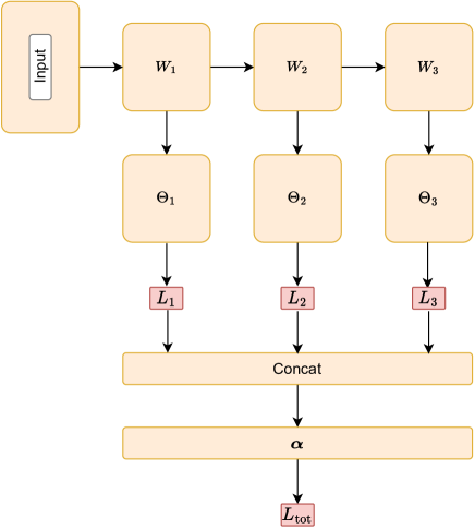
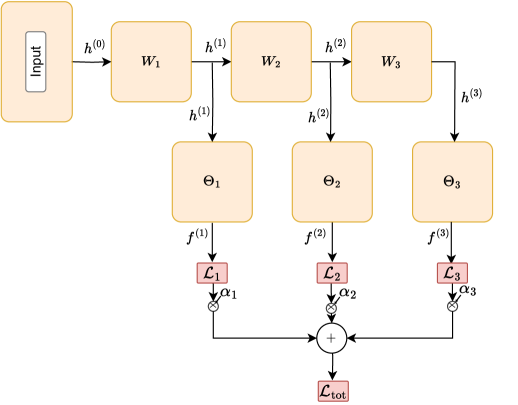
Figure 6: Our proposed architectural modification that provides equivalent total gradients but a more tractable computational graph. There is only one gradient calculation starting from $\operatorname{\mathcal{L}}_{\text{tot}}$. Top and bottom figure show the same architecture, bottom emphasizes that $\alpha_{i}$ is a constant that is not optimized during backprop.

I.2 Complexity analysis

In this section we compare ODL and our proposed modified optimization setup which we call Fast-ODL (FODL) in terms of training time complexity.

ODL training complexity: Consider the computations required to perform an update on hidden layer parameters $\mathbf{W}^{(l)}$. Based on the update rule eq. 76, to update weight matrix $\mathbf{W}^{(l)}$ we need to calculate $L-l+1$ terms in the sum. Assuming that calculating each partial derivative in the previous expressions takes constant time, and noting that the weight update needs to be done for each layer $l\in\{0,1,\dots,L\}$ we obtain a complexity of:

$$\sum_{j=1}^{L}\sum_{i=j}^{L}O(1)=\frac{L(L+1)}{2}=O(L^{2})$$ (86)

per training step. Given that we are in an online learning setting with batch size of 1, in a dataset of size $n$ we are thus going to take $n$ training steps (one step per training datum) for a total training complexity of:

$$\sum_{1}^{n}\sum_{j=1}^{L}\sum_{i=j}^{L}O(1)=O(nL^{2})$$ (87)

The quadratic complexity in the number of layers occurs because of redundant calculations. For example, to update both $\mathbf{W}^{(l)}$ and $\mathbf{W}^{(l-1)}$ we need to compute $\frac{\partial\operatorname{\mathcal{L}}_{l}}{\partial\mathbf{f}^{(l)}}$. However, in the vanilla ODL setup this result is not cached and needs to be recomputed two separate times.

FODL training complexity: Looking at eq. 76, we note that the number of gradient calculations would decrease significantly if the the gradient could be taken outside the sum:

$$W^{(l)}_{t+1}\leftarrow W^{(l)}_{t}-\eta\nabla_{W^{(l)}}\sum_{j=l}^{L}\alpha^{(j)}\operatorname{\mathcal{L}}(\mathbf{f}^{(j)},y_{t}).$$ (88)

However, this expression cannot be directly computed using automatic differentiation as there is no node equal to $\sum_{j=l}^{L}\alpha^{(j)}\operatorname{\mathcal{L}}(\mathbf{f}^{(j)},y_{t})$ is the computational graph in Fig 5. By introducing a concatenation and weighted summation of the intermediate losses, as shown in Fig. 6, we can generate this node and backpropagate from it. Then using PyTorch’s automatic differentiation framework, computed gradients are cached such that there is no redundant calculation, i.e., when updating $\mathbf{W}^{(1)}$ we compute $\frac{\partial\operatorname{\mathcal{L}}_{l}}{\partial\mathbf{f}^{(l)}}$ and store it. Then for all subsequent calculations for updating $\mathbf{W}^{(l)}$ we access the cache at negligible computational cost. This yields a total training cost of:

$$\sum_{1}^{n}\sum_{j=1}^{L}nO(1)=O(nL).$$ (89)

For example, consider computing $\mathbf{W}_{t+1}^{(3)}$ after having computed $\mathbf{W}_{t+1}^{(1)}$. Recalling the equations for their updates shown earlier in this section, we know that:

$$\mathbf{W}^{(3)}_{t+1} =\mathbf{W}^{(3)}_{t}-\eta\alpha_{3}\mathcolor{teal}{\frac{\partial\operatorname{\mathcal{L}}_{3}}{\partial\mathbf{f}^{(3)}}\frac{\partial\mathbf{f}^{(3)}}{\partial\mathbf{h}^{(3)}}}$$

$$\mathbf{W}^{(2)}_{t+1} =\mathbf{W}^{(2)}_{t}-\eta\left(\alpha_{2}\mathcolor{orange}{\frac{\partial\operatorname{\mathcal{L}}_{2}}{\partial\mathbf{f}^{(2)}}\frac{\partial\mathbf{f}^{(2)}}{\partial\mathbf{h}^{(2)}}}\frac{\partial\mathbf{h}^{(2)}}{\partial\mathbf{W}^{(2)}_{t}}+\alpha_{3}\mathcolor{teal}{\frac{\partial\operatorname{\mathcal{L}}_{3}}{\partial\mathbf{f}^{(3)}}\frac{\partial\mathbf{f}^{(3)}}{\partial\mathbf{h}^{(3)}}}\mathcolor{orange}{\frac{\partial\mathbf{h}^{(3)}}{\partial\mathbf{h}^{(2)}}}\frac{\partial\mathbf{h}^{(2)}}{\partial\mathbf{W}^{(2)}_{t}}\right)$$

$$\mathbf{W}^{(1)}_{t+1} =\mathbf{W}^{(1)}_{t}-\eta\Bigg{(}\alpha_{1}\frac{\partial\operatorname{\mathcal{L}}_{1}}{\partial\mathbf{f}^{(1)}}\frac{\partial\mathbf{f}^{(1)}}{\partial\mathbf{h}^{(1)}}\frac{\partial\mathbf{h}^{(1)}}{\partial\mathbf{W}^{(1)}_{t}}+\alpha_{2}\mathcolor{orange}{\frac{\partial\operatorname{\mathcal{L}}_{2}}{\partial\mathbf{f}^{(2)}}\frac{\partial\mathbf{f}^{(2)}}{\partial\mathbf{h}^{(2)}}}\frac{\partial\mathbf{h}^{(2)}}{\partial\mathbf{h}^{(1)}}\frac{\partial\mathbf{h}^{(1)}}{\partial\mathbf{W}^{(1)}_{t}}$$

$$\quad\quad\quad\quad\quad\quad+\alpha_{3}\mathcolor{teal}{\frac{\partial\operatorname{\mathcal{L}}_{3}}{\partial\mathbf{f}^{(3)}}\frac{\partial\mathbf{f}^{(3)}}{\partial\mathbf{h}^{(3)}}}\mathcolor{orange}{\frac{\partial\mathbf{h}^{(3)}}{\partial\mathbf{h}^{(2)}}}\frac{\partial\mathbf{h}^{(2)}}{\partial\mathbf{h}^{(1)}}\frac{\partial\mathbf{h}^{(1)}}{\partial\mathbf{W}^{(1)}_{t}}\Bigg{)}$$

Clearly, caching the term in teal would reduce computation. Thus, in FODL computing the update for the first layer $\mathbf{W}^{(1)}_{t+1}$ and storing all the partial derivatives along the computational graph provides all the necessary information to calculate $\mathbf{W}^{(2)}_{t+1},\dots,\mathbf{W}^{(L)}_{t+1}$ with computing only one new derivative $\frac{\partial\mathbf{h}^{(l)}}{\partial\mathbf{W}^{(l)}_{t}}$. Similarly this holds for computing $\mathbf{W}^{(2)}_{t+1}$ after $\mathbf{W}^{(1)}_{t+1}$, see orange terms.

More precisely, in the standard ODL formulation the redundancy of the teal term is very high as it is computed $L$ times (the terms in orange $L-1$ times) but in our formulation every gradient is only computed once. This yields a total computational saving of:

$$\sum_{1}^{n}\sum_{j=1}^{L}\sum_{i=j+1}^{L}=n\frac{L(L-1)}{2}O(1).$$ (90)

By subtracting the amount of computation saved by FastODL from the total complexity of the base ODL method we obtain the complexity of our proposed approach and it is linear:

$$\sum_{1}^{n}\sum_{j=1}^{L}\sum_{i=j}^{L}O(1)-\sum_{1}^{n}\sum_{j=1}^{L}\sum_{i=j+1}^{L}O(1)=n\left(\frac{L(L+1)}{2}-\frac{L(L-1)}{2}\right)O(1)=nLO(1)=O(nL).$$ (91)

References

- Abdel Wahab [2022] Omar Abdel Wahab. Intrusion detection in the IoT under data and concept drifts: Online deep learning approach. IEEE J. Internet of Things, 9(20):19706–19716, 2022.
- Agarwal et al. [2021] Naman Agarwal, Satyen Kale, and Julian Zimmert. Efficient methods for online multiclass logistic regression. In Proc. Int. Conf. Alg. Learning Theory (ALT), Online, Mar. 2021.
- Agarwal et al. [2023] Rohit Agarwal, Deepak Gupta, Alexander Horsch, and Dilip K. Prasad. Aux-drop: Handling haphazard inputs in online learning using auxiliary dropouts. Trans. Mach. Learn. Research (TMLR), 2023. ISSN 2835-8856.
- Baldi et al. [2014] Pierre Baldi, Peter Sadowski, and Daniel Whiteson. Searching for exotic particles in high-energy physics with deep learning. Nature Communications, 5, 2014.
- Bartlett et al. [2007] Peter L. Bartlett, Elad Hazan, and Alexander Rakhlin. Adaptive online gradient descent. In Proc. Neural Info. Proces. Sys. (NIPS), page 65–72, Red Hook, NY, USA, Dec. 2007.
- Basaglia et al. [2023] T. Basaglia, Matthew Bellis, Jakob Blomer, J. Boyd, C. Bozzi, Daniel Britzger, S. Campana, Concetta Cartaro, G. M. Chen, B. Couturier, G. David, C. Diaconu, A. Dobrin, Dirk Duellmann, M. Ebert, Peter Elmer, J. Fernandes, L. Fields, P. Fokianos, Gerardo Ganis, Achim Geiser, Mihaela Gheata, J. B. Gonzalez Lopez, T. Hara, L. Heinrich, Michael D. Hildreth, Ken Herner, Bo Jayatilaka, M. Kado, Oliver Keeble, Alexander Kohls, K. Naim, Clemens Lange, Kati Lassila-Perini, Sergey Levonian, Mario Maggi, Zach Marshall, Pere Mato Vila, A. Mecionis, A. Morris, S. Piano, Maxim Potekhin, M. Schröder, Ulrich Schwickerath, Elizabeth Sexton-Kennedy, Thomas Simko, T. Smith, D. South, A. Verbytskyi, Michel Vidal, A. Vivace, L Wang, Gill Watt, Torre J. Wenaus, and DPHEP Collaboration. Data preservation in high energy physics. Euro. Phys. J. C, 83:1–41, 2023.
- Belkin et al. [2006] Mikhail Belkin, Partha Niyogi, and Vikas Sindhwani. Manifold regularization: A geometric framework for learning from labeled and unlabeled examples. J. Mach. Learn. Res., 7:2399–2434, 2006.
- Beyazit et al. [2019] Ege Beyazit, Jeevithan Alagurajah, and Xindong Wu. Online learning from data streams with varying feature spaces. In Proc. Conf. Artificial Intell. (AAAI), pages 3232–3239, Feb. 2019. ISBN 978-1-57735-809-1.
- Böhning [1992] Dankmar Böhning. Multinomial logistic regression algorithm. Annals of the Institute of Statistical Mathematics, 44:197–200, 1992.
- Bottou [1998] Léon Bottou. Online Learning and Stochastic Approximations, chapter 2, pages 9–42. Cambridge University Press, 1998.
- Bottou and LeCun [2003] Léon Bottou and Yann LeCun. Large scale online learning. In Proc. Adv. Neural Info. Proces. Sys. (NIPS), pages 217–224, Vancouver, Canada, Dec. 2003.
- Chang and Lin [2011] Chih-Chung Chang and Chih-Jen Lin. Libsvm: A library for support vector machines. ACM Trans. Intell. Syst. Technol., 2(3), may 2011. ISSN 2157-6904.
- de Vilmarest and Wintenberger [2021] Joseph de Vilmarest and Olivier Wintenberger. Stochastic online optimization using kalman recursion. J. Machine Learning Research, 22(223):1–55, 2021.
- Dredze et al. [2008] Mark Dredze, Koby Crammer, and Fernando Pereira. Confidence-weighted linear classification. In Proc. Int. Conf. Machine Learning (ICML), page 264–271, Helsinki, Finland, Jul. 2008.
- Dua et al. [2017] Dheeru Dua, Casey Graff, et al. Uci machine learning repository, 2017.
- Freund and Schapire [1997] Yoav Freund and Robert E Schapire. A decision-theoretic generalization of on-line learning and an application to boosting. Journal of Computer and System Sciences, 55(1):119–139, 1997. ISSN 0022-0000.
- Graas et al. [2023] Adriaan B.M. Graas, Sophia Bethany Coban, Kees Joost Batenburg, and Felix Lucka. Just-in-time deep learning for real-time x-ray computed tomography. Scientific Reports, 13, 2023.
- Guha et al. [2000] Sudipto Guha, Nina Mishra, Rajeev Motwani, and Liadan O’Callaghan. Clustering data streams. In Proc. Foundations Comp. Science, (FOCS), pages 359–366, Redondo Beach, California, USA, Nov. 2000.
- Hazan et al. [2007] Elad Hazan, Amit Agarwal, and Satyen Kale. Logarithmic regret algorithms for online convex optimization. Mach. Learn., 69(2-3):169–192, 2007.
- He et al. [2019] Yi He, Baijun Wu, Di Wu, Ege Beyazit, Sheng Chen, and Xindong Wu. Online learning from capricious data streams: A generative approach. In Proc. Int. Joint Conf. on Artificial Intell. (IJCAI), pages 2491–2497, Jul. 2019.
- Hoi et al. [2013] Steven C. H. Hoi, Rong Jin, Peilin Zhao, and Tianbao Yang. Online multiple kernel classification. Mach. Learn., 90(2):289–316, 2013.
- Hu et al. [2021] Xinyue Hu, Haoji Hu, Saurabh Verma, and Zhi-Li Zhang. Physics-guided deep neural networks for power flow analysis. IEEE Trans. Power Systems, 36(3):2082–2092, 2021.
- Li et al. [2020] Shunkai Li, Xin Wang, Yingdian Cao, Fei Xue, Zike Yan, and Hongbin Zha. Self-supervised deep visual odometry with online adaptation. In Proc. IEEE/CVF Conf. Comp. Vision Pattern Recognition (CVPR), pages 6339–6348, Online, Jun. 2020.
- Liu et al. [2022] ZK Liu, LH Zhang, B Liu, ZY Zhang, GC Guo, DS Ding, and BS Shi. Deep learning enhanced Rydberg multifrequency microwave recognition. Nature Commun., 13(1997):1–10, 2022.
- Min et al. [2022] Youngjae Min, Kwangjun Ahn, and Navid Azizan. One-pass learning via bridging orthogonal gradient descent and recursive least-squares. In Proc. IEEE Conf. Decision & Control (CDC), pages 4720–4725, 2022.
- Oreshkin et al. [2022] Boris N. Oreshkin, Florent Bocquelet, Félix G. Harvey, Bay Raitt, and Dominic Laflamme. Protores: Proto-residual network for pose authoring via learned inverse kinematics. In Proc. Int. Conf. Learning Representations (ICLR), Online, Apr. 2022.
- Sahoo et al. [2018] Doyen Sahoo, Quang Pham, Jing Lu, and Steven C. H. Hoi. Online deep learning: learning deep neural networks on the fly. In Proc. Int. Joint Conf. Artificial Intelligence (IJCAI), page 2660–2666, Stockholm, Sweden, Jul. 2018.
- Shao et al. [2021] Zhou Shao, Sha Yuan, and Yongli Wang. Adaptive online learning for iot botnet detection. Information Sciences, 574:84–95, 2021. ISSN 0020-0255.
- Yang et al. [2022] Luyu Yang, Mingfei Gao, Zeyuan Chen, Ran Xu, Abhinav Shrivastava, and Chetan Ramaiah. Burn after reading: Online adaptation for cross-domain streaming data. In Proc. Euro. Conf. Comp. Vision (ECCV), page 404–422, Tel Aviv, Israel, Oct. 2022.
- Zhang et al. [2020] Huanhuan Zhang, Anfu Zhou, Jiamin Lu, Ruoxuan Ma, Yuhan Hu, Cong Li, Xinyu Zhang, Huadong Ma, and Xiaojiang Chen. Onrl: improving mobile video telephony via online reinforcement learning. In Proc. Int. Conf. Mobile Comp. Networking, pages 1–14, London, United Kingdom, Sep. 2020.
- Zinkevich [2003] Martin A. Zinkevich. Online convex programming and generalized infinitesimal gradient ascent. In Proc. Int. Conf. Machine Learning (ICML), Washington, DC, USA, Aug. 2003.