Department of Engineering Cybernetics
TTK4551 - Specialization Project

 

Identifiability, Observability, Uncertainty and Bayesian System Identification of Epidemiological Models
 

Jonas Hjulstad

May, 2021

1 Introduction

1.1 Background

Variants of deterministic, compartmental models have been developed to model epidemics for over a century, starting with bilinear dynamics proposed in 1906 [[9]], further developed to a three-compartment model called the Kermack-Mckendrick model (SIR) in 1927 [[14]]. The dynamics of these models are well understood and favorable for analytical purposes, but the models are limited to capturing the dynamics of large, homogenous populations.

Past epidemics in the 20th century have re-ignited the interest for epidemic modeling in general, including the use of network models and stochastic designs, in order to capture the dynamics of heterogenous populations. In the shortcomings for deterministic models in small populations or initial/endemic stages of a disease, stochastic models manage to capture the events, but the number of possible outcomes for these models may be large. Network models have also been used for a long time in epidemiology, originating from the study of graphs by Erdös and Rényi [[23]]. These models makes it possible to specify the structure within the population, but falls short on the analytical properties, making it harder to determine and relate the reproduction number $\mathscr{R}_{0}$ and final size of the epidemic.

The advantages of network models have been adressed by NTNUs COVID-19 modelling taskforce [[6]], a model that introduce a metapopulation model fitted to capture social contact in schools, workplaces, nursing homes and hospitals in Trondheim and Oslo.

Stochastic differential equations were introduced earlier by Reed and Frost in 1928 [[1]], which introduced random binomially distributed infections to compartmental models. These fall under the category of Chain-Binomial models, which model the chance of escaping infection and other transitions as a series of Bernoulli trials. These models have better analytical properties than network models, but they do not use spatial information, which makes the overall uncertainty of the model much larger.

1.2 Problem Statement

The objective of this project is to study structural identifiability and state observability of simple, compartmental epidemiological models, specifically SIR/SEIR/SEIAR models. In addition, the representation of uncertainty in simple compartmental models should be addressed, and how the uncertainty in simple compartmental models can be represented by appropriately selecting parameter distributions in the corresponding stochastic version of the same compartmental models. The focus should be on moderately sized populations where the assumptions underlying a deterministic approximation do not hold.

The project should:

• Provide an introduction to the probability distributions used to describe uncertainty in epidemiological models

• Provide an introduction to SIR/SEIR/SEIAR-type compartmental epidemiological models.

• Analyze structural identifiability and observability in the deterministic compartmental models.

• Study how stochastic Chain-Binomial models can be used to generate parameter distributions for compartmental models. To this end, Sequential Monte Carlo- and Markov Chain Monte Carlo-based methods should be studied.

• Create a software library with an efficient SMC/MCMC-sampler capable of estimating parameter distriutions for the introduced models.

1.3 Motivation

There are several reasons for investigating the aforementioned topics. Relating deterministic to stochastic models is an important step towards connecting the models to true epidemics, which are very stochastic by nature. This is also a first step towards relating the deterministic model to network models, for which there exist ways of assessing model parameters on a smaller scale, which as a consequence results in overparametrized, complex models. Finding reasonable approximations can reduce the computational expense of simulations, and make it possible to retrieve locally valid, analytical solutions which makes it easier to understand the course of the epidemic itself.

Another reason is controlling the outcome of epidemics. Numerical optimal control is a well established field for deterministic models, which makes the deterministic approximations very attractive as long as they remain valid. Considering that political decisions in an epidemic may have lethal consequences, it is important that robust control strategies are implemented, which in turn requires the validity of model approximations to be well understood.

1.4 Software

Python was initially chosen as programming language for this project, but computational efficiency moved parts of the project over to C++. Compatibility issues and challenges with the building of C++ libraries and Python dependencies made Ubuntu a more attractive operating system.

Software	Version	Description	Software	Version	Description
Python	3.8	Interpreter	Matplotlib	3.4.1	Plotting
PyMC3	3.11.2	SMC/MCMC	Theano-PyMC	1.1.2	Optimized Compilation
Scipy	1.6.3	Sampling and Integration
C++	ISO C++14	Language Standard	g++	9.3.0	Compiler
CMake	3.16.3	Build automation	GSL	2.5	Standard Library
Ubuntu	20.04.02 LTS	Operating System

Table 1: Software and libraries used

2 Probability Distributions and Dispersion

Epidemics are in general well approximated by deterministic differential equations when the susceptible and infected groups of a large population are homogenously distributed and of equal size. This does not hold at the time of outbreak and close to the endemic timepoint, where the number of infected is smaller. The deterministic models also fail to capture the dynamics of smaller populations.

As an alternative to deterministic dynamics, it is possible to model infections, exposure and recovery with probabilities. The distributions necessary to model these effects are introduced in this section. In some cases of modeling, the variance of a distribution may be expected to be higher than the base variance of the candidate distribution. In this case the model is overdispersed, which will be shown to be implementable by combining distributions.

2.1 Binomial Distribution

The Binomial distribution captures the probability of $k$ successful Bernoulli trials (with probability $p$) occuring in $n$ attempts. Its probability mass function (PMF) is given by:

$$P_{PMF}(X=k|n,p)=\binom{n}{k}p^{k}(1-p)^{n-k}\triangleq\text{Bin}(k,n,p)$$ (1)

The distribution has an expected value of $np$ with variance $np(1-p)$. The Binomial distribution is useful for modeling infections and recoveries when they are considered to be independent trials with equal probability. The variance of the distribution converges to the mean when the number of trials is large, and the probability is small ($np(1-p)\approx np$ when $n>>p$).

2.2 The Poisson Distribution

The Poisson distribution captures the probability of a number of events k to occur in a time interval $t$ with event rate $r$. Its PMF is parametrized by the expected number of events $\lambda=rt$.

$$P_{PMF}(X=k|\lambda)=\frac{\lambda^{k}e^{-\lambda}}{k!}\triangleq\text{Po}(k,\lambda)$$ (2)

The distribution models systems with a large number of possible, rare events well, but fails to represent where probabilities are higher or the number of events lower.

2.3 Gamma Distribution

The Gamma distribution is parametrized with $\alpha$ and $\gamma$, giving the following Probability Density Function (PDF):

$$P_{PDF}(X=k|\alpha,\beta)=\frac{\beta^{\alpha}k^{\alpha-1}e^{-\beta k}}{\Gamma(\alpha)}\triangleq\text{Gamma}(k,\alpha,\beta)$$ (3)

Where $\Gamma(\alpha)$ is the gammma function. The distribution has important relations to the exponential and normal distributions, and is a popular choice to combine with other distributions to get desired properties of moments.

2.4 Negative Binomial Distribution

The Negative Binomial distribution can be seen as a gamma-distributed variable drawn from a Poisson distribution, where the PMF is given by:

$$P_{PMF}(X=k|\lambda,r)=\frac{\lambda^{k}}{k!}\frac{\Gamma(\lambda+k)}{\Gamma(r)(r+\lambda)^{k}}\frac{1}{(1+r)^{r}}\triangleq\text{NegBin}(k,\lambda,r)$$ (4)

The Poisson-Gamma relationship to the Binomial distribution is seen by marginalizing the joint distribution of $\lambda,k$ with respect to $\lambda$:

$$\text{NegBin}(X=k|\lambda,r)=\int_{0}^{\infty}\text{Poisson}(k,\lambda)\text{Gamma}(X=\lambda,\alpha=r,\beta=\frac{1-p}{p})d\lambda$$ (5)

Where $r$ is the number of failures to be drawn from a set of $k$ bernoulli trials with success-probability $p$ and mean $\lambda=\frac{pr}{1-p}$. When the number of failures to draw approaches infinity, the Negative Binomial distribution converges towards the Poisson distribution:

$$\lim_{r\rightarrow\infty}=\frac{\lambda^{k}}{k!}\frac{1}{1}\frac{1}{e^{\lambda}}$$ (6)

For finite values of $r$ the mean and variance of the distribution is shifted to represent overdispersion. This can also be seen in the variance of the distribution:

$$\lim_{r\rightarrow\infty}E[(x-\bar{x})^{T}(x-\bar{x})]=\lim_{r\rightarrow\infty}\lambda(1+\frac{\lambda}{r})=\lambda$$ (7)

Setting $\nu=\frac{\lambda}{r}$ makes it possible to scale the distribution variance with $\nu$ proportionally to the Poisson base variance $\lambda$.

2.5 Beta Distribution

Similar to the Gamma distribution the Beta distribution is another choice to adjust moments of distributions. It can be considered a function of two Gamma-distributed variables:

$$\begin{split}\frac{X}{X+Y}&\sim\text{Beta}(\alpha,\beta)\\ X\sim\text{Gamma}(\alpha,1)&,\quad Y\sim\text{Gamma}(\beta,1)\end{split}$$ (8)

This results in the following PDF:

$$P_{PDF}(X=k|\alpha,\beta)=\frac{1}{B(\alpha,\beta)}k^{\alpha-1}(1-k)^{\beta-1}\triangleq\text{Beta}(\alpha,\beta)$$ (9)

Where $B(\alpha,\beta)$ is the Beta function.

2.6 Beta-Binomial Distribution

The Beta-Binomial distribution can be seen as a Binomial distribution where $p$ is drawn randomly from a Beta-distribution with the following PMF:

$$P_{PMF}(X=k|\alpha,\beta,n)=\binom{n}{k}\frac{B(k+\alpha,n-k+\beta)}{B(\alpha,\beta)}\triangleq\text{BetaBin}(\alpha,\beta,n)$$ (10)

The first moments are given by equations 11, 12.

$$E[X] =\frac{n\alpha}{\alpha+\beta}$$ (11)

$$E[(X-\bar{x})^{T}(X-\bar{x})] =\frac{n\alpha\beta(\alpha+\beta+n)}{(\alpha+\beta)^{2}(\alpha+\beta+1)}$$ (12)

This distribution will only be used for overdispersion of the Binomial distribution, but it should be noted that a relation to the Poisson distribution can be derived through marginalization much in the same way as the Negative Binomial distribution.

The relationship between the Beta, Binomial and Beta-Binomial distributions is seen by marginalizing the joint distribution of $p,k$ with respect to $p$.

$$\text{BetaBin}(X=k|p,n)=\int_{0}^{1}\text{Bin}(k|n,p)\text{Beta}(p|\alpha,\beta)dp$$ (13)

By assigning $\mu=\frac{\alpha}{\alpha+\beta}$ and $\gamma=\frac{1}{\alpha+\beta+1}$ the first moments can be reparametrized.

$$E[X] =n\mu$$ (14)

$$E[(X-\bar{x})^{T}(X-\bar{x})] =n\mu(1-\mu)(1+(n-1)\gamma)$$ (15)

$\gamma\in(0,1)$ is the dispersion parameter. When $\gamma\rightarrow 0$ the distribution variance converges to the variance of the Binomial distribution. Setting $\gamma=\frac{\nu}{n-1}$ makes it possible to scale the distribution variance with $\nu$ proportionally to the Binomial base variance $n\mu(1-\mu)$.

2.7 Comparison of Distributions and Limitations

Given a small probability $p$ and large sample size $n$, the Poisson distribution approximates the Binomial distribution well, even with overdispersion. Figure 1 illustrates differences in dispersion for the approximations.

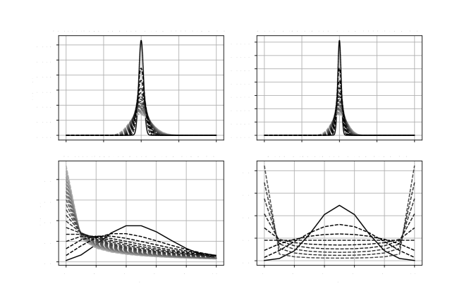
Figure 1: Comparison of overdispersion using PMFs for the Poisson, Negative Binomial, Binomial and Beta Binomial distributions. The dispersion is linearly spaced with additional $\nu=[1,\dots,8]$ standard deviations compared to the base distributions.

The Poisson distribution keeps the same shape as the Binomial distribution even when the approximation is bad, but the Negative Binomial and Beta Binomial distributions become very different in this case. It is therefore very important to ensure that Poisson approximations remain valid for the whole trajectory if they are to be used.

3 Epidemiological Models

The stochastic models introduced are based on terms from a demographic, stochastic SEIR-model [[10]]. The demographic terms excluded in order to retain the property of a constant total population. Poisson and Binomial distributions are used to present the dynamics, which respectively can be replaced with negative Binomial and Beta-Binomial distributions to model overdispersion (Section 2).

Deterministic and corresponding Chain-Binomial models are introduced for the classic SIR, SEIR and SEIAR compartmental models, followed by trajectory simulations to compare the deterministic and stochastic models for small populations. The initial state is set to a timepoint after the initial outbreak, which is captured by the following deterministic parameters:

$\Delta t$	$1[\text{Day}]$	$T_{\text{span}}$	$[0,201][\text{Days}]$	$S_{0}$	$9000/900\text{(SIR)}$
$\mathscr{R}_{0}$	$1.2$	$\alpha$	$0.11$	$I_{0}$	$1000/100\text{(SIR)}$
$\beta$	$0.13$	$\gamma$	$0.33$	$R_{0}$	$0$
$\mu$	0.11	p	0.5	$N_{pop}$	$10000/1000\text{(SIR)}$

Table 2: Deterministic parameters used for epidemiological models

3.1 SIR Model

The SIR discrete model is minimal in its number of compartments for modeling epidemics without periodicity. The average contact rate per person $\beta$ and recovery rate $\alpha$ are the only parameters required to describe an asymptotically stable epidemic.

Deterministic:

$$\begin{split}\dot{S}&=S-\beta\frac{SI}{N_{pop}}\\ \dot{I}&=I+\beta\frac{SI}{N_{pop}}-\alpha I\\ \dot{R}&=R+\alpha I\end{split}$$ (16)

The Susceptible ($N$), Infected ($I$) and Recovered ($R$) population groups adds up to total population $N$ at all timesteps. Given an constant population $N_{pop}$ the third equation can be omitted and retrieved post-simulation as $R(t)=N_{pop}-S(t)-I(t)$.

Stochastic:

$$\begin{split}\Delta S&=-\text{Po}(S_{k}\cdot p_{I}(t))\\ \Delta I&=\text{Po}(S_{k}\cdot p_{I}(t))-\text{Bin}(I_{k},p_{R})\\ \Delta R&=\text{Bin}(I_{k},p_{R})\end{split}$$ (17)

Where $p_{I}(t)=1-\text{exp}[-\beta c(t)\frac{I(t)}{N_{pop}}\Delta t]$, and $\beta,c(t)$ are the transmission probability and contact rate respectively. Fixed probabilities can be fitted to the deterministic model, yielding $p_{R}=1-\text{exp}(-\alpha\Delta t)$.

Note: With some abuse of notation, the probability-distributed variables are drawn once every iteration (e.g. $\text{Po}(S_{k}\cdot p_{I}(t))$ is the same sample for $\Delta S,\Delta I$ in equation 17, not two samples from the same distribution).

3.1.1 Simulated Trajectories

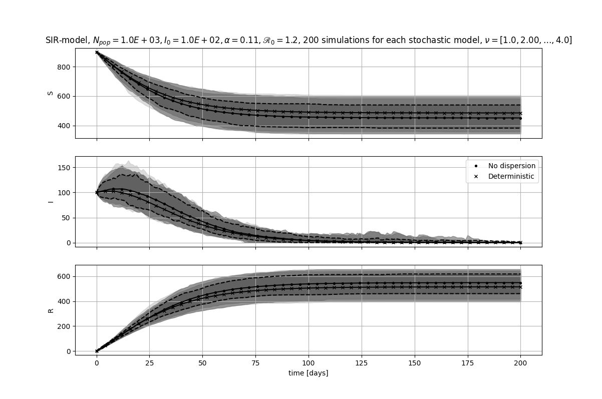
Figure 2: Comparison of dispersed trajectories for SIR-model ($90$-percentiles from both sides of the stochastic simulation mean). Increasing $\nu$ gradually fades in to gray. 90-percentiles for undispersed trajectory is shown in dotted lines.

3.2 SEIR Model

An intermediate stage can be added to the SIR model in order to model incubation period. This compartment is very relevant for the current pandemic, considering the expected average incubation period of $5.1$ days[[16]] for COVID-19.

Deterministic:

$$\begin{split}\dot{S}&=-\beta\frac{SI}{N_{pop}}\\ \dot{E}&=\beta\frac{SI}{N_{pop}}-\gamma E\\ \dot{I}&=\gamma E-\alpha I\\ \dot{R}&=\alpha I\end{split}$$ (18)

Stochastic:

$$\begin{split}\Delta S&=-\text{Po}(S_{k}\cdot p_{E}(t))\\ \Delta E&=\text{Po}(S_{k}\cdot p_{E}(t))-\text{Bin}(E_{k},p_{I})\\ \Delta I&=\text{Bin}(E_{k},p_{I})-\text{Bin}(I_{k},p_{R})\\ \Delta R&=\text{Bin}(I_{k},p_{R})\end{split}$$ (19)

Where $p_{E}(t)=1-\text{exp}[-\beta c(t)\frac{I(t)}{N_{pop}}\Delta t]$ and $p_{I}=1-\text{exp}(-\gamma\Delta t)$.

3.2.1 Simulated Trajectories

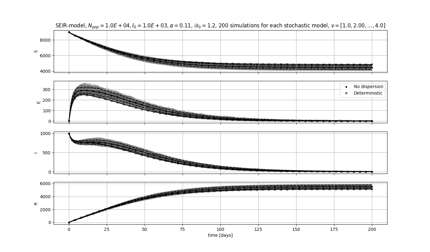
Figure 3: Comparison of dispersed trajectories for SEIR-model ($90$-percentiles from both sides of the stochastic simulation mean). Increasing $\nu$ gradually fades in to gray. 90-percentiles for undispersed trajectory is shown in dotted lines.

3.3 SEIAR Model

Testing unavailability and high estimated asymptomatic rates for COVID-19[[27]], indicates that there should be an alternative compartment for some infected individuals. A SIR/SEIR model fitted on observed infections will not be able to account for undetected infections, which is why an asymptomatic group is introduced.

Deterministic:

$$\begin{split}\dot{S}&=-\beta\frac{S(I+A)}{N_{pop}}\\ \dot{E}&=\frac{S(I+A)}{N_{pop}}-\gamma E\\ \dot{I}&=\gamma pE-\alpha I\\ \dot{A}&=\gamma(1-p)E-\mu A\\ \dot{R}&=\alpha I+\mu A\end{split}$$ (20)

The fraction of exposed turning infectious is described by $p$, and the recovery rate of the asymptomatic group is described by $\mu$.

Stochastic:

$$\begin{split}\Delta S&=-\text{Po}(S_{k}\cdot p_{E}(t))\\ \Delta E&=\text{Po}(S_{k}\cdot p_{E}(t))-\text{Bin}(E_{k},p_{I})-\text{Bin}(E_{k},p_{A})\\ \Delta I&=\text{Bin}(E_{k},p_{I})-\text{Bin}(I_{k},p_{R,I})\\ \Delta A&=\text{Bin}(E_{k},p_{A})-\text{Bin}(A_{k},p_{R,A})\\ \Delta R&=\text{Bin}(I_{k},p_{R,I})+\text{Bin}(A_{k},p_{R,A})\end{split}$$ (21)

Where $p_{E}(t)=1-\text{exp}[-\beta c(t)\frac{I(t)+A(t)}{N_{pop}}\Delta t]$, $p_{I}=1-\text{exp}(-p\gamma\Delta t)$ and $p_{A}=1-\text{exp}(-(1-p)\gamma\Delta t)$. $p_{A,R},p_{I,R}$ follows the same pattern.

3.3.1 Simulated Trajectories

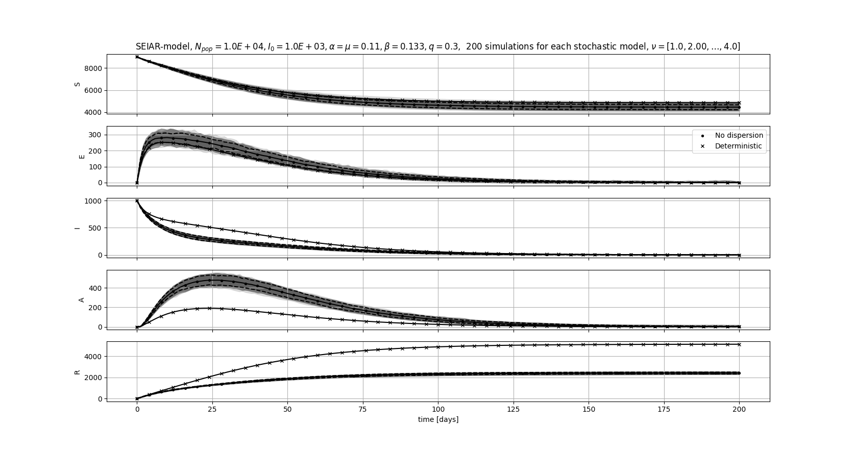
Figure 4: Comparison of dispersed trajectories for SEIAR-model ($90$-percentiles from both sides of the stochastic simulation mean). Increasing $\nu$ gradually fades in to gray. 90-percentiles for undispersed trajectory is shown in dotted lines.

3.4 A Simulation of the Initial Outbreak

With a smaller number of initial infected, the interval of outcomes becomes much larger.

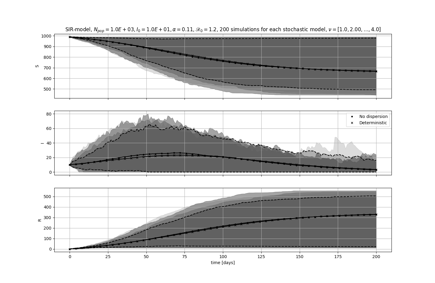
Figure 5: Comparison of dispersed trajectories for SIR-model ($90$-percentiles from both sides of the stochastic simulation mean). Increasing $\nu$ gradually fades in to gray. 90-percentiles for undispersed trajectory is shown in dotted lines.

3.5 Remarks on the Simulations

The parameters used was specifically chosen to yield trajectories sensitive to distribution variance, where the average mean trajectory still is relatable to the deterministic one.

Stochastic SEIR/SEIAR has one extra binomial term in the connection between the susceptible and the infected group, which results in an overall variance increase in the resulting trajectories. In order to illustrate trajectories on a comparable scale, the total population in SEIR/SEIAR-simuations is larger.

For the total population size $N_{pop}=10000/1000(SIR)$ with $\Delta t=1[\text{Day}]$ the mean stochastic trajectory is not approximately equal to the deterministic. This changes when the exponent in the binomial probabilities ($p_{I},p_{E},p_{A}$, ..) converges towards $0$, which is achieved by increasing $N_{pop}$ or decreasing $\Delta t$.

The asymmetric 90-percentiles in the illustrations are not approximately equal to the true confidence intervals. The methods implemented to obtain true confidence intervals in Python ended up becoming too computationally expensive to evaluate. If more accurate intervals are needed in the future, a reimplementation in C++ could be considered.

The dispersion parameter $\nu$ was expected to have a larger impact. Increasing the variance by a factor of 5 ($\nu=4$) was expected to drastically impact the resulting trajectories, but they remain comparatively close for this population size. Further reducing the population size enhances the effect of the dispersion, but also separates the stochastic mean from the deterministic trajectory. The 90-percentiles may be decieving in this case, a better approximation of the true confidence intervals may be needed.

3.6 Discussion

The small effect of overdispersion on the trajectories for populations with homogenous initial populations is promising for the deterministic approximation. If the deterministic approximation remains valid for parts of the epidemic, it becomes possible to consider applying numerical optimal control directly on the model equations, which is a much simpler approach than the robust alternatives needed for stochastic models.

However, when trajectories are simulated from the initial stage of an outbreak (figure 5) the 90-percentiles cover a much larger region of the state space. Performing optimal control on a deterministic approximation could in this case result in solutions which underestimates the infectious spread, and should therefore be avoided. The space of possible outcomes is very large for Chain Binomials under these conditions, which raises the need for individual based modeling.

The different regions of validity shows that an understanding of a true epidemic may require the use of multiple models, where each model is valid in different regions. It is reasonable to assume that the initial outbreak is better modeled with spatial information and a more detailed description of each individuals dynamic.

The 90 percentiles produced with no dispersion covers a significant region. The effect of underdispersion should be investigated to address this.

4 Identifiability

Verifying the performance of estimators is challenging with low availability of data. A previous approach to optimal control of the COVID-19 pandemic ([[21]]) have addressed this by bounding the parameter space to reasonable limits before performing the identification. Even with a restricted parameter space, it is still uncertain if the data is informative enough to distinguish the parameter values, or if the resulting model will be overfitted. With reasonable parameter ranges, this can still be solved with robust control strategies ([[15]]), but this does not solve the validation-issues of the models.

One solution ([[19]] have split data into training/validation datasets to verify the performance of identified parameters. While verifying the model on currently available data makes is a good practice for confirming how well it performs in a local region, it goes not guarantee good prediction performance for the future.

Before performing parameter identification, it is important to determine if some parameters even are identifiable at all. This is done by evaluating the structural idenitifiability, which in the following sections will be done algebraically by hand and with specifically designed software.

4.1 Differential Algebra for Identifiability of Systems

Differential Algebra for Identifiability of SYstems (DAISY) [[4]] is a software tool used to assess global/local identifiability of parameters in polynomial/rational models. It is based on the general-purpose algebra system REDUCE [[11]], and can be used to determine the parameter identifiability in some of the presented epidemiological models.

4.1.1 Ranking

DAISY uses an algorithm which requires a variable ranking of the inputs, outputs and internal states of the subject system and their derivatives. The ranking does not impact the outcome of the algorithm, but may reduce the number of divisions needed to produce results.

$$u_{1}<u_{2} <\dots<y_{1}<y_{2}<\dots\dot{u}_{1}<\dot{u}_{2}<\dots<\ddot{u}_{1}<\ddot{u}_{2}$$ (22)

$$<\dots< \dot{y}_{1}<\dot{y}_{2}<\dots<\ddot{y}_{1}<\ddot{y}_{2}<\dot{x}_{1}<\dot{x}_{2}<\dots$$

For a polynomial $A_{i}$ the term containing the highest ranked variable (or highest ranked variable product, e.g. $\dot{x}_{1}y_{1}<\dot{x}_{1}\dot{y}_{1}$) is called the leader term.

4.1.2 Pseudodivision Algorithm

To determine the uniqueness of parameter solutions it is desired to find the characteristic set of the subject system. The characteristic set is a minimal set of differential polynomials which generates the same differential ideal as an arbitrary set of the same polynomials. A polynomial $A_{i}$ is said to be reduced wrt. $A_{j}$ if it does not contain any algebraic degreee of $A_{j}$’s leader term or its derivatives. With the previous definitions, Ritt’s pseudodivision algorithm [[24]] can be summarized in three steps:

1. If polynomial $A_{i}$ contains the $k$th derivative of $A_{j}$’s leader term it is differentiated $k$ times, resulting in a polynomial with same leader term as $A_{j}$.

2. Multiply $A_{i}$ with the coefficient of the leader term, then divide the result by $A_{i}$’s $k$th derivative. Let $R$ be the pseudoremainder from the division.

3. Replace $A_{i}$ with $R$ and the $k$th derivative with the $(k-1)$th of $A_{j}$ and repeat the procedure until $R$ is reduced with respect to the $0$th derivative of $A_{j}$.

Pseudodivisions are applied to all pairs of differential polynomials (system equations) until they are all reduced with respect to each other. The resulting set is called an autoreduced set, which in its lowest rank is the characteristic set of the system.

4.1.3 Parameter Solutions from the Characteristic Set

The input-output relation of the system is fully represented in one of the polynomials of the characteristic set. The coefficients from the input-output polynomial can be extracted and fixed to a set of values. This yields a set of solvable, nonlinear equations which DAISY solves by finding the Gröbner basis using Buchberger’s algorithm (see Appendix A).

The Gröbner basis for polynomials serve the same purpose of simplifying the system basis much in the same way as Row-Echelon forms do for linear systems (The Gröbner basis for a linear system is the Row-Echelon form). The Buchberger algorithm performs polynomial division using terms from the old basis in a ranked order.

4.1.4 Identifiability in SIR-model

The relevant differential polynomials for a SIR-model with infected individuals as output measurement are ordered according to rank. $\dot{S}$ and $\dot{I}$ from equation 16 along with $y=I$ are used to form the polynomials, and $\begin{bmatrix}x_{0}\\ x_{1}\end{bmatrix}\triangleq\begin{bmatrix}S\\ I\end{bmatrix}$. $A_{j}^{(k)}$ denotes the $k$th derivative of $A_{j}$, and the total population $N_{pop}$ is fixed initially to $1$, and the system has no control input.

Note: This example strictly follows the workflow of DAISY, in which internal states and measurements are separately declared. It would be simpler to substitute $x_{1}$ with $y$ initially when solving by hand.

$$y -x_{1} \text{leader }x_{1}$$

$$\dot{x}_{0} +\beta x_{0}x_{1} \text{leader }\dot{x}_{0}$$ (23)

$$\dot{x}_{1} -\beta x_{0}x_{1} \text{leader }\dot{x}_{1}$$

Setting $A_{j}\triangleq y-x_{1},A_{i}\triangleq\dot{x}_{1}-\beta x_{0}x_{1}$ to perform division $A_{i}\div A_{j}^{(1)}\triangleq R_{0}$, followed by $R_{0}\div A_{j}^{(0)}\triangleq R_{1}$. $R_{1}$ is now reduced with respect to $A_{i}$, and replaces polynomial 3 in equation 23, resulting in the following set of polynomials:

$$\dot{y} -\beta x_{0}y+\alpha y \text{leader }x_{0}$$

$$y -x_{1} \text{leader }x_{1}$$ (24)

$$\dot{x}_{0} +\beta x_{0}x_{1} \text{leader }\dot{x}_{0}$$

Repeatedly applying the pseudodivision algorithm on the polynomials and replacement results in the autoreduced, characteristic set (Solved with DAISY).

$$\ddot{y}y -\dot{y}^{2}+\dot{y}y^{2}\beta+y^{3}\alpha\beta$$

$$\dot{y} -x_{0}y\beta+y\alpha$$ (25)

$$-x_{1} +y$$

Polynomial 1 of equation 25 is the (input)-output relation of the system. The coefficients of this polynomial are extracted and evaluated at symbolic parameter value $p=[1,2]$:

$$\beta=p_{1},\quad\alpha\beta=p_{0}p_{1}\rightarrow\begin{cases}\alpha=1\\ \beta=2\end{cases}$$ (26)

Thus, the parameters have a unique solution and are globally identifiable.

4.1.5 Identifiability of Basic Models

Model	Parameters	Inputs	Outputs	Unknown Initial States	Identifiability
SIR	$\alpha,\beta$	None	$I$	All	Global
SEIR	$\alpha,\gamma$/$\alpha,\beta,\gamma$	$\beta$/None	$I$	$(E_{0},I_{0}),I_{0}$ or $E_{0}$	Local
SEIR	$\alpha,\beta,\gamma$	None	$I$	None	Global
SEIAR	$\alpha,\beta,\gamma,\mu,p$/$\alpha,\gamma,\mu,p$	$\beta$/None	$S/E/R$, $I$	None	Not Identifiable
SEIAR	$\alpha,\beta,\gamma,\mu,p$/$\alpha,\gamma,\mu,p$	$\beta$/None	I or A	None	Not Identifiable
SEIAR	$\alpha,\beta,\gamma,\mu,p$/$\alpha,\gamma,\mu,p$	$\beta$/None	$I,A$	$E_{0},I_{0}$ or $A_{0}$	Local
SEIAR	$\alpha,\beta,\gamma,\mu,p$/$\alpha,\gamma,\mu,p$	$\beta$/None	$I,A$	None	Global

Table 3: Identifiability of epidemiological models under different input-output configurations using DAISY

The full parameter sets for SIR-variants are identifiable as long as the the number of infected are measured, regardless of initial conditions.

For SEIR-variants the parameter sets also become identifiable when $I$ is measured, but initial conditions are required to globally identify the parameters. This is not a problem in practice, since the second parameter solution has negative, infeasible parameters.

For SEIAR-variants an additional measurement is required to distinguish the asymptomatic individuals, which makes it possible to identify $p,\mu$ separately from $\beta,\alpha$. The feedback loops in the SEIAR-model also require initial states in order to identify unique parameters globally.

4.1.6 Identifiability of Other Models

[[18]] investigates identifiability of a large group of compartmental models, which also includes time-varying parameters. Figure 6 shows one of the parameter charts.

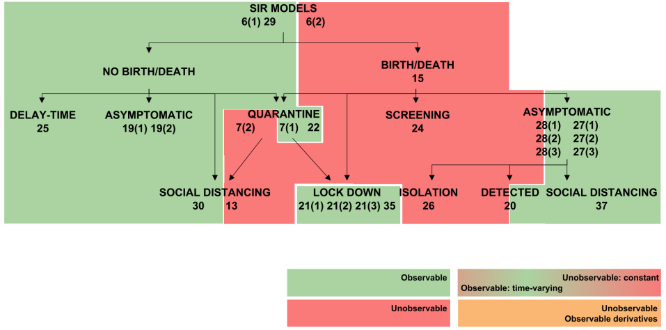
Figure 6: Identifiability of $\beta$ in SIR-models [[18]]

The IDs in the charts refer to specific models listed in tables which can be used to quickly find requirements for identifying a chosen model, or used in the model design process to ensure that the model to be used has feasible properties.

5 Observability

While identifiability is important to determine uniqueness of parameters, observability ensures that it is possible to obtain information about the states of a system. Determining the observability (and the dual controllability, which will not be covered) of states is important before considering optimal control and system identification.

5.1 Weak Local Observability

The local observability of a model can be determined using Lie derivatives of the measurement function $h(x)$ and differential equations $f(x)$ of the model. The Lie derivatives are used to form a nonlinear observability matrix for the model, which makes it possible to determine local observability.

$$\dot{x}(t) =f(x(t),u(t)), h(x) =[y_{0},y_{1},\dots,y_{N}]^{T}$$ (27)

The first Lie derivative is defined as $L_{f}^{0}h(x)=h(x)$, the next are obtained according to equation 28.

$$L_{f}^{k}h(x)=\frac{\partial}{\partial x}(L_{f}^{k-1}h(x))f(x)$$ (28)

The observability matrix contains gradient directions of the Lie derivatives and measurements $h_{i}(x)$ in $h$.

$$\mathcal{O}=\begin{bmatrix}\nabla L_{f}^{0}h_{0}&\nabla L_{f}^{1}h_{0}&\dots&\nabla L_{f}^{k}h_{0}\\ \nabla L_{f}^{0}h_{1}&\dots&\dots&\nabla L_{f}^{k}h_{1}\\ \vdots&\vdots&\vdots&\vdots\\ \nabla L_{f}^{0}h_{n-1}&\nabla L_{f}^{1}h_{n-1}&\dots&\nabla L_{f}^{k}h_{n-1}\end{bmatrix}$$ (29)

[[12]] defines a system to be locally weakly observable at a given state $x_{k}$ if $x_{k}$ is distinguishable from other states $x_{i}$ in an open neighborhood around $x_{k}$. This is fulfilled by having linear, independent rows in $\mathcal{O}$.

5.2 Weak, Local Observability in SIR-model

Using the system defined in equation.

16 with $h(x)\triangleq I$ results in the following Lie derivatives.

$$L_{f}^{0}h(x) =I$$ (30)

$$L_{f}^{1}h(x) =\beta\frac{SI}{N_{pop}}$$ (31)

Calculating $L_{f}^{2}h(x),L_{f}^{3}H(x),\dots$ results in terms containing $S$ and $I$, but not $R$. It is not possible to observe the recovered state from $I$, but it can be determined given initial condition $R(0)$.

$$\mathcal{O}=\begin{bmatrix}0&\beta\frac{I}{N_{pop}}\\ 1&\beta\frac{S}{N_{pop}}\end{bmatrix}$$ (32)

The resulting observability matrix in equation 32 remains full rank as long as $I\neq 0$, implying locally weak observability for states where a disease is present in the population.

5.3 Structural Observability

[[17], definition 3.4] defines a system to be observable if the complete differential-algebraic information of the system is contained in its system equations, making states obtainable from differential equations from the closed differential field of the system.

In simpler terms, if it is possible to ’reach’ all states $x$ of the system by time differentiating system equations (e.g. Lie derivatives on $h(x)$, equation 28) for all points in the state-space, the system is considered to be algebraically observable.

5.4 Observability of other Models

Model	Parameters	Outputs	Observability
SIR	$\alpha,\beta$	$(I,R)/(I,R,D)$	Observable
SEIR	$\alpha,\beta,\gamma$	$(I,R)$ or $(E,R)$	Observable
SEIA-$R_{I}$	$\alpha,\beta,\gamma,\mu,p$	$(I,R_{I})$ or $(E,R_{I})$	Not observable
SEIAR	$\alpha,\beta,\gamma,\mu,p$	$(I,R)$ or $(E,R)$	Observable

Table 4: Observability of epidemiological models using DAISY

Models where the population transition into ’stable’ endpoint compartments (e.g. compartment R) these have to be explicitly measured in order to observe all states. For models with infection feedback-loops (SEIR-variants) it is sufficient to measure from one of the compartment in the closed loop, in addition to the ’stable’ comparment.

For models where the population transition into separate, isolated series of compartments (asymptomatic variants) the observability is in general lost. The same way as with the EI-feedback loop the EA-feedback also require a measurement to distinguish the asymtomatic state from the infectious. In the $SEIAR$-result in table 4 this information is avaiable from compartment $R$, which is the end-state for both $I$ and $A$. When only the recovered infectious population is measured ($R_{I}$) the asymptomatic population is unobservable.

6 Bayesian Inference

With increasing availbaility of computation power, bayesian inference has become a very useful process for determining probability distributions of parameters for complex systems where analytical solutions are difficult to obtain. Bayesian inference is a process where a prior belief is updated as information becomes available, resulting in a posterior distribution.

The major advantage with Bayesian inference is that it makes it possible to obtain (probability-distributed) parameter solutions without analytically solving complex equations. The introduced SIR, SEIR and SEIAR Chain-Binomial models are examples of such models. The posterior probabilities of the infection transmission alone can become very complex after few time iterations, even for small population groups [[3]].

6.1 Bayes Rule

Following a similar notation to [[7]] the posterior distribution can be expressed in terms of Bayes rule:

$$p(x_{0:k}|y_{1:k},\theta)=\frac{p(y_{1:k}|x_{0:k},\theta)p(x_{0:k}|\theta)}{p(y_{1:k}|\theta)}\propto p(y_{1:k}|x_{0:k},\theta)p(x_{0:k}|\theta)$$ (33)

Where $x_{0:k}$ is the state trajectory, $y_{1:k}$ are observations and $\theta$ is the model parameters. For system identification the high probability regions of the posterior can be obtained by evaluating the trajectories of the system that are most probable.

6.2 Sequential Monte Carlo

Sequential Monte Carlo (SMC, also called particle filters) is used to explore the outcome space for the most probable trajectories according to a given prior distribution and likelihood function. Particles are used in differential equations to evaluate trajectory steps, and the state of the particles are used to assign individual weights. The weight of a particle describes how ’relevant’ its trajectory is to given measurements, but each step also gives an indication of how well the assigned proposal parameters $\theta_{prop}$ performs.

It is not desired to evaluate the trajectory of ’unrelevant’ particles. When the weight of particles become small compared to others they contribute less to shaping the posterior density. The following sections address this, in addition to the case where particles uniformly become too ’relevant’.

6.2.1 Importance Sampling

The posterior density $p(\theta|Y)$ is only known to proportionality (equation 33), but it is possible to approximate the statistical moments of the distribution with a sufficient number of samples. The statistical moments of the posterior can be extracted by integrating the product of posterior $p(x_{0:k}|y_{1:k},\theta)$ and a function of interest $f_{t}$.

$$\mathbb{E}[f_{k}(x_{0:k})]=\int f_{t}(x_{0:k}|\theta)p(x_{0:k}|y_{1:k},\theta)dx_{0:k}$$ (34)

One useful example of $f_{t}$ is the conditional mean $f_{t}(x_{0:t})=x_{0:t}$ which makes it possible to obtain a posterior mean using the integral. Instead of using sampling averages directly from $p(x_{k}|y_{1},\dots,y_{k},\theta)$, an importance distribution $\pi(x_{0:k},y_{1:k})$ is introduced. Equation 34 can be reformulated in terms of importance weights.

$$\mathbb{E}(f_{k}) =\frac{\int f_{t}(x_{0:k}|\theta)w_{k}(x_{0:k}|\theta)\pi(x_{0:k}|y_{1:k},\theta)dx_{0:k}}{\int w(x_{0:k}|\theta)\pi(x_{0:k}|y_{1:k},\theta)dx_{0:k}}$$ (35)

$$w(x_{0:k}|\theta) =\frac{p(x_{0:k}|\theta)}{\pi(x_{0:k}|y_{1:k},\theta)}$$ (36)

6.2.2 Sequential Importance Sampling

Importance sampling is a variance reduction technique where samples are selected with respect to a different probability distribution. The Sequential Importance Sampling (SIS) approach is one of the simplest, and can be summarized in three steps.

• Initialize with $x_{0}$, parameter proposal $\theta$ and measurements $y$.

• For each iteration: use system dynamics $f(\hat{x}_{k-1},\theta)$ to obtain state estimates $\hat{x}_{k}$. Use the likelihood of $y_{k}$ ($p(\hat{x}_{k}|y_{k})$) to assign weights to the estimates.

• Select new samples with the normalized weights as probability mass function.

The weight calculation can be written as a recursive step:

$$w_{k}\propto w_{k-1}\frac{p(y_{k}|x_{k})p(x_{k}|x_{k-1})}{\pi(x_{k}|x_{0:k-1},y_{1:k})}$$ (37)

This is a simple approach to reducing variance and exploring the probable regions of the state space. However, this approach may lead to degeneracy where all weight are assigned to few/a single particle. When degeneracy occurs most of the particles explore the same region of the state space, which is the opposite of what the particles are intended to do.

6.2.3 Sequential Importance Sampling and Resampling

Sequential Importance sampling and Resampling (SIR) solves the problem with degeneracy in SIS-resampling by introducing a measure for the effective number of particles:

$$N_{eff}=\frac{1}{\sum_{i=1}^{N_{p}}(w_{k}^{(i)})^{2}}$$ (38)

Where $N_{p}$ is the total number of particles. If $N_{eff}$ falls below a given threshold, the particles are resampled according to their current weights, followed by all weights being set uniformly to $\frac{1}{N_{p}}$.

6.3 Markov-Chain Monte Carlo

Markov-Chain Monte Carol (MCMC) is a widely used approach for estimating model parameters for systems where true states are not directly observable, but obtainable from probability distributed variables. The method applies Sequential Monte Carlo simulations to Markov models in order to determine the posterior probability distribution of the parameters to be identified.

6.3.1 Metropolis Algorithm

When a trajectory with weights has been computed (section 6.2.2) the weights can be used to evaluate if the proposed parameters $\theta_{i}$ were better or worse than the previous proposal $\theta_{i-1}$. The Metropolis algorithm is one of many solutions for determining the sequence of parameters to evaluate, and is applied and evaluated over multiple trajectories.

Data: $\theta_{i}=\theta_{0}$ where $p(\theta_{0}|y)>0$, $N_{\theta}$

for i in $N_{\theta}$ do

       Evaluate trajectory for $\theta_{i}$

       Retrieve the average weight $\frac{\sum_{k=1}^{N_{t}}p(\hat{x}_{k}|y_{k})}{N_{t}}\approx p(\theta_{i}|y)$

       Calculate $\alpha=\min(1,\frac{p(\theta_{i}|y)}{p(\theta_{i-1}|y)})$

       if Uniform$(0,1)>\alpha$ and $\theta_{i}\neq\theta_{0}$ then

             draw $\theta_{i+1}$ from the symmetric distribution $J(\theta_{i+1}|\theta_{i-1})$

       end if

      else

            draw $\theta_{i+1}$ from the symmetric distribution $J(\theta_{i+1}|\theta_{i})$

       end if

      

end for

Algorithm 1 SMC with Metropolis Algorithm

The Metropolis algorithm works only for symmetric proposal distributions $J$.

6.3.2 Metropolis-Hastings

To balance out the likelihood ratio $\alpha$ (algorithm 1) with respect to the asymmetry of $J$, the likelihoods are corrected using proposal distribution $J$ (equation 39)

$$\alpha=\frac{\frac{p(\theta_{i}|y)}{J(\theta_{i}|\theta_{i-1})}}{\frac{p(\theta_{i-1}|y)}{J(\theta_{i-1}|\theta_{i})}}$$ (39)

The use of asymmetric proposal distributions can improve parameter proposals and make the algorithm find high parameter likelihoods faster. Given that the parameter proposals sufficiently explore the parameter space, the empirical distribution of saved parameters $\theta_{0},\dots,\theta_{N}$ will converge to the true parameter distribution.

6.4 Implementations: PyMC3

SMC and MCMC-algorithms can require a lot of evaluations in order to produce good posterior densities. This makes it important to choose a language which supports fast distribution sampling. Along with simpler, custom implementations of MCMC and SMC, libraries in both Python and C++ have been considered.

PyMC3 [[25]] is a library in Python for bayesian statistical modeling in general, and supports the use of SMC and MCMC-samplers. The samplers have been able to evaluate model dynamics effectively through the use of Theano, a library which uses an optimizing compiler to translate algebraic expressions to code efficiently, with the addition of GPU-support.

The development of Theano was officially ended in 2018 but forked and to some extent maintained by the pyMC-team. A substantial effort was made in order to setup and use the pyMC3 interface for this project, which eventually succeeded for one specific version of Python (3.8) on Ubuntu, but no solution was found compatible for Windows.

The pyMC3 application interface provides good solutions for continous ODEs and Markov chains with state-invariant transition-distributions, but did not support binomial sampling for ODEs directly. An attempt was made at solving the issue by constructing a black-box Theano model, but this breaks the intended abstraction of the library, and did not result in good performance either.

6.5 A Custom SMC/MCMC-Library

In order to remove the abstraction and get an interface able to utilize hardware better, a SMC-library called Sequential Monte Carlo Template Class [[13]] was redesigned. The library takes advantage of the templating function in C++ in order to generate code for a sampler fitted to a custom particle class, with custom system dynamics and probability densities.

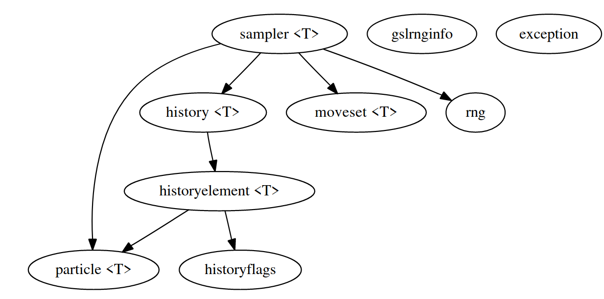
Figure 7: SMCTC Collaboration Chart[[13]]

The library depends on the GSL-library[[8]] for random number generation, which samples substantially faster than Python’s NumPy and SciPy implementations.

6.5.1 Overview

The custom implementation makes use of some features from the sampler, rng and particle classes, but is modularized differently in order to clearly separate between data storage and routines.

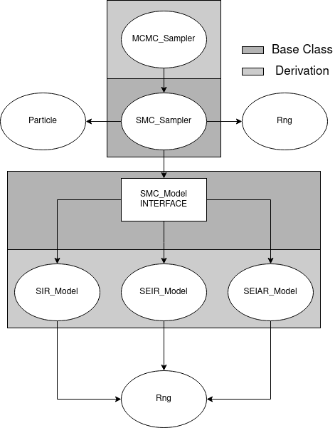
Figure 8: Collaboration chart for custom MCMC-library

6.5.2 Interface

An interface class SMC_Model.hh is implemented to limit the interaction between the SMC/MCMC-sampler and the custom model implementation. The following virtual functions listed in the class needs to be implemented by the user:

void Init(double* &, long &)

Allocate space needed and initialize state.

void Step(const long &lTime, double* X, const double *param)

Move the particle state to the next timestep.

void ProposalSample(const double* oldParam, double* result)

Draw a new parameter proposal from a custom distribution.

double LogLikelihood(const double *X, const long &lTime)

Evaluate likelihood for the current timestep using current estimate $X$ and the observation data.

void Reset(double* X)

Reset state values in order to prepare for a new SMC-trajectory evaluation.

6.5.3 SMC Sampler

The SMC-sampler sequentially pass particle states and weights to the model, and afterwards perform resampling. Its workflow can be briefly summarized in a few declarations:

void InitializeParticles()

Initializes the state and weight of all particles.

void MoveParticles()

Moves all particles to the next timestep.

double GetESS()

Calculate the current Effective Sample Size.

void Resample(ResampleType lMode)

Performs resampling using the current particle weights, with support for multiple resampling strategies.

void Normalize_Accumulate_Weights()

Accumulates the weights throughout the SMC-run, and normalizes the weights to sensible values for importance and resampling.

void ResetParticles()

Set state and weights of each particle back to initial.

6.5.4 MCMC Sampler

The MCMC-sampler controls the SMC-iterations and keeps track of the used parameters and accumulated weights. It can either be constructed independently, or built on top of an SMC sampler using a copy constructor.

void IterateMCMC()

Runs SMC sampler iterations until it has reached end of trajectory. Afterwards Metropolis() is called to propose a new parameter, followed by a particle reset.

int Metropolis(void)

Runs Metropolis algorithm (section 6.3.1) with current and previous weights and parameters.

Note: Only symmetric proposal distributions have been used in this project. Metropolis-Hastings requires a small extension to the interface and MCMC_Sampler classes, but can easily be added when needed.

6.5.5 Comparison of Performance

The stochastic trajectory simulations in Python were timed to use an average of $\approx 0.135s$ per SIR trajectory when evaluating beta-binomial distributions with the Scipy library. The custom MCMC-implementation was measured to evaluate 100 particle trajectories with resampling and weight updates in $\approx 5\pm 1ms$.

6.6 Simulation Setup

Given a list of measured infections and an initial state, there are many parameter sets $\theta$ for the stochastic SIR, SEIR and SEIAR models which are able to produce the same results. This section presents a method to sample from the epidemiological Chain-Binomial models, which will be applied on measurements generated by the following deterministic models.

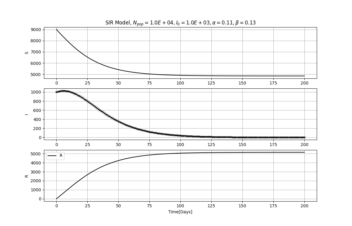
Figure 9: Deterministic SIR-trajectory for measurements

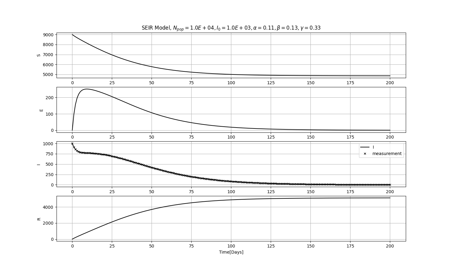
Figure 10: Deterministic SEIR-trajectory for measurements

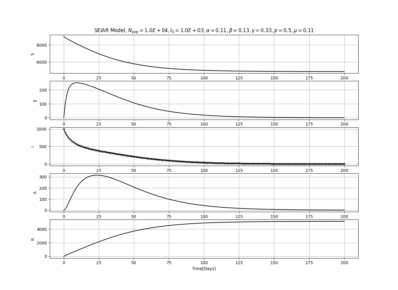
Figure 11: Deterministic SEIAR-trajectory for measurements

The identification algorithm presented in this section will be given the initial conditions $x_{0}$, total population $N_{pop}$ and step size $\Delta t$, in order to evaluate which parameter set $\hat{\theta}$ that is most likely to reproduce the given measurements using a stochastic model. Initial parameter proposal $\theta_{prop,0}$ will be set to $2\theta$ (Where $\theta$ is the true, deterministic parameter set, and with the exception of parameter $p$, which is set to $1.5p_{true}$).

6.7 Simulation Results

Running the implemented MCMC algorithm with the stochastic SIR-model, 100 particles, 50000 iterations, $p(x|\theta,y)=\mathscr{N}(x;\sigma=100)$ and proposal parameter $\theta_{prop,k}\sim\mathscr{N}(\theta_{k-1},\begin{bmatrix}0.1\alpha&0.1\beta\end{bmatrix}\cdot I)\in[0,\infty)$ results in the following parameter distributions:

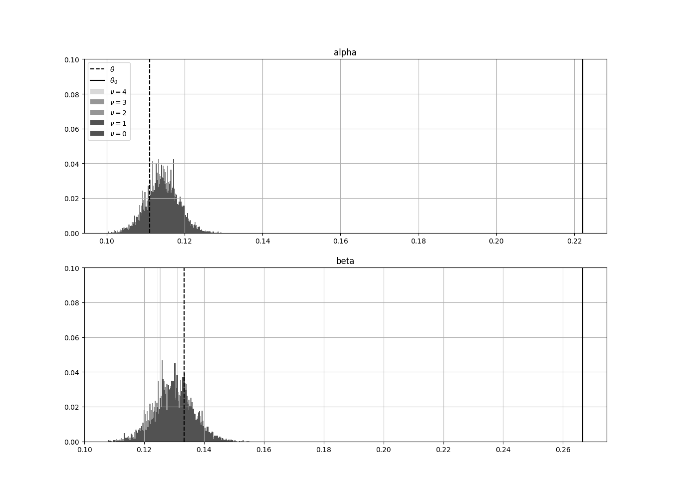
Figure 12: Parameter distributions for Stochastic SIR-Model using implemented C++ MCMC-library.

Running the implemented MCMC algorithm with the stochastic SEIR-model, 100 particles, 50000 iterations and $p(x|\theta,y)=\mathscr{N}(x;\sigma=100)$ resulted in the following parameter distributions:

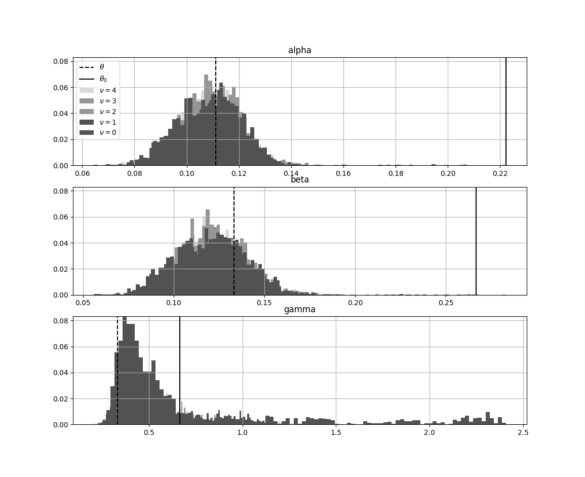
Figure 13: Parameter distributions for Stochastic SEIR-Model using implemented C++ MCMC-library.

Running the implemented MCMC algorithm with the stochastic SEIAR-model, 100 particles, 50000 iterations and $p(x|\theta,y)=\mathscr{N}(x;\sigma=100)$ resulted in the following parameter distributions:

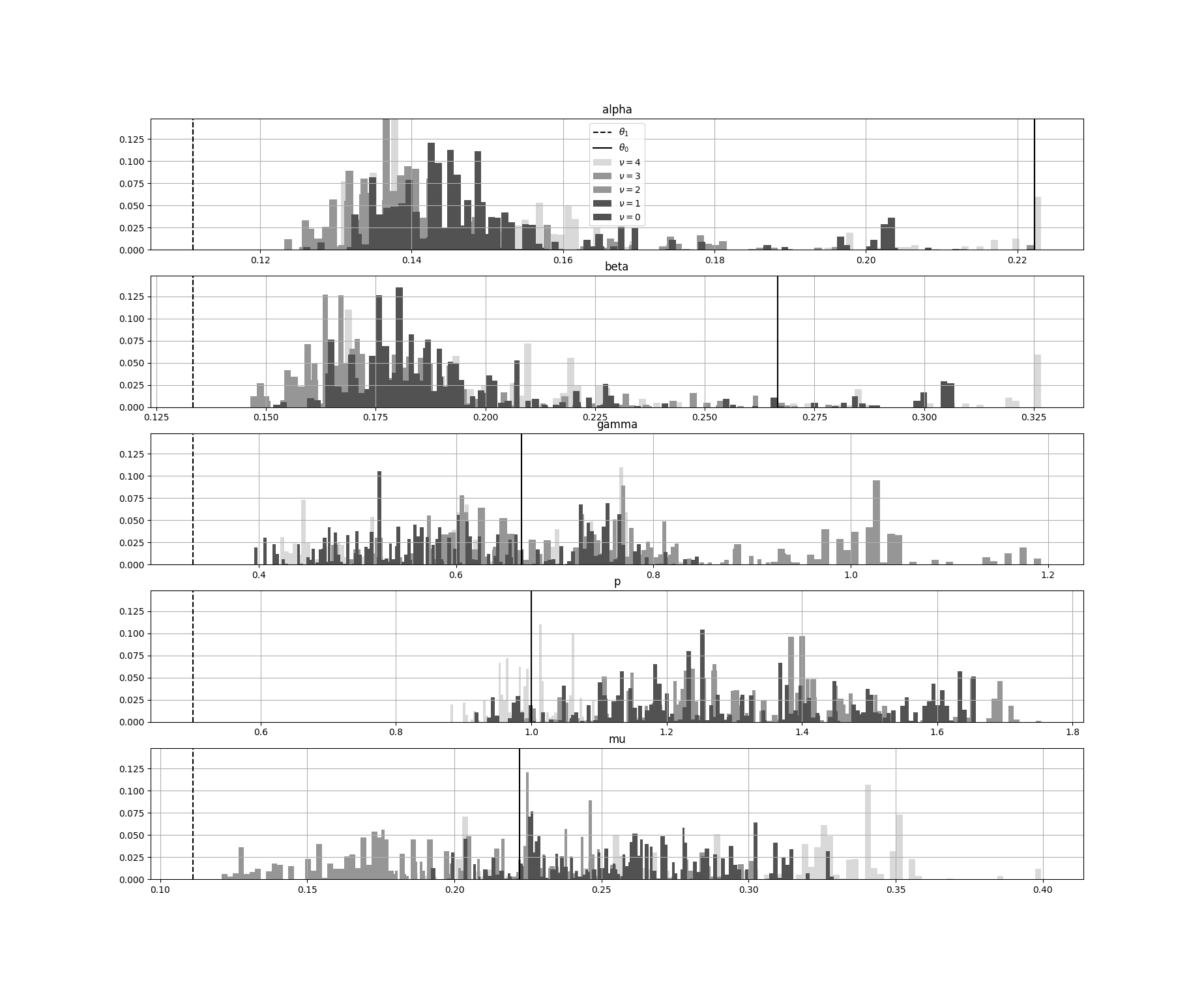
Figure 14: Parameter distribution for Stochastic SEIAR-Model using implemented C++ MCMC-library.

6.8 Remarks on the Simulations

There are many possibilities for parameter tuning within SMC/MCMC, where some give good convergence to a true solution, and others lead to no convergence at all. In this project, the algorithm has been tuned from intuitions, which may be impossible for more complex models.

$p(x_{0:k}|\theta,y_{1:k})$ was tuned to sufficiently distinguish a bad infection count prediction from a good one, in the sense that a ’good’ stochastic model has the tendency to estimate within one standard deviation $\sigma$ of $y_{1:k}$. Reducing $\sigma$ could speed up convergence locally (which was not prioritized, given the 50000 iterations used) at the cost slowing down convergence when $\theta_{0}$ is far from $\theta$.

Different magnitudes was used for the standard deviation of $\theta_{prop,k}$. Using a large deviation resulted in an increase in Metropolis rejections, since the parameters proposed gave radical trajectories. Using a very small deviation did not ensure a consistent convergence either. Because of the randomness from the stochastic models, an accepted small parameter step do not neccesarily have to be a step in the right direction.

6.9 Discussion

The implemented MCMC-library managed to identify a reasonable estimate for the parameter for the stochastic SIR and SEIR models. The parameter distributions in figures 12, 13 are mostly normally distributed with an offset from the true deterministic parameters.

The stochastic model require a different parameterization than the deterministic for this population size. This is relatable to the simulated trajectories in section 3 which show that parameterization at this population size makes the stochastic models behave slightly different than the deterministic ones.

An increase in $\nu$ did not have a significant impact on the parameter distributions. There are many dependencies in parameterization here, which makes it difficult to determine if this is a valid result. The population size is moderately large ($N_{pop}=10000)$ and homogenous, which according to results from section 3 indicates that $\nu$ should have a small impact on the trajectory. This is consistent with the current result. On the other hand, the moderately large standard deviation $\sigma=100$ could have slowed down the convergence towards the true estimate, but 50000 iterations should counteract the impact of this.

7 Future Work

7.1 Networked Mean Field Approximations

As mentioned in the introduction it is desired to associate the deterministic to the stochastic nature of true epidemics. While Chain-Binomials are able to capture initial outbreaks, they do not use the spatial information required to do accurate predictions.

Instead of modelling initial outbreaks with Chain-Binomials [[5]] use deterministic, networked mean-field approximations ([[20]]) to approximate a network with multiple compartmental models.

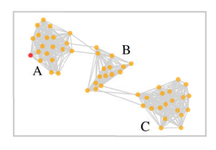
Figure 15: Network subject to mean-field approximations [[5]]

Finding good approximations for network clusters, possibly with confidence intervals, would be a step in the right direction, and may be necessary in order to apply optimal control on smaller populations. The results from [[5]] show that optimal control with three deterministic approximation for the given network outperforms the alternative choices.

If the custom MCMC-implementation could be improved to be computationally efficient for network models, it could further be possible to use spatial infection measurements to infer posterior parameter distributions for deterministic SIR/SEIR/SEIAR models.

Local solutions for the deterministic models have already been studied, and are attainable through the use of multiple shooting methods and Interior-Point Optimization (IPOPT) [[26]]. This sort of optimization could possibly extended to account for multiple compartmental models, resulting in a robust strategy which integrates spatial information, while still being able to retain anayltical properties in the model.

7.2 Practical Identifiability and Dynamic Observability

While structural observability and idenitifiability describes the uniqueness of states and parameters, it does not necessarily hold when the models are subject to noise. In this case it may be a need for a continous quantification of identifiability and observability, which is addressed respectively in [[22]], [[2]].

7.3 MCMC Parameterization and Correlation

There are many aspects to be explored within parameterization of the SMC/MCMC-algorithms. Effective sample size $N_{eff}$, the number of SMC-particles and the previously mentioned distributions give many options, and this only covers the methods of standard SIR-resampling and parameter choices with Metropolis. There are many SMC and MCMC-methods to explore, some of them are mentionable.

• Hamiltonian MCMC - Models the parameters as a particle, which conserves potential/kinetic energy as it travels through the parameter space, where the energy distribution is determined by the measurement likelihood.

• Gibbs Sampling - A frequently used special case of Metropolis Hastings.

• In addition to standard resampling, the SMCTC-library implemented Residual, Stratified and Systematic resampling strategies.

Using old parameters to propose new ones naturally leads to correlated decisions in the MCMC-sampler. Due to the sample size, this was negligible for the project simulations, but its impact should be studied for future projects.

7.4 Optimal Control on NTNUs COVID-19 Model

The model implemented by the NTNU COVID-19 Taskforce use the following model/control scheme:

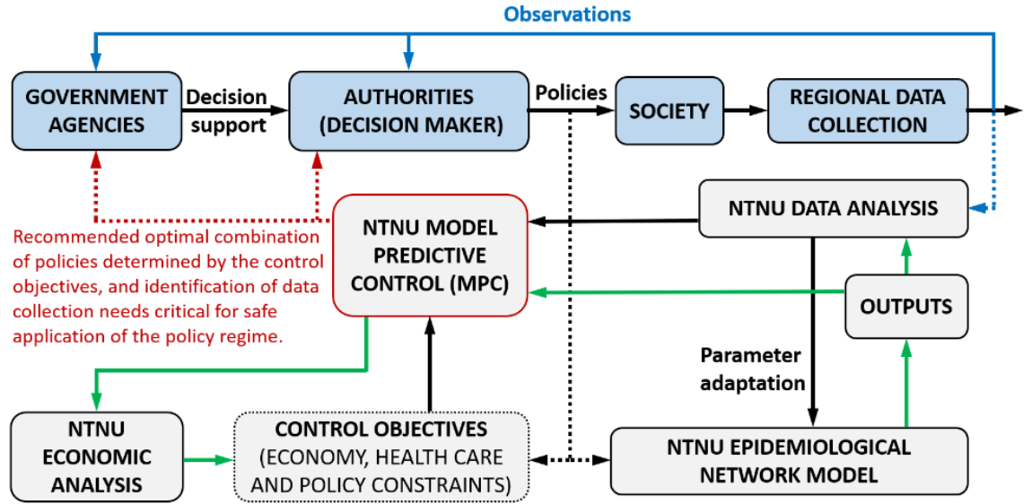
Figure 16: Block Diagram for the NTNU COVID-19 Modeling and Control scheme [[6]]

The current Model Predictive Control (MPC) use the deterministic SEIR model as approximation for the underlying network model. However, if the network consists of many clusters (figure 15) it would be better approximated with multiple SEIR-models. Using SMC and MCMC to find parameter distributions for multiple models can lead to a more accurate and robust control strategy.

8 Conclusion

A variety of probability distributions have been studied in this project, providing ways of representing overdispersion in Chain-Binomial models. Onwards, the overdispersed distributions has been used to illustrate how trajectories change in epidemiological models, which resulted in a moderately weak impact given a total population size of $N_{pop}>10000$.

Trajectory simulations show that Chain-Binomials are important for modeling non-homogenous small populations, while it is possible to approximate them with deterministic models for homogenous, large populations. These simulations do show indicative trends, but a larger sample size may be needed to approximate true confidence intervals.

The structural identifiability of the SIR, SEIR and SEIAR models was found in different configurations using DAISY. While parameters in SIR and SEIR are identifiable, additional measures are needed in order to retrieve parameters in models with asymptomatic compartments.

The structural observability of the SIR, SEIR and SEIAR models was assessed in different configurations, revealing that the asymptomatic compartment is structurally unobservable, while the SIR and SEIR models are structurally observable.

The Sequential Monte Carlo and Markov Chain Monte Carlo methods were studied to find ways of estimating parameter distributions for Chain Binomial models. This resulted in a computationally efficient implementation which successfully converges towards true parameters, given a good parameterization. The exception was the unobservable SEIAR model, which did not converge towards the true parameter values.

Overall, the project has been a good introduction to clarify what kind of information that is retrievable from the simplest epidemiological models, and it has presented ways of modelling unavailable information in terms of uncertainty, and it has provided an identification algorithm that can be applied to more complex models.

Appendix

A Buchberger Algorithm

Denoting $LM(p)$ as the leader mononial and $LT(p)$ as the leader term of polynomial $p$ ,and $LCM(p,q)$ the least common multiple of polynomials $p,q$, S-polynomials (Subtraction) can be defined:

$$S(p,q)=\frac{LCM(LM(p),LM(q))}{LT(p)}\cdot p-\frac{LCM(LM(p),LM(q))}{LT(q)}\cdot q$$ (40)

Data: Input basis $f=\{f_{1},\dots,f_{N}\}$

g:= f while g $\neq$ h do

       h := g for all pairs $(p,q),p\neq q,p,q\in g$ do

             $S$:=$S(p,q)$

             $r$:=remainder(S, g)

             if $r\neq 0$ then

                   add $r$ to basis $g$

             end if

            

       end for

      

end while

Algorithm 2 Buchberger Algorithm

Appendix A Code Overview

Working examples for the MCMC are frozen on the ”Inspera” branch of a git repository:

git clone https://github.com/jonasbhjulstad/MCMC.git

The project is structured with the following top-level folders:

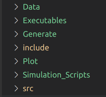
Figure 17: Top-level folders of C++ project

Note: The file storage paths must be updated in order to direct the parameter/weight output to correct filepaths.

• Data - Stores parameters, weights and generated trajectories

• Executables - Contains the compiled binaries. (run_SXXX, gen_XXX)

• Generate - Contains source files for generating trajectories

• Plot - Contains .py-files for trajectory and parameter plots

• Simulation_Scripts - Contains One main parameter configuration file, and separate execution loops for the models.

• src - Contains source code files

References

- [1] Helen Abbey “An examination of the Reed-Frost theory of epidemics” In Human biology 24.3 Johns Hopkins Press, 1952, pp. 201
- [2] Portes LL Aguirre LA “Structural, dynamical and symbolic observability: From dynamical systems to networks” URL: https://doi.org/10.1371/journal.pone.0206180
- [3] Becker “A general chain binomial model for infectious diseases”, 1981
- [4] Giuseppina Bellu, Maria Pia Saccomani, Stefania Audoly and Leontina D’Angiò “DAISY: A new software tool to test global identifiability of biological and physiological systems” In Computer Methods and Programs in Biomedicine 88.1, 2007, pp. 52–61 DOI: https://doi.org/10.1016/j.cmpb.2007.07.002
- [5] E.H. Bussell, C.E. Dangerfield, C.A. Gilligan and N.J. Cunniffe “Applying optimal control theory to complex epidemiological models to inform real-world disease management” In bioRxiv Cold Spring Harbor Laboratory, 2018 DOI: 10.1101/405746
- [6] COVID-Taskforce “Description of modelling framework per April 29, 2020”, 2020
- [7] Gordon Doucet A. “An Introduction to Sequential Monte Carlo Methods”, 2001 URL: https://doi.org/10.1007/978-1-4757-3437-9˙1
- [8] M. Galassi “GNU Scientific Library Reference Manual (3rd Ed.)” URL: http://www.gnu.org/software/gsl/
- [9] William Heaton Hamer “The milroy lectures on epidemic diseases in england: The evidence of variability and of persistency of type; delivered before the royal college of physicians of london, march 1st, 6th, and 8th, 1906” Bedford Press, 1906
- [10] Sha He, Sanyi Tang and Libin Rong “A discrete stochastic model of the COVID-19 outbreak: Forecast and control” In Mathematical Biosciences and Engineering 17, 2020, pp. 2792–2804 DOI: 10.3934/mbe.2020153
- [11] Anthony C. Hearn “REDUCE”, 2019 URL: https://reduce-algebra.sourceforge.io/
- [12] R. Hermann and A. Krener “Nonlinear controllability and observability” In IEEE Transactions on Automatic Control 22.5, 1977, pp. 728–740 DOI: 10.1109/TAC.1977.1101601
- [13] Adam M. Johansen “SMCTC: Sequential Monte Carlo in C++” In Journal of Statistical Software, Articles 30.6, 2009, pp. 1–41 DOI: 10.18637/jss.v030.i06
- [14] William Ogilvy Kermack and Anderson G McKendrick “A contribution to the mathematical theory of epidemics” In Proceedings of the royal society of london. Series A, Containing papers of a mathematical and physical character 115.772 The Royal Society London, 1927, pp. 700–721
- [15] J. Köhler et al. “Robust and optimal predictive control of the COVID-19 outbreak”, 2020 arXiv:2005.03580 [q-bio.PE]
- [16] Stephen Lauer “The Incubation Period of Coronavirus Disease 2019 (COVID-19) From Publicly Reported Confirmed Cases: Estimation and Application” PMID: 32150748 In Annals of Internal Medicine 172.9, 2020, pp. 577–582 DOI: 10.7326/M20-0504
- [17] Rafael Martínez-Guerra and Christopher Diego Cruz-Ancona “Algebraic Observability for Nonlinear Systems” In Algorithms of Estimation for Nonlinear Systems: A Differential and Algebraic Viewpoint Cham: Springer International Publishing, 2017, pp. 15–24 DOI: 10.1007/978-3-319-53040-6˙3
- [18] Gemma Massonis, Julio R. Banga and Alejandro F. Villaverde “Structural Identifiability and Observability of Compartmental Models of the COVID-19 Pandemic”, 2020 arXiv:2006.14295 [q-bio.PE]
- [19] Marcelo Menezes Morato, Igor Pataro, Marcus Americano da Costa and Julio Normey-Rico “A Parametrized Nonlinear Predictive Control Strategy for Relaxing COVID-19 Social Distancing Measures in Brazil”, 2020
- [20] Cameron Nowzari, Victor M. Preciado and George J. Pappas “Analysis and Control of Epidemics: A survey of spreading processes on complex networks”, 2015 arXiv:1505.00768 [math.OC]
- [21] L.. Olivier, S. Botha and I.. Craig “Optimized Lockdown Strategies for Curbing the Spread of COVID-19: A South African Case Study” In IEEE Access 8, 2020, pp. 205755–205765 DOI: 10.1109/ACCESS.2020.3037415
- [22] A. Raue et al. “Structural and practical identifiability analysis of partially observed dynamical models by exploiting the profile likelihood” In Bioinformatics 25.15, 2009, pp. 1923–1929 DOI: 10.1093/bioinformatics/btp358
- [23] P Erdős-A Rényi and P Erdos “On the evolution of random graphs” In Publ. Math. Inst. Hung. Acad. Sci. A 5, 1960, pp. 17–61
- [24] J.F. Ritt “Differential Algebra”, Colloquium publications American Mathematical Society, 1950 URL: https://books.google.no/books?id=vBpzMqTH1j4C
- [25] Salvatier “Probabilistic programming in Python using PyMC3”, 2016
- [26] Andreas Wächter and Lorenz T. Biegler “On the implementation of an interior-point filter line-search algorithm for large-scale nonlinear programming” In Mathematical Programming 106.1, 2006, pp. 25–57 DOI: 10.1007/s10107-004-0559-y
- [27] Sean L. Wu et al. “Substantial underestimation of SARS-CoV-2 infection in the United States due to incomplete testing and imperfect test accuracy” In medRxiv Cold Spring Harbor Laboratory Press, 2020 DOI: 10.1101/2020.05.12.20091744