Signatures of gravitational wave memory in the radiative process of entangled quantum probes
Abstract
In this article, we examine entangled quantum probes in geodesic trajectories in a background with gravitational wave (GW) burst. In particular, these quantum probes are prepared initially either in the symmetric or anti-symmetric Bell’s states and we study the radiative process as the GW burst passes. Our considered GW burst backgrounds have the profiles of – Heaviside-theta, , Gaussian, and -squared functions respectively. The first two burst profiles have an asymmetric nature and thus result in non-zero gravitational wave memory. Whereas, for the last two symmetric profiles there is no asymptotic memory. For eternal switching, our observations suggest that the collective transition rate for the entangled probes due to symmetric GW bursts remains the same as obtained in the flat space. Whereas, for asymmetric bursts with memory, there is a finite change, indicating a direct possibility to distinguish between the two above-mentioned scenarios. We also consider finite switching in terms of Gaussian functions and observe characteristic differences in the radiative process between the GW backgrounds with and without memory. Notably, if the Gaussian switching is peaked much later compared to the passing of GW, only memory profiles contribute to the radiative process. We further discuss the physical implications of our findings.
I Introduction
The utilization of quantum field theory in curved spacetime results in outcomes that were unforeseen in classical general relativity (GR). One of the most celebrated of such outcomes is the Hawking effect, which predicts a thermal distribution of particles emitted from a black hole event horizon, as observed by an outside observer, see hawking1975 . Another subsequent interesting development is in the form of the Unruh effect Unruh:1976db , where the Minkowski vacuum is seen populated by a thermal distribution of particles when observed from an accelerated frame. These effects are often regarded as a gateway to peek into the quantum features in a GR background book:Birrell ; Don_Page:2004 . Over the years, there have been several efforts to detect these effects, see Martin-Martinez:2010 ; Aspachs:2010 ; Rideout:2012 ; Stargen:2021 (for an exhaustive list see Crispino:2007eb and the references therein). One of the most dedicated approaches in this line of investigation has been in the domain of analogue gravity, see Rodriguez-Laguna:2016 ; Blencowe:2020 ; Gooding:2020 ; Biermann:2020 ; Onoe:2021 ; Hu:2018_nature . However, as analogue gravity models lack the interpretation of curvature, they are often unable to provide a complete understanding of the intricacies related to a general curved background.
Another promising avenue to investigate such features of semiclassical gravity has been in the field of relativistic quantum information (RQI), see Reznik:2002fz ; Floreanini:2004 ; FuentesSchuller:2004xp ; Ball:2005xa ; Cliche:2009fma ; Lin:2010zzb ; MartinMartinez:2012sg ; Salton:2014jaa ; Martin-Martinez:2015qwa ; Zhou:2017axh ; Cai:2018xuo ; Pan:2020tzf ; Barman:2021oum ; K:2023oon ; Hsiang:2024qou for its different aspects. Several set-ups in the domain of RQI involve employing entangled quantum systems for studying the entanglement due to motion Koga:2018the ; Koga:2019fqh ; Zhang:2020xvo ; Barman:2022xht , background geometries FuentesSchuller:2004xp ; Cliche:2010fi ; MartinMartinez:2012sg ; Kukita:2017etu ; Barman:2021kwg ; Barman:2023rhd ; Xu:2020pbj ; Gray:2021dfk ; K:2023oon , thermal bath Brown:2013kia ; Simidzija:2018ddw ; Barman:2021bbw , etc. A relatively underexplored though interesting area of research in RQI has been the study of radiative process of entangled detectors. Inspired by the light-matter interaction in atomic systems as introduced by Dicke Dicke:1954 , these works study the dynamics of entangled detectors and their dependence on various system parameters. Earlier works on the radiative process with static entangled detectors in flat spacetime have shown that the collective transitions are significantly different compared to single detector case and can get enhanced or reduced depending on the initial entangled state Arias:2015moa ; FICEK2002369 . At the same time, entangled detectors in uniform acceleration and in contact with a thermal bath exhibit anti-Unruh-like effects, see Barman:2021oum . The radiative process of entangled detectors is also studied in other configurations, such as for detectors in circular trajectories Picanco:2020api ; Barman:2022utm , and in different black hole and cosmological spacetimes Menezes:2017oeb ; Cai:2017jan ; Liu:2018zod .
In this work, we consider a system comprising of gravitational wave (GW) bursts passing through a flat background and investigate the radiative process of entangled detectors that are in geodesic trajectories. In recent times, the investigation of entanglement in gravitational wave backgrounds have received significant interest Xu:2020pbj ; Gray:2021dfk ; Chiou:2016exd ; Barman:2023aqk ; Wu:2024qhd . For instance, the authors in Barman:2023aqk have studied how spacetimes having gravitational wave (GW) bursts with and without memory control the concurrence measure of the harvested entanglement. GW memory refers to the permanent shift in the position of test particles upon the passage of a GW pulse Favata:2010 ; Chakraborty_EPJP:2022 ; Chakraborty:2021 . The change in the geodesic separation () is related to the change in GW metric perturbation () as:
| (1) |
This non-zero permanent change indicates the GW memory effect, see Tolish:2014bka ; maggiore2007gravitational . In case of burst with (without) memory, the asymptotic GW strain at past and future times are different (same) Barman:2023aqk . Phenomenological models considering bursts with memory can be found in gravitational bremsstrahlung in hyperbolic orbits Kovacs:1978 ; Garcia-Bellido:2017 ; Hait:2022 , core-collapse supernova Mukhopadhyay:2021 ; Hait:2022 , and gamma-ray bursts Sago:2004 . In our present work, we consider both GW bursts with and without memory propagating over Minkowski spacetime to investigate the radiative process. The detectors in this scenario are considered to be the two-level atomic Unruh-DeWitt detectors. Our aim is to understand how GW memory controls the transitions between the two collective energy levels of entangled detectors. It is to be noted all previous works investigating entanglement in a GW background worked with static detectors. In the present article, we consider detectors in geodesic trajectories which are initially prepared in an entangled state. To be specific, they are prepared either in the symmetric or in the anti-symmetric Bell states.
In this work, we consider both the eternal and finite switching between the detectors and the scalar field, where the finite switching is controlled by a Gaussian function. Both the eternal and the finite switching have their own significance. For instance, eternal switchings are free of any transient effects and can bring out features that are specific to the background spacetime or the detector motion. On the other hand, finite switching is relevant from the experimental point of view, as one cannot construct a practical experimental set-up with detectors that interact for an infinite time with the background field. In particular, from our analysis, the key observation is that the GW profiles with memory (), i.e., the Heaviside theta and profiles, give a non-vanishing contribution in the radiative process for eternal switching. On the other hand, with finite switching both the symmetric and asymmetric bursts can have nonzero contribution in the radiative process. However, with the latter switching, the memory bursts will always provide some finite contribution if the detectors are switched on during or after the passing of the GW. Whereas, for the symmetric bursts () the non-zero finite contribution is observed only during the passing of the GW, and the contribution vanishes much after the GW has passed. We discuss the physical implications of our findings and emphasize on the future prospects of experimental realizations.
The manuscript is organized in the following manner. In Sec. II we briefly discuss the model set-up for studying the radiative process of entangled Unruh-DeWitt detectors. In this section, we also introduce the GW burst background and elucidate the detector trajectories, which are geodesics in the considered background. In Sec. III we recall the expressions of the scalar field mode solutions in a GW background and estimate the expressions of the Green’s function corresponding to the considered detector trajectories. Subsequently, in Sec. IV we utilize these Green’s functions to obtain different transition coefficients corresponding to the radiative process and also estimate the total transition probability for specific transitions in the infinite interaction (eternal switching) scenario. Whereas, in section V we consider the Gaussian switching scenario and find the transition coefficients and the total transition probabilities. In Sec. VI we present our key observations, discuss the implication of our findings.
II Set-up and detector trajectories
In this section, we outline the model setup for the radiative process of two entangled quantum probes. We also discern the geodesic trajectories to be followed by these probes in the GW burst background. We shall observe that the collective transition of the entangled quantum probes not only depends on the individual detector Wightman functions but also on the Wightman function corresponding to the geodesic distance between two different detectors. Therefore, it is natural to believe that the effect of GW memory in these trajectories and the subsequent distortions in it should also get reflected in the collective transition of the entangled probes.
II.1 Model set-up
We start with a brief discussion on the set-up for the radiative process of entangled quantum probes. In this regard, we consider two entangled detectors in a background spacetime interacting with a massless, minimally coupled scalar field . The set-up is inspired by the works on light-matter interaction by Dicke (see Dicke:1954 for the original discussion and Rodriguez-Camargo:2016fbq for a recent one). In recent times, the set-up has been used in various scenarios and for different detector motions, see Arias:2015moa ; Rodriguez-Camargo:2016fbq ; Costa:2020aqa ; Barman:2021oum ; Barman:2022utm . In particular, we consider the entangled quantum probes to be modelled after two-level, point-like, atomic detectors, popularly known as the Unruh-DeWitt detectors. These detectors were initially conceptualized to understand the Unruh and the Hawking effects (see Unruh:1976db ; hawking1975 on the conceptions of these effects), but in recent times have become ubiquitous in understanding entanglement phenomenon in curved spacetime, see Xu:2020pbj ; Barman:2021oum ; Barman:2022utm ; Barman:2023aqk . Let us provide an outline for the set-up in which the complete system Hamiltonian is of the form
| (2) |
where denotes the free detector Hamiltonian, is the free scalar field Hamiltonian, and corresponds to the interaction between the detectors and the scalar field. The free detector Hamiltonian describing two static atoms, see Dicke:1954 , can be expressed as
| (3) |
In this expression , with , is the energy operator for the detectors, and it is defined as
| (4) |
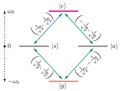
where and respectively denote the ground and excited states of the - atomic detector. In Eq. (3), denotes the identity operator and the energy gap between different energy levels of the collective two detector system. As pointed out in Arias:2015moa , for two identical and static detectors the energy eigenstates and eigenvalues for the collective detector system can be expressed as
| (5a) | |||||
| (5b) | |||||
| (5c) | |||||
| (5d) | |||||
where and denote the ground and the excited states of the collective system. Whereas and are the degenerate maximally entangled Bell states also known as the symmetric and anti-symmetric Bell states. We have provided a pictorial representation of these states, energy levels, and the possible transitions between them in Fig. 1.
The interaction between the detectors and the field is assumed to be of monopole type and the interaction Hamiltonian is explicitly expressed as
| (6) |
where we have considered the interaction strength to be same for both the detectors. While and respectively denote the monopole operators and the switching function corresponding to the interaction. In particular, for detector the monopole moment operator is given by
| (7) |
In the interaction picture, utilizing the previously mentioned interaction Hamiltonian the time evolution operator can be expressed as
| (8) |
where signifies the consideration of time ordering. Moreover, we consider the initial and final collective detector states to be and respectively. Then treating the interaction strength perturbatively one obtains the transition probability
| (9) |
where , is the energy gap between the states and with energies and . While denotes the expectation value of the monopole moment operator. One can use the expression of the monopole moment operator from Eq. (7) to obtain these expectation values between different collective detector states. For instance, one can easily obtain for states and the expectation values . Therefore, these transitions are not permissible. On the other hand, the other expectation values are and . Similarly, with the Bell states and the ground state the expectation values are and . These expectation values of the monopole moment operators are also depicted in Fig. 1.
In Eq. (9) the most important part that contains the information about the background and the detector trajectories are . Following Barman:2022utm , we refer different components of as the auto or the cross-transition probabilities, depending on whether that component correspond to a single detector or correlates two different ones. The explicit form of this quantity is given by
| (10) | |||||
where the denotes the positive frequency Wightman function evaluated along the detector trajectories and is defined as
| (11) |
where denotes a suitable field vacuum state. Our main aim in the subsequent sections is to evaluate these Wightman functions for detectors in geodesic trajectories in a GW background and then use them in discerning the transition probabilities of Eq. (9) for transitions from the symmetric and anti-symmetric Bell’s states to the collective ground/excited state.
In our main analysis, we are going to consider two types of switching, namely the eternal switching with and finite switching in terms of Gaussian function . In those scenarios, we define the transition probability rate from Eq. (9) as
| (12) |
where signifies the effective duration for which the detectors are switched on. For eternal switching of , and for the Gaussian switching of the expressions of are different. This is supposed to be obtained from the individual detector transition probability with the help of a change of variables and . One can observe that for a time translationally invariant Green’s function , which is usually the case for detectors in inertial and uniformly accelerated trajectories, and for the considered switching the integral in the transition coefficient (when ) from Eq. (10) can be decomposed into a multiplication of two parts. One entirely depends on , which also contains the contribution from Green’s function. Another one depends on , does not contain any contribution from the Green’s function, and may depend only on the switching function. The integration over this second term is often interpreted as the duration of interaction between the detectors and the field , see Barman:2022utm . In particular, this integration over gives
| (13a) | |||||
| (13b) | |||||
In Eq. (12) we have divided the transition probability by to define the transition rate. signifies the strength of interaction between the detectors and the background field that depends on the specific detector model. As it neither depends on the background spacetime nor on the detector motion it is only natural to define the transition rate without this quantity.
II.2 Trajectories for the quantum probes
In this part of the section, we will find out the geodesic trajectories for the quantum probes in a gravitational wave background. In particular, the GW is assumed to be propagating in a flat background. As mentioned earlier, the geodesic trajectories in a flat spacetime is expected to get altered as the GW passes, which can have a direct relation with the memory effect. It is to be noted that in Barman:2023aqk the existence of GW memory is recognized in entanglement with static detectors and the difference arises due to different background metrics (change in the metric at early and late times). However, compared to Barman:2023aqk , we believe our present work also captures the effect of GW memory by incorporating the effects of the geodesic motion of the detectors. Moreover, we aim to understand the relationship between GW memory and different entanglement measures involving quantum probes.
We consider gravitational wave perturbations in a flat spacetime given by the line element (see Garriga-1991 ; Xu:2020pbj ; Barman:2023aqk )
| (14) |
where we have considered the gravitational wave propagating along the direction and and . Whereas, denotes the specific profile of the GW burst. For instance, it can take forms of asymmetric functions such as the Heaviside theta and in terms of functions, or it takes the forms of symmetric bursts such as the Gaussian and -squared functions. However, for the time being, we are not going to put an explicit form of the burst profile for estimating the geodesic trajectories. In the background specified in Eq. (14) the geodesic trajectories are obtained from the equations
| (15) |
where denotes the derivative of with respect to . From these equations, one can easily find out the velocity components as:
| (16) |
where , , , and are integration constants. One can integrate again the velocities to find out the coordinates in the geodesic trajectories. We find these trajectories to be
| (17) | |||||
Here is another set of constants of integration. In the previous expression, we have considered and , where denotes the strength of GW perturbation and correspond to the specific burst profile.
We consider some simple but sufficiently generic timelike geodesic trajectories which are obtained from the consideration of the parameter values , , , , and . We consider the particular parameter for detector and for detector . Then the geodesic trajectories are given by
| (18) |
In the above expressions signifies the Kronecker delta. For these trajectories the condition of timelike trajectory results in the constraint
| (19) |
We shall utilize the expressions of the geodesic trajectories from Eq. (II.2) along with the constraint (19) to obtain the necessary Green’s functions in the next section.
Note that in Eq.(II.2), the geodesic solutions are dependent on the GW amplitude and profile. Thus, the passage of a burst with memory will cause a permanent change in the positions of the detector. In an earlier work Barman:2023aqk , the authors studied similar spacetime metric (given by Eq.(14)) with static Unruh-DeWitt detectors. In this article, we focus on geodesic detectors traversing the spacetime. Thus, the radiative process studied here captures both the effects of spacetime geometry and the detector motion.
III Green’s functions for detectors in geodesic trajectories
We consider a massless minimally coupled scalar field in the GW burst background specified by the line element (14), where denotes specific detector trajectories. The scalar field equation of motion , in the background of Eq. (14) takes the form
| (20) |
This equation accounts for mode solutions of the form of , see Garriga-1991 ; Xu:2020pbj ; Barman:2023aqk . The normalized mode solution is given by
| (21) |
Utilizing these mode functions one can decompose the scalar field in terms of the ladder operators ( book:Birrell ) as
| (22) |
Here the annihilation and the creation operators satisfy the commutation relation , and the operator annihilates the vacuum, say . Using this commutation relation and the mode expansion from Eq. (22), one can find out the Wightman function as . From the mode solution of Eq. (III) one can identify different contributions that will be present in the Wightman function. For instance, in that expression if one considers , the mode solutions correspond to a flat spacetime without the presence of GW. Therefore the information about the GW from the background spacetime is encoded in the second exponential factor of Eq. (III). Thus, for different burst profiles (with and without memory), this term will contribute differently. At the same time, the detectors themselves can follow different trajectories, and in certain scenarios, those trajectories can contain information about the background spacetime, such as for our present scenario of detectors in geodesic trajectories, see Eqs. (II.2). Here we observe that for detectors in geodesic trajectories , , and explicitly depend on the gravitational wave strength , which are present in the first exponential factor of the mode function (III). Therefore, there will be an additional effect of the GW in the Wightman functions through these trajectories and the first exponential of the mode functions. Both these effects combine to give a resultant change in the radiative process. In the following analysis, we will first isolate the effect of the background spacetime in the Wightman functions. Subsequently, we will introduce the effect of detector motion by plugging in the geodesic solutions II.2.
For very small gravitational wave perturbation strength, i.e., , one may obtain the Wightman function by perturbative expansion as
| (23) |
As discussed earlier, here and are obtained by taking and terms from the series expansion of the
factor responsible for the background spacetime in the overall mode functions (III) and then substituting it in the expression of the Wightman function (22). For detectors static at fixed spatial points, will indeed be independent of any GW perturbations, see Barman:2023aqk . In particular, the general forms of and are given by
| (24a) | |||||
| (24b) | |||||
where, . Now we utilize the expression of the trajectories from Eq. (II.2) and evaluate the necessary quantities to obtain these Green’s functions. We have
| (25a) | |||||
| (25b) | |||||
where . Then the components of the Wightman function specified in Eq. (24) are obtained as
| (26a) | |||||
| (26b) | |||||
To arrive at these expressions we have utilized the condition that . One can add up the above two quantities to obtain the net expression of the Wightman function, which has a form of
| (27) |
Here if one puts , i.e., if one considers a single detector rather than taking two different detectors, the above Wightman function boils down to the form of
| (28) |
which is the Minkowski spacetime Wightman function for a static detector. Therefore, even for a detector in a certain geodesic trajectory in a gravitational wave background, there could be zero particle creation if eternal switching is considered.
Now as the Wightman function has to satisfy the condition , we obtain the consistent form from Eq. (27) by the redefinition
| (29) | |||||
Here we would like to mention that if this redefinition of the Wightman functions is not done the final result for the total transition probability from Eq. (9) may become ill-defined. The straightforward explanation behind this is in that scenario the complex quantities arising from and in the transition coefficients and may not cancel each other in the total transition probability . A detailed analysis on this observation is presented in Appendix A.
In the next sections, we elaborate on the radiative process of two entangled detectors in the concerned background and motion using the Wightman functions obtained here. In this regard, we consider two specific scenarios. In one case the detectors interact with the background scalar field for an infinite time, and in the other case, the detectors interact for a finite time with some suitable switching function. We would like to mention that both scenarios have their own relevance. Unlike finite switching the eternal switching does not contain transient effects specific to the switching and thus is able to provide outcomes that are entirely due to the geometry and detector motions. On the other hand, finite switching is more viable to be implemented in an experimental set-up.
IV Radiative process with eternal switching
Here we consider the eternal switching, i.e., . We will be evaluating and step by step in the following chapters, and then finally estimate the total transition probability. In particular, we consider the initial detector states to be in the symmetric or anti-symmetric Bell states, i.e., either in or in (see Eq. (5)), and will investigate the radiative process for transitions to the collective ground or excited states.
IV.1 Evaluation of
We consider the eternal switching scenario of and proceed to evaluate . We consider a change of variables and . Taking the expressions of the response functions from Eq. (10) and utilizing the Wightman function from Eq. (28) we obtain
| (30) | |||||
One can obtain the expression of the transition probability rate for eternal switching by defining , as done in Eqs. (12) and (13), which in this scenario provides us with the expression
| (31) |
It is to be noted that this quantity denotes the individual detector transition probability rate and as observed from the above expression is non-vanishing for , i.e., this transition probability rate is non-zero only for de-excitations from the entangled initial states.
IV.2 Evaluation of with
We consider the general expression of from Eq. (10) with the expression of the Wightman function from Eq. (29). Here we consider a change of variables and . One can write this expression as a sum of Minkowski and GW contributions, i.e., in terms of a contribution that is independent of and another one that is dependent on . This sum looks like
| (32) |
where denotes the Minkowski part and denotes the GW part. We shall step by step evaluate both of these quantities. We begin by considering the eternal switching scenario to evaluate these quantities. For instance, for eternal switching the Minkowski part becomes
| (33) | |||||
Similar to the terms, here also one can define the cross-transition rate as , which turns out to be . One can notice that in this scenario is non-vanishing only when . On the other hand, for eternal switching, the GW part is given by
| (34) |
This expression can be simplified to
| (35) |
From the previous expression one can notice that depending on different forms of the GW burst profiles , one can obtain different cross-transition probabilities among the detectors. We now consider a few burst profiles and demonstrate the expressions of in those scenarios. In particular, we consider two profiles with GW memory that are expressed in terms of the Heaviside theta function and the -functions. Whereas, the two profiles without memory are chosen to be in terms of Gaussian and -squared functions. In the following study, we explicitly investigate the effects of different GW burst profiles on the cross-transition probabilities.
When :
First, we consider the asymmetric burst profile , that represents the most straightforward profile with GW memory. We consider the general expression of the cross-transition from Eq. (35) and plugging the GW burst profile into it we obtain
| (36) | |||||
To arrive at the previous expression we have used the identity . Therefore one can define the rate of this cross-transition probability as , the expression of which for the current scenario is
| (37) |
Therefore, we have a nonzero cross-transition probability rate due to the GW burst profile .
When :
Second, we consider a GW profile given by , which also corresponds a non-zero GW memory. We consider the expression of the cross-transition probability from Eq. (35) and plug in the expression of this GW profile to obtain
| (38) | |||||
Therefore, the transition probability rate, defined as , is given by
| (39) |
In both of the above cases, we have observed that the transition probability rates due to GW are non-zero and finite. Therefore, in the collective transition probability rate also the GW profiles with memory will have a non-zero finite contribution.
When :
Third, we have a symmetric GW burst profile, namely the Gaussian type profile , that does not provide asymptotic memory. In this scenario plugging this GW profile into the cross-transition probability of Eq. (35) we obtain
| (40) | |||||
To arrive at this expression we have used the Gaussian integration formula . As one can observe the cross-transition probability is non-zero and finite. Therefore, the rate of transition probability vanishes, i.e., in this scenario .
When :
Fourth, we consider another symmetric GW burst profile , which does not provide any asymptotic memory. Considering this profile in the expression of the cross-transition probability of Eq. (35) gives
| (41) | |||||
Here also the cross-transition probability is non-zero and finite, which indicates that the rate of this cross-transition will be zero for eternal switching, i.e., in this situation.
IV.3 Total transition probability
Here, we talk about the total transition probability of the entangled probes when they are initially prepared in the symmetric or anti-symmetric Bell states ( and ) and the final state is the collective ground or excited state or . More precisely, the discussions here entirely correspond to the eternal switching scenario, i.e., , which compels us to consider the transition probability rates than the usual transition probabilities from Eq. (9). With the help of Eq. (9) and the expectation values of the monopole moment operators from Sec. II, we define these transition probability rates, which can also be obtained from Eqs. (12) and (13), as
| (42a) | |||||
| (42b) | |||||
Here, the values of are obtained from Eqs. (31), (33), (37), (39), (40), and (41) corresponding to different GW burst profiles. Let us now express the explicit forms of and for different burst profiles with eternal switching. It is to be noted that in the above expressions we have only considered the transitions from the symmetric and anti-symmetric Bell states to the collective ground state as excitations () are not permissible with eternal switching, see Eqs. (31)-(41).
When :
When we consider the expressions of from Eqs. (31), (33), and (37), and obtain
| (43a) | |||||
| (43b) | |||||
One should note that the above transition probability rates are non-vanishing only for , i.e., only for transition to the collective ground state. In that scenario, one can check that both of the above probability rates will be non-zero and positive. In these expressions, by putting one can obtain the Minkowski results as discussed in Arias:2015moa (see Eqs. and ). From these above expressions one can also observe that . Therefore, in the presence of GW burst of profile the difference between and is modified by a factor of compared to the purely Minkowski background.
When :
Next we consider the GW profile . In this scenario we take the expressions of from Eqs. (31), (33), and (39), and obtain
| (44a) | |||||
| (44b) | |||||
Here also by putting , one can obtain the Minkowski results of Arias:2015moa . From the above expressions, one can observe that , i.e., in the presence of GW burst the difference between and is modified by a factor of compared to the Minkowski background.
When :
When we have as is perceived from Eq. (40). In this scenario, we take the expressions of from Eqs. (31) and (33), which now essentially correspond to the Minkowski background. In particular, we obtain the total transition probabilities as
| (45a) | |||||
| (45b) | |||||
The above expressions are the same as the Minkowski results of Arias:2015moa . Therefore, in the presence of GW burst with profile there is no change in the radiative process of entangled Bell states as compared to the Minkowski background.
When :
Like the previous scenario, when we have which is evident from Eq. (41). In this scenario also the total transition probability is
| (46a) | |||||
| (46b) | |||||
which is the same as the Minkowski results of Arias:2015moa . Therefore, GW burst with profile too does not provide any result different than the Minkowski background in terms of the radiative process of entangled probes.
IV.4 Inferences
From the above analysis, we observed that for eternal interaction between the detectors and the field, the GW bursts with memory have non-zero finite contributions in the cross-transition probability rate, see Eqs. (37) and (39). In contrast, the GW bursts without memory have vanishing contributions in the cross-transition probability rate, see expressions (40) and (41) and the related discussions. We observed that for eternal switching only de-excitations are possible, even with the presence of GW bursts, a phenomenon also noted in the Minkowski background, see Arias:2015moa .
On the other hand, these cross-transition rates due to GW bursts will also affect the total transition probability. For instance, when we consider the transition from the symmetric Bell state to the collective ground state, the total transition probability rate will get enhanced due to GW memory, see Eqs. (43a) and (44a) which respectively correspond to the Heaviside-theta and GW profiles. At the same time, the transition from the anti-symmetric Bell state to the collective ground state will be inhibited due to GW memory, see Eqs. (43b) and (44b) that correspond to the Heaviside-theta and GW profiles respectively. Whereas, the transitions from the symmetric and anti-symmetric Bell states to the collective ground state do not get altered due to GW bursts without memory, see Eqs. (45) and (46) that correspond to the Gaussian and -squared GW profiles. These observations have a far-reaching consequence in terms of the difference in the transition probability rate which was a -function with respect to the separation , and it still happens to be the case with GW bursts. However, with GW memory bursts the amplitude of this -function is now modified and the correction is of the order of the GW strength .
V Radiative process with finite Gaussian switching
Here we consider finite switching in terms of the Gaussian functions . Like the eternal switching scenario here also we shall evaluate and and estimate the total transition probability.
V.1 Evaluation of
To evaluate we consider a change of variables and . In terms of this change of variables we get the quantity . We utilize this expression and the expression of the Wightman function from Eq. (28) to obtain the response functions from Eq. (10) as
| (47) |
To obtain this expression we have used the Gaussian integral formula , and the Fourier transform of the Gaussian integral . One can find the explicit steps to evaluate this result in Sriramkumar1996FinitetimeRO ; Barman:2023aqk and also in Xu:2020pbj . Here also one can define the transition probability rate from by dividing it with which is obtained from the integration . The same transition probability rate for the Gaussian switching is also defined in Eqs. (12) and (13). However, it is not always necessary as in this scenario we are dealing with finite switching and can obtain a certain interaction time by fixing .
V.2 Evaluation of with
To evaluate , we consider a change of variables and , and in a manner similar to Eq. (32) express the cross-transition term as . With the help of Eqs. (10) and (29) the Minkowski part of this cross-transition can be obtained as
| (48) |
where we have used the Gaussian integration formula and the Fourier transformation of the Gaussian function . Considering a contour in the upper half complex plane and using the Residue theorem one can evaluate the integration and obtain
| (49) |
where we have used the identities of the Error functions and . From the above expression, it is easy to find out the rate of transition . In the limit of eternal switching the previous expression of reduces to
| (50) |
where we have used the asymptotic expansion of the error function for . One can notice that this expression is the same as provided in Eq. (33), corresponding to eternal switching.
On the other hand, with the help of the expressions from Eqs. (10) and (29), the purely GW part of the cross-transition can be obtained in the following manner
| (51) |
After carrying out the integration, which is done utilizing the Residue theorem with the help of the Fourier transform formula , we obtain
| (52) |
To evaluate this integration the explicit expression of the burst profile is needed. We shall consider different forms of this burst profile, especially the asymmetric and symmetric, and evaluate the above integration numerically in the following investigation.
Moreover, from the above expression, one can define the transition rate corresponding to the contribution coming entirely from the gravitational wave as . To understand why one should consider such a definition of the transition probability rate one should look into Eq. 12 and the related discussions including Eq. 13. In our subsequent discussion, we shall estimate this quantity, which also serves to provide a comparison between the eternal and the Gaussian switching scenarios.
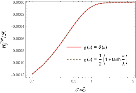
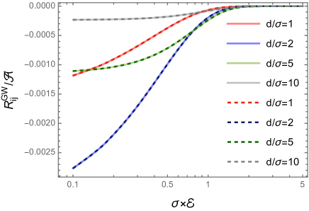
When :
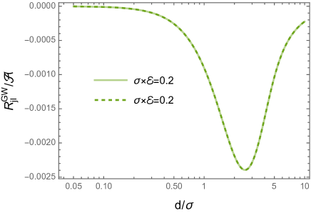
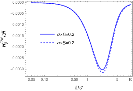
When we consider the expressions of from Eq. (V.2) and put the expression of and in it. The resulting integral can be carried out numerically and one can obtain the values of . In particular, in Fig. 2 we have plotted the in this scenario, as a function of the dimensionless detector energy gap . Whereas in Fig. 3 we have plotted as function of the mean of the switching time . From the left and right plots of Fig. 2 we notice that with increasing energy gap the decreases. Our observations suggest that with increasing distance between the detectors, first increases and then decreases. We also observe that with respect to , the is asymmetric, which suggests that for detectors switched on much earlier than there are negligible contributions due to the GW bursts with memory. At the same time, these memory bursts will have finite non-zero contribution if the detectors are switched on at some later time.
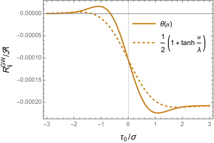
When :
When we consider the GW burst of the form of , we have . We use these expressions in Eq. (V.2) and obtain . In Figs. 2 and 3 we have plotted this component of the transition probability rate due to gravitational wave as functions of the dimensionless detector energy gap and mean of the switching time . The characteristics of these plots are similar to the ones for the scenario. Here also we observe that for detectors switched on much later than there will always be some contribution in the transition probability due to the GW burst.
When :
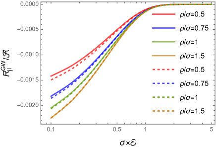
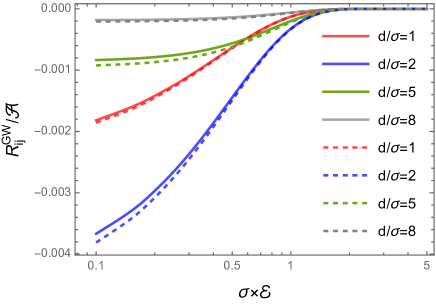
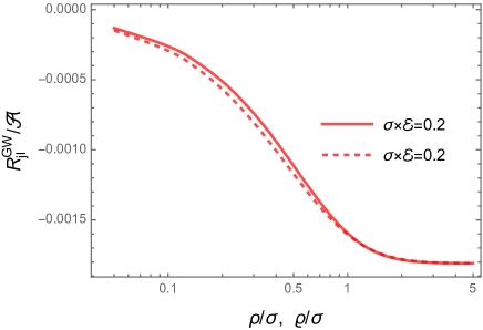
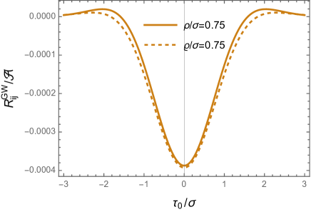
When we have , and we use these expressions in Eq. (V.2) to obtain . In Figs. 4 and 5 we have plotted due the present GW burst as functions of the dimensionless energy gap, duration of the GW, detector separation, and the mean of the switching time. Our observations show that with increasing switching time (or ) the contribution due to the GW increases and reaches a fixed maximum value. At the same time, with an increasing energy gap this contribution decreases. Whereas with increasing distance the first increases and then decreases, similar to the memory bursts. On the other hand, from Fig. 5 we observe that with respect to , the is symmetric around , i.e., around the origin of the GW burst, which is contrary to the memory burst scenario of Fig. 3.
When :
When we have , and we use these expressions in Eq. (V.2) and obtain . We have plotted this quantity for this specific burst profile in Figs. 4 and 5. The characteristics of these plots are similar to the ones obtained from the scenario. Here also we observe that is symmetric with respect to the mean time around . Therefore, for symmetric bursts at a much later time compared to there would not be any contribution due to the gravitational wave, which is in contrary to the memory GW burst profiles.
V.3 Total transition probability
Here we study the total transition probability corresponding to two entangled detectors moving on geodesic trajectories in GW burst backgrounds for finite interaction between the detectors and the field. Unlike the eternal switching scenario, the transition probabilities corresponding to finite Gaussian switching are finite. In particular, we consider the expression of from Eq. (V.2), which is of analytic form. Whereas, we get the expression of through the numerical integration of Eq. (V.2) corresponding to specific burst profiles. We would like to point out that for comoving detectors and in this limit . While taking this limit in Eq. (V.2) gives
| (53) |
which is the same expression as presented in Eq. (V.1), i.e., in this scenario corresponds to single detector response function . In the eternal switching scenario, we observed that only de-excitations, i.e., transitions from the Bell states ( and ) to the collective ground state () were possible. With the Gaussian switching we notice that transitions from the Bell states to the collective excited state () are also possible. These excitations are due to the transient switching and can lead to exciting outcomes, see Sriramkumar1996FinitetimeRO . Therefore, in this scenario, we focus our attention on these excitations. With the help of Eqs. (9) and (12) we express the transition probability rates, more specifically the relevant parts of it, from the symmetric or anti-symmetric Bell states to the collective excited state as
| (54a) | |||||
| (54b) | |||||
From the previous discussion and the discussion in Sec. V, we understood that and for . Then from Eq. 54 we can obtain the expressions
| (55a) | |||||
| (55b) | |||||
From the above expressions, one can notice that is free of any contribution from the GW. On the other hand, similar to the infinite switching scenario, here, for finite Gaussian switching carries the effect of the GW burst. It is to be noted that if one subtracts out the Minkowski from the above , then the resulting quantity depends entirely on the GW part. Furthermore, because of the symmetry , the difference will be exactly given by
| (56) |
where denotes the relevant quantity estimated in the gravitational wave background. In Sec. V, we observe that each from different GW burst backgrounds can have some signature reminiscent of the presence of GW memory. Thus one can notice that the quantity in Eq. (V.3) can be of help in isolating and identifying the GW memory as .
V.4 Inferences
From the above analysis, concerning finite Gaussian switching functions, we observe that excitations from the Bell states to the collective excited state are possible. Moreover, all the GW burst profiles with and without memory, contribute to the cross-transition probability. For GW bursts with memory if the detectors are switched on after the passing of the GW one will always get a non-zero finite contribution in the GW-induced cross-transition probability rate , see Fig. 3. At the same time, for bursts without memory, the contribution in the GW-induced cross-transition probability rate is maximum if the detectors are switched on during the passing of the GW, see Fig. 5. We believe these observations can provide us with important insight in regard to constructing experimental set-ups to identify GW memory. In particular one can identify the presence of memory after the passing of a GW burst by analysing the nature of the quantity , as elucidated in the previous subsection.
VI Discussion & concluding remarks
In this article, we have investigated the radiative process of two entangled Unruh-DeWitt detectors initially prepared in the maximally entangled Bell states. The detectors follow geodesic trajectories in a spacetime having linearized GW burst propagating over a flat background. We have considered different types of GW burst profiles, two asymmetric burst profiles in terms of the Heaviside theta and functions, and two symmetric profiles in terms of the Gaussian and -squared functions. As discussed previously, (also see Barman:2023aqk ) the symmetric profiles denote GW without memory and the asymmetric profiles signify GW bursts with memory. Furthermore, we have considered two types of switching, namely eternal switching of and finite Gaussian switching of , to investigate the features of the radiative process in the concerned background. The key observations from our investigation and their implications are as follows.
-
•
For eternal switching we find that the individual detector excitation in geodesic trajectories in a GW background vanishes, considering terms up to the first order in GW strength, i.e., taking terms . This phenomenon, evident from Eq. (31), is akin to the static detector scenario (see Barman:2023aqk ). Thus, it shows that the passage of a gravitational wave does not alter the particle content of a background, confirming the proposal in Gibbons:1975 . It is to be noted that even with finite Gaussian switching the individual detector transition probability does not contain any contribution from the GW (see Eq. (V.1)) and thus becomes identical with the one obtained in a Minkowski background (in this regard see Sriramkumar1996FinitetimeRO ). It should be mentioned that the particle creation for finite switching is attributed to the transient nature of the switching function, see Sriramkumar1996FinitetimeRO ; Barman:2022utm .
A tabular list of our observations Switching type GW profile: GW memory Features in the radiative process Eternal: Yes Non vanishing Yes Non vanishing No Vanishing No Vanishing Gaussian: Yes Non-zero in Yes Non-zero in No Non-zero peaked around No Non-zero peaked around Table 1: The above table lists our key observations regarding the radiative process of entangled Unruh-DeWitt detectors corresponding to different switching functions and GW burst profiles. -
•
In regard to entangled detectors, we observed that for eternal switching no excitation is possible, and only de-excitations are possible, see Eqs. (31-41). This observation implies that with eternal switching transitions from the Bell states to the collective excited state are not permitted, while transitions to the collective ground state are possible. On the other hand, with finite Gaussian switching, excitations, i.e., transitions to the collective excited state, are also possible, see Eqs. (V.1-V.2). This observation signifies that it is imperative to consider finite switching, if one measures only the collective excitation of an entangled system that follows geodesic trajectories to report the passage of GW.
-
•
In regard to entangled detectors and eternal switching we found that the GW-induced cross-transition probability rate is non-zero for the asymmetric profiles (profiles that correspond to GW memory) and it vanishes for the symmetric bursts (without GW memory). This fact is evident from the expressions of from Eqs. (37) and (38) corresponding to the asymmetric profiles and the expressions (40) and (41) concerning the symmetric GW profiles. Furthermore, as discussed in Sec. IV.3 due to GW effects the difference in the total transition probability rates between the symmetric and anti-symmetric Bell states will have a modified coefficient for the asymmetric bursts as compared to unity corresponding to the symmetric bursts. Thus, one could conclude that due to GW memory, there is a finite change in the total transition probability rates for eternal switching, which is absent for the bursts without memory. Moreover, the variation of with respect to the distance , which represents a function, will have a modified amplitude for GW profiles with memory.
-
•
Regarding entangled detectors and Gaussian switching we observed that the GW-induced cross-transition probabilities are non-zero for both the symmetric and asymmetric bursts. In particular, in all cases, the absolute value of this cross-transition probability rate decreases with increasing energy gap. It also increases with a small increase in separation between the detectors and then decreases as the separation is increased further. Moreover, for symmetric profiles, we observed that it is peaked around , i.e., when the Gaussian switching function peaks at the origin time of the GW. At the same time, for asymmetric bursts, it attains a saturated finite value after , and in the region it vanishes. Note that with GW memory in the region , is non-zero and finite. Thus, there will be a finite change in the transition probability for bursts with memory even after the GW burst has passed. This observation can form a basis for a future experimentally viable test of GW memory.
-
•
In Sec. V.3 we observed that by measuring a quantity that signifies the difference in between the GW and Minkowski backgrounds one can isolate the contribution of GW-induced cross-transition . In particular, this quantity is then given by . Then, in more simple terms, one can identify the effects of GW memory by measuring and noting in which profile this quantity saturates to a fixed non-zero value as one carries out this experiment placing detectors with multiple mean switching , i.e., by switching on the detectors at different times. In particular, in Table 1 we have listed all our key observations regarding the radiative process of entangled detectors in the presence of a GW burst for both eternal and finite Gaussian switching.
It has been known that the dynamics of entangled quantum probes can be affected by various system parameters such as the motion of the detectors, background curvature, thermal bath, spacetime dimensions, passing of gravitational wave, etc. In this regard, one can look into the introduction of the present manuscript for references. However, even if it depends on the passing of GW, whether it can also be affected by the memory in GW was not known previously. In this work, we considered a specific set-up comprising entangled quantum probes and discovered that it can identify GW memory backgrounds. For both eternal and Gaussian switching, we observed qualitative distinctions between the GW profiles with and without memory. The next immediate area to understand is how feasible these distinctions are in case one tries to measure it in an experimental set-up. In this regard, we believe an interesting and practical way forward could be through the utilization of quantum communication and key distribution, see Piveteau:2022gbr ; Bruschi:2013sua ; Bruschi:2014cma ; Barzel:2022tbf , where it is observed that quantum key distribution (QKD) protocols can efficiently capture the distortions in the photon wave packets caused due to the presence of curvature. Another practical way forward could be to understand the distortions in the atomic electron transitions in a hydrogen-like atom, see Chen:2023wpp , due to the presence of GW memory. These understandings can then be used to construct viable experimental set-up in identifying the GW memory. We are currently working in these directions and wish to present some of our findings in a future communication.
Acknowledgements.
We thank Sumanta Chakraborty for the initial idea for the project, and Bibhas Ranjan Majhi for comments on the manuscript. We would also like to thank Dawood Kothawala for the useful discussions and his comments on the manuscript. S.B. would like to thank the Science and Engineering Research Board (SERB), Government of India (GoI), for supporting this work through the National Post Doctoral Fellowship (N-PDF, File number: PDF/2022/000428). S.M. would like to acknowledge the Inspire Faculty Grant DST/INSPIRE/04/2022/001332, DST, Government of India, for financial support.Appendix A Consistency of the redefined Wightman function
Here, we elaborately explain the usage of the Wightman functions from Eqs. (27) and (29) provide the same total transition probability of Eq. (9). In this regard, let us consider the Wightman function from Eq. (27) to evaluate the transition coefficient from Eq. (10). This transition coefficient is
| (57) |
where . From this previous expression, one can easily find out the expression of by interchanging the positions of and . In particular, the expression of will be given by
| (58) |
In the total transition probability the quantities define individual transition probabilities. Thus they must be real and non-negative quantities. Whereas, from the expectation values of the monopole moment operators from Sec. II one can observe that for both the transitions from the symmetric or anti-symmetric Bell states to the ground state there will be in the total transition probability. Therefore the quantity must also be real. From Eqs. (A) and (A) one can evaluate this quantity to be
| (59) |
which clearly indicates that the imaginary contribution multiplied with should be zero. Our redefinition of the Wightman function in Eq. (29) does exactly that by selecting out the part of the Wightman function that gives real transition probability.
References
- (1) S. W. Hawking, “Particle creation by black holes,” Comm. Math. Phys. 43 no. 3, (1975) 199–220.
- (2) W. Unruh, “Notes on black hole evaporation,” Phys.Rev. D14 (1976) 870.
- (3) N. D. Birrell and P. C. W. Davies, Quantum fields in curved space. Cambridge Monographs on Mathematical Physics. Cambridge University Press, 1984.
- (4) D. N. Page, “Hawking radiation and black hole thermodynamics,” New J. Phys. 7 (2005) 203, arXiv:hep-th/0409024.
- (5) E. Martin-Martinez, I. Fuentes, and R. B. Mann, “Using Berry’s phase to detect the Unruh effect at lower accelerations,” Phys. Rev. Lett. 107 (2011) 131301, arXiv:1012.2208 [quant-ph].
- (6) M. Aspachs, G. Adesso, and I. Fuentes, “Optimal quantum estimation of the Unruh-Hawking effect,” Phys. Rev. Lett. 105 (2010) 151301, arXiv:1007.0389 [quant-ph].
- (7) D. Rideout et al., “Fundamental quantum optics experiments conceivable with satellites: Reaching relativistic distances and velocities,” Class. Quant. Grav. 29 (2012) 224011, arXiv:1206.4949 [quant-ph].
- (8) D. J. Stargen and K. Lochan, “Cavity Optimization for Unruh Effect at Small Accelerations,” Phys. Rev. Lett. 129 no. 11, (2022) 111303, arXiv:2107.00049 [gr-qc].
- (9) L. C. Crispino, A. Higuchi, and G. E. Matsas, “The Unruh effect and its applications,” Rev.Mod.Phys. 80 (2008) 787–838, arXiv:0710.5373 [gr-qc].
- (10) J. Rodriguez-Laguna, L. Tarruell, M. Lewenstein, and A. Celi, “Synthetic Unruh effect in cold atoms,” Phys. Rev. A 95 no. 1, (2017) 013627, arXiv:1606.09505 [cond-mat.quant-gas].
- (11) M. P. Blencowe and H. Wang, “Analogue Gravity on a Superconducting Chip,” Phil. Trans. Roy. Soc. Lond. A 378 no. 2177, (2020) 20190224, arXiv:2003.00382 [quant-ph].
- (12) C. Gooding, S. Biermann, S. Erne, J. Louko, W. G. Unruh, J. Schmiedmayer, and S. Weinfurtner, “Interferometric Unruh detectors for Bose-Einstein condensates,” Phys. Rev. Lett. 125 no. 21, (2020) 213603, arXiv:2007.07160 [gr-qc].
- (13) S. Biermann, S. Erne, C. Gooding, J. Louko, J. Schmiedmayer, W. G. Unruh, and S. Weinfurtner, “Unruh and analogue Unruh temperatures for circular motion in 3+1 and 2+1 dimensions,” Phys. Rev. D 102 no. 8, (2020) 085006, arXiv:2007.09523 [gr-qc].
- (14) S. Onoe, T. L. M. Guedes, A. S. Moskalenko, A. Leitenstorfer, G. Burkard, and T. C. Ralph, “Realizing a rapidly switched Unruh-DeWitt detector through electro-optic sampling of the electromagnetic vacuum,” Phys. Rev. D 105 no. 5, (2022) 056023, arXiv:2103.14360 [quant-ph].
- (15) J. Hu, L. Feng, Z. Zhang, and C. Chin, “Quantum simulation of Unruh radiation,” Nature Phys. 15 no. 8, (2019) 785–789, arXiv:1807.07504 [physics.atom-ph].
- (16) B. Reznik, “Entanglement from the vacuum,” Found. Phys. 33 (2003) 167–176, arXiv:quant-ph/0212044.
- (17) F. Benatti and R. Floreanini, “Entanglement generation in uniformly accelerating atoms: Reexamination of the unruh effect,” Phys. Rev. A 70 (Jul, 2004) 012112.
- (18) I. Fuentes-Schuller and R. B. Mann, “Alice falls into a black hole: Entanglement in non-inertial frames,” Phys. Rev. Lett. 95 (2005) 120404, arXiv:quant-ph/0410172.
- (19) J. L. Ball, I. Fuentes-Schuller, and F. P. Schuller, “Entanglement in an expanding spacetime,” Phys. Lett. A 359 (2006) 550–554, arXiv:quant-ph/0506113.
- (20) M. Cliche and A. Kempf, “The relativistic quantum channel of communication through field quanta,” Phys. Rev. A 81 (2010) 012330, arXiv:0908.3144 [quant-ph].
- (21) S.-Y. Lin and B. Hu, “Entanglement creation between two causally disconnected objects,” Phys. Rev. D 81 (2010) 045019, arXiv:0910.5858 [quant-ph].
- (22) E. Martin-Martinez and N. C. Menicucci, “Cosmological quantum entanglement,” Class. Quant. Grav. 29 (2012) 224003, arXiv:1204.4918 [gr-qc].
- (23) G. Salton, R. B. Mann, and N. C. Menicucci, “Acceleration-assisted entanglement harvesting and rangefinding,” New J. Phys. 17 no. 3, (2015) 035001, arXiv:1408.1395 [quant-ph].
- (24) E. Martin-Martinez, A. R. H. Smith, and D. R. Terno, “Spacetime structure and vacuum entanglement,” Phys. Rev. D 93 no. 4, (2016) 044001, arXiv:1507.02688 [quant-ph].
- (25) W. Zhou and H. Yu, “Resonance interatomic energy in a Schwarzschild spacetime,” Phys. Rev. D 96 no. 4, (2017) 045018.
- (26) H. Cai and Z. Ren, “Transition processes of a static multilevel atom in the cosmic string spacetime with a conducting plane boundary,” Sci. Rep. 8 no. 1, (2018) 11802.
- (27) Y. Pan and B. Zhang, “Influence of acceleration on multibody entangled quantum states,” Phys. Rev. A 101 no. 6, (2020) 062111, arXiv:2009.05179 [quant-ph].
- (28) S. Barman and B. R. Majhi, “Radiative process of two entangled uniformly accelerated atoms in a thermal bath: a possible case of anti-Unruh event,” JHEP 03 (2021) 245, arXiv:2101.08186 [gr-qc].
- (29) H. K, S. Barman, and D. Kothawala, “Universal role of curvature in vacuum entanglement,” Phys. Rev. D 109 no. 6, (2024) 065017, arXiv:2311.15019 [gr-qc].
- (30) J.-T. Hsiang, H.-T. Cho, and B.-L. Hu, “Graviton physics: Quantum field theory of gravitons, graviton noise and gravitational decoherence – a concise tutorial,” arXiv:2405.11790 [hep-th].
- (31) J.-I. Koga, G. Kimura, and K. Maeda, “Quantum teleportation in vacuum using only Unruh-DeWitt detectors,” Phys. Rev. A 97 no. 6, (2018) 062338, arXiv:1804.01183 [gr-qc].
- (32) J.-i. Koga, K. Maeda, and G. Kimura, “Entanglement extracted from vacuum into accelerated Unruh-DeWitt detectors and energy conservation,” Phys. Rev. D 100 no. 6, (2019) 065013, arXiv:1906.02843 [quant-ph].
- (33) J. Zhang and H. Yu, “Entanglement harvesting for Unruh-DeWitt detectors in circular motion,” Phys. Rev. D 102 no. 6, (2020) 065013, arXiv:2008.07980 [quant-ph].
- (34) D. Barman, S. Barman, and B. R. Majhi, “Entanglement harvesting between two inertial Unruh-DeWitt detectors from nonvacuum quantum fluctuations,” Phys. Rev. D 106 no. 4, (2022) 045005, arXiv:2205.08505 [gr-qc].
- (35) M. Cliche and A. Kempf, “Vacuum entanglement enhancement by a weak gravitational field,” Phys. Rev. D 83 (2011) 045019, arXiv:1008.4926 [quant-ph].
- (36) S. Kukita and Y. Nambu, “Harvesting large scale entanglement in de Sitter space with multiple detectors,” Entropy 19 no. 9, (2017) 449, arXiv:1708.01359 [gr-qc].
- (37) S. Barman, D. Barman, and B. R. Majhi, “Entanglement harvesting from conformal vacuums between two Unruh-DeWitt detectors moving along null paths,” JHEP 09 (2022) 106, arXiv:2112.01308 [gr-qc].
- (38) S. Barman and B. R. Majhi, “Optimization of entanglement harvesting depends on the extremality and nonextremality of a black hole,” arXiv:2301.06764 [gr-qc].
- (39) Q. Xu, S. A. Ahmad, and A. R. H. Smith, “Gravitational waves affect vacuum entanglement,” Phys. Rev. D 102 no. 6, (2020) 065019, arXiv:2006.11301 [quant-ph].
- (40) F. Gray, D. Kubiznak, T. May, S. Timmerman, and E. Tjoa, “Quantum imprints of gravitational shockwaves,” JHEP 11 (2021) 054, arXiv:2105.09337 [hep-th].
- (41) E. G. Brown, “Thermal amplification of field-correlation harvesting,” Phys. Rev. A 88 no. 6, (2013) 062336, arXiv:1309.1425 [quant-ph].
- (42) P. Simidzija and E. Martín-Martínez, “Harvesting correlations from thermal and squeezed coherent states,” Phys. Rev. D 98 no. 8, (2018) 085007, arXiv:1809.05547 [quant-ph].
- (43) D. Barman, S. Barman, and B. R. Majhi, “Role of thermal field in entanglement harvesting between two accelerated Unruh-DeWitt detectors,” JHEP 07 (2021) 124, arXiv:2104.11269 [gr-qc].
- (44) R. H. Dicke, “Coherence in spontaneous radiation processes,” Phys. Rev. 93 (Jan, 1954) 99–110.
- (45) E. Arias, J. Dueñas, G. Menezes, and N. Svaiter, “Boundary effects on radiative processes of two entangled atoms,” JHEP 07 (2016) 147, arXiv:1510.00047 [quant-ph].
- (46) Z. Ficek and R. Tanaś, “Entangled states and collective nonclassical effects in two-atom systems,” Physics Reports 372 no. 5, (2002) 369–443.
- (47) G. Picanço, N. F. Svaiter, and C. A. D. Zarro, “Radiative Processes of Entangled Detectors in Rotating Frames,” JHEP 08 (2020) 025, arXiv:2002.06085 [hep-th].
- (48) S. Barman, B. R. Majhi, and L. Sriramkumar, “Radiative processes of single and entangled detectors on circular trajectories in dimensional Minkowski spacetime,” arXiv:2205.01305 [gr-qc].
- (49) G. Menezes, “Entanglement dynamics in a Kerr spacetime,” Phys. Rev. D 97 no. 8, (2018) 085021, arXiv:arXiv:1712.07151 [gr-qc].
- (50) H. Cai and Z. Ren, “Radiative processes of two entangled atoms in cosmic string spacetime,” Class. Quant. Grav. 35 no. 2, (2018) 025016.
- (51) X. Liu, Z. Tian, J. Wang, and J. Jing, “Radiative process of two entanglement atoms in de Sitter spacetime,” Phys. Rev. D 97 no. 10, (2018) 105030, arXiv:1805.04470 [gr-qc].
- (52) D.-W. Chiou, “Response of the Unruh-DeWitt detector in flat spacetime with a compact dimension,” arXiv:1605.06656 [gr-qc].
- (53) S. Barman, I. Chakraborty, and S. Mukherjee, “Entanglement harvesting for different gravitational wave burst profiles with and without memory,” JHEP 09 (2023) 180, arXiv:2305.17735 [gr-qc].
- (54) S.-M. Wu, R.-D. Wang, X.-L. Huang, and Z. Wang, “Does gravitational wave assist vacuum steering and Bell nonlocality?,” arXiv:2405.07235 [gr-qc].
- (55) M. Favata, “The gravitational-wave memory effect,” Class. Quant. Grav. 27 (2010) 084036, arXiv:1003.3486 [gr-qc].
- (56) I. Chakraborty and S. Kar, “A simple analytic example of the gravitational wave memory effect,” Eur. Phys. J. Plus 137 no. 4, (2022) 418, arXiv:2202.10661 [gr-qc].
- (57) I. Chakraborty, “Kundt wave geometries in Eddington-inspired Born-Infeld gravity: New solutions and memory effects,” Phys. Rev. D 105 no. 2, (2022) 024063, arXiv:2110.02295 [gr-qc].
- (58) A. Tolish and R. M. Wald, “Retarded Fields of Null Particles and the Memory Effect,” Phys. Rev. D 89 no. 6, (2014) 064008, arXiv:1401.5831 [gr-qc].
- (59) M. Maggiore, Gravitational Waves: Volume 1: Theory and Experiments. OUP Oxford, 2007.
- (60) S. J. Kovacs and K. S. Thorne, “The Generation of Gravitational Waves. 4. Bremsstrahlung,” Astrophys. J. 224 (1978) 62–85.
- (61) J. Garcia-Bellido and S. Nesseris, “Gravitational wave bursts from Primordial Black Hole hyperbolic encounters,” Phys. Dark Univ. 18 (2017) 123–126, arXiv:1706.02111 [astro-ph.CO].
- (62) A. Hait, S. Mohanty, and S. Prakash, “Frequency space derivation of linear and non-linear memory gravitational wave signals from eccentric binary orbits,” arXiv:2211.13120 [gr-qc].
- (63) M. Mukhopadhyay, C. Cardona, and C. Lunardini, “The neutrino gravitational memory from a core collapse supernova: phenomenology and physics potential,” JCAP 07 (2021) 055, arXiv:2105.05862 [astro-ph.HE].
- (64) N. Sago, K. Ioka, T. Nakamura, and R. Yamazaki, “Gravitational wave memory of gamma-ray burst jets,” Phys. Rev. D 70 (2004) 104012, arXiv:gr-qc/0405067.
- (65) C. Rodríguez-Camargo, N. Svaiter, and G. Menezes, “Finite-time response function of uniformly accelerated entangled atoms,” Annals Phys. 396 (2018) 266–291, arXiv:1608.03365 [quant-ph].
- (66) G. Picanço, N. F. Svaiter, and C. A. Zarro, “Radiative Processes of Entangled Detectors in Rotating Frames,” JHEP 08 (2020) 025, arXiv:2002.06085 [hep-th].
- (67) J. Garriga and E. Verdaguer, “Scattering of quantum particles by gravitational plane waves,” Phys. Rev. D 43 (Jan, 1991) 391–401.
- (68) L. Sriramkumar and T. Padmanabhan, “Finite-time response of inertial and uniformly accelerated Unruh - DeWitt detectors,” Class. Quant. Grav. 13 (1996) 2061–2079, arXiv:gr-qc/9408037.
- (69) G. Gibbons, “Quantized fields propagating in plane-wave spacetimes,” Commun. Math. Phys. 45 (1975) 191–202.
- (70) A. Piveteau, J. Pauwels, E. Hrakansson, S. Muhammad, M. Bourennane, and A. Tavakoli, “Entanglement-assisted quantum communication with simple measurements,” Nature Commun. 13 no. 1, (2022) 7878, arXiv:2205.09602 [quant-ph].
- (71) D. E. Bruschi, T. Ralph, I. Fuentes, T. Jennewein, and M. Razavi, “Spacetime effects on satellite-based quantum communications,” Phys. Rev. D 90 (2014) 045041, arXiv:1309.3088 [quant-ph].
- (72) D. E. Bruschi, A. Datta, R. Ursin, T. C. Ralph, and I. Fuentes, “Quantum estimation of the Schwarzschild spacetime parameters of the Earth,” Phys. Rev. D 90 no. 12, (2014) 124001, arXiv:1409.0234 [quant-ph].
- (73) R. Barzel, D. E. Bruschi, A. W. Schell, and C. Laemmerzahl, “Observer dependence of photon bunching: The influence of the relativistic redshift on Hong-Ou-Mandel interference,” Phys. Rev. D 105 no. 10, (2022) 105016, arXiv:2202.07950 [gr-qc].
- (74) B.-H. Chen and D.-W. Chiou, “Atomic electron transitions of hydrogen-like atoms induced by gravitational waves,” arXiv:2312.12802 [gr-qc].