Synchronization on circles and spheres
with nonlinear interactions
Abstract
We consider the dynamics of points on a sphere in () which attract each other according to a function of their inner products. When is linear (), the points converge to a common value (i.e., synchronize) in various connectivity scenarios: this is part of classical work on Kuramoto oscillator networks. When is exponential (), these dynamics correspond to a limit of how idealized transformers process data, as described by Geshkovski et al. (2024). Accordingly, they ask whether synchronization occurs for exponential .
In the context of consensus for multi-agent control, Markdahl et al. (2018) show that for (spheres), if the interaction graph is connected and is increasing and convex, then the system synchronizes. What is the situation on circles ()? First, we show that being increasing and convex is no longer sufficient. Then we identify a new condition (that the Taylor coefficients of are decreasing) under which we do have synchronization on the circle. In so doing, we provide some answers to the open problems posed by Geshkovski et al. (2024).
1 Introduction
Motivated by open questions Geshkovski et al. (2024) raised in their paper “A mathematical perspective on transformers,” (specifically, Problems 4 and 5) we consider gradient flow to maximize111In contrast, running negative gradient flow may or may not take us to a minimum of . That problem is also interesting (and quite different) as it leads to configurations of points that are well spread out on the sphere. This is related to Thomson’s problem and Smale’s 7th problem with . the following function defined for points on the unit sphere in :
| (P) |
The real numbers are the weights of a graph () and the function is twice continuously differentiable. We assume is strictly increasing, so that the global maxima correspond to synchronized states: . The question is: under what conditions does gradient flow reliably converge to such a state?
This is well studied in the linear case () as it is equivalent to synchronization of Kuramoto networks of phases (Kuramoto, 1975) and (by extension) on spheres. Synchronization questions also go by the name “consensus” in the context of multi-agent control (Sarlette and Sepulchre, 2009a). From that literature (see Section 2), we expect markedly different behavior between synchronization on circles () and spheres (). The graph structure matters greatly on circles whereas, for higher-dimensional spheres, gradient flow converges to a synchronized state from almost every initial configuration, as long as the graph is connected. The key difference between the two cases is that spheres are simply connected but circles are not (Markdahl, 2021). The results in this paper also reflect this dichotomy.
In the paper of Geshkovski et al. (2024, Problems 4 and 5), problem (P) arises for complete graph with unit weights ( for all ) and nonlinear set to be
| (1) |
where is an “inverse temperature” in the language of statistical physics. The limit corresponds to the linear case .
That setting materializes through their study of an idealized model of how input data (tokens) are processed in infinitely deep neural networks with an architecture inspired by transformers. In that context, the interacting particles on the sphere correspond to tokens, and time for the gradient flow corresponds to depth in the network.222Geshkovski et al. (2024) obtain gradient flow on with by modeling deep networks composed of self-attention and layer-normalization layers. In the self-attention layers, replacing the exponential of the softmax with gives, in exactly the same way, the gradient flow on with general (the object of our study). This step of modelling discrete layers as continuous time variables is in line with previous literature on modeling residual neural networks as neural ODEs (Chen et al., 2018; E, 2017; Haber and Ruthotto, 2017). Neural ODEs to study transformers were first proposed in (Lu et al., 2020; Dutta et al., 2021; Sander et al., 2022).
For random initial configurations, Geshkovski et al. (2024) observed in their setting that the points always converge to a global maximum of , namely, . This is sensible since is maximal when , but it is not a foregone conclusion given that spheres are nonconvex.
Appendix G includes Matlab code for readers who wish to explore the landscape of (P) and the associated dynamical system with various choices of parameters. It requires the Manopt toolbox (Boumal et al., 2014), which is under GNU GPLv3 license.
Via landscapes
To analyze the typical asymptotic behavior of this dynamical system, it is sufficient to understand the structure of some critical points of , rather than tracking the entire dynamics. Indeed, if (hence ) is real-analytic, then gradient flow converges to a critical point (Łojasiewicz, 1965). Assuming a uniformly random initialization,333Or any other absolutely continuous probability measure. the Hessian at that critical point is almost surely negative semidefinite owing to the center-stable manifold theorem (Shub, 1987, Thm. III.7, Ex. III.3). (Though classical, this argument is rarely spelled out: see (Geshkovski et al., 2024, App. B) for welcome details.)
Thus, to confirm that gradient flow almost surely converges to a synchronized state, it is sufficient to show that points where the gradient of is zero and the Hessian is negative semidefinite are in fact synchronized (in particular, that they are global maxima). The gradient and Hessian are defined with respect to the usual Riemannian metric on the sphere: see Appendix A for explicit formulas.
Positive answers, obstructions and remaining open questions
To set the scene, we first state the following theorem to handle . In particular, it positively answers the questions of Geshkovski et al. (2024) for (see Corollary 2). This follows directly from (Markdahl et al., 2018, Thm. 13). We give a short proof in Appendix C based on a randomized selection of tangent vectors plugged into the Hessian quadratic form, paralleling the proof in (McRae and Boumal, 2024, §4) for synchronization of rotations.
Theorem 1 (Spheres, Markdahl et al. (2018, Thm. 13)).
Fix . Assume
-
1.
the ambient dimension satisfies ,
-
2.
the undirected graph defined by the weights is connected, and
-
3.
and for all .
Then, critical points of where the Hessian is negative semidefinite are global maxima of . In particular: local maxima are global maxima, they are the synchronized states (), and (if is real-analytic) gradient flow converges to a synchronized state from almost every initialization.
Corollary 2.
Theorem 1 applies for and for with all .
Let us go through the assumptions in Theorem 1. If is not positive ( not monotonously increasing) there may be global maxima that are not synchronized: see analyzed in Appendix F. If is not nonnegative ( not convex) there may be non-global local maxima: consider a tetrahedron () with . If the graph is not connected, then the claims of Theorem 1 still apply to each connected component separately.
The assumption is more interesting—and indeed necessary. As mentioned above, in the linear case () there are counterexamples when . However, these are for incomplete graphs (the simplest example is a cycle graph; see, e.g., Townsend et al. (2020) for many more). In contrast, the setting in (Geshkovski et al., 2024) centers on complete graphs.
Remarkably, with nonlinear and , even a complete graph with unit weights can harbor spurious local maxima. In Section 5, we construct a single function which satisfies the assumptions of Theorem 1 yet for which, with , the conclusion of that theorem fails for all .
Theorem 3 (Circles).
Let , and consider the complete graph with for all . For and , define
which is real-analytic and satisfies for all . There exist and such that, for all , gradient flow on (P) with and uniformly random initialization converges to a spurious local maximum (not synchronized) with positive probability.
Intuitively, Theorem 3 relies on the fact that there are functions and configurations such that (P) locally behaves much like an incomplete graph with linear (in particular, a circulant graph in a “twisted state” configuration, which is a well-known source of spurious local maxima in the linear case; see, e.g., Wiley et al. (2006); Townsend et al. (2020)).
Still, Theorem 3 does not exclude the possibility that the landscape is benign for when .444As an example, for fixed , Sarlette and Sepulchre (2009b, §6) construct a such that the particles synchronize as long as the graph is connected, but it is different from and it does not work for all . We show that this is indeed true for in Section 4. This follows as a corollary of our next theorem, which requires the Taylor expansion coefficients of to be nonincreasing. That corollary improves on (Geshkovski et al., 2024, Thm. 5.3) which requires .
Theorem 4.
Fix . Assume and for all , and also that
| for all | with |
Let the weights of the graph satisfy for some with positive entries (in particular, the graph is complete). Then all the same conclusions as in Theorem 1 apply. The assumption can be relaxed to if for all .
Corollary 5 (Small ).
Theorem 4 applies for and for with . It also applies for for all (Thomson’s problem corresponds to ).
Geshkovski et al. (2024) also argue that synchronization occurs almost surely for . We repeat their argument in Appendix E with minor changes to handle an arbitrary connected graph and more general , and to make all quantities explicit.
Theorem 6.
Corollary 7 (large , Geshkovski et al. (2024, Thm. 5.3)).
Fix and . Let with , and consider a connected graph with weights . Then all the same conclusions as in Theorem 1 apply.
It remains open whether the same holds for values of between 1 and when .
Finally, we use a different proof in Appendix F to show that the landscape is benign in the quadratic case (), although the global maxima are synchronized only up to sign.
Remark 8.
To model transformers, Geshkovski et al. (2024) consider two dynamical systems: SA (for self-attention) and USA. Problem (P) corresponds to USA. In their §3.4 and Remark C.1, they note that the two models correspond to gradient flow on the same energy (namely, with ) only with two different Riemannian metrics on the product of spheres. As the Riemannian metric has no effect on the limit points of gradient flow, our landscape analyses apply directly to both models.
2 Related work
Problem (P) is closely connected to the Kuramoto model for a network of coupled oscillators (Kuramoto, 1975; Acebrón et al., 2005), which has deep roots in the dynamical systems literature. The “homogeneous” variant considers the following dynamics for time-varying angles :
| (3) |
This is precisely the gradient flow of (P) in the linear case () with under the change of variable . A basic question is which graphs have the property that the system converges to the synchronized state from almost every initial configuration. The literature is vast: see the references below and the survey by Dörfler and Bullo (2014) (particularly §5). For our purposes, the key results are the following.
For complete graphs and, more generally, sufficiently dense or expander-like graphs, the dynamical system (3) synchronizes from almost every initialization (Sepulchre et al., 2007; Taylor, 2012; Kassabov et al., 2021; Abdalla et al., 2022). In contrast, for sparse or structured connected graphs, the dynamics (3) have stable equilibria other than the synchronized state (equivalently, (P) with and linear has spurious local maxima). A rich source of such spurious configurations consists of “twisted states” on a circulant or otherwise ring-like graph (Wiley et al., 2006; Canale and Monzón, 2015; Townsend et al., 2020; Yoneda et al., 2021). One can also construct more exotic counterexamples, including graphs with manifolds of stable equilibria of arbitrary dimension (Sclosa, 2023).
In higher dimensions (), less attention has been given to this problem. Relevant works for synchronization on spheres include (Olfati-Saber, 2006; Li and Spong, 2014; Caponigro et al., 2015; Lageman and Sun, 2016), though none of these guarantee synchronization almost surely. The key work for us is by Markdahl et al. (2018), who show that a broad class of consensus algorithms on the sphere succeed as long as the interaction graph is connected. Hence, synchronization/consensus on spheres is fundamentally simpler than on circles. One may also entertain synchronization on more general manifolds (Sarlette and Sepulchre, 2009a; Markdahl, 2021). The rotation groups are of particular interest in applications (and they constitute another way to generalize circles).
If we minimize rather than maximize , we obtain a packing problem. These have been extensively studied in the literature (e.g., Cohn and Kumar (2007)). Packing on the circle or sphere is closely related to Smale’s 7th problem and Thomson’s problem, which ask for the minimal energy configurations of charges constrained to lie on a circle or sphere. Among this line of work, most relevant to us is the work of Cohn (1960), who considers Thomson’s problem on the circle. Using Morse theory, Cohn (1960) completely characterizes the minima and critical points of , and their signatures, when and (and for other similar ). It is unclear to us how to apply the techniques of Cohn (1960) to the present setting: crucially with , the Hessian of on the circle corresponds to a Laplacian with all nonpositive weights. This is a substantial departure from our setting: see the open questions in Section 6.
3 Riemannian geometry tools and optimality conditions
Endow with the inner product . The unit sphere is a Riemannian submanifold of : the tangent space inherits the Euclidean inner product as a subspace of . Formally, in (P) is defined on the product manifold
with the product Riemannian structure. In this matrix notation, the points are arranged as the columns of , extracts the diagonal of a matrix, and is the all-ones vector (sometimes denoted if we want to emphasize the dimension). The cost function is
where is the Frobenius inner product, and applies entrywise (). The symmetric matrix holds the graph weights .
Based on these choices, we can derive expressions for the Riemannian gradient and Hessian of , and deduce necessary optimality conditions for (P). These are standard computations: see Appendix A.
Since our results in Theorems 3 and 4 only require proofs for , we only spell out the conditions for that case here. This is simpler in part because the tangent space of a circle is one-dimensional, so that the Riemannian Hessian can be expressed as an ordinary matrix.
The Riemannian Hessian for exhibits a Laplacian structure, defined as follows. Given a symmetric matrix , the Laplacian of the associated graph (where we think of as the weight between nodes and ) is
| (4) |
where forms a diagonal matrix. As a quadratic form, it is well known that . In particular, if the weights are nonnegative, then . If, furthermore, the graph is connected, then .
We now characterize second-order critical points. In the following, sets all off-diagonal entries of a matrix to zero, denotes the entrywise (Hadamard) matrix product, and denotes entrywise squaring.
Lemma 9.
Let . Assume is twice continuously differentiable. The eigenvalues of the Hessian of at are equal to the eigenvalues of , where is the Laplacian (4) for the graph with weights
| where | (5) |
The Riemannian gradient at is zero (i.e., is critical) and the Riemannian Hessian at is negative semidefinite if and only if
| (6) | ||||
| (7) |
4 A sufficient condition for synchronization on the circle: Theorem 4
Given with positive entries, define the complete graph . (The notation echoes classical work where each is a particle with charge and is their associated potential (Cohn, 1960).) From Theorem 1, we know that in dimension it is sufficient for to be a strictly increasing convex function to rule out spurious local maxima for . From Theorem 3, we also know that this is not sufficient when . Yet, experimentally, even with we do not know of spurious maximizers when (1). Thus, it appears that has additional favorable properties.
In this section, we show as much for up to 1. Specifically, we prove Theorem 4. Our argument relies crucially on the Schur product theorem (Horn and Johnson, 1991, Thm. 5.2.1).
To prove Theorem 1 for spheres (see Appendix C), we chose a random direction , and then moved all points in that same direction using . This approach works for spheres, but falls short when applied to circles. It is natural to try to choose the common direction more purposefully. Albeit indirectly, the proof below moves all the points in the direction of their weighted mean . See Remark 11 at the end of this section.
We start with a lemma showing that we are done if we can show lie in a common (closed) hemisphere (we also use this in the proof of Theorem 6). This strengthens existing results for an open hemisphere by Markdahl et al. (2018, Prop. 12) and, in their setting, Geshkovski et al. (2024, Lem. 4.2). The rank-deficient case (which is treated separately in the proof) resembles familiar results for Burer–Monteiro relaxations (see, for example, Journée et al. (2010, Thm. 7)), but the standard arguments used in that literature do not directly apply because we are maximizing a convex function (and not minimizing).
Lemma 10.
Assume for all and that the graph with weights is connected. Let be a critical point of where the Hessian is negative semidefinite. If there exists a nonzero such that (entrywise; that is, the points lie in a common closed hemisphere), then is a global maximum. Such a vector exists if .
See Appendix B for a proof. With this, we can prove the main result of this section.
Proof of Theorem 4.
Fix (the case holds by Theorem 1). Lemma 9 provides
| and |
where is the Laplacian (4) of the graph with weights and (7). Since , it follows that and so .
Multiply the matrix inequality left and right by and to compress it to a matrix inequality. Crucially, this allows us to use the first-order condition:
| (8) |
By the assumption on , it holds that
for all , with for all . In particular,
Plugging this back into (8) yields
The Schur product theorem states that . Using and the assumption that plus the assumption that etc., we deduce
Since , we also have . With , the above can be restated as:
| (9) |
The matrix on the left-hand side has rank 1. The matrix in the middle is positive semidefinite since and .
If , then the matrix in the middle of inequality (9) must have rank equal to , using for all . The result then follows, because inequality (9) therefore implies , and Lemma 10 handles .
For , we assume and take a closer look at . Since and , it follows that if and only if . We consider two cases.
First, suppose . This means the graph of is disconnected. For in different connected components, , so . Since has at least two nonempty connected components, this implies for all (simply observe that each is in a component that is different from that of or ). Thus, and the result again follows from Lemma 10.
Remark 11.
The proof above moves all points in the direction of their weighted mean . To see this, note that all cases at the end of the proof are handled (explicitly or implicitly) by hitting (9) with an appropriately chosen vector proportional to , where . One can verify (see the proof of Lemma 9 in Appendix A) that this translates to tangent vectors .
5 Obstacles to synchronization on the circle: Theorem 3
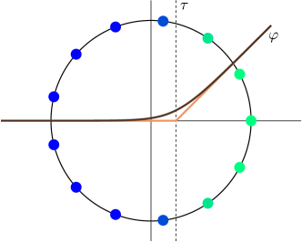
The circle () stands out among “spheres” in that it is not simply connected: the circle itself (a closed loop) cannot be continuously collapsed into a single point while staying on the circle, whereas, say, the equator can be collapsed to a single point on a sphere. Accordingly, to construct non-synchronizing scenarios on the circle, it makes sense to entertain configurations of points that “go around” the circle. The simplest such configuration is when all points lie on a regular -gon as follows (see Figure 1):
| with | for | (10) |
In this section we prove Theorem 3: when there exists a real-analytic with such that has a spurious local maximum for all . Let us sketch the proof. As a first step, we show that for each there is a such that the regular -gon is a spurious local maximum of with (Lemma 13 below); this follows from a well-known result for linear synchronization on the circle (Lemma 12). In order to build a single which works for all as in Theorem 3, we then fix some integer (e.g., ) and distribute points on the regular -gon with roughly points at each vertex. This configuration may not be critical for with (e.g., if is not a multiple of ), but we argue that it is close to a spurious critical point (and hence that one exists) provided is large enough (combine Lemmas 14 and 15 below). Finally, we exhibit a that covers all . Now let us proceed to the full proof.
For the linear synchronization problem on the circle (), it is well known that the regular -gon configuration (10) (with large enough ) is a spurious local maximum when the weight matrix corresponds to a (circulant) nearest-neighbor graph in which every node is connected to at most of its nearest neighbors. This observation is due to Wiley et al. (2006).
In our setting, we can see this as taking the complete graph and the ReLU-type function
| (11) |
with at least : see Figure 1. This is valid for large . To handle all , we reduce connectivity and require . We also require to ensure that each point interacts with at least its two nearest neighbors. The following lemma can be checked with formulas by Ling et al. (2019, §5.3), who obtain the eigenvalues of the Hessian at the regular -gon in closed form using a Fourier transform.
Lemma 12.
[Wiley et al. (2006), Ling et al. (2019, §5.3)] Given , let lie on a regular -gon (10). Fix such that .555This condition ensures that none of the inner products for the -gon lie on the kink of the ReLU. With as in (11) and , the point is critical for , and is negative666Throughout Section 5, “negative definite Hessian” means all eigenvalues of the Hessian are negative except for the single zero eigenvalue which appears due to the global rotation symmetry of the problem. definite.
The next step is simple: we smooth the ReLU (11) and, by continuity, the regular -gon remains a spurious local maximum. In order to ensure is real-analytic, we apply the log-sum-exp smoothing
| (12) |
with parameter .
Lemma 13.
Proof of Lemma 13.
From Lemma 9, one can easily verify by symmetry that the regular -gon is critical for for any such that is differentiable in a neighborhood of . We now study , which is well defined (even at ) since we assume for . Lemma 12 gives that is negative6 definite. Hence, it is enough to show that the curve is continuous from the right at . We can then conclude using the continuity of eigenvalues. (More formally, one should remove the trivial zero eigenvalue of the Hessian by fixing one of the points, or passing to the quotient, and then applying this argument.) The function only appears in through and (see Lemma 16 in Appendix A). Therefore, it is enough to show that for any fixed , both
| and |
are continuous from the right at . This is readily apparent from their expressions. ∎
Lemma 13 does not give a which works for all as in Theorem 3 because, as grows, it seems that must decrease to zero. However, we can circumvent this issue by the following observation. Fix and let be an integer multiple of . Consider the configuration of points on the circle where points are placed at the vertices of a regular -gon—we call this configuration the “repeated -gon.” As the -gon is a spurious local maximum for on points with , it stands to reason that the repeated -gon should be a spurious local maximum on points with (when is a multiple of ). This is indeed true. We give a proof of the following (more general) statement in Appendix D. (Allowing arbitrary , as opposed to just a multiple of , shall be useful for handling the cases where is not a multiple of .)
Lemma 14.
For fixed , this shows that has a spurious local maximum with for points, where is a multiple of (and is chosen as in Lemma 12 with replaced by ). To handle a number of points that is not a multiple of (i.e., ), first place points on each vertex of the regular -gon, then distribute the extraneous points arbitrarily on the vertices. This configuration is unlikely to be a critical point; however, it is close to one: if the total number of points is sufficiently large, the few extra points should only cause a minor perturbation from what was a (strict) spurious local maximum.
In Lemma 15, this intuition is made rigorous via the implicit function theorem. In the language of Lemma 14, we let be the regular -gon, and we take each to be an integer close to ; consequently is close to . We rescale by so that itself becomes close (this scaling does not affect the landscape of ). The proof is in Appendix D.
Lemma 15.
Fix odd. There exists such that if and satisfy
| and |
then has a spurious critical point with negative6 definite Hessian.
Proof of Theorem 3.
Fix . Write with remainder . Let . Note that if is sufficiently large then is arbitrarily close to . Invoke Lemma 15 to select . Set such that for all . If
| and | (14) |
then has a spurious critical point with negative6 definite Hessian: call it .
6 Conclusions and perspectives
We conclude with a list of open questions for , and (complete graph).
-
•
(All ) Do we have synchronization for ?
- •
-
•
(Critical configurations) We say a configuration consists of clusters if there exist such that , i.e., at least two points overlap. The number of clusters is the number of distinct values of the points . Do all critical configurations of , apart from the regular -gon, consist of clusters? Numerically this appears to be the case. Cohn (1960) shows that this is true for . Note that for there do exist fully non-clustered critical configurations which are not minimal (e.g., an -gon on the equator of a sphere).
-
•
(Signatures of critical configurations) The signature of a critical configuration is the number of positive eigenvalues of the Hessian at that configuration. Is the signature of every critical configuration at least the number of clusters minus one? Numerically, this appears to be true. Cohn (1960) shows that for the signature always equals the number of clusters minus one—this is not true in general for (e.g., for , and a critical configuration with four clusters of sizes ).
By Lemma 18 (which is used to prove Lemma 14 above), to show that the signature is at least the number of clusters minus one, it is enough to show the following: if has positive entries and is a critical configuration of with distinct points, then all eigenvalues of are positive (except for the single zero eigenvalue).
-
•
(Dynamics of gradient flow) Geshkovski et al. (2024) are not only interested in the asymptotic behavior of gradient flow on but also its dynamics. Numerically, gradient flow on often slows down near saddles consisting of only a few clusters (so-called meta-stable states (Cohn, 1960; Erber and Hockney, 1991)). Also, gradient flow seems to jump between such saddles (akin to saddle-to-saddle dynamics, see (Jacot et al., 2022; Berthier, 2023; Pesme and Flammarion, 2023) and references therein). Can one characterize these dynamics? A first step would be to compute the maximal eigenvalue of the Hessian at clustered critical configurations, as this eigenvalue controls the escape time of gradient flow. How does that eigenvalue depend on the number of clusters?
Acknowledgments
We thank Pedro Abdalla, Afonso Bandeira and Cyril Letrouit for insightful discussions.
This work was supported by the Swiss State Secretariat for Education, Research and Innovation (SERI) under contract number MB22.00027.
References
- Abdalla et al. (2022) P. Abdalla, A. S. Bandeira, M. Kassabov, V. Souza, S. H. Strogatz, and A. Townsend. Expander graphs are globally synchronising. Oct. 2022.
- Absil et al. (2008) P.-A. Absil, R. Mahony, and R. Sepulchre. Optimization Algorithms on Matrix Manifolds. Princeton University Press, Princeton, NJ, 2008. ISBN 978-0-691-13298-3.
- Acebrón et al. (2005) J. A. Acebrón, L. L. Bonilla, C. J. Pérez Vicente, F. Ritort, and R. Spigler. The Kuramoto model: A simple paradigm for synchronization phenomena. Reviews of Modern Physics, 77(137):137–185, 2005. doi:10.1103/revmodphys.77.137.
- Berthier (2023) R. Berthier. Incremental learning in diagonal linear networks. Journal of Machine Learning Research, 24(171):1–26, 2023. URL http://jmlr.org/papers/v24/22-1395.html.
- Boumal (2023) N. Boumal. An introduction to optimization on smooth manifolds. Cambridge University Press, 2023. doi:10.1017/9781009166164. URL https://www.nicolasboumal.net/book.
- Boumal et al. (2014) N. Boumal, B. Mishra, P.-A. Absil, and R. Sepulchre. Manopt, a Matlab toolbox for optimization on manifolds. Journal of Machine Learning Research, 15(42):1455–1459, 2014. URL https://www.manopt.org.
- Canale and Monzón (2015) E. A. Canale and P. Monzón. Exotic equilibria of Harary graphs and a new minimum degree lower bound for synchronization. Chaos, 25(2), 2015. doi:10.1063/1.4907952.
- Caponigro et al. (2015) M. Caponigro, A. Chiara Lai, and B. Piccoli. A nonlinear model of opinion formation on the sphere. Discrete & Continuous Dynamical Systems, 35(9):4241–4268, 2015. doi:10.3934/dcds.2015.35.4241.
- Chen et al. (2018) R. T. Q. Chen, Y. Rubanova, J. Bettencourt, and D. K. Duvenaud. Neural ordinary differential equations. In S. Bengio, H. Wallach, H. Larochelle, K. Grauman, N. Cesa-Bianchi, and R. Garnett, editors, Advances in Neural Information Processing Systems, volume 31. Curran Associates, Inc., 2018. URL https://proceedings.neurips.cc/paper_files/paper/2018/file/69386f6bb1dfed68692a24c8686939b9-Paper.pdf.
- Cohn (1960) H. Cohn. Global equilibrium theory of charges on a circle. The American Mathematical Monthly, 67(4):338–343, 1960. doi:10.1080/00029890.1960.11989502.
- Cohn and Kumar (2007) H. Cohn and A. Kumar. Universally optimal distribution of points on spheres. Journal of the American Mathematical Society, 20(1):99–148, 2007.
- Dörfler and Bullo (2014) F. Dörfler and F. Bullo. Synchronization in complex networks of phase oscillators: A survey. Automatica, 50(6):1539–1564, 2014. ISSN 0005-1098. doi:10.1016/j.automatica.2014.04.012.
- Dutta et al. (2021) S. Dutta, T. Gautam, S. Chakrabarti, and T. Chakraborty. Redesigning the transformer architecture with insights from multi-particle dynamical systems. In M. Ranzato, A. Beygelzimer, Y. Dauphin, P. Liang, and J. W. Vaughan, editors, Advances in Neural Information Processing Systems, volume 34, pages 5531–5544. Curran Associates, Inc., 2021. URL https://proceedings.neurips.cc/paper_files/paper/2021/file/2bd388f731f26312bfc0fe30da009595-Paper.pdf.
- E (2017) W. E. A proposal on machine learning via dynamical systems. Communications in Mathematics and Statistics, 5(1):1–11, March 2017. doi:10.1007/s40304-017-0103-z.
- Erber and Hockney (1991) T. Erber and G. Hockney. Equilibrium configurations of N equal charges on a sphere. Journal of Physics A: Mathematical and General, 24(23):L1369–L1377, 1991. doi:10.1088/0305-4470/24/23/008.
- Geshkovski et al. (2024) B. Geshkovski, C. Letrouit, Y. Polyanskiy, and P. Rigollet. A mathematical perspective on transformers. arXiv preprint arXiv:2312.10794, 2024.
- Haber and Ruthotto (2017) E. Haber and L. Ruthotto. Stable architectures for deep neural networks. Inverse Problems, 34(1):014004, dec 2017. doi:10.1088/1361-6420/aa9a90.
- Horn and Johnson (1991) R. Horn and C. Johnson. Topics in Matrix Analysis. Cambridge University Press, 1991.
- Jacot et al. (2022) A. Jacot, F. Ged, B. Şimşek, C. Hongler, and F. Gabriel. Saddle-to-saddle dynamics in deep linear networks: Small initialization training, symmetry, and sparsity. arXiv preprint arXiv:2106.15933, 2022. URL https://arxiv.org/abs/2106.15933.
- Journée et al. (2010) M. Journée, F. Bach, P.-A. Absil, and R. Sepulchre. Low-rank optimization on the cone of positive semidefinite matrices. SIAM Journal on Optimization, 20(5):2327–2351, 2010. doi:10.1137/080731359.
- Kassabov et al. (2021) M. Kassabov, S. H. Strogatz, and A. Townsend. Sufficiently dense Kuramoto networks are globally synchronizing. Chaos, 31(7), 2021. doi:10.1063/5.0057659.
- Krantz and Parks (2013) S. Krantz and H. Parks. The Implicit Function Theorem. Springer New York, 2013. doi:10.1007/978-1-4614-5981-1.
- Kuramoto (1975) Y. Kuramoto. Self-entrainment of a population of coupled non-linear oscillators. In Proceedings of the International Symposium on Mathematical Problems in Theoretical Physics, pages 420–422, Kyoto, Japan, Jan. 1975. doi:10.1007/bfb0013365.
- Lageman and Sun (2016) C. Lageman and Z. Sun. Consensus on spheres: Convergence analysis and perturbation theory. In Proceedings of the IEEE 55th Conference on Decision and Control (CDC), Las Vegas, NV, USA, Dec. 2016. doi:10.1109/cdc.2016.7798240.
- Li and Spong (2014) W. Li and M. W. Spong. Unified cooperative control of multiple agents on a sphere for different spherical patterns. IEEE Transactions on Automatic Control, 59(5):1283–1289, 2014. doi:10.1109/tac.2013.2286897.
- Ling et al. (2019) S. Ling, R. Xu, and A. S. Bandeira. On the landscape of synchronization networks: A perspective from nonconvex optimization. SIAM Journal on Optimization, 29(3):1879–1907, 2019. doi:10.1137/18m1217644.
- Łojasiewicz (1965) S. Łojasiewicz. Ensembles semi-analytiques. Lecture Notes IHES (Bures-sur-Yvette), 1965.
- Lu et al. (2020) Y. Lu, Z. Li, D. He, Z. Sun, B. Dong, T. Qin, L. Wang, and T.-Y. Liu. Understanding and improving transformer from a multi-particle dynamic system point of view. International Conference on Learning Representations 2020 Workshop on Integration of Deep Neural Models and Differential Equations, arXiv 1906.02762, 2020.
- Markdahl (2021) J. Markdahl. Synchronization on Riemannian manifolds: Multiply connected implies multistable. IEEE Transactions on Automatic Control, 66(9):4311–4318, 2021. doi:10.1109/tac.2020.3030849.
- Markdahl et al. (2018) J. Markdahl, J. Thunberg, and J. Goncalves. Almost global consensus on the -sphere. IEEE Transactions on Automatic Control, 63(6):1664–1675, 2018. doi:10.1109/tac.2017.2752799.
- McRae and Boumal (2024) A. McRae and N. Boumal. Benign landscapes of low-dimensional relaxations for orthogonal synchronization on general graphs. SIAM Journal on Optimization, 34(2):1427–1454, 2024. doi:10.1137/23M1584642.
- Olfati-Saber (2006) R. Olfati-Saber. Swarms on sphere: A programmable swarm with synchronous behaviors like oscillator networks. In Proceedings of the 45th IEEE Conference on Decision and Control, San Diego, CA, USA, Dec. 2006. doi:10.1109/cdc.2006.376811.
- Pesme and Flammarion (2023) S. Pesme and N. Flammarion. Saddle-to-saddle dynamics in diagonal linear networks. In A. Oh, T. Naumann, A. Globerson, K. Saenko, M. Hardt, and S. Levine, editors, Advances in Neural Information Processing Systems, volume 36, pages 7475–7505. Curran Associates, Inc., 2023. URL https://proceedings.neurips.cc/paper_files/paper/2023/file/17a9ab4190289f0e1504bbb98d1d111a-Paper-Conference.pdf.
- Sander et al. (2022) M. E. Sander, P. Ablin, M. Blondel, and G. Peyré. Sinkformers: Transformers with doubly stochastic attention. In G. Camps-Valls, F. J. R. Ruiz, and I. Valera, editors, Proceedings of The 25th International Conference on Artificial Intelligence and Statistics, volume 151 of Proceedings of Machine Learning Research, pages 3515–3530. PMLR, 28–30 Mar 2022. URL https://proceedings.mlr.press/v151/sander22a.html.
- Sarlette and Sepulchre (2009a) A. Sarlette and R. Sepulchre. Consensus optimization on manifolds. SIAM Journal on Control and Optimization, 48(1):56–76, 2009a.
- Sarlette and Sepulchre (2009b) A. Sarlette and R. Sepulchre. Synchronization on the circle. arXiv preprint arXiv:0901.2408, 2009b.
- Sclosa (2023) D. Sclosa. Kuramoto networks with infinitely many stable equilibria. SIAM Journal on Applied Dynamical Systems, 22(4):3267–3283, 2023. doi:10.1137/23m155400x.
- Sepulchre et al. (2007) R. Sepulchre, D. A. Paley, and N. E. Leonard. Stabilization of planar collective motion: All-to-all communication. IEEE Transactions on Automatic Control, 52(5):811–824, 2007. doi:10.1109/tac.2007.898077.
- Shub (1987) M. Shub. Global Stability of Dynamical Systems. Springer New York, 1987. doi:10.1007/978-1-4757-1947-5.
- Taylor (2012) R. Taylor. There is no non-zero stable fixed point for dense networks in the homogeneous Kuramoto model. Journal of Physics A: Mathematical and Theoretical, 45(5):055102, 2012. doi:10.1088/1751-8113/45/5/055102.
- Townsend et al. (2020) A. Townsend, M. Stillman, and S. H. Strogatz. Dense networks that do not synchronize and sparse ones that do. Chaos, 30(8), 2020. doi:10.1063/5.0018322.
- Wiley et al. (2006) D. A. Wiley, S. H. Strogatz, and M. Girvan. The size of the sync basin. Chaos, 16, 2006. doi:10.1063/1.2165594.
- Yoneda et al. (2021) R. Yoneda, T. Tatsukawa, and J. Teramae. The lower bound of the network connectivity guaranteeing in-phase synchronization. Chaos, 31(6), 2021. doi:10.1063/5.0054271.
Appendix A Riemannian Gradient and Hessian for general
In this section, we give additional Riemannian geometry background and derive the gradient and Hessian of problem (P) for general . From this, we can derive the simplified criticality conditions for as they appear in Lemma 9 in Section 3. See, for example, (Absil et al., 2008; Boumal, 2023) for details of such computations in the context of Riemannian optimization.
For convenience, we repeat some definitions from Section 3. We endow with the inner product . The unit sphere is a Riemannian submanifold of : the tangent space inherits the Euclidean inner product as a subspace of . Formally, is defined on the product manifold
with the product Riemannian structure. In this matrix notation, the points are arranged as the columns of , extracts the diagonal of a matrix, is the all-ones vector, and
where is the Frobenius inner product and applies entrywise: . The symmetric matrix holds the graph weights .
An important object for studying is the orthogonal projection from to the tangent space
| (15) |
which has the following formula:
| (16) |
where sets all off-diagonal entries of a matrix to zero. Indeed, the th column of is , which is the projection of to the tangent space .
With this, we can give the general formulas for the gradient and Hessian of on :
Lemma 16.
Assume is twice continuously differentiable. Given , let
| with | (17) |
where is the entrywise (Hadamard) product and applies entrywise. The Riemannian gradient of at is given by
| (18) |
The Riemannian Hessian of at is a self-adjoint linear map defined by the quadratic form
| (19) |
for all in the tangent space (15), where denotes entrywise squaring.
Proof.
Given , one calculates that the directional derivative of at along is
Thus, the Riemannian gradient is the orthogonal projection (16) of to (Boumal, 2023, Prop. 3.61), that is,
The directional derivative of along is given by
where is the derivative of (17) at along . More explicitly, , where is diagonal and is the derivative of (17) at along . The Riemannian Hessian at as a quadratic form is given by (Boumal, 2023, Cor. 5.16)
where the last equality uses , which follows from the fact that for any tangent vector .
Finally, note that . This is symmetric, so . Thus we obtain (19). ∎
In Sections 4 and 5, we are primarily interested in the case . It is then convenient to particularize Lemma 16 to , where the Hessian has a simpler matrix form. Using Lemma 16, let us prove Lemma 9.
Proof of Lemma 9.
Start from Lemma 16 and recall the definitions and (17). The first-order condition is , as stated in (6).
For the second-order condition, we consider the eigenvalues of the Hessian quadratic form (repeated here from (19)):
| (20) |
With , all tangent vectors (15) are of the form
| with | and |
This is because rotates by , making it a basis for the tangent space to the circle at . This corresponds to expanding tangent vectors in an orthonormal basis with coordinates , which has no effect on eigenvalues of quadratic forms, so we now express (20) in terms of .
Using and also , we compute
Since and are symmetric, it holds that . Thus, we have found where is the graph Laplacian (4).
Furthermore, and so that
Since rotates vectors in by , it is easy to check that is the sine of the angle between and , whereas is the cosine of that angle. It then follows from that . Thus,
From the comments after eq. (4), we recognize a Laplacian structure. We have
with weights as in (7). Overall, we found
| (21) | ||||
| (22) |
The Hessian quadratic form is negative semidefinite if and only if the right-hand side quadratic form (21) is nonnegative for all , which is equivalent to the matrix inequality in (6). From (22), we also see that the eigenvalues of equal those of . ∎
Appendix B Benign landscape in a hemisphere
In this section, we provide a proof of Lemma 10, which we use in the proofs of Theorems 4 and 6. Markdahl et al. (2018, Prop. 12) (and Geshkovski et al. (2024, Lem. 4.2) in their setting) showed that if all the points lie in a common open hemisphere, then first-order criticality implies global optimality (this is classical for linear ). We improve this slightly to allow a general connected graph and to allow the points to lie in a closed hemisphere by using second-order conditions.
Proof of Lemma 10.
Because is positive, is a global maximum if and only if . Since is critical, Lemma 16 provides , where . (That is, the gradient at is zero.) Transposing and multiplying by yields, entrywise,
Select such that is smallest among . Then each term in the sum is nonnegative and therefore must be zero. Choose distinct from such that (which exists since the graph is connected). By the assumption , we obtain
Thus, the inequalities are equalities.
If , we deduce (using ), and so . Using that is minimal among , we can repeat this argument across a spanning tree of positive weights to conclude that .
Otherwise, if , then as well (since ). Repeat this argument across a spanning tree of positive weights to deduce that . Thus .
To handle this rank-deficient case, we use second-order conditions, namely, that the Riemannian Hessian is negative semidefinite. Assume, without loss of generality, that is unit-norm (we still have ). Set , and note that (which guarantees that is a valid tangent vector) and that .
Appendix C Synchronization on spheres (): a direct proof of Theorem 1
In this section, we provide a proof for Theorem 1, adapting the proof technique in (McRae and Boumal, 2024, Thm. 1.1). That paper considers synchronization on more general Stiefel manifolds (beyond circles and spheres) with general connected graphs. It is limited to what here would be a linear , but the extension to increasing, convex is easy on spheres.
To exploit second-order criticality conditions, we should perturb the points . Rather than selecting these perturbations deterministically, it is convenient to choose them at random. Moreover, as the goal is to achieve synchrony, we perturb the points toward the same direction. Explicitly, with random, we move in the direction —the projection of to the tangent space of the sphere at . The same is used for all points. We make this precise below.
Assume is a critical point for where the Hessian is negative semidefinite. Lemma 16 provides
| and | (23) |
for all , with and ; we have simplified the Hessian expression (19), because the assumption for all implies that the second term in (19) is nonnegative.
Since the inequality holds for all tangent , we can also allow to be random in and claim the inequality holds in expectation, that is, .
Let be a random vector in with i.i.d. entries following a standard normal distribution. We use it to build a random tangent vector at as follows, with and (16) the orthogonal projector to the tangent space at :
| (24) |
Then
Taking expectations, we have , and , so that
We decompose the second term as follows, in order to isolate the discrepancy between and 1 (its target value):
In matrix notation, . Therefore,
Exploiting the first-order condition , we further obtain
Recall that with . Thus
owing to the fact that each entry of is in the interval and the assumption for ensures the entries of are nonnegative. Moreover, , and the diagonal of is zero, so
| (25) |
where the last inequality follows once again from for all . As a result, the final sum in (25) is equal to zero, so each individual term is equal to zero. If nodes and are connected by an edge (), then the (stricter) assumption for forces , that is, . As we have assumed the graph is connected, apply the same argument along the edges of a spanning tree to deduce that . (If the graph is not connected, apply the same reasoning to a spanning forest to deduce synchrony in each connected component.) This concludes the proof of Theorem 1.
Remark 17.
To establish (23), we simplified the conclusions of Lemma 16 by using the assumption . That is the only place where that assumption is used. Alternatively, we could keep the full expression for the Hessian and compute the expectation of . This yields a more refined final inequality which could be used to relax the assumptions on or the assumption . However, it is unclear to us how to improve the results for with in this way.
Appendix D Proofs from Section 5: Lemmas 14 and 15
D.1 Lemma 14: trading weights for repetitions
To prove Lemma 14, we first prove the following finer statement:
Lemma 18.
Let , and let be any positive integer. Let have positive integer entries, let , and define the diagonal matrix
Given , define
If is critical for , then is critical for .
Further, let , , be the adjacency matrix corresponding to , as described in equation (5) of Lemma 9, and define . Likewise define for .
Let be the eigenvalues of the Laplacian . Then has eigenvalues too, and also has eigenvalues , , each with multiplicity (where is the th diagonal entry of ). This covers all eigenvalues of .
Proof of Lemma 18.
Define , and define the matrix
Note the identities
| (26) |
Following equation (7) of Lemma 9 (for both and ), define and . Defining , we obtain the identities
| (27) |
Since is critical for , Lemma 9 gives . Hence, using equations (26) and (27), we have
where equality follows from the identity for . We conclude that is critical for , again by Lemma 9.
Let us move on to the second-order condition. Our goal is to express the eigenvalues of in terms of those of . Towards this end, define the matrices and , which have entries
| and |
By the definition of , we have
Moreover, is diagonal with diagonal blocks given by:
| (28) |
We can decompose as
Using , we get
| (29) |
Crucially, the decomposition (29) reveals the eigendecomposition of . Indeed, is orthonormal since , and the column spaces of the left and right terms of (29) are orthogonal. This latter observation is apparent from the fact that is block diagonal with -th diagonal block given by
| (30) |
where we have used (28).
We conclude that has eigenvalues equal to the eigenvalues of , due to the right term of (29). Due to the left term of (29) and the form of the blocks (30), also has eigenvalues each with multiplicity .
To summarize, we have identified all eigenvalues of . ∎
Proof of Lemma 14.
We use the notation from Lemma 18. Since we assume is negative definite (up to the trivial eigenvalue due to symmetry, as usual), Lemma 9 implies for and . Thus,
So invoking Lemma 18, we have shown that has
positive eigenvalues (and of course has one remaining zero eigenvalue). So the same is true for . Lemma 9 then tells us that is also negative definite. ∎
D.2 Lemma 15: strict spurious points do not vanish under small perturbations
Proof of Lemma 15.
In order to ensure that is nonnegative, we reparameterize for . Consider the function
We think of as a perturbation of the function , which is simply with the all-ones matrix and the ReLU . Let be the regular -gon (10).
We want to apply the implicit function theorem (Krantz and Parks, 2013, Thm. 3.3.1) to the map
at and . In order to do this, we need:
-
(a)
to be continuously differentiable in a neighborhood of , .
-
(b)
. This is true by Lemma 12 (and the assumption is odd).
-
(c)
The differential of at to be invertible. That differential is exactly , which is negative definite (and so invertible) by Lemma 12.777Strictly speaking, the Hessian is not negative definite since it has a single zero eigenvalue due to the global rotation symmetry. So to apply the implicit function theorem we must first mod out that zero eigenvalue, e.g., by fixing one of the points or passing to the quotient. Then the Hessian becomes truly negative definite.
For item (a): by Lemma 16, appears in only through . So it is enough to verify that
is continuously differentiable in a neighborhood of when .888Since is odd, none of the inner products of the regular -gon lie on the kink of the ReLU; this is why we only require continuous differentiability when . It is straightforward to do this by explicitly computing the differential of ; we omit the details.
The hypotheses of the implicit function theorem are satisfied, and that theorem yields that there is a such that if , and , then there is an near the -gon such that
Since is near , by continuity is also spurious and has negative definite Hessian (except for the single zero eigenvalue), possibly after making smaller. ∎
Appendix E Synchronization with : Theorem 6
We now give a proof for Theorem 6. That result and the proof below are due to Geshkovski et al. (2024, Thm. 5.3), with only slight improvements as outlined in the introduction.
Proof of Theorem 6.
Assume is critical for with negative semidefinite Hessian. From Lemma 9, we know the Laplacian (4) is positive semidefinite, with
| and |
By condition (2), we know that implies .
Pick a nonempty proper subset . Let if and if . Since the Laplacian is positive semidefinite we find
There exist indices such that (as otherwise all the weights between and its complement would be zero, and the graph would be disconnected). For at least one of those pairs, (as otherwise the sum would be negative), i.e., by condition (2). With denoting the distance on the circle (in radians), this gives .
Starting with , apply the argument above to identify a node in the complement. Add it to and repeat. This gradually grows a spanning tree over the nodes, and it satisfies for each edge of the tree. The radius of a tree is at most , hence we can select a central node such that for all . In other words, lie in the same half circle: we can then apply Lemma 10 to conclude, proving the main part of Theorem 6.
It remains to verify that if for all , then condition (2) holds. We can of course assume (because if , the state is already trivially synchronized). Assume ; we want to show . First, note that the assumption on gives
Since , we conclude , which implies999We already have (as otherwise ), and we can assume (as otherwise we are done). . Using the inequality for all , we have . This implies , as is increasing on . ∎
Appendix F The quadratic case
Consider the quadratic case with a complete graph for all . Notice that can be negative on , hence this falls outside the scope of the main theorems in this paper. Since has two maxima on the interval , namely, , the global maxima of correspond to points all equal up to sign. We now show that for (Frobenius norm), the problem (P) has no spurious local maxima. We use tools that are different from the other cases.
Theorem 19.
Fix and . Let and consider a complete graph with unit weights . Then, critical points of where the Hessian is negative semidefinite are global maxima of . In particular: local maxima are global maxima, they are synchronized up to sign ( for all ), and gradient flow converges to such a state from almost every initialization.
We prove Theorem 19 in this section via three lemmas.
Lemma 20.
Within the context of Theorem 19, if is a critical point of then
| where | (31) |
If the Hessian at is negative semidefinite then, for all ,
| (32) |
Proof.
The first-order condition (31) is formatted to highlight the following key fact: each column of is an eigenvector of , with eigenvalue . Since is symmetric, the spectral theorem tells us that if are associated to distinct eigenvalues () then and are orthogonal. The next step is to show that this does not happen.
Lemma 21.
With as in Lemma 20, no two columns of are orthogonal.
Proof.
For contradiction, assume for some . Then, is in the tangent space to the sphere at , and vice versa. Consequently,
is in the tangent space to at , where is the th column of the identity matrix of size . By computation, . Also, and . Plugging these into the second-order conditions (32) reveals that
The left-hand side and the first term on the right-hand side are equal. Also, since and are orthogonal. Overall, we have found : a contradiction indeed. ∎
Thus, we know that are all eigenvectors for with the same eigenvalue. If those vectors span all of , this imposes severe constraints on —too strong, in fact.
Lemma 22.
With as in Lemma 20, it holds that .
Proof.
For contradiction, assume . Then, we may select linearly independent columns among those of . These form a basis for and (by the reasoning above) are eigenvectors of for the same eigenvalue . It follows that has a single eigenvalue, and so . Plug this and into the second-order conditions (32) to reveal that
| (33) |
for all tangent . To contradict this, let where is the first column of the identity matrix , and is an arbitrary unit-norm vector in the tangent space to the sphere at . (Such a vector exists as long as .) Then, . Since , the above inequality becomes : a contradiction indeed. ∎
We now know that is rank deficient, and we wish to deduce that is optimal. Notice that we cannot use Lemma 10 here, since is not positive on . Thus, we resort to a different argument.
Rotate the points such that the last row of is zero (formally: let be an SVD of , and apply to ). The new still satisfies first- and second-order conditions since is invariant to such rotations. For now, discard the last row of , producing a new matrix . In particular, . This new matrix also satisfies first- and second-order conditions for in the new dimension (because all we did was remove potential directions for improvement). Moreover, the rank did not change: . If , Lemma 22 applies and so too is rank deficient. We may repeat this operation until we reach the conclusion that the original must have had rank 1.
That implies that all columns of are colinear, hence that they are equal up to sign. This is indeed maximal for since is maximal if and only if : the proof of Theorem 19 is complete.