Population III star formation in the presence of turbulence, magnetic fields and ionizing radiation feedback

Abstract

Turbulence, magnetic fields and radiation feedback are key components that shape the formation of stars, especially in the metal-free environments at high redshifts where Population III stars form. Yet no 3D numerical simulations exist that simultaneously take all of these into account. We present the first suite of radiation-magnetohydrodynamics (RMHD) simulations of Population III star formation using the adaptive mesh refinement (AMR) code FLASH. We include both turbulent magnetic fields and ionizing radiation feedback coupled to primordial chemistry, and resolve the collapse of primordial clouds down to few au. We find that dynamically strong magnetic fields significantly slow down accretion onto protostars, while ionizing feedback is largely unable to regulate gas accretion because the partially ionized H ii region gets trapped near the star due to insufficient radiative outputs from the star. The maximum stellar mass in the HD and RHD simulations that only yield one star exceeds $100\,\rm{M_{\odot}}$ within the first $5000\,\rm{yr}$. However, in the corresponding MHD and RMHD runs, the maximum mass of Population III star is only $60\,\rm{M_{\odot}}$. In other realizations where we observe widespread fragmentation leading to the formation of Population III star clusters, the maximum stellar mass is further reduced by a factor of few due to fragmentation-induced starvation. We thus conclude that magnetic fields are more important than ionizing feedback in regulating the mass of the star, at least during the earliest stages of Population III star formation, in typical dark matter minihaloes at $z\approx 30$.

1 Introduction

Population III stars formed out of metal-free gas in dark matter minihaloes in the early Universe. These stars were the building blocks of the first galaxies, initiated the enrichment of the Universe with dust and metals heavier than H, He and Li, and triggered the Epoch of Reionization. They are thought to have formed at very high redshifts ($z>15$), although recent works also point out the possibility of Population III star formation in metal-free pockets until the end of Epoch of Reionization at $z\sim 6$ (Mebane et al., 2018; Liu & Bromm, 2020; Venditti et al., 2023). Direct observations of metal-poor Population II stars in the Milky Way and nearby galaxies (e.g., Caffau et al., 2011; Johnson, 2015; Nordlander et al., 2019; Frebel et al., 2019; Ezzeddine et al., 2019; Skúladóttir et al., 2021; Mardini et al., 2022; Aguado et al., 2022, 2023; Ji et al., 2024), supplemented by recent JWST discoveries of galaxies at $z>10$ (e.g., Maiolino et al., 2023; Yajima et al., 2023; Harikane et al., 2023; Bunker et al., 2023; Donnan et al., 2023; Finkelstein et al., 2023) highlight the importance of understanding how Population III stars formed and subsequently led to the formation of the first galaxies. However, no Population III stars have ever been directly observed, and current evidence or possible signatures remain weak, requiring theoretical developments to guide observations.

Numerous studies have been performed over the years to simulate the formation of the first stars (e.g., Bromm et al., 2002; Abel et al., 2002; Stacy et al., 2012; Greif et al., 2012; Turk et al., 2012; Hirano et al., 2014; Hosokawa et al., 2016; Sharda et al., 2020). These studies start from cosmological initial conditions or isolated primordial clouds that eventually collapse due to gravity. During this collapse, the response of gas temperature to increasing density is fundamentally different in the absence of dust and metals, since the only available gas coolants (H₂ and HD) are not as efficient as dust and metals, rendering the gas hotter and prone to fragmentation over a larger range in density (Omukai & Nishi, 1998; Omukai et al., 2005). This means that simulations need to resolve a larger range in density to capture fragmentation as compared to Population I star formation at Solar metallicity. Additionally, the rate of change of chemical processes is at par with the freefall time of gas under collapse, meaning that chemistry is largely out of equilibrium during Population III star formation (Galli & Palla, 1998, 2013). Thus, it has become common practice to solve for primordial chemistry on the fly with hydrodynamics (HD) while simulating the formation of the first stars. Over the last two decades, numerical techniques have steadily improved, and latest works routinely include and study the effects of non-equilibrium chemistry, turbulence, magnetic fields, and radiation feedback in Population III star formation (e.g., Wollenberg et al., 2020; Sharda et al., 2020; Sadanari et al., 2021; Saad et al., 2022; Jaura et al., 2022; Prole et al., 2022b; Sugimura et al., 2023).

Several papers have demonstrated the importance of interstellar turbulence, magnetic fields and radiation feedback in (massive) star formation in general (e.g., Commerçon et al., 2011; Federrath & Klessen, 2012; Krumholz et al., 2012, 2016; Kuiper et al., 2016; Guszejnov et al., 2016; Rosen & Krumholz, 2020; Mathew & Federrath, 2021; Menon et al., 2020, 2021; Grudić et al., 2022; He & Ricotti, 2023), and for Population III star formation in particular (Latif et al., 2013; Stacy et al., 2016, 2022; Hosokawa et al., 2016; Sugimura et al., 2020; Sharda et al., 2020; Sugimura et al., 2023; Sharda et al., 2021; Sadanari et al., 2021; Hirano & Machida, 2022). The latter set of papers conclude that both magnetic fields and radiation feedback are important during Population III star formation, and akin to Population I, play a crucial role in setting the Population III initial mass function (IMF, Krumholz & Federrath 2019; Klessen & Glover 2023; Hennebelle & Grudić 2024).

However, none of the existing works on Population III star formation have simultaneously included turbulence, magnetic fields and radiation feedback. Therefore, the extent of their relative importance remains unclear. Understanding the physics regulating Population III stellar masses is crucial to address the uncertainty surrounding the potential upper mass limit for Population III stars, with hypotheses extending to stars as massive as $10^{5}\,\rm{M_{\odot}}$ (e.g., Umeda et al., 2016; Haemmerlé et al., 2016, 2018), which have been suggested to act as seeds for supermassive black holes (see reviews by Woods et al., 2019; Inayoshi et al., 2020). Similarly, a thorough comparison of Population III versus Population I star formation has not yet been possible, so it is also not clear how star formation proceeds and IMF varies as a function of interstellar medium (ISM) metallicity (see, however, Chon et al. 2021, 2023; Sharda & Krumholz 2022; Sharda et al. 2023 for recent progress in this area). Part of this is due to computational feasibility of running these simulations long enough for stars to reach the zero age main sequence (ZAMS), but also due to the fact that radiation magneto-hydrodynamics (RMHD) needs to be coupled to chemistry (that becomes increasingly non-equilibrium in densest regions as the metallicity decreases – Omukai et al. 2005; Glover & Savin 2009) to self-consistently evolve radiation and chemical parameters in simulations (Nickerson et al., 2018; Drummond et al., 2020; Katz, 2022; Kim et al., 2023; Menon & Sharda, 2024).

Motivated by this critical gap in our understanding of Population III star formation, we perform the first set of 3D RMHD simulations of Population III star formation with non-equilibrium on the fly chemistry, turbulence, magnetic fields and ionizing radiation feedback. We arrange the rest of the paper as follows: Section 2 presents the setup we use to develop and run the simulations, Section 3 presents the results for simulations where an isolated star forms, and Section 4 expands it to star clusters. We discuss the implications for the Population III IMF in Section 5. Finally, we present our limitations and conclusions in Section 6 and Section 7, respectively.

Table 1: Description of physical processes included in the simulations used in this work. We conduct three separate turbulent realizations for the RHD and RMHD runs.

Simulation	Primordial	Turbulence	Magnetic	Ionizing
	Chemistry		Fields	Feedback
HD (Control run)	✓	✓	$\times$	$\times$
MHD	✓	✓	✓	$\times$
RHD	✓	✓	$\times$	✓
RMHD	✓	✓	✓	✓

2 Simulation setup

To distinguish the effect of different physical mechanisms on Population III star formation, we conduct four sets of simulations: HD, MHD, RHD, and RMHD. As the naming suggests, HD refers to purely hydrodynamic simulations, without magnetic fields and radiation feedback. MHD includes magnetic fields but not ionizing feedback, whereas RHD includes ionizing feedback but not magnetic fields. Lastly, RMHD includes both magnetic fields and ionizing feedback. We summarize this information in LABEL:tab:tab1. By ionizing feedback, we refer to ionization of H and H₂ due to extreme-UV (EUV) photons with energies upwards of $13.6\,\rm{eV}$. We exclude the dissociation of H₂ due to far-UV (FUV) photons in the Lyman-Werner band in this work.

2.1 Code description

We use the adaptive mesh refinement (AMR) code FLASH (Fryxell et al., 2000; Dubey et al., 2008) to run the suite of 3D HD, MHD, RHD, and RMHD simulations. The simulations use a novel, non-local Variable Eddington tensor (VET) based radiative hydrodynamics scheme coupled to a primordial chemistry network (Menon & Sharda, 2024), which we further describe in Section 2.5. The primordial chemistry network includes $\rm{H,\,H^{+},\,H^{-},\,H_{2},\,H^{+}_{2},\,D,\,D^{+},\,D^{-},\,HD,\,HD^{+},\,He,\,He^{+},\,He^{++}}$, and electrons, and is derived from the astrochemistry package KROME (Grassi et al., 2014). We use the Bouchut solver for compressible MHD (Bouchut et al., 2007, 2010), adapted for FLASH by Waagan (2009); Waagan et al. (2011), and the Barnes Hut tree solver to model gas self-gravity and gravitational forces between the gas and sink particles (Wünsch et al., 2018). The gas temperature is controlled by the coupled evolution of the non-equilibrium chemistry network along with various heating/cooling processes – cooling due to H₂ and HD, compressional heating, cooling due to recombinations and collisions, heating/cooling due to chemical reactions, compton cooling, and heating due to ionizing feedback. We follow Sharda et al. (2019) to calculate the adiabatic index of gas – including the full rovibrational formalism for the adiabatic index of H₂ that varies as a function of density and temperature.

2.2 Initial conditions and refinement

Our initial conditions are identical to previous 3D MHD simulations conducted using FLASH by Sharda et al. (2020, 2021). Briefly, we begin with a spherical primordial cloud core of radius $1\,\rm{pc}$ embedded in a computational domain of size $2.4\,\rm{pc}$. The cloud has a mass $M_{\rm{cl}}=1000\,\rm{M_{\odot}}$, and uniform density ($n=9050\,\rm{cm^{-3}}$). We derive the initial cloud temperature ($T=265\,\rm{K}$) and mass fractions $x_{\mathrm{H}}=0.7502,\,x_{\mathrm{H_{2}}}=0.0006,\,x_{\mathrm{He}}=0.2492$ from one zone primordial chemistry models (e.g., Omukai et al., 2005; Grassi et al., 2014) appropriate for this density. We also impose solid body rotation on the cloud along the $\hat{z}$ plane, with the initial rotational energy around 3 per cent of the gravitational energy (e.g., Sharda et al., 2019, 2020). We drive trans-sonic turbulence initially, which follows a velocity power spectrum $P_{\mathrm{v}}\propto k^{-1.8}$, where the wave number $k$ spans the range $2\leq k\leq 20$, with a natural mixture of solenoidal and compressive modes (Federrath et al., 2010a, 2011a), using the method implemented in Federrath et al. (2022) for these purposes. These initial conditions appropriately represent the onset of Population III star formation in dark matter minihaloes at $z\approx 30$ (e.g., Abel et al., 2002; Bromm et al., 2002; Clark et al., 2011a; Hirano et al., 2014; Susa et al., 2014; Stacy & Bromm, 2014; Kulkarni et al., 2021).

We allow 10 levels of grid refinement based on the Jeans length, such that at the highest resolution the cell size is $7.5\,\rm{au}$, equivalent to a maximum effective resolution of $65,536^{3}$ grid cells. We use 64 cells per Jeans length to refine the grid in order to not only hinder artificial fragmentation (Truelove et al., 1997) and resolve dynamo amplification of magnetic fields (Federrath et al., 2011c, a; Sur et al., 2012), but also to better resolve shock fronts and capture shock chemistry that has important consequences for the thermodynamic evolution of the gas during collapse (Sharda et al., 2021).

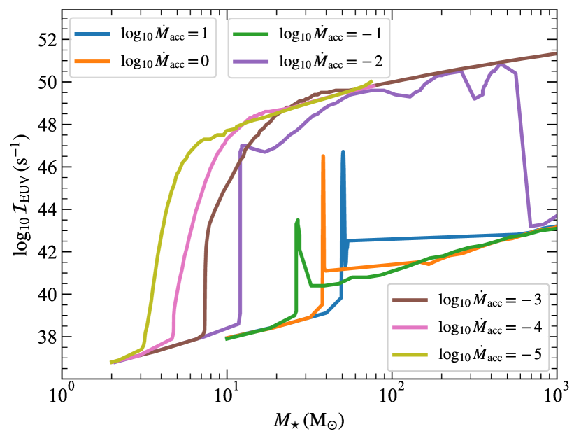
Figure 1: Ionizing rate (in per s) of EUV photons in the energy range $13.6\,\rm{eV}-\infty$ as a function of the protostellar mass, for different mass accretion rates in the GENEVA Population III stellar evolution models used in this work (Haemmerlé et al., 2018). Lower accretion rates lead to higher effective temperatures, thus producing more ionizing photons.

We insert a sink particle at the maximum level of refinement once the density exceeds $10^{13}\,\rm{cm^{-3}}$; the sink particle formation criteria is described in detail in Federrath et al. (2010b, 2011b). The sink particle can move around the grid, and accrete mass from its surroundings, with the sink accretion radius set to 2.5 cells at the highest level of refinement to avoid artificial fragmentation very close to an existing sink.

2.3 Magnetic fields

It is now well known that magnetic fields can be exponentially amplified in turbulent environments due to the action of turbulent dynamo (see the review by Subramanian, 2019). However, reaching numerical convergence while resolving the action of turbulent dynamos is not currently possible given the high Reynolds numbers in the ISM. Nonetheless, previous works find that as long as the collapsing cloud is resolved with at least 32 cells per Jeans length, dynamo amplification of magnetic fields can be captured (Federrath et al., 2011c; Turk et al., 2012; Schober et al., 2012b).

Numerous works point out that it is plausible for a seed field to be present during the formation of the first stars (Sharda et al., 2020, and references therein). Following the results of Sharda et al. (2021) who find that even an initially week seed field is quickly amplified to saturation due to the action of small-scale turbulent dynamo, we set our initial magnetic field strength to $30\,\mathrm{\mu G}$, which corresponds to a saturation state where the magnetic energy is 10 per cent of the turbulent kinetic energy (Federrath et al., 2011a, 2014; Federrath, 2016; Schober et al., 2015), appropriate for trans-sonic Mach numbers and near-unity Prandtl numbers as expected in the early Universe (Haugen et al., 2004; Brandenburg & Subramanian, 2005). The power spectrum of magnetic fields goes as $P_{\mathrm{mag}}\propto k^{1.5}$ for $2\leq k\leq 20$. The initial seed field is completely turbulent, since the field is not expected to be ordered prior to the formation of the first stars in the minihalo.

2.4 Protostellar evolution

To model the evolution of stellar radius, effective temperature, and luminosity in the protostellar phase, we use the stellar evolution models of Haemmerlé et al. (2018). The models are calculated using a modified version of the 1D GENEVA stellar evolution code (Eggenberger et al., 2008) that solves for the structure of the stellar interior by taking the protostellar accretion rate into account (Haemmerlé et al., 2013, 2016). The GENEVA grid spans across a wide range of protostellar masses ($2-10^{4}\,\rm{M_{\odot}}$) and accretion rates ($10^{-5}-10\,\rm{M_{\odot}\,yr^{-1}}$) that we interpolate across to obtain the stellar radius ($R_{\star}$) and effective temperature ($T_{\rm{eff}}$). If the accretion rate falls outside the range considered in the GENEVA model grids, we use the closest value of the stellar properties of interest that are available in the model grid (e.g., Jaura et al., 2022). We then use these quantities to estimate the radiative outputs from our stars.

2.5 Ionizing radiation feedback

To model the radiation transport of ionizing photons from our star particles we use the VETTAM radiation (magneto-)hydrodynamics (RMHD) scheme (Menon et al., 2022), and fully couple the photoionization to our primordial chemistry network; the details of this numerical approach (and tests) will be presented in a forthcoming paper (Menon & Sharda, 2024); we only mention the salient features relevant to our study here. VETTAM uses the Variable Eddington Tensor closure by computing the Eddington tensor with a non-local ray-tracing approach, and uses this to close the system of RMHD equations; this non-local approach permits significantly higher accuracy in the radiation transport than methods that use local closure relations – such as flux limited diffusion (FLD) or the Moment-1 (M1) closure – especially in the presence of multiple radiation sources as in a star cluster (see, for example, Fig. 13 in Menon et al., 2022). To the best of our knowledge, this is the only suite of RMHD simulations that use VET based radiation hydrodynamics and is fully coupled to chemistry.

VETTAM uses an implicit global temporal update for the radiation moment equations for each band, including the radiative output from sink particles as a smoothed Gaussian source term in the moment equations that has a form

$$\mathcal{J}_{*}(r)=\frac{L_{*}}{\left(2\pi\sigma_{*}^{2}\right)^{3/2}}\exp\left(-\frac{r^{2}}{2\sigma_{*}^{2}}\right),$$ (1)

where $L_{*}$ is the luminosity in the given energy band, $r$ is the radial distance of a grid cell from the sink particle, and $\sigma_{*}=2\Delta x_{\mathrm{min}}$, where $\Delta x_{\mathrm{min}}$ is the minimum cell size in the domain To compute $L_{*}$, we obtain (interpolated) values for the stellar radius ($R_{*}$) and temperature ($T_{*}$) from our (subgrid) stellar evolution model using its instantaneous mass and accretion rates from the simulation, and assume the star radiates as a blackbody. This permits us to calculate $L_{*}$ as

$$L_{*}=4\pi R_{*}^{2}\int_{\nu_{\mathrm{min}}}^{\nu_{\mathrm{max}}}B_{\nu}(T_{*})d\nu,$$ (2)

where $\nu_{\mathrm{min}}$ and $\nu_{\mathrm{max}}$ are the frequency limits of the two radiation bands that we evolve: one from $13.6\,\rm{eV}-15.2\,\rm{eV}$ that can only ionize H, and another from $15.2\,\rm{eV}-\infty$ that can ionize both H and H₂. We can then estimate the rate of ionizing photons, $\mathcal{I}_{\nu}$, from the star as

$$\mathcal{I}_{\nu}=4\pi R_{*}^{2}\int_{\nu_{\rm{min}}}^{\nu_{\rm{max}}}\frac{B_{\nu}(T_{*})}{h\nu}d\nu\,.$$ (3)

We will refer to $\mathcal{I}_{\nu}$ for the energy band ionizing H as $\mathcal{I}_{\rm{EUV}}$. Figure 1 plots $\mathcal{I}_{\rm{EUV}}$ as a function of the protostellar mass for different accretion rates, $\dot{M}_{\rm{acc}}$. Higher $\dot{M}_{\rm{acc}}$ makes the star bloat up, which reduces the effective temperature and brings down $\mathcal{I}_{\rm{EUV}}$. All the tracks plotted in Figure 1 are almost identical to those from Hosokawa & Omukai (2009) and Hosokawa et al. (2010) using a different stellar evolution code, except for the one for $\dot{M}_{\rm{acc}}=0.01\,\rm{M_{\odot}\,yr^{-1}}$.

For each radiation band, we perform the radiation transport independently, and compute the photoionization rate using the absorbed radiation energy density in a cell, which we pass on to KROME for the photochemical reactions

$$\mathrm{H}+\gamma \rightarrow\mathrm{H}^{+}+\mathrm{e}^{-}$$ (4)

$$\mathrm{H}_{2}+\gamma \rightarrow\mathrm{H}+\mathrm{H},$$

Note that for $\mathrm{H}_{2}$, we make the assumption that the photoionized product, ${\mathrm{H}^{+}_{2}}$, rapidly undergoes dissociative recombination (due to its high reaction rate in dense ionized gas), resulting in the production of two hydrogen atoms. This quasi-dissociation approach for the outcome of $\mathrm{H}_{2}$ ionization has also been invoked in other works (e.g., Jaura et al., 2022). We also incorporate heating due to photoionization of these species in the thermal balance computed by KROME. The thermal energy deposited in the gas per photoionization is computed from the excess energy available per photoionization event, which depends on the stellar spectrum as follows

$$\mathcal{E}_{\nu}=\frac{\int_{\nu_{\mathrm{min}}}^{\nu_{\mathrm{max}}}\left(B_{\nu}(T_{*})\sigma_{\nu}h(\nu-\nu_{0})/h\nu\right)\,d\nu}{\int_{\nu_{\rm{min}}}^{\nu_{\rm{max}}}\left(B_{\nu}(T_{*})\sigma_{\nu}/h\nu\right)\,d\nu}.$$ (5)

We will refer to $\mathcal{E}_{\nu}$ for the energy band ionizing H as $\mathcal{E}_{\rm{EUV,H}}$ and that ionizing H₂ as $\mathcal{E}_{\rm{EUV,H_{2}}}$. In the presence of multiple stars, we use the luminosity-weighted average of $\mathcal{E}_{\nu}$ over all the stars. Following Osterbrock (1989), we specify the frequency-dependent cross section of H as

$$\sigma_{\rm{H}}=6.3\times 10^{-18}\left(\frac{\nu}{13.6\rm{eV}/h}\right)^{-3}\,.$$ (6)

We follow Baczynski et al. (2015) to express the frequency-dependent cross section of H₂ ($\sigma_{\rm{H_{2}}}$) as a step function between $15.2-18.1\,\rm{eV}$, and assume it falls off as $\nu^{-3}$ for higher energies. This formulation is based on analytical work by Liu & Shemansky (2012), and is consistent with experimental results to within 20 per cent (Chung et al., 1993).

We also include the effect of the radiation pressure on gas by depositing the momentum carried by ionizing photons that are absorbed. We invoke on-the-spot approximation for photons emitted via recombination of H⁺ to the ground state, assuming that they are reabsorbed before they can travel far from their production sites (e.g., Baker & Menzel, 1938; Osterbrock, 1989).

We do not track the ionization of other species (like D, HD and He) due to stellar photons since He remains relatively inert and the mass fractions of D and HD are orders of magnitude less than H and H₂. We also do not include the effects of far-ultraviolet Lyman-Werner (LW) radiation emitted by stars which can photodissociate H₂ (e.g., Hosokawa et al., 2011; Baczynski et al., 2015; Jaura et al., 2022; Sugimura et al., 2023); earlier studies have shown that the effects of this is rather minor (Hosokawa et al., 2016; Jaura et al., 2022). That being said, some studies suggest that the heating from photodissociation could affect the accretion rates onto stars (Susa et al., 2014; Stacy et al., 2016). We will present calculations with the LW band included in an upcoming paper.

2.6 Multiple turbulent realizations

The lack of efficient cooling agents (i.e., metals and dust) render Population III star formation more prone to fragmentation over a larger range in density as compared to Population I star formation (e.g., Prole et al., 2023). This is further complicated by the fact that the outcomes of star formation in cloud cores are stochastic in nature due to the presence of turbulent fluctuations (Sharda et al., 2020, figure 7). Therefore, it is insufficient to run a single suite of simulations with a particular random seed and conclude a statistically significant result (Goodwin et al., 2004a, b; Wollenberg et al., 2020). Further, Sharda et al. (2020) highlight how the impact of magnetic fields on the Population III IMF cannot be ascertained by running only a few simulations, since the initial random fluctuations caused by turbulence can significantly alter the resulting stellar masses from one simulation to the next. This complication is not limited to star formation – recent works on cosmological simulations also find that stochasticity leads to significant scatter in the outcome for identical initial conditions (Davies et al., 2022, 2024; Borrow et al., 2023).

To balance the stochasticity of outcomes and computational feasibility, we conduct 3 turbulent realizations for each subcategory of simulations (HD, MHD, RHD and RMHD), where each realization uses the same set of (pseudo-)random seeds to generate the initial turbulent velocity and magnetic fields. This is sufficient for our purposes since our aim here is not to derive an IMF (that would otherwise require $\gtrsim 12$ realizations). In Section 3, we first present and discuss the results for a set of simulations that mostly formed only one star by the time we stop the simulations. This particular set of simulations is easier to analyze since gas dynamics around the star are not impacted by fragmentation. In Section 4, we then describe the evolution of the other two realizations of the RHD and RMHD simulations where we find widespread fragmentation and formation of Population III star clusters.

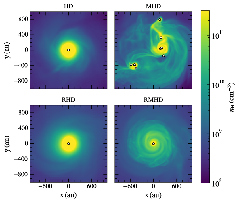
Figure 2: Face-on density-weighted projections through the $\hat{z}$ axis of the gas number density at the end of the simulations. The four panels correspond to the runs with hydrodynamics (HD), magneto-hydrodynamics (MHD), radiation-hydrodynamics that includes ionizing radiation feedback (RHD), and radiation-magnetohydrodynamics (RMHD). White dots represent the position(s) of sink particle(s), used as a proxy for Population III stars. All except the MHD run only produces a single star. The accretion disk around the star in the RMHD simulation is less dense as compared to the other simulations. The mass of the central star is $120\,\rm{M_{\odot}}$ (HD), $60\,\rm{M_{\odot}}$ (MHD), $110\,\rm{M_{\odot}}$ (RHD), and $57\,\rm{M_{\odot}}$ (RMHD).

3 Results and discussion

We evolve the simulations until 5000 yr post the formation of the first star. We first present and discuss results for the simplest turbulent realization, which only produces a single Population III star in the HD, RHD, and RMHD runs but shows fragmentation in the corresponding MHD run. This set of simulations is easy to follow because (except for the MHD case) it produces a single star with a well-defined accretion disk around it and makes the comparison between them straightforward. We first show and contrast the evolution of thermodynamic quantities (density, temperature, and mass fraction of H₂) in the four subsets of simulations, and then move on to the properties of magnetic fields and ionizing feedback and how their interplay governs gas fragmentation, star formation and accretion. Movies associated with the evolution of various parameters of interest are available as supplementary (online only) material.

3.1 Physical and chemical properties

Figure 2 plots the density-weighted projections of the number density of the gas within a $0.01\,\rm{pc}$ region centered on the star (center of all stellar masses for the MHD run), at the end of the simulations. We see that the HD, RHD, and RMHD runs all yield a single massive star with a well-defined accretion disk around it. The disk is geometrically thin when viewed along the edge-on axes (see the movies in the supplementary material). It is also clear that the accretion disk is denser in the HD and RHD runs, as compared to the RMHD run. The MHD run fragments to produce a cluster of 12 stars.

The differences between the HD and the RHD runs are more prominent in the temperature structure around the star, as we read off from Figure 3. The RHD run contains an inner region that is colder than the HD run, which at first glance might seem counter-intuitive. Closer inspection reveals that this outcome is a result of radiation pressure acting on the gas in the immediate vicinity of the star that slows down the rate of (radial) gas infall, which weakens the shock produced by the flow. We find that the radial velocity of the gas in and around this region is trans-sonic and lower in the RHD run by a factor $\gtrsim 4$ in comparison to the HD run, where the flow is supersonic. This difference manifests in the higher shocked temperatures (and associated dissociation of molecular hydrogen) in the HD run. This is also why we observe enhanced levels of molecular hydrogen in the inner disk in the RHD run (see Figure 4). In both the HD and RHD runs, the hot gas ($T>5000\,\rm{K}$) all throughout the projection window is a consequence of the dependence of gas cooling on the Jeans resolution in the presence of accretion shocks created by matter falling onto the disc. As Sharda et al. (2021, appendix A) explain, if the Jeans length is well resolved, the dissociation timescale for molecular hydrogen in the post-shock region is smaller than the (resolved) gas cooling timescale, which ensures that H₂ dissociates faster than the gas can cool, thus giving rise to high gas temperatures. As we will explore below, this effect of the Jeans resolution on the chemistry is more crucial than protostellar radiation effects throughout the duration of the simulations. The high temperatures caused by shocks also enhance the mass fraction of H⁺ in the HD and RHD runs, as we see from the projections of the mass fraction of H⁺ we plot in Figure 5. We notice the presence of a partially ionized H ii region close to the star, which is not seen in runs without ionizing feedback. The average mass fraction of H⁺ within the region is $\sim 10^{-3}$, which implies that they are only marginally ionized, unlike fully ionized H ii regions (e.g., Ferland et al., 1998; Kewley et al., 2019). The H ii region is unable to expand for the duration of these simulations. We will explore this further in Section 3.3 and Section 4.

Perhaps the most striking feature in the temperature maps is the presence of large amounts of cold gas around the star(s) in runs including magnetic fields (MHD and RMHD). This feature is also noticeable in earlier MHD simulations of Population III star formation (Sharda et al., 2020, 2021; Saad et al., 2022; Stacy et al., 2022), and cosmological simulations that use high Jeans resolution (Turk et al., 2012; Díaz et al., 2024). This occurs because magnetic fields slow down gas compression by providing pressure support to the gas, which in turn brings down the rate of compressional heating (e.g., Saad et al., 2022). Lower temperatures lead to a larger abundance of molecular H₂ in the MHD and RMHD runs, as shown in Figure 4. The RMHD run is slightly different from the MHD run in that the former contains hot gas in the immediate vicinity of the star because of ionizing feedback. The gas farther out from the star in the RMHD is cold – as it is shielded from the stellar radiation – but also less dense, so it cannot fragment. This partially explains why the MHD run fragments to form more than one star but the RMHD run does not (see also, Section 3.4). However, we cannot comment on whether this effect is always present based on a single turbulent realization; in fact, as we will see in Section 4, other RMHD realizations show widespread fragmentation.

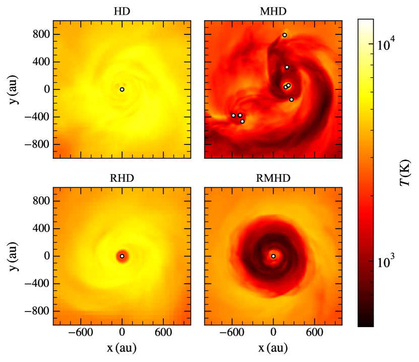
Figure 3: Same as Figure 2 but for the density-weighted gas temperature. The accretion disk is much colder in runs including magnetic fields (MHD and RMHD).

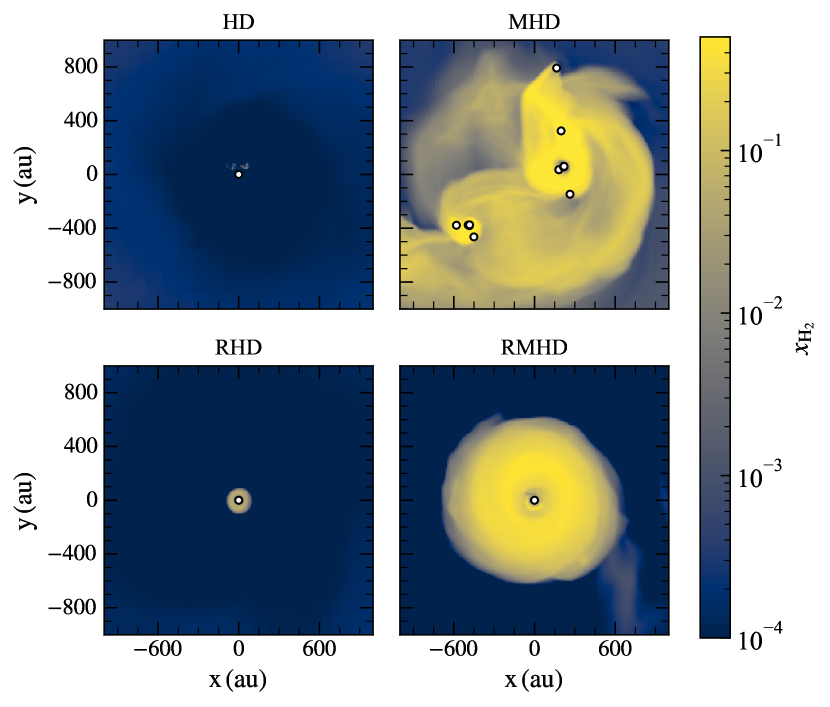
Figure 4: Same as Figure 2 but for the density-weighted mass fraction of molecular hydrogen. The accretion disk is highly molecular in the runs including magnetic fields (MHD and RMHD).

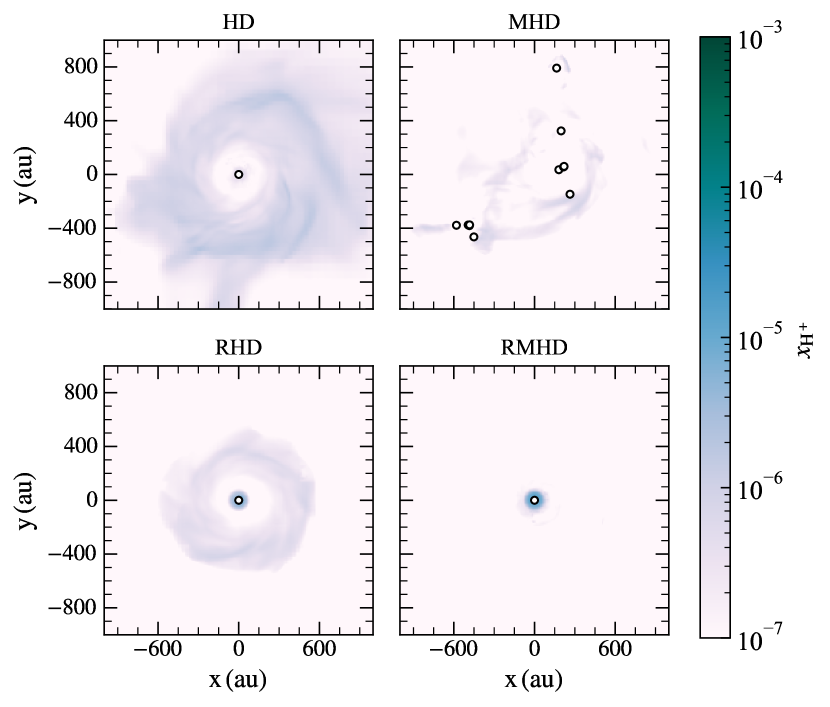
Figure 5: Same as Figure 2 but for the density-weighted mass fraction of H⁺. The impact of ionizing feedback is noticeable close to the star in the RHD and RMHD runs, where $x_{\rm{H^{+}}}$ is higher. The large scale diffuse $x_{\rm{H^{+}}}$ seen in the HD and RHD runs is a result of hydrodynamic shocks.

3.2 Radial and polar profiles

We now look at the radial and polar profiles of key physical parameters in the four simulations. The profiles in the MHD run at the end of the simulation are more complex and difficult to interpret, owing to fragmentation. Therefore, we analyze the profiles for all four runs at an earlier time – $\approx 1500\,\rm{yr}$ after the (first) star forms – prior to fragmentation in the MHD run. We verify that analyzing the profiles at an earlier time does not make a big difference for our purposes since the profiles are fairly constant in the other three runs at later times.

Figure 6 plots the mass-weighted (cylindrical) radial and polar profiles of gas density, temperature, and mass fractions of H₂ and H⁺. For the purposes of this discussion, we classify the inner accretion disk as the region within $100\,\rm{au}$ of the star, and outer accretion disk as the region between $100-500\,\rm{au}$ from the star. Figure 6 shows that the radial density profiles in the inner accretion disc are very similar between all the runs, but the MHD and RMHD runs contain somewhat denser gas in the outer accretion disc at this epoch. In the polar direction, the HD, RHD, and MHD runs show a density profile that peaks near $z=0$ and smoothly decline in either direction. On the other hand, the polar density profile in the MHD run is much flatter, indicating the presence of uniform high density gas all around the sink. It is therefore not surprising that the MHD run fragments past this point.

The temperature profile in the inner disc is quite distinct in all the four runs, and are set by distinct physics. The high temperature near the star in the HD run is a consequence of coupled chemistry and cooling, which can occur due to the high Jeans resolution we achieve in our simulations, as we explain in Section 3.1. The temperature is lowest in the MHD run due to magnetic fields reducing compressional heating, low enough to trigger fragmentation and formation of multiple stars. The somewhat lower temperature in the RHD run compared to the HD run is due to ionization – recombination balance that produces H which then forms H₂ via three-body reactions. There is a possibility that some of this H₂ will be dissociated into H again due to LW photons, which we do not consider in this work. Finally, the temperature in the RMHD run in the inner disc is set by a mixture of all the three above: Jeans resolution, ionization – recombination balance, and magnetic fields. Overall, the effect of magnetic fields seem to be the strongest, since the temperature in the RMHD run is closest to the MHD run.

As expected based on the temperature profiles and results in Section 3.1, the MHD and RMHD runs contain a significant amount of H₂ in the inner disc. The temperature in the RMHD run is high enough to cause some H₂ dissociation, which slightly lowers the mass fraction of H₂ as compared to the MHD run. The RHD run also contains a non-negligible amount of H₂ in the inner disc, whereas the HD run has no discernible H₂. The findings are qualitatively similar in the polar direction as well: the MHD and RMHD runs have a high fraction of H₂, and the RHD run has non-negligible H₂ close to the star. The last panels of Figure 6 clearly show an enhancement in the fraction of H⁺ close to the star in the runs including ionizing feedback (RHD and RMHD). Nevertheless, the mass fraction of H⁺ is negligible, as we explore further in Section 3.3 below.

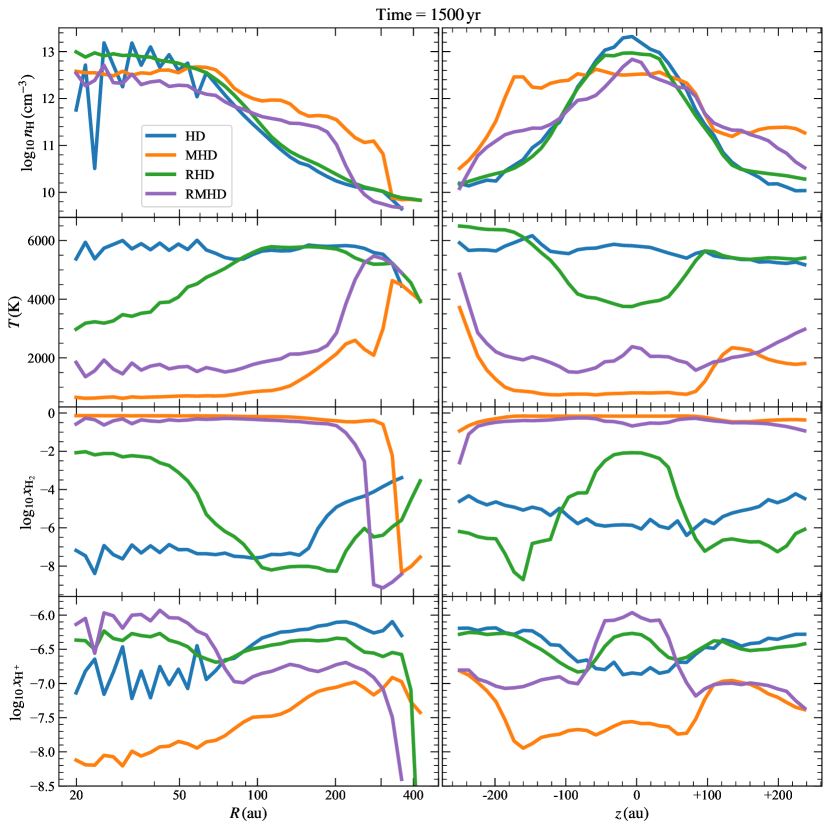
Figure 6: Left panel: mass-weighted radial profiles in the accretion disk of the gas number density, temperature, and mass fractions of H₂ and H⁺ in the four simulations. The profiles for all the simulations are plotted prior to fragmentation in the MHD run, which occurs $1500\,\rm{yr}$ after the formation of the first star. The RMHD run exhibits lower temperatures, higher mass fractions of H₂ and lower densities as compared to the RHD run. Ionization of H is most noticeable close to the star where there is an overabundance of H⁺ as compared to the control (HD) run. Right panel: Same as the left panel but for profiles in the polar direction.

3.3 Evolution of H ii regions

We have seen in Section 3.1 and Section 3.2 that the impact of radiation on the evolution of the clouds is quite modest. This is primarily because the stars are unable to ionize the dense gas in vicinity of stars, and only forms a partially ionized H ii region. This can also be seen in the radial profiles of the mass fraction of H⁺ (cf. Figure 6), which, while higher than the control run without radiation, are still quite low: $x_{\rm{H^{+}}}\lesssim 10^{-6}$. The weak effect of radiation can be understood by comparing the ionizing photon rates to the gas densities by computing the size of the Stromgren sphere that could be driven (Strömgren, 1939). If the Stromgren radius is much smaller than the cell size, it implies that the photon rate is insufficient to ionize the cells in the vicinity of the source, and can only partially do so. The Stromgren radius for an ionized hydrogen bubble under the on-the-spot approximation is given by

$$R_{\mathrm{St}}=\left(\frac{3\mathcal{I}_{\rm{EUV}}}{4\pi\alpha_{\mathrm{B}}n_{\mathrm{H}}^{2}}\right)^{3}\sim 0.1\,\mathrm{au}\,\left(\frac{\mathcal{I}_{\rm{EUV}}}{10^{49}\,\mathrm{s}^{-1}}\right)^{1/3}\left(\frac{n_{\mathrm{H}}}{10^{12}\,\mathrm{cm}^{-3}}\right)^{2/3}$$ (7)

where $n_{\mathrm{H}}$ the hydrogen number density and $\alpha_{\mathrm{B}}$ the case-B recombination coefficient; in the dimensional scaling above, we have used the values for $\mathcal{I}_{\rm{EUV}}$ and $n_{\mathrm{H}}$ that we find for our Population III star and its vicinity respectively, and the value of $\alpha_{\mathrm{B}}$ from Hui & Gnedin (1997) appropriate for a temperature of $10^{4}$K. The value reported above is smaller than the cell size of our simulations, explaining why we do not fully ionize cells close to the star. Note that this does not mean that if we had higher resolution then the star would have drive an ionized bubble – the densities one would resolve would also be higher in this case, and the same problem would likely occur. This is rather a statement on the weak ionizing luminosities of the star for the densities with which it is surrounded. We also do not see any expansion of the H ii region in the polar directions where the densities are lower and the Stromgren radius can be resolved in our simulations. This is because of the relatively high accretion rates, which have the effect of reducing $\mathcal{I}_{\rm{EUV}}$ (cf. Figure 1; Hosokawa & Omukai 2009; Hosokawa et al. 2013).

The calculation above implies that $\mathcal{I}_{\rm{EUV}}$ needs to increase and $n_{\mathrm{H}}$ needs to decrease for effectively driving a H ii region. This is highly likely to occur at later times as the star becomes more massive and emits more ionizing photons, while $n_{\mathrm{H}}$ decreases as mass is increasingly depleted in the vicinity of the star – especially in the polar directions. Another, more subtle effect could arise from the evolution of the mass accretion rate onto the star. In the absence of any gas infall onto the minihalo, the accretion rate onto the star would naturally lower with time as the disk/cloud gets increasingly depleted, and any fragmentation would decrease the accretion rate onto the primary star further due to competitive accretion. In fact, in agreement with our expectations, other RHD simulations of Population III star formation in the literature find that H ii regions are driven at times $\gtrsim 15000\,\mathrm{yr}$ (Hosokawa et al., 2016; Sugimura et al., 2020; Jaura et al., 2022), while the effects at earlier times are modest. We will be well placed to comment on these effects in a forthcoming paper where we follow the evolution of the simulation for significantly longer times.

We note that Jaura et al. (2022) report that H ii regions in their simulations are trapped in the disk, and therefore do not have a significant effect on the system. We pause to clarify that the physical reason there is distinct from what is described above. In their work, they do ionize the cells in the close vicinity of the star since they 1.) evolve for much longer times, and 2.) have an effective grid resolution $\lesssim 1\,\mathrm{au}$. However, this ionized bubble is unable to undergo a (D-type) pressure-driven expansion, even in the polar directions, and remains trapped within the disk – unlike several other works in the past (see Table 4 in Jaura et al., 2022). This occurs because the gravitational influence of the star is so strong such that the ionized gas is unable to expand. We cannot comment on this possibility in this work since our ionizing luminosities at the times we evolve are too weak to even produce an ionized bubble (i.e., the Stromgren sphere) that we resolve.

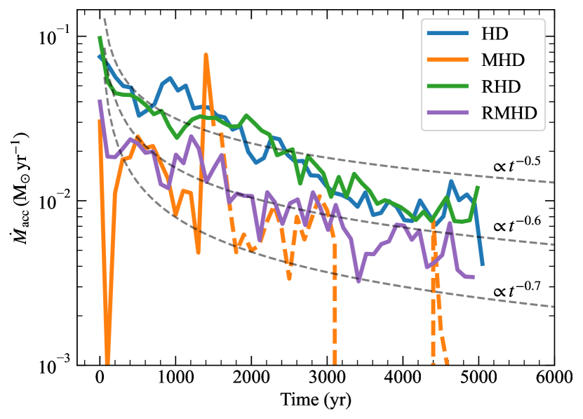
Figure 7: Average mass accretion rates onto the protostar (in case of MHD, the oldest and most massive protostar) in the four simulations. Fragmentation in the MHD run occurs at $1500\,\rm{yr}$ after the formation of the first star, which is indicated by the onset of the dashed orange curve, to emphasize that the star does not evolve in isolation thereafter. Simulations including magnetic fields (MHD and RMHD) exhibit lower protostellar accretion rates. Dashed grey curves show example trends for $\dot{M}_{\rm{acc}}\propto t^{-\beta}$, with $\beta=0.5,0.6,0.7$, as shown on the plot.

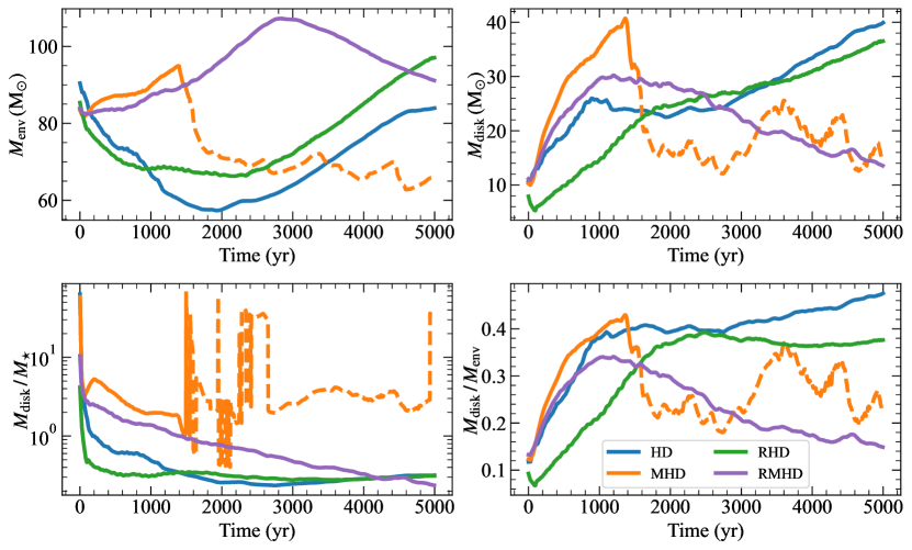
Figure 8: Sequence of mass transport from the largest to smallest scales. Top left panel: Evolution of mass enclosed within an envelope of radius $0.01\,\rm{pc}$ centered at the location of the star (in the HD, RHD, and RMHD simulations) and at the location of the most massive star in the MHD simulation. The MHD run fragments $1500\,\rm{yr}$ after the formation of the first star, shown by the dashed orange curve. Top right panel: Same as the top left panel but for the accretion disc within $500\,\rm{au}$ of the star. Bottom right panel: ratio of mass in the disk to that in the envelope. Bottom left panel: ratio of mass in the accretion disc to the protostellar mass. At each successive stage (from larger scales to the protostar), magnetic fields slow down mass transport, ultimately leading to lower stellar masses in the MHD and RMHD simulations (cf. Figure 9).

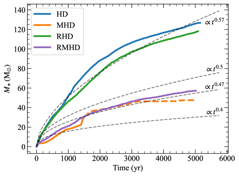
Figure 9: Mass growth of the formed single protostar (in case of MHD, the oldest and most massive protostar) in the four simulations. Fragmentation in the MHD run occurs at $1500\,\rm{yr}$ after the formation of the first star; this is indicated by the onset of the dashed orange curve to emphasize that the star does not evolve in isolation thereafter. Dashed grey curves demarcate example trends to guide the eye for the relation $M_{\star}\propto t^{\gamma}$ with $\gamma=0.57,0.50.47$ and $0.4$. Lower accretion rates in the MHD and RMHD runs lead to lower stellar masses (by a factor $\gtrsim 2$) as compared to the HD and RHD runs.

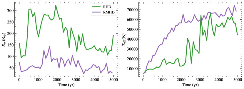
Figure 10: Temporal evolution of stellar properties based on the GENEVA stellar structure models (Haemmerlé et al., 2018), using the instantaneous mass and accretion rates of the star, compared between the RHD and RMHD runs. Left panel: stellar radius. Right panel: effective temperature. The star in the RMHD run is more compact and bluer than that in the RHD run even though its mass is less by a factor of two.

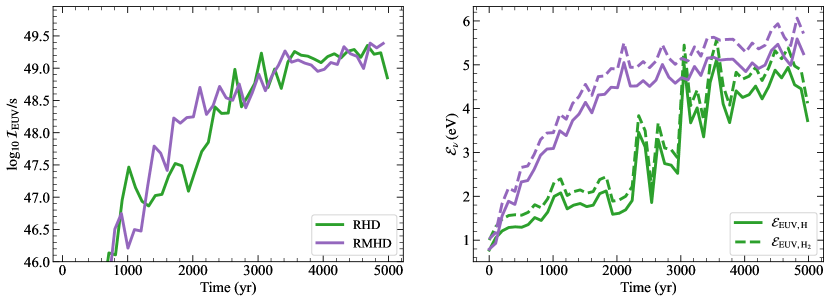
Figure 11: Left panel: Ionizing rate (in per s) of EUV photons in the energy range $13.6\,\rm{eV}-\infty$ from the central protostar as a function of time for the RHD and RMHD runs. Right panel: Heat released per ionization, $\mathcal{E}_{\nu}$, in the two runs. Solid curves are for ionization of H (energy range $13.6\,\rm{eV}-\infty$) whereas dashed curves denote ionization of H₂ (energy range $15.2\,\rm{eV}-\infty$). Lower accretion rates in the RMHD case lead to hotter and more compact stars, leading to a larger $\mathcal{E}_{\nu}$ as compared to the RHD case.

3.4 Accretion disks and mass transport

Having looked at the physical and chemical properties of the gas around the stars, we now turn to the accretion rates of the stars that form in the simulations and the physics behind it, which is crucial for interpreting the properties of the formed stars (Section 3.5). We first look at the accretion rates of the isolated stars in the HD, RHD, and RMHD runs, and that of the oldest and most massive star in the MHD run. Figure 7 plots the temporal evolution of the accretion rate averaged over $100\,\rm{yr}$ intervals for the different runs. All the accretion rates are quite high in the first $1000\,\rm{yr}$, and decline as time progresses; the accretion rate in the RMHD run approximately declines with time as $\dot{M}_{\rm{acc}}\propto t^{-0.6}$ for the duration of the simulation.

Interestingly, the long-lived accretion burst in the MHD run at $t\approx 1500\,\rm{yr}$ is followed by the onset of fragmentation, as we show via the dashed orange curve in Figure 7. There is also a clear difference between runs that include magnetic fields and those that do not: both the MHD and RMHD runs exhibit lower accretion rates than the HD and RHD runs by a factor of few at all times. In fact, the most massive star in the MHD run undergoes multiple periods of quiescence due to fragmentation. As we shall see later in Section 3.5, this has significant consequences for the masses of the stars that form in the presence of magnetic fields.

To further understand why the accretion rates onto the star are lower in runs with magnetic fields, we look at the temporal evolution of the available mass budget over multiple scales that supply mass to the star. The top left panel of Figure 8 plots the mass within the envelope that constitutes a spherical region of radius $0.01\,\rm{pc}$ centered on the star; this envelope feeds the accretion disk of the star via infalling gas. We see from these panels that the amount of mass reaching the envelope initially increases in the MHD and RMHD runs, but then turns over and starts to decline. In contrast, the rate of mass transfer from the envelope to the accretion disk is initially quite fast in the HD and RHD runs, resulting in a decline of mass in the envelope and buildup of mass in the disk, as we see from the top right panel of Figure 8. This mass is consequently accreted by the star at a high rate. Since the mass of the star is initially small, the ratio $M_{\rm{disk}}/M_{\star}$ is high (cf. bottom left panel of Figure 8). We learn that magnetic fields limit the amount of gas infalling onto the envelope at later stages, leading to mass depletion within the accretion disk. However, in addition to this, the rate of mass transport from the envelope to the disk also declines in the presence of magnetic fields, as we show in the bottom right panel of Figure 8. There is no further fragmentation in the HD, RHD and RMHD runs because the mass in the disk continues to accrete efficiently onto the central star, thereby ensuring $M_{\rm{disk}}/M_{\star}<1$. We demarcate the onset of fragmentation in the MHD run by dashed curves in all the panels. The mass transport from the disk to the star is so quick in the MHD run that the disk becomes $10\times$ as massive as the central star, and fragments. Subsequent peaks in $M_{\rm{disk}}/M_{\star}$ at late times mark the onset of further fragmentation within the accretion disk of the oldest star.

To summarise, the mass growth of the stars in our simulations are governed by the rate of mass transfer from larger scales onto the envelope, envelope to the accretion disk, and accretion disk to the star. At each stage of mass transfer, magnetic fields significantly influence the outcome and the total mass budget available. We also learn that, in addition to this transport, fragmentation is governed by whether the accretion disk becomes too massive as compared to the central star (i.e., $M_{\rm{disk}}/M_{\star}\gg 1$). This can occur if the accretion rate onto the star is small, for example, due to protostellar feedback or negative feedback from fragmentation itself.

3.5 Stellar properties

3.5.1 Stellar mass

Next, we look at the evolution of stellar mass of the stars formed in the four runs in Figure 9. We plot the mass growth curve for the oldest and the most massive star in the MHD run. The stellar mass growth in the MHD and RMHD runs closely track each other, and are substantially slower as compared to the HD and RHD runs. In the HD and RHD runs, we find that the mass growth roughly follows $M_{\star}\propto t^{0.57}$ whereas in the MHD and RMHD runs, it follows $M_{\star}\propto t^{0.47}$. At the time we stop the simulations, the stellar masses in the four runs are: $127\,\rm{M_{\odot}}$ (HD), $48\,\rm{M_{\odot}}$ (MHD), $118\,\rm{M_{\odot}}$ (RHD), and $57\,\rm{M_{\odot}}$ (RMHD).

It is clear that magnetic fields have a dramatic impact on the stellar mass of Population III stars. It is noteworthy that within the first $5000,\rm{yr}$ of star formation, we already observe a twofold difference in the stellar mass between the RHD and RMHD runs. We also find that magnetic fields play a much more important role than ionizing feedback at the early epochs ($\lesssim 5000\,\mathrm{yr}$) of protostellar evolution that we simulate in this study. Ionizing feedback has a limited impact in lowering the stellar mass, even when we average accretion rates over some timescale to limit numerical noise in the stellar parameters (see Appendix A). If radiation feedback becomes dominant at later times, it will suppress mass growth of the star, further limiting the maximum mass a Population III star can acquire. This finding has major implications for the mass and the IMF of Population III stars, as we will explore in Section 5.

3.5.2 Stellar radius and effective temperature

The mass of a star and the accretion rates onto it affect the evolution of the properties of the protostar via the subgrid model we adopt (cf. Figure 1). This implies that the differences in these quantities (mass/accretion rates) we presented in previous sections would have direct consequences on the stellar properties, and thereby their radiative outputs. To investigate this, we study the evolution of the protostellar radius, $R_{\star}$, and effective temperature, $T_{\rm{eff}}$, in these runs. Figure 10 presents the results. We find that the star in the RMHD run is more compact and bluer than that in the RHD run, which can be attributed to its lower accretion rate (Figure 7). However, some of the variation we see in the stellar properties can be a result of the noise in the accretion rate, which depends on the grid resolution. A common approach to mitigate this issue is to average the instantaneous accretion rates over some timescale to suppress numerical noise (e.g., Stacy et al., 2016). We find that averaging the accretion rates this way to calculate stellar properties has a negligible impact (see Appendix A), and our finding that the RMHD run produces more compact and bluer stars holds regardless.

$R_{\star}$ and $T_{\rm{eff}}$ set the overall ionizing output and heating rate due to ionization. To explore the impact of more compact and bluer stars as in the RMHD run, we plot the rate of ionizing photons released, $\mathcal{I}_{\rm{EUV}}$, and associated thermal energy deposition in the gas per ionization event, $\mathcal{E}_{\nu}$, in the left and right panels of Figure 11 respectively. We find that there is no considerable difference in $\mathcal{I}_{\rm{EUV}}$ after $2500\,\rm{yr}$, but $\mathcal{E}_{\nu}$ is higher in the RMHD run for the entire duration of the simulation. This is not surprising since $\mathcal{I}_{\rm{EUV}}$ depends on both $T_{\rm{eff}}$ and $R_{\star}$ whereas $\mathcal{E}_{\nu}$ depends only on $R_{\star}$: larger $R_{\star}$ but lower $T_{\rm{eff}}$ in the RHD runs seems to counterbalance the lower $R_{\star}$ but higher $T_{\rm{eff}}$ in the RMHD ones. The larger heating in the RMHD run is partially responsible for rendering the gas in the immediate vicinity of the star hotter, as we see in Figure 6.

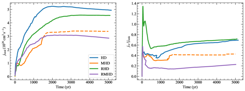
Figure 12: Left panel: specific angular momentum of the sink particle in the different simulations, as a function of time. Dashed orange curve marks the onset of fragmentation in the MHD run. Right panel: ratio of the specific angular momentum expected for the central star to that of the sink particle, as a function of time (see Section 3.5.3). This ratio indicates the fraction of angular momentum that the actual star can inherit from the sink particle. Magnetic fields redistribute angular momentum, and therefore lead to less angular momentum than in the case without magnetic fields. This will likely lead to Population III stars rotating at a smaller fraction of the breakup speed than anticipated.

3.5.3 Stellar rotation

Another quantity of interest we can infer from our simulations is the angular momentum budget of the protostars, which is fundamental to understanding whether Population III stars were fast rotators. This is important for a number of observational probes – most notably, strong rotation will induce mixing that can dredge up certain elements from the stellar interior to the surface (Yoon et al., 2012; Murphy et al., 2021; Jeena et al., 2023; Roberti et al., 2024; Tsiatsiou et al., 2024; Nandal et al., 2024), which can enrich the surrounding ISM via stellar winds or supernovae (e.g., Heger & Woosley, 2002, 2010; Ishigaki et al., 2018). Rotation also plays a key role in determining whether Population III stars produced gamma ray bursts (GRBs) at the end of their lifetime (e.g., Wang et al., 2012; Volpato et al., 2024). Almost all previous work on the rotation rate of Population III stars conclude that they were fast rotators, and rotated close to breakup speeds (see Hirano & Bromm 2018 for an exception).

Our simulations track the angular momentum budget of sink particles; however, we cannot directly interpret this as the angular momentum of the protostar, since the latter would be affected by gas dynamics at the sub-grid level. We follow the approach set out in Stacy et al. (2011) to estimate the fraction of angular momentum in the sink that will end up in the actual star. To do so, we calculate the time evolution of the specific angular momentum of an accreting star as

$$j_{\star}=\frac{\int^{t}_{0}\sqrt{GM_{\star}R_{\star}}\,\dot{M}_{\star}dt}{M_{\star}}\,,$$ (8)

where $R_{\star}$ and $M_{\star}$ are the radius and mass of the star. We make two key assumptions to perform this calculation: 1.) almost all the mass of the sink will end up in the star, so $M_{\star}\approx M_{\rm{sink}}$, and 2.) this mass transfer occurs via a (sub-grid) disc at the same accretion rate as that of the sink, so $\dot{M}_{\rm{\star}}=\dot{M}_{\rm{sink}}$. These assumptions permit us to adopt the values of $R_{\star}$ and $M_{\star}$ obtained with our sub-grid protostellar evolution model in equation 8. Defining $j_{\rm{sink}}$ to be the specific angular momentum of the sink, we use the ratio $j_{\star}/j_{\rm{sink}}$ to see how much of the sink angular momentum will be transferred to the star that we do not resolve in our simulations. We emphasize these assumptions are very crude. However, our purpose here is not to derive the rotation speed of the star (since, as Stacy et al. 2011 explain, conservation of angular momentum will lead to erroneously high rotation speeds, much more than the breakup speed), but to study the relative trends between the different simulations to understand whether physical processes like magnetic fields or ionizing feedback will change the angular momentum budget and thence the rotation speed.

Figure 12 plots $j_{\rm{sink}}$ and $j_{\star}/j_{\rm{sink}}$ as a function of time for the four simulations. We find that $j_{\rm{sink}}$ initially increases in all runs, as the angular momentum of the accreting material is added onto the sink. It eventually saturates (or starts mildly declining) as the accretion rates go down and the stellar mass goes up. It is also evident that $j_{\rm{sink}}$ is lower in the MHD and RMHD runs, owing to smaller central stellar masses and lower accretion rates. Moreover, we learn from the ratio $j_{\star}/j_{\rm{sink}}$ that a smaller fraction of the (already small) $j_{\rm{sink}}$ in the MHD and RMHD runs will likely end up in the star. This is well understood as a consequence of magnetic torques redistributing angular momentum in the disc, and slowing down the spin of the sink particles. Additionally, as we have seen in previous sections, the stellar radii are also smaller in runs with magnetic fields, which also reduces $j_{\star}$.

Thus, the overall impact of magnetic fields, as expected from semi-analytical models (Hirano & Bromm, 2018), is to slow down the rotation of Population III stars, similar to their role in setting the rotation rates of Population I stars. If Population III stars could eject material via protostellar outflows (Machida et al., 2006, 2008; Machida & Doi, 2013), the rotation rates would be even lower, as in Population I star formation (e.g., Jappsen & Klessen, 2004; Mathew & Federrath, 2021). However, the generation of strong large-scale mean field required for such outflows (e.g., via the large-scale $\alpha-\Omega$ dynamo – Pudritz 1981a, b; Brandenburg & Subramanian 2005) has not yet been conclusively shown in any existing Population III star formation simulations (e.g., Liao et al., 2019; Sharda et al., 2021).

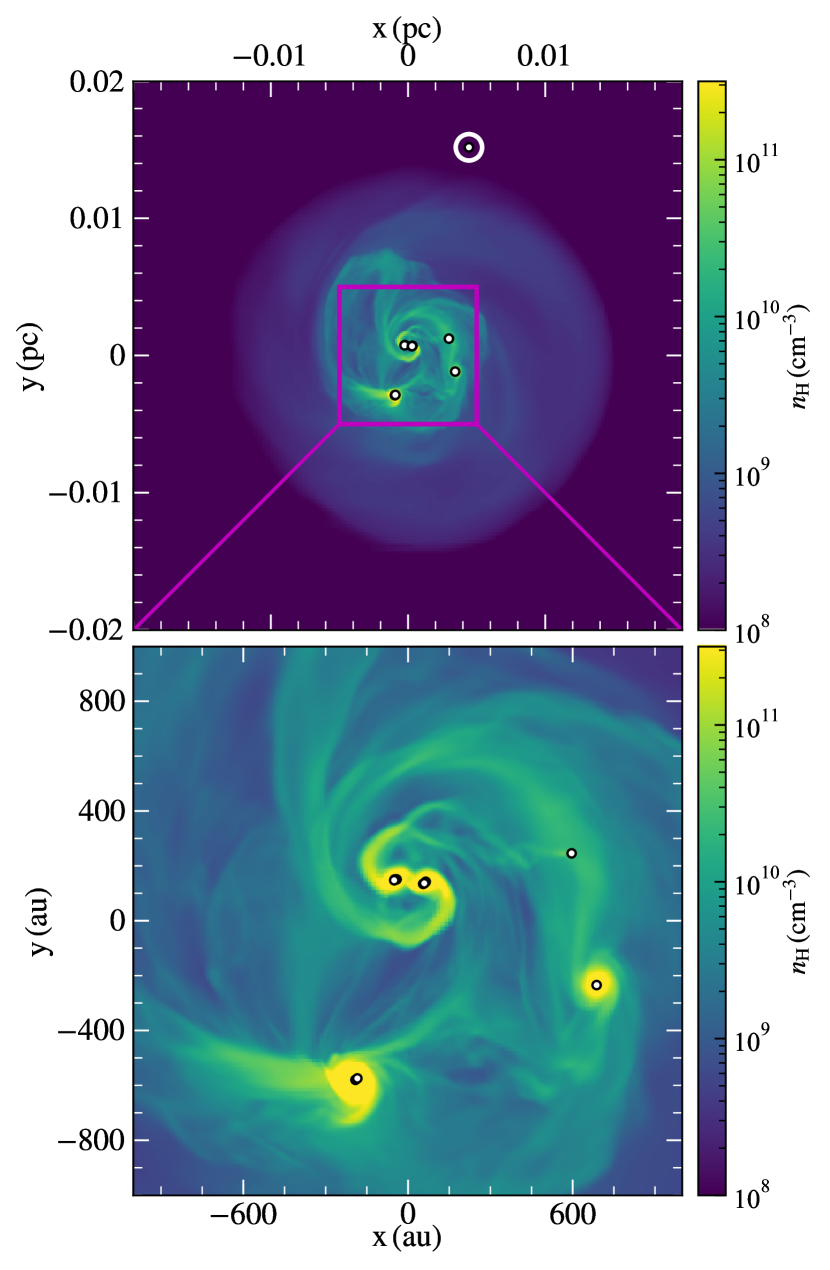
Figure 13: Top panel: density-weighted projection (along the $\hat{z}$ axis) of the gas density in one of the two turbulent RMHD realizations that fragment to produce Population III star clusters. White dots mark the position of all the stars. One of the (sub-Solar) mass stars is ejected from the cluster due to N-body interactions, as indicated by the white circle at its position. This star has a mass $0.45\,\rm{M_{\odot}}$, and stopped accreting after it was ejected. Bottom panel: zoom-in of the central $0.01\,\rm{pc}$ region that harbours the cluster of 11 stars. Several stars are unresolved in this plot as they are located very close to other stars. Multiple stars have their respective accretion disks interconnected via dense filamentary structures.

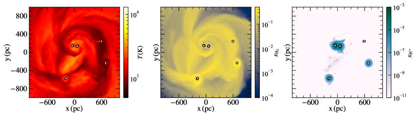
Figure 14: Same as the bottom panel of Figure 13 but for the density-weighted gas temperature, and mass fractions of H₂ and H⁺. Several stars in the cluster have partially ionized H ii regions around them, due to lower accretion rates. A vast majority of the gas remains molecular due to otherwise colder temperatures.

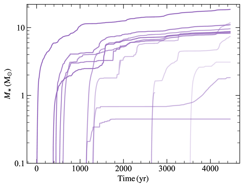
Figure 15: Mass growth of all the protostars in same RMHD run as in Figure 14. Progressively faded lines represent younger protostars, which can also be read off from the abscissa. The accretion rates for all stars are lower than the typical accretion rate seen in the isolated star run (cf. Figure 7). The $0.45\,\rm{M_{\odot}}$ star that gets ejected from the cluster by the end of simulation is born at $t\approx 1200\,\rm{yr}$. It stops accreting when it is ejected, at $t\approx 1700\,\rm{yr}$.

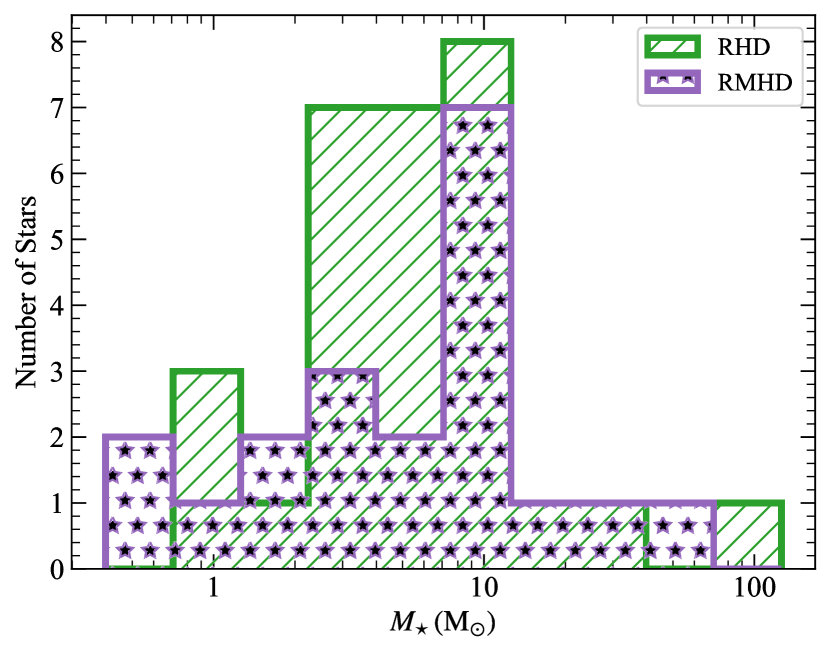
Figure 16: Mass distribution of stars in the three RHD (green) and RMHD (purple) turbulent realizations at the end of the simulations.

4 Evolution of Population III clusters

As we mention in Section 2, whether fragmentation will occur or not is sensitive to the turbulent realization used. Having looked at the simplest realization that (mostly) resulted in a single star, we now look at the evolution of stellar masses in the other RMHD realizations that produced star clusters. We only focus on the RMHD runs for this purpose, since it is the most physically realistic run.

Figure 13 and Figure 14 plot the density-weighted projections of the gas density, temperature and mass fraction of H₂, centered on the center of mass of all stars in one of the realizations. The zoom-in view of the central $0.01\,\rm{pc}$ of the cluster in Figure 13 shows how several stars are located very close to each other, but some stars are also located farther away in smaller, bound systems. We see the presence of cold, molecular gas throughout the central region, similar to that in the RMHD realization that produced an isolated star. The accretion disks of stars are interconnected via dense filamentary structures. This realization produces 12 stars within the first $5000\,\rm{yr}$ since fragmentation. The masses vary between $0.45-18.5\,\rm{M_{\odot}}$. The maximum mass is much lower than the first RMHD realization because of fragmentation-induced starvation that lowers the accretion rate onto the stars, as we read off from Figure 15. This is a well known outcome of fragmentation (e.g., Peters et al., 2010; Krumholz, 2011; Girichidis et al., 2012; Prole et al., 2022a; Sharda & Krumholz, 2022).

One implication of the low accretion rates is that the ionizing output from these stars is consistently higher as compared to the isolated stars we study above in Section 3. To visualize the effects of ionizing feedback, we plot density-weighted projections of the mass fraction of H⁺ in Figure 14. The average mass fraction of H⁺ only goes as high as $10^{-3}$, similar to that we see in the isolated star run. However, the size of the partially ionized H ii region is larger. The gas temperature in these H⁺ bubbles is also visibly higher, but remains below $10^{4}\,\rm{K}$. This increased ionizing feedback aids magnetic fields by further suppressing accretion onto these stars.

It is also interesting to identify if any of the stars that form in the cluster are part of binaries or higher order systems. We follow the algorithm developed by Bate (2009) to calculate the multiplicity of stars formed in the cluster. This algorithm recursively finds pairs of most bound stars, and builds up stellar configurations upto quadruples until no more bound stars are left. We only consider bound configurations as high as quadruples since higher order stellar systems are very likely to disintegrate into smaller order systems.

We find that the cluster (11 stars) we show in Figure 13 consists of one quadruple, one triple, and one binary system, whereas the remaining two stars are isolated. The two stars that are isolated also happen to be the ones with the lowest masses, consistent with the general expectation that the multiplicity fraction increases with increasing stellar mass (e.g., Bate, 2012; Krumholz et al., 2012; Sharda et al., 2020; Mathew & Federrath, 2021). Of the two isolated stars, one gets ejected out of the cluster due to N-body interactions; we highlight this with the white circle in the projections in Figure 13. This star is born at $t\approx 1200\,\rm{yr}$, and stops accreting once it leaves the cluster at $t\approx 1700\,\rm{yr}$. We can see in Figure 15 that the mass of this star at the time it leaves the cluster is $0.45\,\rm{M_{\odot}}$, and it does not increase for the remainder of the simulation. It is very unlikely that the mass of this star will increase considerably after this period, even if accretion onto the minihalo continues, as the accreted gas will flow down the potential well to the center of the minihalo rather than to the (low-mass) star (see also, Prole et al. 2022a). Such low mass Population III stars could have potentially survived to the present day (Marigo et al., 2001). However, they form rarely and only remain sub-Solar if they are ejected from the cluster, so the chances of observing these stars are dim. In the third turbulent RMHD realization, the star cluster consists of 7 stars, out of which two are locked in a binary and four in a quadruple configuration (see Appendix C). The mass of the oldest and the most massive star is $30\,\rm{M_{\odot}}$. The star with the lowest mass ($0.7\,\rm{M_{\odot}}$) remains isolated in this realization as well, but it continues to accrete by the time we stop the simulation as it does not get ejected.

Finally, we look at the distribution of stellar masses in all the three RHD and RMHD realizations (including the first realization which only forms one star). Figure 16 plots the results. The RHD runs form a total of 30 stars whereas the RMHD run forms 20 stars. The stellar masses span a wide range, between $0.45-117\,\rm{M_{\odot}}$. There is no discernible difference between the two mass distributions on average, which is not unexpected given the low number statistics. However, despite the limited numbers, our results suggest that forming $>100\,\rm{M_{\odot}}$ Population III stars is very challenging in the presence of strong magnetic fields, especially in cases where the cloud fragments to produce multiple stars. Recent simulations by Prole et al. (2022a) that do not include all the physics but resolve gas collapse to much higher densities also reach similar conclusions on the maximum mass of Population III stars. One potential way around this challenge is for the minihalo in which the cloud is embedded to continuously accrete material from the cosmic web. However, the outcome in such a scenario is still unexplored since achieving sufficient resolution in a large volume simulation for long time periods have not yet proven computationally feasible.

5 Implications for the Population III IMF

With only three realizations, we lack the statistics to create a realistic IMF of stars in our simulations. Nonetheless, the physical insights found in our simulations have important consequences for what sets the mass of Population III stars. Firstly, we see that magnetic fields limit the maximum mass a Population III star can reach by slowing down the accretion rate. Lower accretion rates lead to more ionizing photons, which, over longer timescales, can further bring down the accretion rate due to radiation feedback. The impact of magnetic fields is even more severe if the gas cloud fragments to produce multiple stars. This is because competitive accretion further reduces accretion onto any one star, and limits the maximum stellar mass in the cluster.

In the realization that produces only one star in the RMHD case, the accretion rate at the end of the simulation is $10^{-3}\,\rm{M_{\odot}\,yr^{-1}}$, and is smoothly declining. While we do not simulate the mass growth of the star beyond $5000\,\rm{yr}$, we can predict ZAMS mass of the star based on current models of Population III stellar structure and evolution (Stahler et al., 1986; Omukai & Palla, 2001, 2003). This is particularly interesting for massive Population III stars with masses $>100\,\rm{M_{\odot}}$ as they can act as seeds for black hole formation and pair-instability supernovae. Recent calculations of stellar atmospheres of non-rotating Population III stars (Larkin et al., 2023) find that a $100\,\rm{M_{\odot}}$ star will reach ZAMS in $\sim 20000\,\rm{yr}$ (R. Gerasimov, private communication). This would imply that the isolated, $57\,\rm{M_{\odot}}$ star in the RMHD run needs to accrete $43\,\rm{M_{\odot}}$ in the next $\sim 15000\,\rm{yr}$ before it reaches ZAMS. Such a scenario is possible if the star accretes $\sim 3\times 10^{-3}\,\rm{M_{\odot}\,yr^{-1}}$ on average beyond the period we have simulated, which, even in the most optimistic case of no further fragmentation and weak radiation feedback, does not seem likely given the declining trend we observe in the accretion rate ($\dot{M}_{\rm{acc}}\propto t^{-0.6}$, cf. Figure 7). In the other realizations where we observe fragmentation, the maximum stellar mass is only $\approx 20-30\,\rm{M_{\odot}}$, and the accretion rates are even lower, making it even more difficult to create a $100\,\rm{M_{\odot}}$ star. If gas accretion continues onto the minihalo (a process we do not simulate), it could supply mass to the cloud core to be transported to the disc (cf. Figure 8) and provide the necessary fuel needed for the star to grow to larger masses (e.g., Prole et al., 2024). However, the timescales to reach ZAMS also decline rapidly with increasing mass (Larkin et al., 2023), so it is unclear if stars with masses $>100\,\rm{M_{\odot}}$ can be created before reaching the ZAMS. We emphasize that these remarks are sensitive to our choice of initial conditions, and as such only apply to the formation of the first stars in dark matter minihaloes of mass $\sim 10^{5}\,\rm{M_{\odot}}$ at $z\approx 30$; Population III stars forming at lower redshifts (and in larger dark matter halos) could potentially be more massive, acting as seeds for supermassive black holes at $z>10$ (Latif et al., 2014, 2018).

Complementary to the maximum mass, our results favor creation of Population III stars with masses in the range $20-70\,\rm{M_{\odot}}$. Non rotating models of massive primordial stars find that Population III stars within this mass range either collapse into black holes or explode as core collapse supernovae (Heger & Woosley, 2002). The abundance patterns measured in extremely metal-poor stars also suggest enrichment by Population III stars of masses $\sim 30\,\rm{M_{\odot}}$ (e.g., Nordlander et al., 2019; Skúladóttir et al., 2021; Aguado et al., 2023), with little room for very massive ($>140\,\rm{M_{\odot}}$) stars (Skúladóttir et al., 2024) that could have exploded as pair-instability supernovae. Based on the arguments above, our results also raise doubts about the existence of such massive stars ($140\leq M_{\star}/M_{\odot}\leq 260$), at least in a typical minihalo at $z\approx 30$. It remains to be seen if simulations including all the physics (while resolving gas thermodynamics) can produce such massive Population III stars. A promising direction for future work is to simulate high resolution long term evolution of Population III stars on GPUs (Wibking & Krumholz, 2022; Sharda et al., 2024).

Another important result we get from our simulations is that magnetic fields will act to slow down the spin of Population III protostars, ensuring they do not rotate close to breakup speeds. However, we cannot accurately quantify the expected spin since the transport of angular momentum from the sink to the actual star is not resolved in our simulations. If Population III stars rotate at a smaller fraction of breakup than previously thought, this would lead to less mixing and dredge up of metal-rich material from the core to the photosphere (e.g., Yoon et al., 2012; Tsiatsiou et al., 2024). Since the strength of (line driven) stellar winds scales with the metallicity (e.g., Vink et al., 2001; Kudritzki, 2002), winds from Population III stars will be weaker, and unable to significantly pollute the surrounding ISM (until the star explodes as supernova).

6 Caveats

6.1 Physical limitations

6.1.1 Dissociating feedback

The key stellar feedback physics missing from our RMHD simulations is dissociating feedback due to H₂ dissociation by photons in the Far-UV Lyman-Werner band ($11.2-13.6\,\mathrm{eV}$). These photons dissociate H₂ into H, and can bring down the overall H₂ cooling rate, which can possibly make the gas hotter than that due to ionizations only. Only a handful of 3D simulations exist that include both ionizing and dissociating radiation feedback (Hosokawa et al., 2016; Sugimura et al., 2020, 2023; Jaura et al., 2022), out of which only Hosokawa et al. (2016) and Sugimura et al. (2023) carry out a thorough comparison of the effects of ionizing and dissociating feedback. These authors find that FUV (dissociating) feedback can act on low density gas much farther out from the protostars, leading to H₂ dissociation in the envelope that in turn increases the gas temperature and decreases the rate of accretion onto existing stars. However, fully terminating accretion onto protostars requires EUV (ionizing) feedback from expanding H ii regions. The overall mass growth is therefore much slower in their EUV+FUV runs as compared to the FUV only run. As Jaura et al. (2022) point out, however, these conclusions are subject to resolution and implementation of feedback (e.g., whether photons are injected at the location of the sink particle or at the edge of the accretion radius). Further, none of the simulations above include shielding of H₂ by H, which is expected to be important in high density regions where the column density of H can be very high (Wolcott-Green et al., 2011; Klessen & Glover, 2023). We plan to incorporate dissociating feedback in forthcoming work.

6.1.2 Non-ideal MHD

Our MHD and RMHD simulations do not include non-ideal MHD effects. Non-ideal MHD effects are critical in forming accretion disks around Population I stars and regulating mass and angular momentum transport (see the review by Wurster & Li, 2018). Out of the three manifestations of non-ideal effects (Ohmic dissipation, ambipolar diffusion, Hall effect), diffusivity due to ambipolar diffusion during Population III star formation has been shown to be orders of magnitude higher than the other two (Schober et al., 2012c; Nakauchi et al., 2019; McKee et al., 2020; Sadanari et al., 2023). The general result of these studies is that ambipolar diffusion can slightly suppress but cannot halt the growth of magnetic fields via dynamo amplification, and strong magnetic fields should be expected during Population III star formation (see also, the discussion in Sharda et al., 2021, section 3.4, which also applies to our work). However, the impact of non-ideal MHD effects close to the protostars, where ionizing feedback can yield a higher ionization fraction has not yet been investigated. Current primordial chemical networks typically exclude Li as it is not an important coolant (e.g., Galli & Palla, 1998, 2013; Liu & Bromm, 2018), but Li could be potentially important for non-ideal MHD effects since it is the dominant charge carrier in primordial conditions. These physical considerations therefore warrant further investigation.

6.1.3 Rotation and turbulence

We include solid-body rotation and trans-sonic turbulence in our initial conditions, inspired from cosmological simulations. However, we do not experiment with variations in these parameters, and thus cannot comment on how initial rotation and turbulence impact Population III star formation. A handful of studies exist that have scanned through the expected parameter space for rotational and turbulent energies (Clark et al., 2011b; Riaz et al., 2018, 2023; Wollenberg et al., 2020), finding that increasing turbulence and decreasing rotational energy enhance fragmentation. However, these studies do not achieve the Jeans resolution required to correctly capture the chemical state of H₂ in shocked regions. The interplay between rotation, turbulence, magnetic fields and radiation feedback in Population III conditions therefore remains undiscovered. In future work, we plan to address this gap by sweeping across a range of initial rotational energies and turbulent Mach numbers.

6.2 Numerical limitations

There are two categories of resolution requirements for simulating Population III star formation in the presence of both magnetic fields and radiation feedback: the absolute maximum grid resolution and the resolution needed per Jeans length at fixed absolute resolution. These are distinct numerical considerations, with the former determining the smallest physical scales one can resolve, and the latter affecting how many regions exist at these higher resolutions. As we describe in this work, the latter is crucial to resolve shock thermodynamics and amplification of magnetic fields via small-scale dynamo (e.g., Federrath et al., 2011c; Turk et al., 2012; Sharda et al., 2021; Hirano & Machida, 2022), whereas the former is important to resolve the inner scale height of accretion discs around Population III stars to better resolve the expansion of H ii regions (Jaura et al., 2022) and amplification of magnetic fields via large-scale dynamos (Sharda et al., 2021).

While we are able to sufficiently satisfy the latter resolution requirement by using 64 cells per Jeans length, we do not achieve the sub-au resolution needed to sufficiently resolve the inner accretion disc. On the other hand, simulations that achieve sub-au resolution (Greif et al., 2012; Prole et al., 2022b, 2024; Hirano & Machida, 2022; Jaura et al., 2022) do not include both magnetic fields and radiation feedback, do not sufficiently resolve the Jeans length to properly capture the effects of shocks on primordial chemistry, and cannot follow the simulation for a long time post star formation. Therefore, it remains to be explored how magnetic fields and radiation feedback interact on small scales very close to the protostar, and whether this interaction matters for the large scale evolution and final masses of Population III stars.

7 Summary

In this work, we present the first suite of radiation-magnetohydrodynamics (RMHD) simulations of Population III star formation which simultaneously includes both magnetic fields and ionizing radiation feedback. We use a novel implementation of chemistry-coupled RMHD in the grid-based AMR code FLASH (Menon et al., 2022; Menon & Sharda, 2024). We start from a $1\,\rm{pc}$ primordial cloud (embedded in a dark matter minihalo at $z=30$) and resolve the structure of the accretion disc around protostars down to few $\rm{au}$. More importantly, we resolve the Jeans length by 64 cells throughout the simulation to accurately capture shocks and shock-driven chemistry.

To explore the interplay between magnetic fields and ionizing feedback, we explore four scenarios: a control, hydrodynamic simulation without magnetic fields or ionizing feedback (HD), including magnetic fields (MHD), or ionizing feedback (RHD), and one that includes both (RMHD). In line with previous works that show dynamically strong magnetic fields are expected during Population III star formation due to dynamos (Schober et al., 2012c; Turk et al., 2012; Sharda et al., 2021; Saad et al., 2022; Hirano & Machida, 2022; Díaz et al., 2024), we include a saturated turbulent magnetic field in our initial conditions for the MHD and RMHD runs. We carry out three different turbulent realizations that start with identical initial conditions. In one of these realizations, we find that only a single Population III star is produced in the HD, RHD, and RMHD runs whereas the MHD run fragments to produce four stars. We stop the simulations at $5000\,\rm{yr}$ since the formation of the first star.

We summarize our key findings as follows:

• Resolved shocks significantly impact primordial chemistry. When shocks are well resolved (as is the case when we use 64 cells per Jeans length), gas in the post-shock region remains hot because H₂ dissociates faster than the gas can cool. This effect can significantly deplete H₂ around Population III protostars, in line with previous work (Sharda et al., 2021).

• Mass transfer from larger scales to the star is systematically slower in the presence of magnetic fields, which limits the maximum mass of Population III stars. Additionally, ionizing feedback from the protostar is weak because of 1.) high accretion rates in the earliest stages, and 2.) ionizing flux getting trapped in dense regions close to the protostar, in line with the findings of Jaura et al. (2022). The ionizing flux from the star is only able to create a partially ionized H ii region around the star, especially in the absence of fragmentation.

• Accretion disks are colder and significantly more molecular in the presence of magnetic fields, likely because magnetic fields slow down gas compression and reduce compressional heating. This effect has also been observed in previous simulations (e.g., Sharda et al., 2020; Saad et al., 2022; Stacy et al., 2022).

• Strong magnetic fields also redistribute angular momentum, producing sink particles with less spin. Consequently, this phenomenon is likely to result in Population III stars rotating at a somewhat slower rate than previously anticipated, in line with expectations from semi-analytical models (Hirano & Bromm, 2018).

We thus conclude that magnetic fields are more important than ionizing feedback in regulating the mass growth of Population III stars, at least during the earliest stages of Population III star formation. The mass of the star in the MHD and RMHD runs is only $\sim 50-60\,\rm{M_{\odot}}$, while HD and RHD runs produce stars with masses $>100\,\rm{M_{\odot}}$. Forming very massive Population III stars in typical minihaloes therefore becomes challenging in the presence of magnetic fields, and the upper mass end of the Population III IMF may not be as high as expected. Thus, magnetic fields should not be ignored in simulations of Population III star formation.

In the two other turbulent realizations, we observe widespread fragmentation in the RMHD runs, so there is clearly scope for doing several simulations to achieve statistically significant results and construct an IMF. Nevertheless, our general result that magnetic fields limit the maximum mass of Population III stars stands valid, since fragmentation further limits the stellar mass due to competitive accretion: in these runs, the maximum stellar mass is only $\sim 20-30\,\rm{M_{\odot}}$. Our results suggest that it is difficult to create massive ($>100\,\rm{M_{\odot}}$) Population III stars capable of undergoing pair instability supernovae (PISNe), at least in typical dark matter minihaloes at the highest redshifts.

Data Availability

Movies associated with this article are available as supplementary (online only) material. To access the suite of simulations or properties of the stars, please contact the authors.

Appendix A Impact of averaging accretion rates

In the main text, we used the instantaneous accretion rate onto the sink particle to calculate the stellar radius and temperature by interpolating across the stellar structure model grids from Haemmerlé et al. (2018). However, this could lead to artefacts or unphysical variations in the stellar properties since the instantaneous accretion rate is sensitive to the numerical grid and resolution used. In the context of our work, instantaneous refers to accretion rates per timestep, which can be as low as 0.3 months.

To understand the impact this could have on our conclusions, we re-run the RHD simulation where we average the instantaneous accretion rate over some time period, and use the average rate while calculating the stellar properties. This approach has been demonstrated in previous Population III simulations (e.g., Stacy et al., 2016). The time period over which the averaging can be carried out is somewhat ambiguous. Given that our average time resolution is of the order of $0.1\,\rm{yr}$, we average the accretion rates over $10\,\rm{yr}$ so that we can sufficiently smoothen out any small-term numerical variability while ensuring realistic episodic variations on timescales larger than $10\,\rm{yr}$ are adequately captured.

Figure 17 plots the resulting protostellar mass as a function of time for this run as compared to that in the main text. The mass growth of the central protostar in the two simulations is similar, although the mass in the simulation using averaged accretion rates is lower by 10 per cent for a large duration. However, the ultimate mass in both cases is identical by $t=3500\,\rm{yr}$. Therefore, we conclude that averaging the accretion rates has on impact on our results.

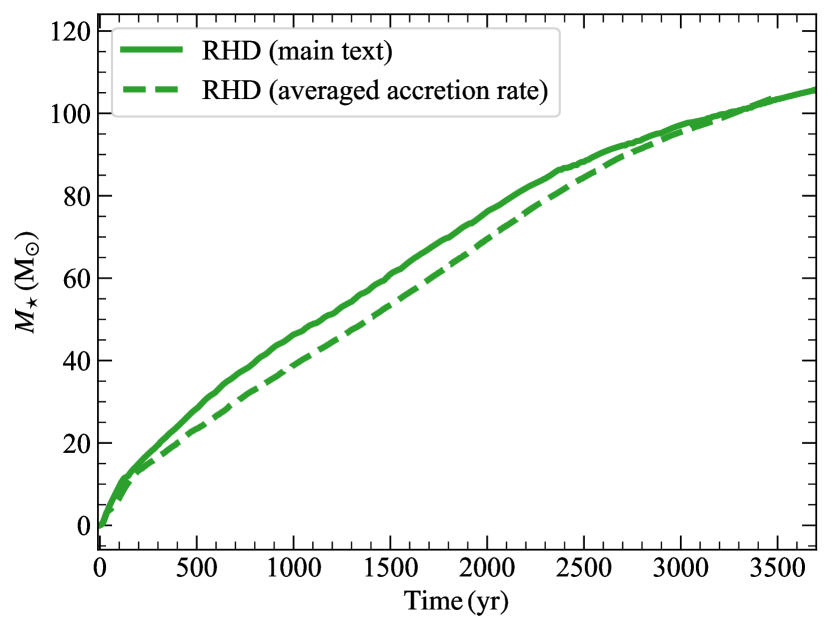
Figure 17: Mass of the central star as a function of time in the RHD case presented in the main text (solid orange curve), compared with the alternate case where instantaneous accretion rates are averaged over a $10\,\rm{yr}$ time interval to reduce numerical noise in the rate of ionizing photons.

Appendix B Saturation of the small-scale dynamo

As we mention in Section 2, we include a saturated magnetic field in our initial conditions, inspired from previous works that find very fast, exponential amplification of weak field to near saturation levels due to the small-scale dynamo (Sur et al., 2010; Schleicher et al., 2010; Turk et al., 2012; Schober et al., 2012c; Sharda et al., 2020, 2021; Sadanari et al., 2023). However, this by itself does not guarantee that the field amplification we see later on is not due to a dynamo. This is an important check because if the field gets amplified by the small-scale dynamo later on, it will also play a role in shaping the stellar mass and accretion rate, which will lead to different conclusions about how magnetic fields influence Population III star formation.

To confirm that the field remains saturated and the small-scale dynamo does not act, we calculate the strength of the turbulent component of the magnetic field, following the methodology laid out in Sharda et al. (2021). We then normalize the rms of the turbulent field, $(B_{\rm{turb}})_{\rm{rms}}$, to the gas density in order to remove contribution to field amplification from flux freezing. Figure 18 shows the resulting time evolution of this quantity. We find that this quantity only changes within a factor of few during the course of the simulation, and does not exhibit an exponential rise as expected for the small-scale dynamo (e.g., Federrath et al., 2011a; Schober et al., 2012a, 2015). Thus, the small-scale dynamo does not operate during the course of the simulation in both the MHD and RMHD runs, and the field remains close to saturation.

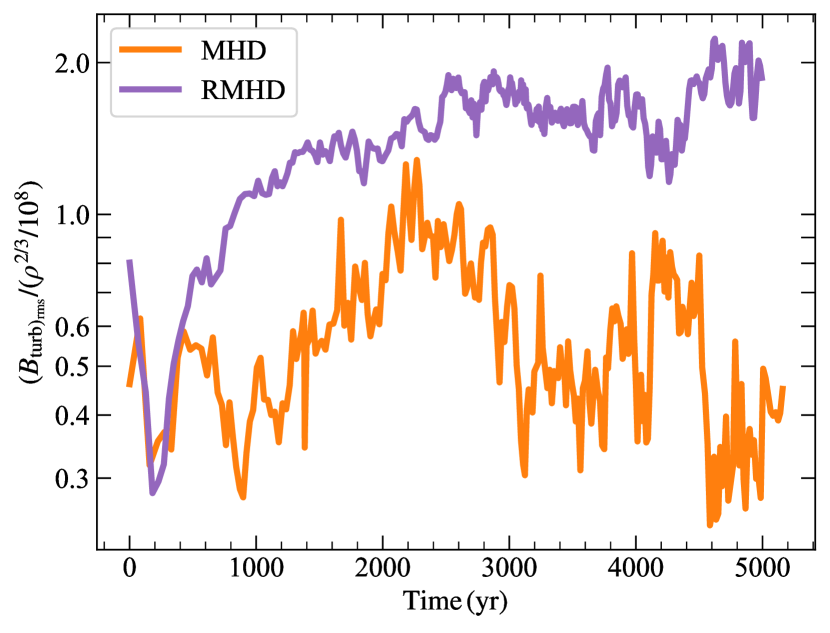
Figure 18: Quantification of the small-scale dynamo action as a function of time in the MHD and RMHD runs. The ratio on the $y$ axis denotes the rms value of the turbulent magnetic field over density to the power two-thirds (to remove the contribution of flux-freezing to field growth), and normalized by $10^{8}$. The absence of an exponential growth of the small-scale dynamo indicates that the dynamo is saturated.

Appendix C Plots for the third RMHD turbulent realization

Figure 19 and Figure 20 plots the density-weighted projections of the gas density, temperature, and mass fractions of H₂ and H⁺ for the third RMHD turbulent realization. This realization creates 7 stars by the end of the simulation, none of which are ejected from the cluster. The minimum and maximum mass of stars in the cluster is $0.7$ and $30\,\rm{M_{\odot}}$. Similar to the other two turbulent RMHD realizations, this realization also exhibits cold, molecular gas due to strong magnetic fields. However, as opposed to the second realization, this cluster remains intact and the stars are close enough that their partially ionized H ii regions overlap.

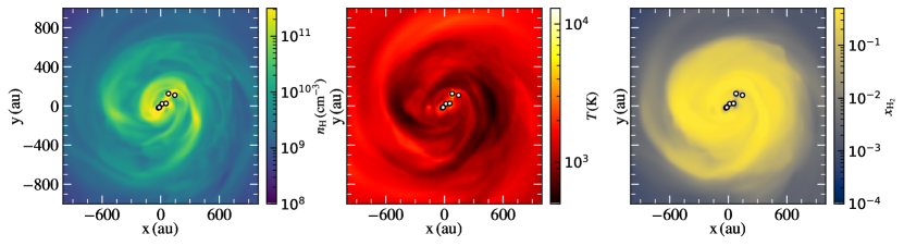
Figure 19: Density-weighted projections of the gas density, temperature and H₂ mass fraction for the third RMHD turbulent realization. This realization forms 7 stars, with masses between $0.7-30\,\rm{M_{\odot}}$.

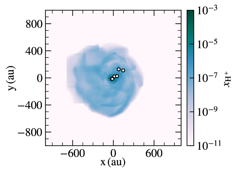
Figure 20: Same as Figure 19 but for the density-weighted projection of the mass fraction of H⁺. The cluster remains intact in this realization as opposed to the second realization, leading to overlapping partially ionized H ii regions.

References

- Abel et al. (2002) Abel T., Bryan G. L., Norman M. L., 2002, Science, 295, 93
- Aguado et al. (2022) Aguado D. S., et al., 2022, A&A, 668, A86
- Aguado et al. (2023) Aguado D. S., et al., 2023, A&A, 669, L4
- Astropy Collaboration et al. (2013) Astropy Collaboration et al., 2013, A&A, 558, A33
- Astropy Collaboration et al. (2018) Astropy Collaboration et al., 2018, AJ, 156, 123
- Astropy Collaboration et al. (2022) Astropy Collaboration et al., 2022, ApJ, 935, 167
- Baczynski et al. (2015) Baczynski C., Glover S. C. O., Klessen R. S., 2015, MNRAS, 454, 380
- Baker & Menzel (1938) Baker J. G., Menzel D. H., 1938, ApJ, 88, 52
- Balay et al. (1997) Balay S., Gropp W. D., McInnes L. C., Smith B. F., 1997, in Arge E., Bruaset A. M., Langtangen H. P., eds, Modern Software Tools in Scientific Computing. Birkhäuser Press, pp 163–202
- Bate (2009) Bate M. R., 2009, MNRAS, 392, 1363
- Bate (2012) Bate M. R., 2012, MNRAS, 419, 3115
- Borrow et al. (2023) Borrow J., Schaller M., Bahé Y. M., Schaye J., Ludlow A. D., Ploeckinger S., Nobels F. S. J., Altamura E., 2023, MNRAS, 526, 2441
- Bouchut et al. (2007) Bouchut F., Klingenberg C., Waagan K., 2007, Numerische Mathematik, 108, 7
- Bouchut et al. (2010) Bouchut F., Klingenberg C., Waagan K., 2010, Numerische Mathematik, 115, 647
- Brandenburg & Subramanian (2005) Brandenburg A., Subramanian K., 2005, Phys. Rep., 417, 1
- Bromm et al. (2002) Bromm V., Coppi P. S., Larson R. B., 2002, ApJ, 564, 23
- Bunker et al. (2023) Bunker A. J., et al., 2023, A&A, 677, A88
- Caffau et al. (2011) Caffau E., et al., 2011, Nature, 477, 67
- Chon et al. (2021) Chon S., Omukai K., Schneider R., 2021, MNRAS, 508, 4175
- Chon et al. (2023) Chon S., Hosokawa T., Omukai K., Schneider R., 2023, arXiv e-prints, p. arXiv:2312.13339
- Chung et al. (1993) Chung Y. M., Lee E. M., Masuoka T., Samson J. A. R., 1993, J. Chem. Phys., 99, 885
- Clark et al. (2011a) Clark P. C., Glover S. C. O., Smith R. J., Greif T. H., Klessen R. S., Bromm V., 2011a, Science, 331, 1040
- Clark et al. (2011b) Clark P. C., Glover S. C. O., Klessen R. S., Bromm V., 2011b, ApJ, 727, 110
- Commerçon et al. (2011) Commerçon B., Hennebelle P., Henning T., 2011, ApJ, 742, L9
- Davies et al. (2022) Davies J. J., Pontzen A., Crain R. A., 2022, MNRAS, 515, 1430
- Davies et al. (2024) Davies J. J., Pontzen A., Crain R. A., 2024, MNRAS, 527, 4705
- Díaz et al. (2024) Díaz V. B., Schleicher D. R. G., Latif M. A., Grete P., Banerjee R., 2024, A&A, 684, A195
- Donnan et al. (2023) Donnan C. T., et al., 2023, MNRAS, 518, 6011
- Drummond et al. (2020) Drummond B., et al., 2020, A&A, 636, A68
- Dubey et al. (2008) Dubey A., et al., 2008, in Pogorelov N. V., Audit E., Zank G. P., eds, Astronomical Society of the Pacific Conference Series Vol. 385, Numerical Modeling of Space Plasma Flows. p. 145
- Dubey et al. (2013) Dubey A., et al., 2013, in 2013 5th International Workshop on Software Engineering for Computational Science and Engineering (SE-CSE). pp 1–8, doi:10.1109/SECSE.2013.6615093
- Eggenberger et al. (2008) Eggenberger P., Meynet G., Maeder A., Hirschi R., Charbonnel C., Talon S., Ekström S., 2008, Ap&SS, 316, 43
- Ezzeddine et al. (2019) Ezzeddine R., et al., 2019, ApJ, 876, 97
- Federrath (2016) Federrath C., 2016, Journal of Plasma Physics, 82, 535820601
- Federrath & Klessen (2012) Federrath C., Klessen R. S., 2012, ApJ, 761, 156
- Federrath et al. (2010a) Federrath C., Roman-Duval J., Klessen R. S., Schmidt W., Mac Low M. M., 2010a, A&A, 512, A81
- Federrath et al. (2010b) Federrath C., Banerjee R., Clark P. C., Klessen R. S., 2010b, ApJ, 713, 269
- Federrath et al. (2011a) Federrath C., Chabrier G., Schober J., Banerjee R., Klessen R. S., Schleicher D. R. G., 2011a, Phys. Rev. Lett., 107, 114504
- Federrath et al. (2011b) Federrath C., Banerjee R., Seifried D., Clark P. C., Klessen R. S., 2011b, in Alves J., Elmegreen B. G., Girart J. M., Trimble V., eds, IAU Symposium Vol. 270, Computational Star Formation. pp 425–428 (arXiv:1007.2504), doi:10.1017/S1743921311000755
- Federrath et al. (2011c) Federrath C., Sur S., Schleicher D. R. G., Banerjee R., Klessen R. S., 2011c, ApJ, 731, 62
- Federrath et al. (2014) Federrath C., Schober J., Bovino S., Schleicher D. R. G., 2014, ApJ, 797, L19
- Federrath et al. (2022) Federrath C., Roman-Duval J., Klessen R. S., Schmidt W., Mac Low M. M., 2022, TG: Turbulence Generator, Astrophysics Source Code Library, record ascl:2204.001
- Ferland et al. (1998) Ferland G. J., Korista K. T., Verner D. A., Ferguson J. W., Kingdon J. B., Verner E. M., 1998, PASP, 110, 761
- Finkelstein et al. (2023) Finkelstein S. L., et al., 2023, arXiv e-prints, p. arXiv:2311.04279
- Frebel et al. (2019) Frebel A., Ji A. P., Ezzeddine R., Hansen T. T., Chiti A., Thompson I. B., Merle T., 2019, ApJ, 871, 146
- Fryxell et al. (2000) Fryxell B., et al., 2000, ApJS, 131, 273
- Galli & Palla (1998) Galli D., Palla F., 1998, A&A, 335, 403
- Galli & Palla (2013) Galli D., Palla F., 2013, ARA&A, 51, 163
- Girichidis et al. (2012) Girichidis P., Federrath C., Banerjee R., Klessen R. S., 2012, MNRAS, 420, 613
- Glover & Savin (2009) Glover S. C. O., Savin D. W., 2009, MNRAS, 393, 911
- Goodwin et al. (2004a) Goodwin S. P., Whitworth A. P., Ward-Thompson D., 2004a, A&A, 414, 633
- Goodwin et al. (2004b) Goodwin S. P., Whitworth A. P., Ward-Thompson D., 2004b, A&A, 423, 169
- Grassi et al. (2014) Grassi T., Bovino S., Schleicher D. R. G., Prieto J., Seifried D., Simoncini E., Gianturco F. A., 2014, MNRAS, 439, 2386
- Greif et al. (2012) Greif T. H., Bromm V., Clark P. C., Glover S. C. O., Smith R. J., Klessen R. S., Yoshida N., Springel V., 2012, MNRAS, 424, 399
- Grudić et al. (2022) Grudić M. Y., Guszejnov D., Offner S. S. R., Rosen A. L., Raju A. N., Faucher-Giguère C.-A., Hopkins P. F., 2022, MNRAS, 512, 216
- Guszejnov et al. (2016) Guszejnov D., Krumholz M. R., Hopkins P. F., 2016, MNRAS, 458, 673
- Haemmerlé et al. (2013) Haemmerlé L., Eggenberger P., Meynet G., Maeder A., Charbonnel C., 2013, A&A, 557, A112
- Haemmerlé et al. (2016) Haemmerlé L., Eggenberger P., Meynet G., Maeder A., Charbonnel C., 2016, A&A, 585, A65
- Haemmerlé et al. (2018) Haemmerlé L., Woods T. E., Klessen R. S., Heger A., Whalen D. J., 2018, MNRAS, 474, 2757
- Harikane et al. (2023) Harikane Y., et al., 2023, ApJS, 265, 5
- Harris et al. (2020) Harris C. R., et al., 2020, Nature, 585, 357
- Haugen et al. (2004) Haugen N. E., Brandenburg A., Dobler W., 2004, Phys. Rev. E, 70, 016308
- He & Ricotti (2023) He C.-C., Ricotti M., 2023, MNRAS, 522, 5374
- Heger & Woosley (2002) Heger A., Woosley S. E., 2002, ApJ, 567, 532
- Heger & Woosley (2010) Heger A., Woosley S. E., 2010, ApJ, 724, 341
- Hennebelle & Grudić (2024) Hennebelle P., Grudić M. Y., 2024, arXiv e-prints, p. arXiv:2404.07301
- Hirano & Bromm (2018) Hirano S., Bromm V., 2018, MNRAS, 476, 3964
- Hirano & Machida (2022) Hirano S., Machida M. N., 2022, ApJ, 935, L16
- Hirano et al. (2014) Hirano S., Hosokawa T., Yoshida N., Umeda H., Omukai K., Chiaki G., Yorke H. W., 2014, ApJ, 781, 60
- Hosokawa & Omukai (2009) Hosokawa T., Omukai K., 2009, ApJ, 691, 823
- Hosokawa et al. (2010) Hosokawa T., Yorke H. W., Omukai K., 2010, ApJ, 721, 478
- Hosokawa et al. (2011) Hosokawa T., Omukai K., Yoshida N., Yorke H. W., 2011, Science, 334, 1250
- Hosokawa et al. (2013) Hosokawa T., Yorke H. W., Inayoshi K., Omukai K., Yoshida N., 2013, ApJ, 778, 178
- Hosokawa et al. (2016) Hosokawa T., Hirano S., Kuiper R., Yorke H. W., Omukai K., Yoshida N., 2016, ApJ, 824, 119
- Hui & Gnedin (1997) Hui L., Gnedin N. Y., 1997, MNRAS, 292, 27
- Hunter (2007) Hunter J. D., 2007, Computing in Science & Engineering, 9, 90
- Inayoshi et al. (2020) Inayoshi K., Visbal E., Haiman Z., 2020, ARA&A, 58, 27
- Ishigaki et al. (2018) Ishigaki M. N., Tominaga N., Kobayashi C., Nomoto K., 2018, ApJ, 857, 46
- Jappsen & Klessen (2004) Jappsen A. K., Klessen R. S., 2004, A&A, 423, 1
- Jaura et al. (2022) Jaura O., Glover S. C. O., Wollenberg K. M. J., Klessen R. S., Geen S., Haemmerlé L., 2022, MNRAS, 512, 116
- Jeena et al. (2023) Jeena S. K., Banerjee P., Chiaki G., Heger A., 2023, MNRAS, 526, 4467
- Ji et al. (2024) Ji A. P., et al., 2024, arXiv e-prints, p. arXiv:2401.02484
- Johnson (2015) Johnson J. L., 2015, MNRAS, 453, 2771
- Katz (2022) Katz H., 2022, MNRAS, 512, 348
- Kewley et al. (2019) Kewley L. J., Nicholls D. C., Sutherland R. S., 2019, ARA&A, 57, 511
- Kim et al. (2023) Kim J.-G., Gong M., Kim C.-G., Ostriker E. C., 2023, ApJS, 264, 10
- Klessen & Glover (2023) Klessen R. S., Glover S. C. O., 2023, ARA&A, 61, 65
- Krumholz (2011) Krumholz M. R., 2011, ApJ, 743, 110
- Krumholz & Federrath (2019) Krumholz M. R., Federrath C., 2019, Frontiers in Astronomy and Space Sciences, 6, 7
- Krumholz et al. (2012) Krumholz M. R., Klein R. I., McKee C. F., 2012, ApJ, 754, 71
- Krumholz et al. (2016) Krumholz M. R., Myers A. T., Klein R. I., McKee C. F., 2016, MNRAS, 460, 3272
- Kudritzki (2002) Kudritzki R. P., 2002, ApJ, 577, 389
- Kuiper et al. (2016) Kuiper R., Turner N. J., Yorke H. W., 2016, ApJ, 832, 40
- Kulkarni et al. (2021) Kulkarni M., Visbal E., Bryan G. L., 2021, ApJ, 917, 40
- Larkin et al. (2023) Larkin M. M., Gerasimov R., Burgasser A. J., 2023, AJ, 165, 2
- Latif et al. (2013) Latif M. A., Schleicher D. R. G., Schmidt W., Niemeyer J., 2013, MNRAS, 432, 668
- Latif et al. (2014) Latif M. A., Schleicher D. R. G., Schmidt W., 2014, MNRAS, 440, 1551
- Latif et al. (2018) Latif M. A., Volonteri M., Wise J. H., 2018, MNRAS, 476, 5016
- Liao et al. (2019) Liao W.-T., Turk M., Schive H.-Y., 2019, arXiv e-prints, p. arXiv:1911.07898
- Lin et al. (2011) Lin M.-K., Krumholz M. R., Kratter K. M., 2011, MNRAS, 416, 580
- Liu & Bromm (2018) Liu B., Bromm V., 2018, MNRAS, 476, 1826
- Liu & Bromm (2020) Liu B., Bromm V., 2020, MNRAS, 497, 2839
- Liu & Shemansky (2012) Liu X., Shemansky D. E., 2012, Journal of Physics B Atomic Molecular Physics, 45, 095203
- Machida & Doi (2013) Machida M. N., Doi K., 2013, MNRAS, 435, 3283
- Machida et al. (2006) Machida M. N., Omukai K., Matsumoto T., Inutsuka S.-i., 2006, ApJ, 647, L1
- Machida et al. (2008) Machida M. N., Matsumoto T., Inutsuka S.-i., 2008, ApJ, 685, 690
- Maiolino et al. (2023) Maiolino R., et al., 2023, arXiv e-prints, p. arXiv:2306.00953
- Mardini et al. (2022) Mardini M. K., et al., 2022, MNRAS, 517, 3993
- Marigo et al. (2001) Marigo P., Girardi L., Chiosi C., Wood P. R., 2001, A&A, 371, 152
- Mathew & Federrath (2021) Mathew S. S., Federrath C., 2021, MNRAS, 507, 2448
- McKee et al. (2020) McKee C. F., Stacy A., Li P. S., 2020, MNRAS, 496, 5528
- Mebane et al. (2018) Mebane R. H., Mirocha J., Furlanetto S. R., 2018, MNRAS, 479, 4544
- Menon & Sharda (2024) Menon S. H., Sharda P., 2024, MNRAS, in prep.
- Menon et al. (2020) Menon S. H., Federrath C., Kuiper R., 2020, MNRAS, 493, 4643
- Menon et al. (2021) Menon S. H., Federrath C., Klaassen P., Kuiper R., Reiter M., 2021, MNRAS, 500, 1721
- Menon et al. (2022) Menon S. H., Federrath C., Krumholz M. R., Kuiper R., Wibking B. D., Jung M., 2022, MNRAS, 512, 401
- Murphy et al. (2021) Murphy L. J., Groh J. H., Farrell E., Meynet G., Ekström S., Tsiatsiou S., Hackett A., Martinet S., 2021, MNRAS, 506, 5731
- Nakauchi et al. (2019) Nakauchi D., Omukai K., Susa H., 2019, MNRAS, 488, 1846
- Nandal et al. (2024) Nandal D., Sibony Y., Tsiatsiou S., 2024, arXiv e-prints, p. arXiv:2405.11235
- Nickerson et al. (2018) Nickerson S., Teyssier R., Rosdahl J., 2018, MNRAS, 479, 3206
- Nordlander et al. (2019) Nordlander T., et al., 2019, MNRAS, 488, L109
- Oliphant (2006) Oliphant T. E., 2006, A guide to NumPy. Vol. 1, Trelgol Publishing USA
- Omukai & Nishi (1998) Omukai K., Nishi R., 1998, ApJ, 508, 141
- Omukai & Palla (2001) Omukai K., Palla F., 2001, ApJ, 561, L55
- Omukai & Palla (2003) Omukai K., Palla F., 2003, ApJ, 589, 677
- Omukai et al. (2005) Omukai K., Tsuribe T., Schneider R., Ferrara A., 2005, ApJ, 626, 627
- Osterbrock (1989) Osterbrock D. E., 1989, Astrophysics of gaseous nebulae and active galactic nuclei
- Peters et al. (2010) Peters T., Klessen R. S., Mac Low M.-M., Banerjee R., 2010, ApJ, 725, 134
- Prole et al. (2022a) Prole L. R., Clark P. C., Klessen R. S., Glover S. C. O., 2022a, MNRAS, 510, 4019
- Prole et al. (2022b) Prole L. R., Clark P. C., Klessen R. S., Glover S. C. O., Pakmor R., 2022b, MNRAS, 516, 2223
- Prole et al. (2023) Prole L. R., Clark P. C., Priestley F. D., Glover S. C. O., Regan J. A., 2023, arXiv e-prints, p. arXiv:2310.10730
- Prole et al. (2024) Prole L. R., Regan J. A., Glover S. C. O., Klessen R. S., Priestley F. D., Clark P. C., 2024, A&A, 685, A31
- Pudritz (1981a) Pudritz R. E., 1981a, MNRAS, 195, 881
- Pudritz (1981b) Pudritz R. E., 1981b, MNRAS, 195, 897
- Riaz et al. (2018) Riaz R., Bovino S., Vanaverbeke S., Schleicher D. R. G., 2018, MNRAS, 479, 667
- Riaz et al. (2023) Riaz R., Schleicher D. R. G., Bovino S., Vanaverbeke S., Klessen R. S., 2023, MNRAS, 518, 4895
- Roberti et al. (2024) Roberti L., Limongi M., Chieffi A., 2024, ApJS, 270, 28
- Rosen & Krumholz (2020) Rosen A. L., Krumholz M. R., 2020, AJ, 160, 78
- Saad et al. (2022) Saad C. R., Bromm V., El Eid M., 2022, MNRAS, 516, 3130
- Sadanari et al. (2021) Sadanari K. E., Omukai K., Sugimura K., Matsumoto T., Tomida K., 2021, MNRAS, 505, 4197
- Sadanari et al. (2023) Sadanari K. E., Omukai K., Sugimura K., Matsumoto T., Tomida K., 2023, MNRAS, 519, 3076
- Schleicher et al. (2010) Schleicher D. R. G., Banerjee R., Sur S., Arshakian T. G., Klessen R. S., Beck R., Spaans M., 2010, A&A, 522, A115
- Schober et al. (2012a) Schober J., Schleicher D., Federrath C., Klessen R., Banerjee R., 2012a, Phys. Rev. E, 85, 026303
- Schober et al. (2012b) Schober J., Schleicher D., Bovino S., Klessen R. S., 2012b, Phys. Rev. E, 86, 066412
- Schober et al. (2012c) Schober J., Schleicher D., Federrath C., Glover S., Klessen R. S., Banerjee R., 2012c, ApJ, 754, 99
- Schober et al. (2015) Schober J., Schleicher D. R. G., Federrath C., Bovino S., Klessen R. S., 2015, Phys. Rev. E, 92, 023010
- Sharda & Krumholz (2022) Sharda P., Krumholz M. R., 2022, MNRAS, 509, 1959
- Sharda et al. (2019) Sharda P., Krumholz M. R., Federrath C., 2019, MNRAS, 490, 513
- Sharda et al. (2020) Sharda P., Federrath C., Krumholz M. R., 2020, MNRAS, 497, 336
- Sharda et al. (2021) Sharda P., Federrath C., Krumholz M. R., Schleicher D. R. G., 2021, MNRAS, 503, 2014
- Sharda et al. (2023) Sharda P., Amarsi A. M., Grasha K., Krumholz M. R., Yong D., Chiaki G., Roy A., Nordlander T., 2023, MNRAS, 518, 3985
- Sharda et al. (2024) Sharda P., Wibking B. D., Zingale M., Krumholz M. R., Katz M., Zhang W., Kriel N., Vijayan A., 2024, MNRAS, in prep.
- Skúladóttir et al. (2021) Skúladóttir Á., et al., 2021, ApJ, 915, L30
- Skúladóttir et al. (2024) Skúladóttir Á., Koutsouridou I., Vanni I., Amarsi A. M., Lucchesi R., Salvadori S., Aguado D., 2024, arXiv e-prints, p. arXiv:2404.19086
- Stacy & Bromm (2014) Stacy A., Bromm V., 2014, ApJ, 785, 73
- Stacy et al. (2011) Stacy A., Bromm V., Loeb A., 2011, MNRAS, 413, 543
- Stacy et al. (2012) Stacy A., Greif T. H., Bromm V., 2012, MNRAS, 422, 290
- Stacy et al. (2016) Stacy A., Bromm V., Lee A. T., 2016, MNRAS, 462, 1307
- Stacy et al. (2022) Stacy A., McKee C. F., Lee A. T., Klein R. I., Li P. S., 2022, MNRAS, 511, 5042
- Stahler et al. (1986) Stahler S. W., Palla F., Salpeter E. E., 1986, ApJ, 302, 590
- Strömgren (1939) Strömgren B., 1939, ApJ, 89, 526
- Subramanian (2019) Subramanian K., 2019, Galaxies, 7, 47
- Sugimura et al. (2020) Sugimura K., Matsumoto T., Hosokawa T., Hirano S., Omukai K., 2020, ApJ, 892, L14
- Sugimura et al. (2023) Sugimura K., Matsumoto T., Hosokawa T., Hirano S., Omukai K., 2023, ApJ, 959, 17
- Sur et al. (2010) Sur S., Schleicher D. R. G., Banerjee R., Federrath C., Klessen R. S., 2010, ApJ, 721, L134
- Sur et al. (2012) Sur S., Federrath C., Schleicher D. R. G., Banerjee R., Klessen R. S., 2012, MNRAS, 423, 3148
- Susa et al. (2014) Susa H., Hasegawa K., Tominaga N., 2014, ApJ, 792, 32
- Truelove et al. (1997) Truelove J. K., Klein R. I., McKee C. F., Holliman John H. I., Howell L. H., Greenough J. A., 1997, ApJ, 489, L179
- Tsiatsiou et al. (2024) Tsiatsiou S., et al., 2024, arXiv e-prints, p. arXiv:2404.16512
- Turk et al. (2011) Turk M. J., Smith B. D., Oishi J. S., Skory S., Skillman S. W., Abel T., Norman M. L., 2011, ApJS, 192, 9
- Turk et al. (2012) Turk M. J., Oishi J. S., Abel T., Bryan G. L., 2012, ApJ, 745, 154
- Umeda et al. (2016) Umeda H., Hosokawa T., Omukai K., Yoshida N., 2016, ApJ, 830, L34
- Van der Velden (2020) Van der Velden E., 2020, The Journal of Open Source Software, 5, 2004
- Venditti et al. (2023) Venditti A., Graziani L., Schneider R., Pentericci L., Di Cesare C., Maio U., Omukai K., 2023, MNRAS, 522, 3809
- Vink et al. (2001) Vink J. S., de Koter A., Lamers H. J. G. L. M., 2001, A&A, 369, 574
- Virtanen et al. (2020) Virtanen P., et al., 2020, Nature Methods, 17, 261
- Volpato et al. (2024) Volpato G., Marigo P., Costa G., Bressan A., Trabucchi M., Girardi L., Addari F., 2024, ApJ, 961, 89
- Waagan (2009) Waagan K., 2009, Journal of Computational Physics, 228, 8609
- Waagan et al. (2011) Waagan K., Federrath C., Klingenberg C., 2011, Journal of Computational Physics, 230, 3331
- Wang et al. (2012) Wang F. Y., Bromm V., Greif T. H., Stacy A., Dai Z. G., Loeb A., Cheng K. S., 2012, ApJ, 760, 27
- Wibking & Krumholz (2022) Wibking B. D., Krumholz M. R., 2022, MNRAS, 512, 1430
- Wolcott-Green et al. (2011) Wolcott-Green J., Haiman Z., Bryan G. L., 2011, MNRAS, 418, 838
- Wollenberg et al. (2020) Wollenberg K. M. J., Glover S. C. O., Clark P. C., Klessen R. S., 2020, MNRAS, 494, 1871
- Woods et al. (2019) Woods T. E., et al., 2019, Publ. Astron. Soc. Australia, 36, e027
- Wünsch et al. (2018) Wünsch R., Walch S., Dinnbier F., Whitworth A., 2018, MNRAS, 475, 3393
- Wurster & Li (2018) Wurster J., Li Z.-Y., 2018, Frontiers in Astronomy and Space Sciences, 5, 39
- Yajima et al. (2023) Yajima H., Abe M., Fukushima H., Ono Y., Harikane Y., Ouchi M., Hashimoto T., Khochfar S., 2023, MNRAS, 525, 4832
- Yoon et al. (2012) Yoon S. C., Dierks A., Langer N., 2012, A&A, 542, A113
- Zhang et al. (2022) Zhang J., et al., 2022, IEEE Transactions on Parallel and Distributed Systems, 33, 842