Truthful Dataset Valuation by Pointwise Mutual Information

Abstract

A common way to evaluate a dataset in ML involves training a model on this dataset and assessing the model’s performance on a test set. However, this approach has two issues: (1) it may incentivize undesirable data manipulation in data marketplaces, as the self-interested data providers seek to modify the dataset to maximize their evaluation scores; (2) it may select datasets that overfit to potentially small test sets. We propose a new data valuation method that provably guarantees the following: data providers always maximize their expected score by truthfully reporting their observed data. Any manipulation of the data, including but not limited to data duplication, adding random data, data removal, or re-weighting data from different groups, cannot increase their expected score. Our method, following the paradigm of proper scoring rules, measures the pointwise mutual information (PMI) of the test dataset and the evaluated dataset. However, computing the PMI of two datasets is challenging. We introduce a novel PMI measuring method that greatly improves tractability within Bayesian machine learning contexts. This is accomplished through a new characterization of PMI that relies solely on the posterior probabilities of the model parameter at an arbitrarily selected value. Finally, we support our theoretical results with simulations and further test the effectiveness of our data valuation method in identifying the top datasets among multiple data providers. Interestingly, our method outperforms the standard approach of selecting datasets based on trained model’s test performance, suggesting that our truthful valuation score can also be more robust to overfitting.

1 Introduction

In the age of artificial intelligence (AI), data serves as the lifeblood that fuels innovation and development. The intricate models powering AI systems heavily rely on vast and diverse datasets to learn, adapt, and make informed decisions. Essentially, the quality and makeup of the datasets used for training and testing directly shape the reliability and adaptability of AI systems.

The success of AI models undeniably relies on the huge volume of publicly-available data on the web. However, owing to challenges related to data quality and the demands for task-specific datasets, machine learning developers increasingly aggregate and purchase data from different providers. This has led to the emergence of a rapidly growing market of data providers, data sellers, and data collectors. For example, Amazon Data Exchange is a platform whereby third parties vendors can sell and buy thousands of datasets. In addition, various platforms offer data labeling services tailored to diverse tasks, such as Amazon Mechanical Turk and Toloka AI.

A central challenge for this data marketplace lies in developing a methodology for data evaluation. The data buyers are tasked with evaluating datasets in the market to inform their procurement decisions; data labeling platforms must assess the data produced by workers for quality assurance. The most common approaches to evaluate a dataset involves training a model with the dataset and then testing how well a model performs on a test set. However, this type of evaluation approach may give rise to two issues: (1) it might incentivize undesirable data manipulation when deployed in the data marketplace, as the evaluated data providers, being human, are inherently self-interested and seek to maximize their evaluation scores; (2) it may endorse datasets that overfit to the test set, which could potentially be a small dataset.

Consider the following example. Suppose we want to collect data for the binary classification of examples $(x,y)$, where instances $x\in\mathbb{R}$ and $y\in\{+1,-1\}$. Assume that instances with label $+1$ are drawn independently from the Gaussian distribution $\mathcal{N}(1,1)$ and the instances with label $-1$ are drawn independently from $\mathcal{N}(-1,1)$. Suppose we have a test dataset that can be used for data evaluation and the test dataset consists of $50\%$ positive instances (with label $+1$) and $50\%$ negative instances (with label $-1$), and this percentage is publicly shared. Consider a data provider who observes much more positive instances than negative instances in their dataset. If we evaluate a dataset by training a model on the dataset and evaluating its test error (the dataset receives a higher score for a smaller test error), the data provider may want to discard some positive data points under the belief that this will make the dataset more aligned with the test data and thus improve the test error.

A data collector certainly do not want such data manipulation: the collector may have many different applications, including future ones that remain unknown. Therefore, they may not want the provider to manipulate the data to overfit to a particular and potentially small test set. In general, Goodhart’s law states that when a measure becomes a target, it ceases to be a good measure. A data valuation measure that is not incentive compatible is more likely to be a target for self-interested providers and hence may not be good. Moreover, such manipulation may lead to the disposal of less observed data from the tail of the distribution. However, the less common data can be more valuable for developing reliable machine learning than the more frequent data from the mode.

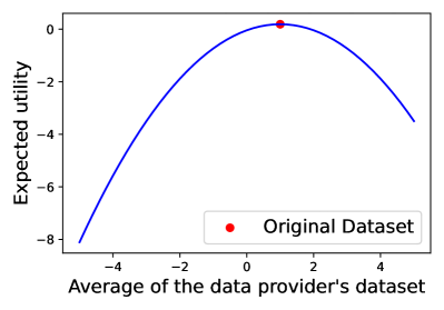
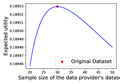
Figure 1: A data provider’s expected PMI score (which we will introduce in Sec. 3) when (1) shifting the mean of the whole dataset without changing its size, (2) changing the dataset size without changing the mean. The expected score is maximized at truthfully reporting the original dataset.

Our contributions.

To prevent this type of strategic overfitting, we propose a data valuation method, termed the PMI dataset score, that guarantees the following: after the data provider sees their dataset, the expected score that they will receive is always maximized by truthfully reporting the observed dataset. Any form of data manipulation cannot increase their expected score, including but not limited to data duplication, adding random data, data removal, and re-weighting data from different groups. In Figure 1, we demonstrate a data provider’s expected score when we collect data to estimate the mean of the population distribution (in the presence of possible distributional shifts in the test data). We illustrate two types of data manipulation: (1) shift the mean of the whole dataset without changing its size, and (2) change the dataset size by duplication or adding random data without changing the mean. As shown in the plots, these data manipulations will only decrease the expected score. The details are provided in Section 4.1.

Following the paradigm of proper scoring rules (see Section 2.1), we achieve this type of truthfulness guarantee by measuring the pointwise mutual information (PMI) of the test dataset and the evaluated dataset, which represents how much seeing a dataset increases the log-likelihood of seeing the test data. However, computing PMI of two datasets is highly non-trivial (see Section 2.1). Our PMI dataset score provides a novel PMI measuring method that significantly improves tractability in Bayesian machine learning contexts. This is achieved through a characterization of PMI that only requires the posterior probabilities of the model parameter at an arbitrarily-picked value $\eta$: after seeing the data, what is the probability that the true model parameter equals $\eta$? This simplified PMI expression also enables new interpretations of PMI between datasets. For Gaussian models, the PMI between two datasets essentially captures two aspects: (1) it measures the similarity between the test dataset and the evaluated dataset; (2) it measures how much the two datasets enhance our confidence in estimating the model parameter. Finally, we evaluate the computational efficiency of the PMI dataset score and demonstrate through simulations that it discourages data manipulation and is more robust to overfitting than selecting datasets based on test scores.

1.1 Related works

Data Valuation.

The assessment of data value has been actively studied in the data valuation literature. A standard approach is to measure the change in the test accuracy after removing a single training data point of interest. Data Shapley by Ghorbani and Zou (2019) deploys the Shapley value from cooperative game theory to ML settings, and several variants that improve its computational efficiency or relax underlying conditions have been proposed (Jia et al., 2019; Kwon and Zou, 2021; Wang and Jia, 2022). An alternative common approach utilizes the influence function introduced in robust statistics (Koh and Liang, 2017; Feldman and Zhang, 2020). This method provides a mathematically rigorous interpretation of data values and has been implemented in various applications, such as image classification and sentiment analysis, or text-to-image generation (Park et al., 2023; Kwon et al., 2023). We refer the readers to Jiang et al. (2023) for a comprehensive review.

Data valuation algorithms have demonstrated promising results in many downstream ML tasks, including the identification of low-quality data points and the attribution of model predictions to the most relevant training data points (Jiang et al., 2023). However, most of the developed algorithms focus on evaluating individual data points, and the impact of data modification on value estimation has not been studied much. The main goal of this work is to develop an evaluation method for the entire dataset that can prevent a data provider from modifying the dataset.

Peer prediction approach.

Our method adopts tools from the literature of peer prediction Miller et al. (2005); Prelec (2004); Jurca and Faltings (2008); Radanovic and Faltings (2013, 2014); Witkowski and Parkes (2012); Kong and Schoenebeck (2018a); Schoenebeck and Yu (2020), a subfield in economics that studies eliciting truthful information without ground truth. Among the extensive literature, Kong and Schoenebeck (2018b); Chen et al. (2020) are most relevant to our work. Kong and Schoenebeck (2018b) proposed a pointwise mutual information based peer prediction method that collects two agents’ predictions about a latent label. This method was later introduced to data valuation by Chen et al. (2020) where they studied strictly truthful methods, and considered exponential family distributions. However, their computation of the pointwise mutual information is much more complex than ours: they compute the pointwise mutual information by a complex integral of the product of two posteriors divided by the prior, whereas ours only uses posterior probabilities at one point. As a result, our score is much easier to compute or estimate in general.

2 Model

A data collector wants to gather data for some statistical estimation or machine learning task with a model parameterized by ${\bm{\theta}}\in\Theta\subseteq\mathbb{R}^{k}$, which is drawn from a prior distribution $p({\bm{\theta}})$. The data analyst holds a test dataset $T$ that consists of $N_{T}$ i.i.d. data points $({\mathbf{x}}_{T}^{(1)},y_{T}^{(1)})$, $\dots$, $({\mathbf{x}}_{T}^{(N_{T})},y_{T}^{(N_{T})})$ drawn from $p({\mathbf{x}}_{T},y_{T}|{\bm{\theta}})$. There is a data provider who holds a dataset $D$ that contains $N_{D}$ i.i.d. data points $({\mathbf{x}}_{D}^{(1)},y_{D}^{(1)}),\dots,({\mathbf{x}}_{D}^{(N_{D})},y_{D}^{(N_{D})})$ drawn from $p({\mathbf{x}}_{D},y_{D}|{\bm{\theta}})$. The two datasets do not have to follow the same distribution, so $p({\mathbf{x}}_{D},y_{D}|{\bm{\theta}})$ can be different from $p({\mathbf{x}}_{T},y_{T}|{\bm{\theta}})$. We assume that $D$ and $T$ are independent conditioning on ${\bm{\theta}}$, i.e.,

$$p(D,T|{\bm{\theta}})=p(D|{\bm{\theta}})p(T|{\bm{\theta}}).$$

We denote the support of $D$ and $T$ by $\mathcal{D}$ and $\mathcal{T}$ respectively.

We consider the data collector’s problem of data valuation. The data collector needs to decide a rule for evaluating the data, which can be represented as a function $U:\mathcal{D}\times\mathcal{T}\to\mathbb{R}$ that takes in the evaluated dataset $d\in\mathcal{D}$ and the test dataset $t\in\mathcal{T}$ and outputs a real number $U(d,t)$ that represents the score of the evaluated dataset $d$. The data collector will post and commit to the rule, and the data provider will respond to the rule strategically in order to maximize their own scores. So the timeline is as follows.

1. The data collector posts a data valuation metric $U(d,t)$ for $d\in\mathcal{D},t\in\mathcal{T}$.

2. Nature draws ${\bm{\theta}}\sim p({\bm{\theta}})$ and the data collector draws a test dataset $T\sim p(T|{\bm{\theta}})$ and the data provider observes a dataset $D\sim p(D|{\bm{\theta}})$.

3. After seeing the metric $U(\cdot)$ and the dataset $D$, the data provider chooses a dataset $D^{\prime}$ and submits it to the data collector.

4. The data collector uses the posted metric to evaluate the submitted dataset, so the data provider receives a score of $U(D^{\prime},T)$.

We consider self-interested data providers whose goal is to maximize their own expected score $\mathbb{E}[U(D^{\prime},T)|D]$. If the metric $U(\cdot)$ is not carefully designed, a data provider may get a higher score in expectation by manipulating their data (choosing $D^{\prime}\neq D$), when they have knowledge about the distribution of the test data. To forestall such unwanted data manipulation, we want to assure that, assuming the data provider possesses maximal knowledge: they know the underlying distributions $p({\bm{\theta}})$, $p(T|{\bm{\theta}})$, and $p(D|{\bm{\theta}})$, it is impossible for them to increase their expected score through any form of data manipulation. To formalize this goal, we first define knowledgeable data providers.

Definition 2.1 (Knowledgeable data providers).

A knowledgeable data provider knows the underlying distributions $p({\bm{\theta}}),p(T|{\bm{\theta}})$, and $p(D|{\bm{\theta}})$. After observing $D$, their belief about the test dataset becomes $p(T|D)=\int_{\bm{\theta}}p(T|{\bm{\theta}})p({\bm{\theta}}|D)\,d{\bm{\theta}}$. Based on this posterior belief, they assess their expected score when reporting a dataset $D^{\prime}$.

In practice, a data provider may not have precise knowledge of the distributions, but assuming such knowledge only makes our results stronger. In contrast, for the data collector, we do not want to assume a lot of prior knowledge when she designs the valuation metric. But designing a desirable metric is challenging; without any prior knowledge about the underlying distribution, it can be intractable. So we assume that the data collector has some basic knowledge about the underlying distributions; more specifically, we assume that the underlying distribution $p({\bm{\theta}},D,T)$ is specified by a standard Bayesian machine learning model.

Assumption 2.2.

The underlying distribution $p({\bm{\theta}},D,T)$ is specified by a standard Bayesian machine learning model. The data collector knows $p({\bm{\theta}})$ and is able to compute/estimate the posterior of the parameter $p({\bm{\theta}}=\eta|\text{a dataset})$ at a specific point $\eta$ given any dataset.

Then the data collector’s goal is to design a valuation metric that guarantees truthfulness for any possible data distributions $p(D|{\bm{\theta}})$ and $p(T|{\bm{\theta}})$, given a prior $p({\bm{\theta}})$.

Definition 2.3 (Truthfulness).

Given the prior $p({\bm{\theta}})$, a data valuation metric $U:\mathcal{D}\times\mathcal{T}\to\mathbb{R}$ is truthful if a knowledgeable data provider’s expected score conditional on her observed data $D=d$ is maximized by truthfully providing the observed dataset $d$, for any possible realization of the evaluated dataset $d\in\mathcal{D}$ and any possible underlying distribution. Formally, for any distributions $p(D|{\bm{\theta}}),p(T|{\bm{\theta}})$, and any observed dataset $d\in\mathcal{D}$ and any $d^{\prime}\neq d\in\mathcal{D}$,

$$\mathbb{E}_{T}[U(d^{\prime},T)|D=d]\leq\mathbb{E}_{T}[U(d,T)|D=d],$$

where the expectation is taken over $T\sim p(T|D=d)=\int_{\bm{\theta}}p(T|{\bm{\theta}})p({\bm{\theta}}|D=d)\,d{\bm{\theta}}$.

We want to emphasize the following regarding our model.

Remark 2.4.

In this definition, we assume that a data provider’s identity can be verified, and each data provider is only allowed to submit one dataset.

Remark 2.5.

In the definition it may seem that the data providers need to know the underlying distributions in order to assess their expected scores. But since our definition requires a metric to be truthful for any possible underlying distribution, the data providers will be incentivized to report truthfully even if they are uncertain about the distributions, since truthful reporting is always optimal.

Remark 2.6.

We assume that all of the data provider’s observations about ${\bm{\theta}}$ are included in the dataset $D$. If the data provider observes other information about ${\bm{\theta}}$ that is not reported to the data collector, then in general, it is impossible to design meaningful truthful data valuation functions. See the proof in Section B.2.

Remark 2.7.

We assume the data provider is uncertain about ${\bm{\theta}}$, and the provider evaluates the expected score based on the posterior belief $p({\bm{\theta}}|D=d)$ before receiving the final score or seeing the trained model (i.e., the truthfulness is guaranteed interim). This does not ensure that after seeing her final score or the trained model, the data provider will not regret providing true data (truthfulness is not guaranteed ex post). One might wonder if we can ensure that the data providers will not regret. However, as proved in Section B.1, there exists no such valuation function that is non-constant.

2.1 Preliminaries

In this work, we mainly investigate the design of truthful data valuation method when the underlying distribution $p({\bm{\theta}},D,T)$ is specified by standard Bayesian machine learning models. Before introducing our method, we review existing approaches and show their limitations.

2.1.1 Scoring rules for Bayesian machine learning

First of all, if we have a generative model where the posterior predictive distribution $p(T|D)=\int_{\bm{\theta}}p(T|{\bm{\theta}})p({\bm{\theta}}|D)\,d{\bm{\theta}}$ can be efficiently computed, then truthfulness can be easily achieved by proper scoring rules Gneiting and Raftery (2007), for example, the logarithmic scoring rule Good (1952).

Proposition 2.8.

The logarithmic scoring rule $U(d,t)$ $=$ $\log p(T=t|D=d)=\log\int_{\bm{\theta}}p(T=t|{\bm{\theta}})p({\bm{\theta}}|D=d)\,d{\bm{\theta}}$ is truthful, if can be computed.

However, most of the common machine learning models do not have efficiently computable $\int_{\bm{\theta}}p(T|{\bm{\theta}})p({\bm{\theta}}|D)\,d{\bm{\theta}}$. For discriminative models, the distribution $p(T|{\bm{\theta}})$ is even not fully specified: discriminative models only make modeling assumptions on $p(y|{\mathbf{x}},{\bm{\theta}})$ but not $p({\mathbf{x}}|{\bm{\theta}})$, e.g., the Bayesian linear regression model discussed in the next section.

2.1.2 Integral PMI score

A variant of the logarithmic scoring rule is the pointwise mutual information, which is equivalent to the logarithmic scoring rule minus a constant.

Proposition 2.9.

The pointwise mutual information of $d$ and $t$, $PMI(d,t)=\log\frac{p(T=t|D=d)}{p(T=t)}$ is truthful, if can be computed.

The straightforward definition of pointwise mutual information does not simplify the task; in fact, computing the marginal data distribution $p(T=t)$ is recognized as challenging. Kong and Schoenebeck (2018b) proposes a method to compute the PMI, which only requires the posteriors and the prior of the model parameter ${\bm{\theta}}$, bypassing the need for explicit data distributions $p(T=t|D=d),p(T=t)$.

Theorem 2.10 (Integral PMI score (Kong and Schoenebeck, 2018b)).

The pointwise mutual information $PMI(d,t)=\log\int_{\bm{\theta}}p({\bm{\theta}}|D=d)p({\bm{\theta}}|T=t)/p({\bm{\theta}})\,d{\bm{\theta}}.$ Therefore the data valuation function $U(d,t)=\log\int_{\bm{\theta}}p({\bm{\theta}}|D=d)p({\bm{\theta}}|T=t)/p({\bm{\theta}})\,d{\bm{\theta}}$ is truthful.

One advantage of this integral representation is that it can (possibly) be used for discriminative models, as it only requires the prior and the posteriors of the model parameters. Nonetheless, this integral formulation remains computationally challenging for many Bayesian machine learning scenarios. Chen et al. (2020) introduced a theoretical framework for evaluating the integral score specifically within exponential family distributions; however, applying their approach is non-trivial. Computing their normalization function $g(\cdot)$ may necessitate solving a non-trivial integral. See Section C.1 for details.

3 PMI dataset score

Our main contribution is a new truthful data valuation function $U(d,t)$ that is significantly more tractable. Our method only requires the computation or estimation of the posterior probability of a specific model parameter value $\eta$: after seeing the data, what is the probability that the true model parameter equals $\eta$? Importantly, the value $\eta$ can be selected arbitrarily based on the context without affecting the score $U(d,t)$. The value of our score $U(d,t)$ also equals the pointwise mutual information of $d$ and $t$, but our score is much simpler and does not involve a complex integral.

Theorem 3.1 (PMI dataset score).

Suppose $D$ and $T$ are independent conditional on ${\bm{\theta}}$. Then the valuation function

$$U_{\eta}(d,t)=\log\frac{p({\bm{\theta}}=\eta|D=d)\cdot p({\bm{\theta}}=\eta|T=t)}{p({\bm{\theta}}=\eta)\cdot p({\bm{\theta}}=\eta|D=d,T=t)}$$ (1)

is truthful for any $\eta\in\Theta$. Furthermore, $U_{\eta}(d,t)=PMI(d,t)=\log\frac{p(T=t|D=d)}{p(T=t)}$ for any $\eta$, and the expectation of $U_{\eta}(\cdot)$ equals the Shannon mutual information of $D$ and $T$ when the provider reports truthfully $\mathbb{E}_{D,T}[U_{\eta}(D,T)]=I(D,T)=\mathbb{E}_{D,T}\left[\log\frac{p(D,T)}{p(D)p(T)}\right].$

The proof of the theorem is deferred to Appendix C.2. Note that the value of $U_{\eta}(d,t)$ stays the same across all $\eta$ values, so $\eta$ can be chosen arbitrarily.

In comparison to the integral PMI score described in Theorem 2.10, our PMI dataset score offers significantly improved tractability. Computing our score in closed form involves solving only the posterior probabilities without the added complexity of integrating over them. Moreover, when closed-form computation is not feasible, the integral PMI score requires estimating the entire posterior distribution of the model parameter $p({\bm{\theta}}|\cdot)$, whereas our PMI dataset score only requires estimating posterior probabilities at a single point $\eta$. See Section 4 for more discussion about the computation of our PMI dataset score.

Theorem 3.1 mainly builds on the following equation $\frac{p(T=t|D=d)}{p(T=t)}=\frac{p({\bm{\theta}}=\eta|D=d)\cdot p({\bm{\theta}}=\eta|T=t)}{p({\bm{\theta}}=\eta)\cdot p({\bm{\theta}}=\eta|D=d,T=t)}$ when $D$ and $T$ are independent conditional on ${\bm{\theta}}$, which might be of independent interest.

Finally, our PMI score can still be used if the data collector releases a sample test dataset (after Step 2 and before Step 3 in the timeline in Section 2) for the data provider to assess their data beforehand.

Theorem 3.2 (Informal).

Suppose the data collector releases a sample test dataset $S\subseteq T$ before the provider submits their data. Then when we use

$$U_{\eta}(d,t)=\log\frac{p({\bm{\theta}}=\eta|S,D=d)\cdot p({\bm{\theta}}=\eta|T=t)}{p({\bm{\theta}}=\eta|S)\cdot p({\bm{\theta}}=\eta|D=d,T=t)},$$

the data provider’s expected score is always maximized by truthful reporting, after seeing the sample test data $S$. Furthermore, the expected score $\mathbb{E}[U_{\eta}(D,T)|S]=I(D,T|S)$.

See the formal setup and the details in Section C.3.

4 Gaussian models

We then discuss the computation of our PMI score in several Bayesian machine learning settings. First of all, when the prior distribution $p({\bm{\theta}})$ is conjugate for the likelihoods, e.g. the distributions are in an exponential family, the associated posteriors can be expressed in closed form. Consequently, our PMI dataset score can be directly computed in closed form (without solving an additional integral or finding the normalization function $g(\cdot)$ in (Chen et al., 2020)). When the posterior does not have a closed form, MCMC sampling or variational inference could be used to estimate the posterior probability. In such scenarios, the approximation of the integral PMI score requires accurately estimating the entire posterior distribution, whereas our PMI dataset score only requires good posterior estimation at an arbitrary point $\eta$.

In this section, we mainly focus on the widely used Gaussian models with posteriors $p({\bm{\theta}}|\cdot)$ equal to multivariate Gaussians. We provide a closed-form expression of the PMI score for Gaussian models, using the simple expression in Equation 1. The Gaussian setting serves as a useful concrete instantiation to provide intuition and insights into the PMI score. We briefly discuss non-Gaussian models in Section 4.2.

4.1 PMI for Gaussians: computing by two posteriors

Consider a Gaussian model with a normal prior $p({\bm{\theta}})=\mathcal{N}(\mu_{0},\Sigma_{0})$ and normally distributed posteriors $p({\bm{\theta}}|D=d)=\mathcal{N}(\mu_{a},\Sigma_{a}),\ p({\bm{\theta}}|T=t)=\mathcal{N}(\mu_{b},\Sigma_{b}),\ p({\bm{\theta}}|D=d,T=t)=\mathcal{N}(\mu_{ab},\Sigma_{ab}).$ We first show that we basically only need to compute two posteriors $p({\bm{\theta}}|D=d)=\mathcal{N}(\mu_{a},\Sigma_{a})$ and $p({\bm{\theta}}|T=t)=\mathcal{N}(\mu_{b},\Sigma_{b})$ to get our PMI score; the parameters of the last posterior $\mu_{ab},\Sigma_{ab}$ can be solved using $\mu_{a},\Sigma_{a},\mu_{b},\Sigma_{b}$. This means that, if for privacy concerns, the data providers do not provide the whole dataset, the PMI score can still be computed as long as the data provider submits $\mu_{a}$ and $\Sigma_{a}$.

Proposition 4.1.

Suppose we have $p({\bm{\theta}}|D=d)=\mathcal{N}(\mu_{a},\Sigma_{a})$, $p({\bm{\theta}}|T=t)=\mathcal{N}(\mu_{b},\Sigma_{b})$, and the prior $p({\bm{\theta}})=\mathcal{N}(\mu_{0},\Sigma_{0})$, then our PMI score equals

$$U_{\eta}(d,t)= \frac{1}{2}\left(\log\frac{\det(\Sigma_{0})\det(\widetilde{\Sigma})}{\det(\Sigma_{a})\det(\Sigma_{b})}\right.+\mu_{0}^{T}\Sigma_{0}^{-1}\mu_{0}+\widetilde{\mu}^{T}\widetilde{\Sigma}^{-1}\widetilde{\mu}-\mu_{a}^{T}\Sigma_{a}^{-1}\mu_{a}-\mu_{b}^{T}\Sigma_{b}^{-1}\mu_{b}\Bigg{)},$$

where $\widetilde{\Sigma}=(\Sigma_{a}^{-1}+\Sigma_{b}^{-1}-\Sigma_{0}^{-1})^{-1}$ and $\widetilde{\mu}=\widetilde{\Sigma}\left(\Sigma_{a}^{-1}\mu_{a}+\Sigma_{b}^{-1}\mu_{b}-\Sigma_{0}^{-1}\mu_{0}\right)$. In addition, we have $p({\bm{\theta}}|D=d,T=t)=\mathcal{N}(\widetilde{\mu},\widetilde{\Sigma})$.

The proof can be found in Appendix D.1. To enhance clarity, we apply our PMI score to several simple Gaussian models to illustrate our method.

Normally-distributed data with mean shifts.

Our method can be used for population mean estimation when the test data has a distributional shift. Assume that $D$ contains i.i.d. data points drawn from $\mathcal{N}(w_{D},\sigma^{2})$ with unknown $w_{D}$, and $T$ contains i.i.d. data points drawn from a correlated distribution $\mathcal{N}(w_{T},\sigma^{2})$ with an unknown shift in the mean $w_{T}=w_{D}+\Delta$. Then the PMI dataset score can be solved by choosing either ${\bm{\theta}}=w_{D}$ or ${\bm{\theta}}=w_{T}$, if the shift $\Delta$ follows a Gaussian prior distribution. In Figure 1, we plot the provider’s expected PMI score for different reports when $T$ contains one data point.

Linear regression and logistic regression with Gaussian approximation.

Consider (1) Bayesian linear regression with likelihood function $p(y|{\mathbf{x}},{\bm{\theta}})=\mathcal{N}({\bm{\theta}}^{T}{\mathbf{x}},\sigma^{2})$ and prior $p({\bm{\theta}})=\mathcal{N}(\mu_{0},\Sigma_{0})$; and (2) Bayesian logistic regression with likelihood function $p(y|{\mathbf{x}},{\bm{\theta}})=\text{Ber}(y|\text{Sigm}({\bm{\theta}}^{T}{\mathbf{x}}))$ and its Gaussian approximation (see Murphy (2012) Chapter 8). Then given a dataset $(\mathbf{X},{\mathbf{y}})$, (where matrix $\mathbf{X}$ is the input data with each column being a data feature and vector ${\mathbf{y}}$ is the observed labels,) the posterior of ${\bm{\theta}}$ will be a normal distribution $p({\bm{\theta}}|\mathbf{X},{\mathbf{y}})=\mathcal{N}(\mu,\,\Sigma)$ with

• $\Sigma^{-1}=\Sigma_{0}^{-1}+\frac{1}{\sigma^{2}}\mathbf{X}^{T}\mathbf{X}$ and $\mu=\Sigma\Sigma_{0}^{-1}\mu_{0}+\frac{1}{\sigma^{2}}\Sigma\mathbf{X}^{T}{\mathbf{y}}$ for linear regression;

• $\mu=\arg\min_{\mathbf{w}}E({\mathbf{w}})$ and $\Sigma^{-1}=\nabla^{2}E({\mathbf{w}})|\mu$ for logistic regression, where $E({\mathbf{w}})$ $=-(\log p({\mathbf{y}}|\mathbf{X},{\mathbf{w}})$ $+\log p({\mathbf{w}})).$

So as long as the data collector knows (1) the prior distribution $\mathcal{N}(\mu_{0},\Sigma_{0})$ and $\sigma^{2}$ for linear regression and (2) the prior $\mathcal{N}(0,\Sigma_{0})$ for logistic regression, the data collector can compute the posterior of ${\bm{\theta}}$ given any dataset, and our PMI score can be computed by Proposition 4.1. Note that we do not need to assume the distribution of the feature $p({\mathbf{x}}|{\bm{\theta}})$ and our PMI score can be used when the test data and the evaluated data have different feature distributions. See details about the examples in Section D.2.

4.2 Other models

When the posterior distribution lacks a closed form, such as in cases involving non-conjugate priors or non-exponential family distributions, computing the exact PMI score becomes challenging due to the intractable normalizing constant. Common approaches to address this challenge include approximating the posterior using Markov Chain Monte Carlo sampling (Tierney, 1994; Gelman et al., 1995) or variational inference methods. The development of posterior approximation algorithms is not the main focus of the work. Instead, we provide two examples where our PMI dataset score can be approximated by conventional approaches and leave the more advanced algorithm design and accuracy analysis for future work.

Posterior estimation by MCMC sampling.

MCMC algorithms such as the Metropolis-Hastings algorithm generate a sample from the posterior of ${\bm{\theta}}$, based on which we can approximate the posterior probabilities by the histogram or kernel density estimation. In this case, our PMI dataset score only requires accurate posterior estimation at one point $\eta$, whereas the approximation of the integral PMI score will require accurate estimation of the whole posterior $p({\bm{\theta}}|\cdot)$. This is a significant improvement because estimating the entire probability density function from samples is known to be challenging, especially when ${\bm{\theta}}$ lies in a high dimensional space (see (Wand and Jones, 1994) for a detailed introduction). Additional simulations are provided in Section 6.

Bayesian neural networks.

Blundell et al. (2015) studied Bayesian inference for neural networks and derived a variational approximation to the Bayesian posterior distribution on the weights of a neural network. They considered Gaussian variational posteriors and provide an algorithm to compute a diagonal Gaussian posterior, i.e., $p({\bm{\theta}}|D=d)\approx\mathcal{N}(\bm{\mu_{a}},\,\text{diag}(\bm{\sigma_{a}}))$, $p({\bm{\theta}}|T=t)\approx\mathcal{N}(\bm{\mu_{b}},\,\text{diag}(\bm{\sigma_{b}})).$ where ${\bm{\theta}}$ is the vector of the weights of a neural network and $\bm{\mu_{a}}$, $\bm{\mu_{a}}$, $\bm{\sigma_{a}}$, and $\bm{\sigma_{b}}$ are vectors with length equal to ${\bm{\theta}}$ that represent the means and the variances respectively. In this setting, we can compute an approximate PMI score using the Gaussian variational posteriors.

5 Interpretation of the PMI dataset score

PMI measures how much seeing a dataset $d$ increases the log-likelihood of seeing the test data $t$, and our expression in Theorem 3.1 reveals the connection between the PMI of two datasets and the predictions about ${\bm{\theta}}$ induced by these datasets. A natural question arises: how does the PMI score differ from the test score? Do they measure the same underlying property of a dataset, or are they fundamentally distinct? In this section, we aim to provide some insights through a novel interpretations of the PMI dataset score. We show that the PMI dataset score can be expressed as the sum of two terms: (1) a term that measures the similarity between the outcomes obtained from two datasets, i.e., $p({\bm{\theta}}|D)$ and $p({\bm{\theta}}|T)$; (2) a term that measures how much $D,T$ boost the confidence of our estimation of ${\bm{\theta}}$.

We first present the result for Gaussian models and then extend it to general distributions. When the prior $p({\bm{\theta}})$ is uninformative compared to $p({\bm{\theta}}|d)$ and $p({\bm{\theta}}|t)$, the PMI dataset score for Gaussian models can be represented as the sum of two terms: (1) a term quantifying the similarity between $p({\bm{\theta}}|D)$ and $p({\bm{\theta}}|T)$, characterized by the dual skew G-Jensen-Shannon divergence (Nielsen, 2019) between $p({\bm{\theta}}|D)$ and $p({\bm{\theta}}|T)$; (2) a term assessing how much $D,T$ boost the confidence of our estimation of ${\bm{\theta}}$, which is equal to how much $d$ and $t$ reduce the (logarithm of the generalized) variance of our belief about ${\bm{\theta}}$.

Given two distributions $p$ and $q$, the dual skew G-Jensen-Shannon divergence between $p$ and $q$ is their total KL divergence to their geometric mean.

Definition 5.1 (Dual skew G-Jensen-Shannon divergence (Nielsen, 2019)).

The dual skew G-Jensen-Shannon divergence of two distributions $p,q$ for parameter $\alpha\in[0,1]$ is defined as $JS_{*}^{G_{\alpha}}(p\|q)=(1-\alpha)D_{KL}(G_{\alpha}(p,q)\|p)+\alpha\cdot D_{KL}(G_{\alpha}(p,q)\|q)$, where $G_{\alpha}(p,q)$ is the weighted geometric mean of $p$ and $q$ with $G_{\alpha}(p,q)(x)\propto p(x)^{1-\alpha}q(x)^{\alpha}$.

Then the PMI dataset score can be expressed as follows.

Theorem 5.2.

When the prior $p({\bm{\theta}})$ is uninformative compared to $p({\bm{\theta}}|d)$ and $p({\bm{\theta}}|t)$, our PMI dataset score for Gaussian models has

$$U(d,t)\approx \frac{1}{2}\log\frac{|\Sigma_{0}|}{|\widetilde{\Sigma}|}-2\cdot JS_{*}^{G_{\alpha}}(\mathcal{N}(\mu_{a},\Sigma_{a})\|\mathcal{N}(\mu_{b},\Sigma_{b}))-k\log 2$$

with $\alpha=1/2$, where $\mathcal{N}(\mu_{a},\Sigma_{a})=p({\bm{\theta}}|d)$, $\mathcal{N}(\mu_{b},\Sigma_{b})$ $=p({\bm{\theta}}|t)$, and $\mathcal{N}(\widetilde{\mu},\widetilde{\Sigma})$ $=p({\bm{\theta}}|d,t)$.

The negative dual skew G-Jensen-Shannon divergence indicates the similarity between $p({\bm{\theta}}|D)$ and $p({\bm{\theta}}|T)$. Besides the constant term $-k\log 2$, the term $\frac{1}{2}\log|\Sigma_{0}|/|\widetilde{\Sigma}|=\frac{1}{2}(\log|\Sigma_{0}|-\log|\widetilde{\Sigma}|)$ corresponds to the difference in (the logarithm of) the generalized variances of $p({\bm{\theta}})$ and $p({\bm{\theta}}|d,t)$, as the determinant of the covariance matrix is the generalized variance of a Gaussian distribution. In other words, it could be interpreted as how much $d$ and $t$ reduce the uncertainty or increase the confidence of our estimation. Therefore $\frac{1}{2}\log|\Sigma_{0}|/|\widetilde{\Sigma}|$ can be interpreted as how much datasets $d$ and $t$ reduce uncertainty and increase confidence in our estimation.

For general distributions, if we similarly define $D_{\text{KL}}(p({\bm{\theta}}|d,t)\|p({\bm{\theta}}|d))+D_{\text{KL}}(p({\bm{\theta}}|d,t)\|p({\bm{\theta}}|t))$ as the divergence and $D_{\text{KL}}(p({\bm{\theta}}|d,t)\|p({\bm{\theta}}))$ as the confidence increase, the approximation holds at equality. In particular, we have the following equation.

Lemma 5.3.

When $D$ and $T$ are independent conditional on ${\bm{\theta}}$, we have

$$U_{\eta}(d,t)= D_{\text{KL}}(p({\bm{\theta}}|d,t)\|p({\bm{\theta}}))-D_{\text{KL}}(p({\bm{\theta}}|d,t)\|p({\bm{\theta}}|d))-D_{\text{KL}}(p({\bm{\theta}}|d,t)\|p({\bm{\theta}}|t)).$$

See Section E.3 for the proof and the details. In addition, this KL divergence representation can be interpreted as the “mutual information” of $d$ and $t$ regarding ${\bm{\theta}}$. Due to space constraints, we discuss this interpretation in Section E.1.

6 Simulations

We then assess the performance of our PMI dataset score through simulations, focusing on three key aspects: (1) its ability to prevent data manipulation, (2) its computational efficiency when MCMC sampling is used to estimate the posterior, and (3) its effectiveness in identifying high-quality datasets. Details can be found in Appendix F.

Data manipulation.

We first evaluate our PMI dataset score when data providers manipulate their data to match the test data distribution. We generate random test data and evaluated data from two different distributions and consider three types of data manipulations: (1) duplicating a subset of data, (2) adding random data, and (3) removing a subset of data. We assess the impact of these manipulations on our PMI dataset score and the test score. Our results show that these three types of data manipulations do not increase the PMI dataset score in expectation, whereas the test score improves due to the increased similarity between the manipulated data and the test data (see Table 1). This demonstrates the robustness of the PMI dataset score against data manipulation.

Table 1: Data Manipulation Impact. The expected score under different data manipulations. Each number is the average of 200*100 runs.

	PMI Score	Test Error	Test Accuracy
No Manipulation	$2.45$	$-0.41$	$0.80$
Copy Data	$2.42$	$-0.40$	$0.85$
No Manipulation	$2.20$	$-0.38$	$0.82$
Add Random Data	$2.12$	$-0.46$	$0.80$
No Manipulation	$2.14$	$-0.37$	$0.86$
Delete Data	$1.78$	$-0.37$	$0.86$

Posterior estimation by MCMC sampling.

We compare the computational efficiency of our PMI dataset score with that of the integral PMI score when the posterior is approximated using MCMC sampling. Specifically, we focus on a logistic regression problem and generate a posterior sample using an ensemble MCMC sampler. Posterior probabilities are then approximated through kernel density estimation (KDE). Using the Gelman-Rubin diagnostic to monitor convergence, we observe that our PMI dataset score converges over $6$ times faster than the integral PMI score when tested with 5 MCMC chains (see Table 2).

Table 2: Number of steps before the Gelman-Rubin statistic falls below $1.1$ when different numbers of chains are used.

Chain number	Our Score	Integral Score
3	2580	7060
4	3200	$>$ 20000
5	3130	$>$ 20000

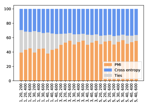
Figure 2: The average win rates of our PMI score and the test score benchmark. The orange bars represent the win rates or our PMI score, the blue bars represent the win rates of the benchmark (selection based on test score), and the gray bars represent the rates of ties. The label under the bar indicates $K,N_{T},M$.

Table 3: The generalization errors of the classifiers generated by our PMI score and the test score benchmark. The first column presents the outcomes when using our PMI score, the second column presents the results when using the benchmark, and the third column displays their differences.

$K,N_{T},M$	PMI score	Cross entropy	Difference
$1,20,200$	0.7699	0.7677	0.0022
$1,20,400$	0.7696	0.7670	0.0026
$1,20,600$	0.7677	0.7647	0.0030
$1,30,200$	0.7757	0.7738	0.0019
$1,30,400$	0.7761	0.7743	0.0018
$1,30,600$	0.7737	0.7713	0.0024
$1,40,200$	0.7784	0.7773	0.0011
$1,40,400$	0.7753	0.7740	0.0014
$1,40,600$	0.7773	0.7758	0.0015
$3,20,200$	0.7735	0.7712	0.0022
$3,20,400$	0.7747	0.7714	0.0033
$3,20,600$	0.7719	0.7682	0.0038
$3,30,200$	0.7781	0.7761	0.0020
$3,30,400$	0.7791	0.7763	0.0028
$3,30,600$	0.7758	0.7727	0.0032
$3,40,200$	0.7793	0.7774	0.0018
$3,40,400$	0.7794	0.7771	0.0023
$3,40,600$	0.7790	0.7762	0.0028
$5,20,200$	0.7749	0.7733	0.0016
$5,20,400$	0.7750	0.7724	0.0027
$5,20,600$	0.7721	0.7690	0.0031
$5,30,200$	0.7764	0.7745	0.0019
$5,30,400$	0.7782	0.7756	0.0026
$5,30,600$	0.7786	0.7755	0.0031
$5,40,200$	0.7804	0.7785	0.0018
$5,40,400$	0.7826	0.7804	0.0022
$5,40,600$	0.7782	0.7752	0.0030

Dataset selection with small test sets.

We assess the effectiveness of our PMI score in identifying high-quality datasets. We simulate a scenario where a data buyer seeks to evaluate data purchasing options from multiple providers using a small test set. We select the top $K$ datasets based on our PMI score and compare it against the benchmark method using test score. The two methods are compared by training a model on the selected datasets and evaluating its generalization error on a large test set. Our PMI dataset score consistently outperforms the benchmark across various settings by achieving lower average generalization error (Table 3) and a win rate of around $60\%$ (Figure 2).

In addition, the observed disparity between the two methods suggests that the PMI dataset score might be more robust to overfitting, meaning that the PMI dataset score is less likely to select datasets biased towards the small test set and result in higher generalization error of trained models. Specifically, in Table 3, the gap between the two methods widens as the number of candidate datasets $M$ increases; similarly in Figure 2, the win rate of our PMI score increases as $M$ increases. This could be due to the higher risk of overfitting to the small test set when we have a larger pool of candidate datasets, thus accentuating the advantages of the PMI score. Moreover, the gap decreases as we have a larger test set, i.e., when $N_{T}$ increases. This is likely because having more testing data helps mitigate overfitting to the small test set.

7 Discussion

As data markets become more prevalent, how to disincentivize data manipulation is a critical open challenge. Here we propose a new dataset scoring mechanism that is provably truthful. The focus of this work is to lay the theoretical and conceptual foundations of truthful dataset scoring; empirical applications and validations of this approach is an interesting direction of future work. It is also interesting to consider which of our modeling assumptions can potentially be broadened. Preliminarily, the impossibility theorems we provide in Appendix B.2 suggests that it could be challenging to have a meaningful and truthful dataset measure when there the data providers knows more about the setting than the data collector.

Appendix A Motivation for truthfulness

The example is inspired by Chaudhuri et al. [2023] and we mostly adopt their setup. Consider binary classification of examples $(x,y)$, where instances $x\in\mathbb{R}$ and $y\in\{+1,-1\}$. Assume that instances with label $+1$ are drawn independently from the Gaussian distribution $\mathcal{N}(1,1)$ and the instances with label $-1$ are drawn independently from $\mathcal{N}(-1,1)$. Suppose we have a test dataset that can be used for data evaluation and the test dataset consists of $50\%$ positive instances (with label $+1$) and $50\%$ negative instances (with label $-1$), and this percentage is publicly known. Consider a data provider who observes $90\%$ positive instances and $10\%$ negative instances.

Suppose we evaluate a dataset by training a classifier on the dataset and evaluating its test error. We consider classifiers $h_{b}(\cdot)$ that can be represented by a number $b$ and classifies $x\geq b$ as positive instances and $x\leq b$ as negative instances, i.e., $h_{b}(x)=+1$ if $x\geq b$ and $h_{b}(x)=-1$ otherwise. And we consider loss function $l(h_{b}(x),y)=-h_{b}(x)\cdot y$. Then the expected loss of a classifier on the test dataset is equal to

$$L(h_{b})=\frac{1}{2}\Pr(x_{+1}\leq b)+\frac{1}{2}\Pr(x_{-1}\geq b)=\Phi(b-1)+(1-\Phi(b+1)),$$

where $\Phi(\cdot)$ is the CDF of the standard normal distribution. Then we have the following fact.

Fact 1.

The expected loss on the test distribution is minimized by $h_{0}$, and $L(h_{b})$ is an increasing function of $|b|$ when $b<0$.

Following Chaudhuri et al. [2023], we assume that the classifier trained on a dataset $\{(x_{i},y_{i})\}_{i=1}^{n}$ is the maximum-margin classifier, which in this example is $h_{b^{*}}$ with $b^{*}=\frac{1}{2}(\max_{i:y_{i}=-1}x_{i}+\min_{i:y_{i}=+1}x_{i})$ equal to the mean of the maximum training point with a negative label and the minimum training point with a positive label. Then we only need to prove that with high probability, the maximum-margin classifier trained on a dataset with $90\%$ positive instances and $10\%$ negative instances will have $b^{*}<0$, so that the data provider can remove the minimum positive point to increase $b^{*}$ and thus reduces $L(h_{b^{*}})$. To prove that $b^{*}<0$ with high probability, we use the following result from Chaudhuri et al. [2023].

Lemma A.1.

Suppose $x_{1},\dots,x_{n}$ are scalar drawn i.i.d. from the standard normal distribution. Then for all $n>n_{0}$, for every $\delta\in(0,1)$, with probability $1-\delta$,

$$\max x_{i}\in\left[X_{\max}(n,\delta)-c(n,\delta),X_{\max}(n,\delta)+C(n,\delta)\right],$$

where $X_{\max}(n,\delta)=\sqrt{2\log n}-\frac{\log\log n+\log(4\pi)}{\sqrt{2\log n}}$, $c(n,\delta)=\frac{\log\log(6/\delta)}{\sqrt{2\log n}}$, and $C(n,\delta)=\frac{\log(6/\delta)}{\sqrt{2\log n}}$.

When a dataset contains $p$ positive instances and $m$ negative instances with $p\gg m$, then with high probability, we will have the maximum negative point very close to $\sqrt{2\log m}$ and the minimum positive point very close to $-\sqrt{2\log p}$, and we have their sum smaller than $0$ when $p\gg m$, which completes our proof.

Appendix B Impossibility results

B.1 Ex-post truthfulness

In our truthfulness definition (Definition 2.3), we assume that the data provider is uncertain about the underlying true ${\bm{\theta}}$ and the expected score is computed based on the data provider’s posterior belief $p({\bm{\theta}}|D=d)$. One may wonder whether truthfulness can be achieved if the data provider knows the true underlying ${\bm{\theta}}$, which we term ex-post truthfulness.

Definition B.1 (Ex-post truthfulness).

A data valuation metric $U(\cdot)$ is ex-post truthful if it is truthful conditional on ${\bm{\theta}}$, i.e., for any $d^{\prime},d\in\mathcal{D},\gamma\in\Theta$,

$$\mathbb{E}_{T}[U(d^{\prime},T)|D=d,{\bm{\theta}}=\gamma]\leq\mathbb{E}_{T}[U(d,T)|D=d,{\bm{\theta}}=\gamma].$$ (2)

Ex-post truthfulness can be interpreted as honest reporting in hindsight: the data provider will not regret truthful reporting after seeing the training results.

However, this stronger definition of truthfulness cannot be achieved in a non-trivial way. We show that the only ex-post truthful metric is a simplistic function that yields a constant expected score irrespective of the reported dataset. Evidently, this metric is not desirable as it fails to distinguish between authentic and fabricated datasets.

Proposition B.2.

Assuming that the evaluated dataset $D$ and the test dataset $T$ are independent conditioning on $\theta$, if a data valuation metric $U(\cdot)$ is ex-post truthful, then it must have for any possible $d,d^{\prime}\in\mathcal{D},\gamma\in\Theta$,

$$\mathbb{E}_{T}[U(d^{\prime},T)|D=d,{\bm{\theta}}=\gamma]=\mathbb{E}_{T}[U(d,T)|D=d,{\bm{\theta}}=\gamma].$$

Proof.

The key observation is that the conditional distribution of the test dataset $T$ given ${\bm{\theta}}=\gamma$ is the same no matter what dataset $D$ is observed by the data provider, i.e.,

$$p(T|D=d,{\bm{\theta}}=\gamma)=p(T|{\bm{\theta}}=\gamma).$$

Therefore, the condition of ex-post truthful (2) is equivalent to

$$\mathbb{E}_{T}[U(d^{\prime},T)|{\bm{\theta}}=\gamma]\leq\mathbb{E}_{T}[U(d,T)|{\bm{\theta}}=\gamma],\text{ for any }d^{\prime},d\in\mathcal{D},\gamma\in\Theta,$$

which implies

$$\mathbb{E}_{T}[U(d^{\prime},T)|{\bm{\theta}}=\gamma]=\mathbb{E}_{T}[U(d,T)|{\bm{\theta}}=\gamma],\text{ for any }d^{\prime},d\in\mathcal{D},\gamma\in\Theta,$$

and this is equivalent to

$$\mathbb{E}_{T}[U(d^{\prime},T)|D=d,{\bm{\theta}}=\gamma]=\mathbb{E}_{T}[U(d,T)|D=d,{\bm{\theta}}=\gamma],\text{ for any possible }d,d^{\prime}\in\mathcal{D},\gamma\in\Theta.$$

∎

B.2 Unknown provider observations

We assume that all of the data provider’s observations about ${\bm{\theta}}$ are included in the dataset $D$. If the data provider observes other information about ${\bm{\theta}}$ that is not reported to the data collector, then in general, it is impossible to design meaningful truthful data valuation functions.

We demonstrate the impossibility using the example in Section 4.1. Suppose in the univariate Gaussian example, the provider is able to observe the shift $\Delta$ but the collector cannot, and the provider does not include the value of $\Delta$ in the dataset, then we can prove that in this case, the only valuation function that guarantees truthful reporting are the functions that ignore the mean $\overline{x}_{D}$ and only depend on $N_{D}$ and $T$.

Proposition B.3.

Suppose in the univariate Gaussian example in Section 4.1, the data provider observed the shift $\Delta$ while the data collector does not, and the data provider only reports $D$, then the only valuation functions that guarantee truthful reporting are the valuation functions that ignore $\overline{x}_{D}$ and assign an expected score based on $N_{D}$. More specifically, let $\overline{U}(d,w_{t})$ be the expected score when the provider reports $d$ and the true mean $w_{T}=w_{t}$, then we must have

$$\overline{U}(d,w_{t})=\overline{U}(d^{\prime},w_{t}),\quad\text{for all }w_{t},\text{ and }d,d^{\prime}\text{ with the same size.}$$

Proof.

Suppose the provider observes $d$ with size $N_{d}$. Suppose the true underlying bias is $\delta$, which is observed by the provider but not the collector. Then the provider’s posterior about $w_{D}$ is $p(w_{D}|d)=\mathcal{N}(\mu_{d},\sigma_{d}^{2})$ with $\mu_{d}=\frac{N_{d}\cdot\overline{x}_{d}/\sigma^{2}}{N_{d}/\sigma^{2}+1/\sigma_{0}^{2}}$, $\sigma_{d}^{2}=\frac{1}{N_{d}/\sigma^{2}+1/\sigma_{0}^{2}}$ and $\overline{x}_{d}=\sum_{i}x_{d}^{(i)}/N_{d}$. Then the provider’s posterior about ${\bm{\theta}}$ is $p({\bm{\theta}}|d)=\mathcal{N}(\mu_{d}+\delta,\sigma_{d}^{2})$.

Consider another scenario where the provider observes $d^{\prime}$ with the same size $N_{d}$ with the true underlying bias $\delta^{\prime}$ satisfying

$$\frac{N_{d}\cdot\overline{x}_{d}/\sigma^{2}}{N_{d}/\sigma^{2}+1/\sigma_{0}^{2}}+\delta=\frac{N_{d}\cdot\overline{x}_{d^{\prime}}/\sigma^{2}}{N_{d}/\sigma^{2}+1/\sigma_{0}^{2}}+\delta^{\prime}.$$ (3)

Then in this scenario, the provider’s posterior belief about ${\bm{\theta}}$ will be equal to $\mathcal{N}(\mu_{d}+\delta,\sigma_{d}^{2})$ as well.

But the data collector cannot distinguish the two scenario because she cannot observe $\delta$. As a result, the provider’s expected score will be the same in the two scenarios for any report $d^{\prime\prime}$. But the truthful reports in the two scenarios are different. Let $\overline{U}(d,w_{t})$ be the expected score when the provider reports $d$ and $T$’s true mean $w_{T}=w_{t}$. Then we should have

$$\int\overline{U}(d,w_{t})\cdot\mathcal{N}(w_{t}|\mu_{d}+\delta,\sigma_{d}^{2})\,dw_{t}\geq\int\overline{U}(d^{\prime},w_{t})\cdot\mathcal{N}(w_{t}|\mu_{d}+\delta,\sigma_{d}^{2})\,dw_{t}$$

due to the truthfulness requirement in the first scenario, and

$$\int\overline{U}(d,w_{t})\cdot\mathcal{N}(w_{t}|\mu_{d}+\delta,\sigma_{d}^{2})\,dw_{t}\leq\int\overline{U}(d^{\prime},w_{t})\cdot\mathcal{N}(w_{t}|\mu_{d}+\delta,\sigma_{d}^{2})\,dw_{t}$$

due to the truthfulness requirement in the second scenario, which gives

$$\int\overline{U}(d,w_{t})\cdot\mathcal{N}(w_{t}|\mu_{d}+\delta,\sigma_{d}^{2})\,dw_{t}=\int\overline{U}(d^{\prime},w_{t})\cdot\mathcal{N}(w_{t}|\mu_{d}+\delta,\sigma_{d}^{2})\,dw_{t}.$$

And this should hold for any $\delta\in\mathbb{R}$. Therefore we should have $\overline{U}(d,w_{t})\equiv\overline{U}(d^{\prime},w_{t})$. And this should hold for any $d,d^{\prime}$ with the same size, which completes our proof. ∎

Appendix C Missing proofs in Section 3

C.1 Proof of Theorem 2.10

For completeness, we provide a stand-alone proof for Theorem 2.10.

Theorem C.1 (Kong and Schoenebeck [2018b], Chen et al. [2020]).

Let $D$ and $T$ be two datasets that are independent conditional on ${\bm{\theta}}$, i.e.,

$$p(D,T|{\bm{\theta}})=p(D|{\bm{\theta}})p(T|{\bm{\theta}}),$$

then the valuation function

$$U(d,t)=\log\int_{\bm{\theta}}p({\bm{\theta}}|D=d)p({\bm{\theta}}|T=t)/p({\bm{\theta}})\,d{\bm{\theta}}.$$

is truthful.

Proof.

This is basically because when $D$ and $T$ are conditionally independent, we have

$$U(d^{\prime},t) =\log\int_{\bm{\theta}}\frac{p({\bm{\theta}}|D=d^{\prime})p({\bm{\theta}}|T=t)}{p({\bm{\theta}})}\,d{\bm{\theta}}$$

$$=\log\int_{\bm{\theta}}\frac{p(d^{\prime}|{\bm{\theta}})p(t|{\bm{\theta}})p({\bm{\theta}})}{p(d^{\prime})p(t)}\,d{\bm{\theta}}$$

$$=\log\frac{\int_{\bm{\theta}}p(d^{\prime},t,{\bm{\theta}})\,d{\bm{\theta}}}{p(d^{\prime})p(t)}$$

$$=\log\frac{p(d^{\prime},t)}{p(d^{\prime})p(t)}$$

$$=\log\frac{p(t|D=d^{\prime})}{p(t)}$$

$$=\log p(t|D=d^{\prime})-\log p(t),$$

which is just the log scoring rule. If the data provider manipulates the dataset and report $f(d)=d^{\prime}\neq d$, then we have

$$\mathbb{E}_{T}[U(d,T)|D=d]-\mathbb{E}_{T}[U(d^{\prime},T)|D=d]$$

$$= \sum_{t\in\mathcal{T}}p(t|D=d)\log p(t|D=d)-\sum_{t\in\mathcal{T}}p(t|D=d)\log p(t|D=d^{\prime})$$

$$= \sum_{t\in\mathcal{T}}p(t|D=d)\log\frac{p(t|D=d)}{p(t|D=d^{\prime})}$$

$$= \ D_{KL}\big{(}p(t|D=d),p(t|D=d^{\prime})\big{)}$$

$$\geq \ 0.$$

∎

This also proves Proposition 2.8.

Chen et al. [2020] proposed a theoretical framework for computing this integral score for exponential family distributions.

Definition C.2 (Exponential family Murphy [2012]).

A likehihood function $p({\mathbf{x}}|{\bm{\theta}})$, for ${\mathbf{x}}=(x_{1},\dots,x_{n})\in\mathcal{X}^{n}$ and ${\bm{\theta}}\in\Theta\subseteq\mathbb{R}^{m}$ is said to be in the exponential family in canonical form if it is of the form

$$p({\mathbf{x}}|{\bm{\theta}})=\frac{1}{Z({\bm{\theta}})}h({\mathbf{x}})\exp\left[{\bm{\theta}}^{T}{\bm{\phi}}({\mathbf{x}})\right]\quad\text{ or }\quad p({\mathbf{x}}|{\bm{\theta}})=h({\mathbf{x}})\exp\left[{\bm{\theta}}^{T}{\bm{\phi}}({\mathbf{x}})-A({\bm{\theta}})\right]$$ (4)

Here $\bm{\phi}(x)\in\mathbb{R}^{m}$ is called a vector of sufficient statistics, $Z({\bm{\theta}})=\int_{\mathcal{X}^{n}}h({\mathbf{x}})\exp\left[{\bm{\theta}}^{T}{\bm{\phi}}({\mathbf{x}})\right]$ is called the partition function, $A({\bm{\theta}})=\ln Z({\bm{\theta}})$ is called the log partition function.

If the posterior distributions $p({\bm{\theta}}|{\mathbf{x}})$ are in the same probability distribution family as the prior probability distribution $p({\bm{\theta}})$, the prior and posterior are then called conjugate distributions, and the prior is called a conjugate prior.

Definition C.3 (Conjugate prior for the exponential family Murphy [2012]).

For a likelihood function in the exponential family $p({\mathbf{x}}|{\bm{\theta}})=h({\mathbf{x}})\exp\left[{\bm{\theta}}^{T}{\bm{\phi}}({\mathbf{x}})-A({\bm{\theta}})\right]$. The conjugate prior for ${\bm{\theta}}$ with parameters $\nu_{0},\overline{\bm{\tau}}_{0}$ is of the form

$$p({\bm{\theta}})=\mathcal{P}({\bm{\theta}}|\nu_{0},\overline{\bm{\tau}}_{0})=g(\nu_{0},\overline{\bm{\tau}}_{0})\exp\left[\nu_{0}{\bm{\theta}}^{T}\overline{\bm{\tau}}_{0}-\nu_{0}A({\bm{\theta}})\right].$$ (5)

Let $\overline{\bm{s}}=\frac{1}{n}\sum_{i=1}^{n}\bm{\phi}(x_{i})$. Then the posterior of ${\bm{\theta}}$ can be represented in the same form as the prior

$$p({\bm{\theta}}|{\mathbf{x}})\propto\exp\left[{\bm{\theta}}^{T}(\nu_{0}\overline{\bm{\tau}}_{0}+n\overline{\bm{s}})-(\nu_{0}+n)A({\bm{\theta}})\right]=\mathcal{P}\big{(}{\bm{\theta}}|\nu_{0}+n,\frac{\nu_{0}\overline{\bm{\tau}}_{0}+n\overline{\bm{s}}}{\nu_{0}+n}\big{)},$$

where $\mathcal{P}\big{(}{\bm{\theta}}|\nu_{0}+n,\frac{\nu_{0}\overline{\bm{\tau}}_{0}+n\overline{\bm{s}}}{\nu_{0}+n}\big{)}$ is the conjugate prior with parameters $\nu_{0}+n$ and $\frac{\nu_{0}\overline{\bm{\tau}}_{0}+n\overline{\bm{s}}}{\nu_{0}+n}$.

Then if the prior and the posteriors are in an exponential family, the integral PMI score can be expressed as follows using the normalization function $g(\cdot)$.

Lemma C.4.

If the model distributions are in an exponential family, so that the prior and all the posterior of ${\bm{\theta}}$ can be written in the form

$$p({\bm{\theta}})=\mathcal{P}({\bm{\theta}}|\nu_{0},\overline{\bm{\tau}}_{0})=g(\nu_{0},\overline{\bm{\tau}}_{0})\exp\left[\nu_{0}{\bm{\theta}}^{T}\overline{\bm{\tau}}_{0}-\nu_{0}A({\bm{\theta}})\right],$$

$p({\bm{\theta}}|D)=\mathcal{P}({\bm{\theta}}|\nu_{D},\overline{\bm{\tau}}_{D})$ and $p({\bm{\theta}}|T)=\mathcal{P}({\bm{\theta}}|\nu_{T},\overline{\bm{\tau}}_{T})$, then the pointwise mutual information can be expressed as

$$PMI(D,T)=\frac{g(\nu_{D},\overline{\bm{\tau}}_{D})g(\nu_{T},\overline{\bm{\tau}}_{T})}{g(\nu_{0},\overline{\bm{\tau}}_{0})g(\nu_{D}+\nu_{T}-\nu_{0},\frac{\nu_{D}\overline{\bm{\tau}}_{D}+\nu_{T}\overline{\bm{\tau}}_{T}-\nu_{0}\overline{\bm{\tau}}_{0}}{\nu_{D}+\nu_{T}-\nu_{0}})}.$$

However, finding the function $g(\cdot)$ is not straightforward and may involve solving a complex integral. Chen et al. [2020] did not provide a practical method to find the $g(\cdot)$ function. In particular, it is not clear how to use their framework for Gaussian models, and their analysis for the simple univariate Gaussian case ([Chen et al., 2020] Appendix C.4) is not correct. For Gaussian models, the normalization function $g(\cdot)$ should depend on the mean $\mu$ as well (as shown in our Proposition 4.1), but their solution only depends on the variance. As a result, their conclusion that the PMI score is not sensitive to mean shift is wrong. (See our Section 4.1 and Figure 1 for the correct solution).

C.2 Proof of Theorem 3.1

To prove the theorem, we first prove the following lemma.

Lemma C.5.

Let $D$ and $T$ be two random variables that are independent conditional on random variable ${\bm{\theta}}$, that is, $p(D,T|{\bm{\theta}})=p(D|{\bm{\theta}})p(T|{\bm{\theta}})$. Then we have for any $\eta\in\Theta$, $d\in\mathcal{D}$, and $t\in\mathcal{T}$,

$$\frac{p(T=t|D=d)}{p(T=t)}=\frac{p({\bm{\theta}}=\eta|D=d)\cdot p({\bm{\theta}}=\eta|T=t)}{p({\bm{\theta}}=\eta)\cdot p({\bm{\theta}}=\eta|D=d,T=t)}.$$

The proof of Lemma C.5 mainly relies on Bayes’ rule and the conditional independence condition.

Proof.

Since $D,T$ are independent conditional on ${\bm{\theta}}$, for any $\eta\in\Theta$ we have

$$p({\bm{\theta}}=\eta|D=d,T=t)$$

$$=\frac{p(D=d,T=t|{\bm{\theta}}=\eta)\cdot p({\bm{\theta}}=\eta)}{p(D=d,T=t)}$$

$$=\frac{p(D=d|{\bm{\theta}}=\eta)\cdot p(T=t|{\bm{\theta}}=\eta)\cdot p({\bm{\theta}}=\eta)}{p(D=d,T=t)}$$

$$=\frac{p({\bm{\theta}}=\eta|D=d)\cdot p({\bm{\theta}}=\eta|T=t)\cdot p(D=d)\cdot p(T=t)}{p({\bm{\theta}}=\eta)\cdot p(D=d,T=t)}.$$

Then we have

$$\frac{p({\bm{\theta}}=\eta|D=d)\cdot p({\bm{\theta}}=\eta|T=t)}{p({\bm{\theta}}=\eta)\cdot p({\bm{\theta}}=\eta|D=d,T=t)} =\frac{p(D=d,T=t)}{p(D=d)\cdot p(T=t)}$$

$$=\frac{p(T=t|D=d)}{p(T=t)}.$$

∎

With this equation, we can apply the logarithmic scoring rule to get a truthful valuation function, which gives the valuation function in Theorem 3.1. The proof is as follows.

Proof.

According to Lemma C.5, $U(d,t)=\log p(T=t|D=d)/P(T=t)$. Then the expected score is maximized by reporting $d$ because

$$\mathbb{E}_{T}[U_{\eta}(d,T)|D=d]-\mathbb{E}_{T}[U_{\eta}(d^{\prime},T)|D=d]$$

$$= \int_{t}p(t|D=d)\log p(t|D=d)\,dt-\int_{t}p(t|D=d)\log p(t|D=d^{\prime})\,dt$$

$$= \int_{t}p(t|D=d)\log\frac{p(t|D=d)}{p(t|D=d^{\prime})}\,dt$$

$$= \ D_{KL}\big{(}p(t|D=d),p(t|D=d^{\prime})\big{)}$$

$$\geq \ 0.$$

And when truthful reporting, the expected score $\mathbb{E}[U_{\eta}(D,T)]$ is just the Shannon mutual information $I(D,T)=\mathbb{E}_{D,T}\left[\log\frac{p(D,T)}{p(D)p(T)}\right]$. ∎

C.3 Extension: release sample data

In this section, we adapt our data valuation method to support test data preview: the data collector releases a random sample from the test dataset so that the data provider can conduct an initial evaluation of their own data. We consider the following timeline.

1. The data collector posts a data valuation metric $U(d,t)$ for $d\in\mathcal{D},t\in\mathcal{T}$.

2. Nature draws ${\bm{\theta}}\sim p({\bm{\theta}})$ and the data collector draws a test dataset $T\sim p(T|{\bm{\theta}})$ and the data provider observes a dataset $D\sim p(D|{\bm{\theta}})$.

3. The data collector releases a random sample $S\subseteq T$.

4. After seeing the metric $U(\cdot)$, the dataset $D$, and the released sample $S$, the data provider chooses a dataset $D^{\prime}$ and submits it to the data collector.

5. The data collector uses the posted metric to evaluate the submitted dataset, so the data provider receives a score of $U(D^{\prime},T)$.

Theorem C.6.

Suppose $D$, $S$, and $T\setminus S$ are independent conditional on ${\bm{\theta}}$ and the data collector is able to compute the posterior of ${\bm{\theta}}$ given any dataset (including the union of test data and evaluated data). Then when we use the valuation function

$$U_{\eta}(d,t)=\log\frac{p({\bm{\theta}}=\eta|S,D=d)\cdot p({\bm{\theta}}=\eta|T=t)}{p({\bm{\theta}}=\eta|S)\cdot p({\bm{\theta}}=\eta|D=d,T=t)},$$

the data provider’s expected score is always maximized by truthful reporting, after seeing the sample test data $S$. Furthermore, the expectation of $U_{\eta}(\cdot)$ is equal to the conditional mutual information of $D$ and $R$ given $S$ when the data provider reports truthfully, that is, $\mathbb{E}[U_{\eta}(D,T)|S]=I(D,T|S)$.

To prove the theorem, we first prove two lemmas.

Lemma C.7.

Let $D$, $S$, and $R$ be random variables that are independent conditional on random variable ${\bm{\theta}}$, that is, $p(D,S,R|{\bm{\theta}})=p(D|{\bm{\theta}})p(S|{\bm{\theta}})p(R|{\bm{\theta}})$. Then we have

$$p(D,R|S,{\bm{\theta}})=p(D|S,{\bm{\theta}})p(R|S,{\bm{\theta}}).$$ (6)

Proof.

It suffices to prove that $p(D,R|S,{\bm{\theta}})=p(D,R|{\bm{\theta}})$, $p(D|S,{\bm{\theta}})=p(D|{\bm{\theta}})$, and $p(R|S,{\bm{\theta}})=p(R|{\bm{\theta}})$, because then Equation (6) will be equivalent to the conditional independence condition. We prove $p(D|S,{\bm{\theta}})=p(D|{\bm{\theta}})$ and the other two equations are similar. Due to conditional independence, we have

$$p(D,S|{\bm{\theta}})=p(S|{\bm{\theta}})\cdot p(D|{\bm{\theta}}).$$

Divide both side by $p(S|{\bm{\theta}})$ we get $p(D|S,{\bm{\theta}})=p(D|{\bm{\theta}})$, which completes our proof. ∎

Lemma C.8.

Let $D$, $S$, and $R$ be random variables that are independent conditional on random variable ${\bm{\theta}}$, that is, $p(D,S,R|{\bm{\theta}})=p(D|{\bm{\theta}})p(S|{\bm{\theta}})p(R|{\bm{\theta}})$. Then we have for any $\eta\in\Theta$,

$$\frac{p(R|D,S)}{p(R|S)}=\frac{p({\bm{\theta}}=\eta|S,D)\cdot p({\bm{\theta}}=\eta|S,R)}{p({\bm{\theta}}=\eta|S)\cdot p({\bm{\theta}}=\eta|S,D,R)}.$$

Proof.

Since $D,S,R$ are independent conditional on ${\bm{\theta}}$, for any $\eta\in\Theta$ we have

$$p({\bm{\theta}}=\eta|S,D,R)$$

$$=\frac{p(D,R|S,{\bm{\theta}}=\eta)\cdot p({\bm{\theta}}=\eta|S)}{p(D,R|S)}$$

$$=\frac{p(D|S,{\bm{\theta}}=\eta)\cdot p(R|S,{\bm{\theta}}=\eta)\cdot p({\bm{\theta}}=\eta|S)}{p(D,R|S)}$$

$$=\frac{p({\bm{\theta}}=\eta|S,D)\cdot p(D|S)\cdot p({\bm{\theta}}=\eta|S,R)\cdot p(R|S)}{p({\bm{\theta}}=\eta|S)\cdot p(D,R|S)}$$

Then we have

$$\frac{p({\bm{\theta}}=\eta|S,D)\cdot p({\bm{\theta}}=\eta|S,R)}{p({\bm{\theta}}=\eta|S)\cdot p({\bm{\theta}}=\eta|S,D,R)} =\frac{p(D,R|S)}{p(D|S)\cdot p(R|S)}$$

$$=\frac{p(R|D,S)}{p(R|S)}.$$

∎

Then we are ready to prove the theorem.

Proof.

The expected score is maximized by reporting $d$ because

$$\mathbb{E}_{T}[U_{\eta}(d,T)|D=d,S=s]-\mathbb{E}_{T}[U_{\eta}(d^{\prime},T)|D=d,S=s]$$

$$= \int_{t}p(t|d,s)\log p(t|d,s)\,dt-\int_{t}p(t|d,s)\log p(t|d^{\prime},s)\,dt$$

$$= \int_{t}p(t|d,s)\log\frac{p(t|d,s)}{p(t|d^{\prime},s)}\,dt$$

$$= \ D_{KL}\big{(}p(t|d,s),p(t|d^{\prime},s)\big{)}$$

$$\geq \ 0.$$

And when truthful reporting, the expected score $\mathbb{E}[U_{\eta}(D,T)|S]$ is just the Shannon mutual information $I(D,T|S)$. ∎

Appendix D Missing proofs in Section 4

D.1 Proof of  Proposition 4.1

We consider Gaussian models with posteriors $p({\bm{\theta}}|D=d)=\mathcal{N}(\mu_{a},\Sigma_{a})$, $p({\bm{\theta}}|T=t)=\mathcal{N}(\mu_{b},\Sigma_{b})$, $p({\bm{\theta}}|D=d,T=t)=\mathcal{N}(\mu_{ab},\Sigma_{ab})$, and the prior $p({\bm{\theta}})=\mathcal{N}(\mu_{0},\Sigma_{0})$. Then the PMI score with $\eta=0$ is equal to

$$U_{0}(d,t)= \frac{1}{2}\left(\log\frac{\det(\Sigma_{0})\det(\Sigma_{ab})}{\det(\Sigma_{a})\det(\Sigma_{b})}+\mu_{0}^{T}\Sigma_{0}^{-1}\mu_{0}+\mu_{ab}^{T}\Sigma_{ab}^{-1}\mu_{ab}-\mu_{a}^{T}\Sigma_{a}^{-1}\mu_{a}-\mu_{b}^{T}\Sigma_{b}^{-1}\mu_{b}\right).$$ (7)

Then it suffices to prove that $\Sigma_{ab}=(\Sigma_{a}^{-1}+\Sigma_{b}^{-1}-\Sigma_{0}^{-1})^{-1}$ and $\mu_{ab}=\Sigma_{ab}\left(\Sigma_{a}^{-1}\mu_{a}+\Sigma_{b}^{-1}\mu_{b}-\Sigma_{0}^{-1}\mu_{0}\right)$. Due to conditional independence and according to the proof of Lemma C.5, we have

$$p({\bm{\theta}}|d,t) \propto\frac{p({\bm{\theta}}|d)p({\bm{\theta}}|t)}{p({\bm{\theta}})}$$

$$=\frac{\mathcal{N}({\bm{\theta}};\mu_{a},\Sigma_{a})\mathcal{N}({\bm{\theta}};\mu_{b},\Sigma_{b})}{\mathcal{N}({\bm{\theta}};\mu_{0},\Sigma_{0})}$$

$$\propto\exp\Big{(}-\frac{1}{2}g({\bm{\theta}})\Big{)}$$

where

$$g({\bm{\theta}}) :=({\bm{\theta}}-\mu_{a})^{T}\Sigma_{a}^{-1}({\bm{\theta}}-\mu_{a})+({\bm{\theta}}-\mu_{b})^{T}\Sigma_{b}^{-1}({\bm{\theta}}-\mu_{b})-({\bm{\theta}}-\mu_{0})^{T}\Sigma_{0}^{-1}({\bm{\theta}}-\mu_{0})$$

Here, $g({\bm{\theta}})$ can be further simplified as $g({\bm{\theta}})=({\bm{\theta}}-\widetilde{\mu})^{T}\widetilde{\Sigma}^{-1}({\bm{\theta}}-\widetilde{\mu})+Z_{2}$ where

$$\widetilde{\Sigma} =(\Sigma_{a}^{-1}+\Sigma_{b}^{-1}-\Sigma_{0}^{-1})^{-1}$$

$$\widetilde{\mu} =\widetilde{\Sigma}\left(\Sigma_{a}^{-1}\mu_{a}+\Sigma_{b}^{-1}\mu_{b}-\Sigma_{0}^{-1}\mu_{0}\right)$$

$$Z_{2} =\mu_{a}^{T}\Sigma_{a}^{-1}\mu_{a}+\mu_{b}^{T}\Sigma_{b}^{-1}\mu_{b}-\mu_{0}^{T}\Sigma_{0}^{-1}\mu_{0}-\widetilde{\mu}^{T}\widetilde{\Sigma}^{-1}\widetilde{\mu}.$$

Then $p({\bm{\theta}}|d,t)$ must be the Gaussian distribution with mean $\widetilde{\mu}$ and covariance matrix $\widetilde{\Sigma}$.

D.2 Examples in Section 4.1

Normally-distributed data with mean shifts.

We first show how to evaluate normally distributed data $D$ with a test dataset $T$ that has an unknown distributional shift. For simplicity, we illustrate the simple case where the two datasets consist of numbers drawn from two univariate Gaussians with a shift in the mean, and the multivariate case is entirely similar.

Suppose the data provider observes a dataset $D$ that contains $N_{D}$ i.i.d. data points $x_{D}^{(1)},\dots,x_{D}^{(N_{D})}$ drawn from $\mathcal{N}(w_{D},\sigma^{2})$ with unknown $w_{D}$, and the data collector observes a test dataset $T$ that contains $N_{T}$ i.i.d. data points $x_{T}^{(1)},\dots,x_{T}^{(N_{T})}$ drawn from a correlated distribution $\mathcal{N}(w_{T},\sigma^{2})$ with an unknown shift in the mean $w_{T}=w_{D}+\Delta$. We assume that the following information is publicly known: the prior distribution of the shift $\Delta\sim\mathcal{N}(\mu_{\Delta},\sigma_{\Delta}^{2})$, the prior of $w_{D}\sim\mathcal{N}(0,\sigma_{0}^{2})$, $w_{D}$ and $\Delta$ are independent, and thus we have the prior $w_{T}\sim\mathcal{N}(\mu_{\Delta},\sigma_{0}^{2}+\sigma_{\Delta}^{2})$.

To use our PMI score, we first need to pick the parameter $\theta$ to compute the posteriors. We can either pick $\theta=w_{D}$ or $\theta=w_{T}$ because $D$ and $T$ will be independent conditioning on any of them. WLOG and for simplicity, we choose $\theta=w_{T}$. Then by Proposition 4.1, to compute our score, we only need to find $p(\theta|D)$ and $p(\theta|T)$.

The posterior of $\theta$ given $T$ is easy to compute. The posterior of $\theta$ given $D$ is slightly more complicated. First of all, the posterior of $w_{D}$ given $D$ is easy to find, and let it be $p(w_{D}|D)=\mathcal{N}\left(\mu_{c},\,\sigma_{c}^{2}\right)$. Since $\Delta$ and $D$ are independent, we have $p(\Delta|D)=\mathcal{N}(\mu_{\Delta},\sigma_{\Delta}^{2})$. In addition, $\Delta$ and $w_{D}$ are independent conditioning on $D$. Therefore by the lemma of the sum of normally distributed random variables, we have $p(\theta|D)=p(w_{D}+\Delta|D)=\mathcal{N}(\mu_{c}+\mu_{\Delta},\sigma_{c}^{2}+\sigma_{\Delta}^{2})$. Then the PMI score can be computed using Proposition 4.1. In Figure 1, we plot the provider’s expected PMI score for different reports when $T$ contains one data point. See details in Appendix D.3.

Linear regression.

Consider Bayesian linear regression with likelihood function $p(y|{\mathbf{x}},{\bm{\theta}})=\mathcal{N}({\bm{\theta}}^{T}{\mathbf{x}},\sigma^{2})$ and prior $p({\bm{\theta}})=\mathcal{N}(\mu_{0},\Sigma_{0})$. Then according to Murphy [2012], given a dataset $(\mathbf{X},{\mathbf{y}})$, (where matrix $\mathbf{X}$ is the input data with each column being a data feature and vector ${\mathbf{y}}$ is the observed labels,) the posterior of ${\bm{\theta}}$ is a normal distribution $p({\bm{\theta}}|\mathbf{X},{\mathbf{y}})=\mathcal{N}(\mu,\,\Sigma)$ with $\Sigma^{-1}=\Sigma_{0}^{-1}+\frac{1}{\sigma^{2}}\mathbf{X}^{T}\mathbf{X}$ and $\mu=\Sigma\Sigma_{0}^{-1}\mu_{0}+\frac{1}{\sigma^{2}}\Sigma\mathbf{X}^{T}{\mathbf{y}}$. So as long as the data collector knows the prior distribution $\mathcal{N}(\mu_{0},\Sigma_{0})$ as well as the variance of the noise $\sigma^{2}$, the data collector can compute the posterior of ${\bm{\theta}}$ given any dataset, and our PMI score can be computed by Proposition 4.1. Note that we do not need to assume the distribution of the feature $p({\mathbf{x}}|{\bm{\theta}})$ and our PMI score can be used when the test data and the evaluated data have different feature distributions.

Logistic regression with Gaussian approximation.

Consider logistic regression with likelihood function $p(y|{\mathbf{x}},{\bm{\theta}})=\text{Ber}(y|\text{Sigm}({\bm{\theta}}^{T}{\mathbf{x}}))$, and consider Bayesian logistic regression with Gaussian approximation (see Murphy [2012] Chapter 8) where a Gaussian prior $p({\bm{\theta}})=\mathcal{N}(0,\Sigma_{0})$ is assumed. Then given a dataset $(\mathbf{X},{\mathbf{y}})$, (where matrix $\mathbf{X}$ is the input data with each column being a data feature and vector ${\mathbf{y}}$ is the observed labels,) the approximate posterior is given by $p({\bm{\theta}}|\mathbf{X},{\mathbf{y}})\approx\mathcal{N}(\mu,\Sigma)$ with

$$\mu=\arg\min_{\mathbf{w}}E({\mathbf{w}}),\quad\Sigma^{-1}=\nabla^{2}E({\mathbf{w}})|\mu,$$

where $E({\mathbf{w}})$ $=-(\log p({\mathbf{y}}|\mathbf{X},{\mathbf{w}})$ $+\log p({\mathbf{w}})).$ Then $\mu$ can be solved by gradient descent and the Hessian matrix $\Sigma^{-1}$ can be computed in closed form. In particular, if we pick $\Sigma_{0}=\mathbf{I}$, then we have $\Sigma^{-1}=\mathbf{X}^{T}\mathbf{S}\mathbf{X}+\mathbf{I}$, where $\mathbf{S}=\text{diag}\big{(}\text{Sigm}(\mu^{T}{\mathbf{x}}_{i})(1-\text{Sigm}(\mu^{T}{\mathbf{x}}_{i}))\big{)}$. Therefore as long as the data collector knows the prior $\mathcal{N}(0,\Sigma_{0})$, she will be able to compute the posterior given any dataset, and thus our PMI score can be computed by Proposition 4.1. Again, we do not need to assume the distribution of the feature $p({\mathbf{x}}|{\bm{\theta}})$ and our PMI score can be used when the test data and the evaluated data have different feature distributions.

D.3 Detailed calculation for Normally-distributed data with mean shifts

The posterior of $\theta$ given $T$ is easy to compute: we have $p(\theta|T)=p(w_{T}|T)=\mathcal{N}\left(\mu_{b},\,\sigma_{b}^{2}\right)$, with $\mu_{b}=\frac{N_{T}\cdot\overline{x}_{T}/\sigma^{2}+\mu_{\Delta}/(\sigma_{0}^{2}+\sigma_{\Delta}^{2})}{N_{T}/\sigma^{2}+1/(\sigma_{0}^{2}+\sigma_{\Delta}^{2})}$, $\sigma_{b}^{2}=\frac{1}{N_{T}/\sigma^{2}+1/(\sigma_{0}^{2}+\sigma_{\Delta}^{2})}$, and $\overline{x}_{T}=\sum_{i}x_{T}^{(i)}/N_{T}$. The posterior of $\theta$ given $D$ is slightly more complicated. First of all, the posterior of $w_{D}$ given $D$ is easy to find, $p(\theta-\Delta|D)=p(w_{D}|D)=\mathcal{N}\left(\mu_{c},\,\sigma_{c}^{2}\right)$ with $\mu_{c}=\frac{N_{D}\cdot\overline{x}_{D}/\sigma^{2}}{N_{D}/\sigma^{2}+1/\sigma_{0}^{2}}$, $\sigma_{c}^{2}=\frac{1}{N_{D}/\sigma^{2}+1/\sigma_{0}^{2}}$ and $\overline{x}_{D}=\sum_{i}x_{D}^{(i)}/N_{D}$. Since $\Delta$ and $D$ are independent, we have $p(\Delta|D)=\mathcal{N}(\mu_{\Delta},\sigma_{\Delta}^{2})$. In addition, $\Delta$ and $w_{D}$ are independent conditioning on $D$. Therefore by the lemma of the sum of normally distributed random variables, we have $p(\theta|D)=p(w_{D}+\Delta|D)=\mathcal{N}(\mu_{c}+\mu_{\Delta},\sigma_{c}^{2}+\sigma_{\Delta}^{2})$, which is equal to

$$p(\theta|D)=p(w_{D}+\Delta|D)=\mathcal{N}\left(\frac{N_{D}\cdot\overline{x}_{D}/\sigma^{2}}{N_{D}/\sigma^{2}+1/\sigma_{0}^{2}}+\mu_{\Delta},\,\frac{1}{N_{D}/\sigma^{2}+1/\sigma_{0}^{2}}+\sigma_{\Delta}^{2}\right).$$

For simplicity, we choose $\sigma^{2}=\sigma_{0}^{2}=\sigma_{\Delta}^{2}=1$. Then we have

$$p(\theta|T)=p(w_{T}|T)=\mathcal{N}\left(\frac{N_{T}\cdot\overline{x}_{T}+\mu_{\Delta}/2}{N_{T}+1/2},\,\frac{1}{N_{T}+1/2}\right),$$

and

$$p(\theta|D)=\mathcal{N}\left(\frac{N_{D}\cdot\overline{x}_{D}}{N_{D}+1}+\mu_{\Delta},\,\frac{1}{N_{D}+1}+1\right).$$

Then by Proposition 4.1, we have

$$U(D,T)=\frac{1}{2}\big{(}\log C(N_{D},N_{T})+V(\mu_{\Delta},N_{D},\overline{x}_{D},N_{T},\overline{x}_{T})\big{)},$$

with $C(N_{D},N_{T})=\frac{2(N_{D}+1)(N_{T}+1/2)/(N_{D}+2)}{(N_{D}+1)/(N_{D}+2)+N_{T}}$ and

$$V(\mu_{\Delta},N_{D},\overline{x}_{D},N_{T},\overline{x}_{T})= \mu_{\Delta}^{2}/2+\frac{\left(\frac{N_{D}\cdot\overline{x}_{D}}{N_{D}+2}+\frac{\mu_{\Delta}(N_{D}+1)}{N_{D}+2}+N_{T}\cdot\overline{x}_{T}\right)^{2}}{(N_{D}+1)/(N_{D}+2)+N_{T}}$$

$$-\left(\mu_{\Delta}+\frac{N_{D}\cdot\overline{x}_{D}}{N_{D}+1}\right)^{2}\cdot\frac{N_{D}+1}{N_{D}+2}-\frac{\left(N_{T}\cdot\overline{x}_{T}+\mu_{\Delta}/2\right)^{2}}{N_{T}+1/2}.$$

Appendix E Missing proofs in Section 5

E.1 Interpretation by pointwise mutual parameter information

Firstly, our score can be represented as $d$ and $t$’s mutual information regarding ${\bm{\theta}}$, where the amount of information regarding ${\bm{\theta}}$ in a dataset is measured by how much the dataset decreases the KL divergence defined below.

Definition E.1 (Pointwise parameter information of datasets).

Given two datasets $d$, $t$, and a prior $p({\bm{\theta}})$, define the pointwise parameter information of a dataset $s$ as

$$PI_{d,t}(s)=D_{\text{KL}}(p({\bm{\theta}}|d,t)\|p({\bm{\theta}}))-D_{\text{KL}}(p({\bm{\theta}}|d,t)\|p({\bm{\theta}}|s)),$$

which represents how much observing $s$ reduces the KL divergence to $p({\bm{\theta}}|d,t)$ from our belief about ${\bm{\theta}}$. Similarly, we define the conditional pointwise parameter information of a dataset $s$ given another dataset $r$ as

$$PI_{d,t}(s|r)= D_{\text{KL}}(p({\bm{\theta}}|d,t)\|p({\bm{\theta}}|r))-D_{\text{KL}}(p({\bm{\theta}}|d,t)\|p({\bm{\theta}}|s,r)),$$

which represents how much observing $s$ reduces the KL divergence to $p({\bm{\theta}}|d,t)$ if we have already observed $r$.

Then our score can be represented as “mutual information” similar to the Shannon mutual information $I(X,Y)=H(X)+H(Y)-H(X,Y)=H(X)-H(X|Y)=H(Y)-H(Y|X)$ with the entropy $H(\cdot)$ replaced by our pointwise parameter information.

Theorem E.2.

Our PMI score equals

$$U_{\eta}(d,t)=PI_{d,t}(d)+PI_{d,t}(t)-PI_{d,t}(d\cup t)\triangleq PMI_{d,t}(d,t),$$

which we define as the pointwise mutual parameter information of $d$ and $t$. In addition, we have

$$PMI_{d,t}(d,t)=PI_{d,t}(d)-PI_{d,t}(d|t)=PI_{d,t}(t)-PI_{d,t}(t|d).$$

See the proof in Section E.2. Theorem E.2 also suggests that our PMI score can be computed by computing/estimating KL divergence between the posteriors.

E.2 Proof of Theorem E.2

We prove the theorem by proving the following lemma.

Lemma E.3.

When $D$ and $T$ are independent conditional on ${\bm{\theta}}$, we have

$$U_{\eta}(d,t)=D_{\text{KL}}(p({\bm{\theta}}|d,t)\|p({\bm{\theta}}))-D_{\text{KL}}(p({\bm{\theta}}|d,t)\|p({\bm{\theta}}|d))-D_{\text{KL}}(p({\bm{\theta}}|d,t)\|p({\bm{\theta}}|t)).$$

Proof.

The right side of the equation equals

$$D_{\text{KL}}(p({\bm{\theta}}|d,t)\|p({\bm{\theta}}))-D_{\text{KL}}(p({\bm{\theta}}|d,t)\|p({\bm{\theta}}|d))-D_{\text{KL}}(p({\bm{\theta}}|d,t)\|p({\bm{\theta}}|t))$$

$$= \int p({\bm{\theta}}|d,t)\log\frac{p({\bm{\theta}}|d,t)}{p({\bm{\theta}})}\,d{\bm{\theta}}-\int p({\bm{\theta}}|d,t)\log\frac{p({\bm{\theta}}|d,t)}{p({\bm{\theta}}|d)}\,d{\bm{\theta}}-\int p({\bm{\theta}}|d,t)\log\frac{p({\bm{\theta}}|d,t)}{p({\bm{\theta}}|t)}\,d{\bm{\theta}}$$

$$= \int p({\bm{\theta}}|d,t)\log\frac{p({\bm{\theta}}|d)p({\bm{\theta}}|t)}{p({\bm{\theta}}|d,t)p({\bm{\theta}})}\,d{\bm{\theta}}$$

$$= \ \log\frac{p(t|d)}{p(t)}$$

$$= \ U_{\eta}(d,t).$$

The third equation is due to Theorem 3.1, that is, we have $\frac{p({\bm{\theta}}|d)p({\bm{\theta}}|t)}{p({\bm{\theta}}|d,t)p({\bm{\theta}})}=\frac{p(t|d)}{p(t)}$ for all ${\bm{\theta}}$. ∎

Then according to our definition of pointwise parameter information, we have

$$U_{\eta}(d,t) =D_{\text{KL}}(p({\bm{\theta}}|d,t)\|p({\bm{\theta}}))-D_{\text{KL}}(p({\bm{\theta}}|d,t)\|p({\bm{\theta}}|d))-D_{\text{KL}}(p({\bm{\theta}}|d,t)\|p({\bm{\theta}}|t))$$

$$=\big{(}D_{\text{KL}}(p({\bm{\theta}}|d,t)\|p({\bm{\theta}}))-D_{\text{KL}}(p({\bm{\theta}}|d,t)\|p({\bm{\theta}}|d))\big{)}$$

$$\qquad+\big{(}D_{\text{KL}}(p({\bm{\theta}}|d,t)\|p({\bm{\theta}}))-D_{\text{KL}}(p({\bm{\theta}}|d,t)\|p({\bm{\theta}}|t))\big{)}$$

$$\qquad-\big{(}D_{\text{KL}}(p({\bm{\theta}}|d,t)\|p({\bm{\theta}}))-D_{\text{KL}}(p({\bm{\theta}}|d,t)\|p({\bm{\theta}}|d,t))\big{)}$$

$$=PI_{d,t}(d)+PI_{d,t}(t)-PI_{d,t}(d\cup t)$$

$$\triangleq PMI_{d,t}(d,t).$$

And by our definition of conditional pointwise parameter information, we have

$$U_{\eta}(d,t) =\big{(}D_{\text{KL}}(p({\bm{\theta}}|d,t)\|p({\bm{\theta}}))-D_{\text{KL}}(p({\bm{\theta}}|d,t)\|p({\bm{\theta}}|d))\big{)}$$

$$\qquad-\big{(}D_{\text{KL}}(p({\bm{\theta}}|d,t)\|p({\bm{\theta}}|t))-D_{\text{KL}}(p({\bm{\theta}}|d,t)\|p({\bm{\theta}}|d,t))\big{)}$$

$$=PI_{d,t}(d)-PI_{d,t}(d|t).$$

Similarly, we have $U_{\eta}(d,t)=PI_{d,t}(t)-PI_{d,t}(t|d)$.

E.3 Proof of Theorem 5.2

Recall that the dual skew G-Jensen-Shannon divergence is defined as follows.

Definition E.4 (Dual skew G-Jensen-Shannon divergence [Nielsen, 2019]).

The dual skew G-Jensen-Shannon divergence of two distributions $p,q$ for parameter $\alpha\in[0,1]$ is defined as $JS_{*}^{G_{\alpha}}(p\|q)=(1-\alpha)D_{KL}(G_{\alpha}(p,q)\|p)+\alpha\cdot D_{KL}(G_{\alpha}(p,q)\|q)$, where $G_{\alpha}(p,q)$ is the weighted geometric mean of $p$ and $q$ with $G_{\alpha}(p,q)(x)\propto p(x)^{1-\alpha}q(x)^{\alpha}$.

Nielsen [2019] solved the dual skew G-Jensen-Shannon divergence JS${}^{G}_{*}$ between two multivariate Gaussian, which is equal to the following.

Lemma E.5 (Nielsen [2019] Corollary 1).

The dual skew G-Jensen-Shannon divergence JS${}^{G_{\alpha}}_{*}$ between two multivariate Gaussian $\mathcal{N}(\mu_{1},\Sigma_{1})$ and $\mathcal{N}(\mu_{2},\Sigma_{2})$ with $\alpha=\frac{1}{2}$ is equal to

$$JS_{*}^{G_{\alpha}}(\mathcal{N}(\mu_{1},\Sigma_{1})\|\mathcal{N}(\mu_{2},\Sigma_{2}))= \frac{1}{4}\left(\mu_{1}^{T}\Sigma_{1}^{-1}\mu_{1}+\mu_{2}^{T}\Sigma_{2}^{-1}\mu_{2}-2\mu^{T}\Sigma^{-1}\mu+\log\frac{|\Sigma_{1}||\Sigma_{2}|}{|\Sigma|^{2}}\right),$$

where $\Sigma=2(\Sigma_{1}^{-1}+\Sigma_{2}^{-1})^{-1}$ and $\mu=\frac{1}{2}\Sigma(\Sigma_{1}^{-1}\mu_{1}+\Sigma_{2}^{-1}\mu_{2})$.

Then suppose we have $p({\bm{\theta}}|D=d)=\mathcal{N}(\mu_{a},\Sigma_{a})$, $p({\bm{\theta}}|T=t)=\mathcal{N}(\mu_{b},\Sigma_{b})$, the prior $p({\bm{\theta}})=\mathcal{N}(\mu_{0},\Sigma_{0})$, and $p({\bm{\theta}}|D=d,T=t)=\mathcal{N}(\widetilde{\mu},\widetilde{\Sigma})$ with $\widetilde{\Sigma}=(\Sigma_{a}^{-1}+\Sigma_{b}^{-1}-\Sigma_{0}^{-1})^{-1}\approx(\Sigma_{a}^{-1}+\Sigma_{b}^{-1})^{-1}$ and $\widetilde{\mu}=\widetilde{\Sigma}\left(\Sigma_{a}^{-1}\mu_{a}+\Sigma_{b}^{-1}\mu_{b}-\Sigma_{0}^{-1}\mu_{0}\right)\approx\widetilde{\Sigma}\left(\Sigma_{a}^{-1}\mu_{a}+\Sigma_{b}^{-1}\mu_{b}\right)$. By definition, we have

$$JS_{*}^{G_{\alpha}}(\mathcal{N}(\mu_{a},\Sigma_{a})\|\mathcal{N}(\mu_{b},\Sigma_{b}))= \frac{1}{4}\left(\mu_{a}^{T}\Sigma_{a}^{-1}\mu_{a}+\mu_{b}^{T}\Sigma_{b}^{-1}\mu_{b}-2\mu^{T}\Sigma^{-1}\mu+\log\frac{|\Sigma_{a}||\Sigma_{b}|}{|\Sigma|^{2}}\right),$$

where $\Sigma=2(\Sigma_{a}^{-1}+\Sigma_{b}^{-1})^{-1}\approx 2\widetilde{\Sigma}$ and $\mu=\frac{1}{2}\Sigma(\Sigma_{a}^{-1}\mu_{a}+\Sigma_{b}^{-1}\mu_{b})\approx\widetilde{\mu}$. Then $U_{\eta}(d,t)$ defined in Proposition 4.1 has

$$U_{\eta}(d,t)+2\cdot JS_{*}^{G_{\alpha}}(\mathcal{N}(\mu_{a},\Sigma_{a})\|\mathcal{N}(\mu_{b},\Sigma_{b}))\approx \frac{1}{2}\log\frac{\det(\Sigma_{0})\det(\widetilde{\Sigma})}{\det(\Sigma_{a})\det(\Sigma_{b})}+\frac{1}{2}\log\frac{\det(\Sigma_{a})\det(\Sigma_{b})}{\det(2\widetilde{\Sigma})^{2}}$$

$$= \frac{1}{2}\log\frac{\det(\Sigma_{0})\det(\widetilde{\Sigma})}{\det(2\widetilde{\Sigma})^{2}}$$

$$= \frac{1}{2}\log\frac{\det(\Sigma_{0})\det(\widetilde{\Sigma})}{4^{k}\cdot\det(\widetilde{\Sigma})^{2}}$$

$$= \frac{1}{2}\log\frac{\det(\Sigma_{0})}{\det(\widetilde{\Sigma})}-k\log 2.$$

For general distributions, we can get a similar interpretation using Lemma 5.3. Similar to the definition of the dual skew G-Jensen-Shannon divergence, we define $\frac{1}{2}D_{\text{KL}}(p({\bm{\theta}}|d,t)\|p({\bm{\theta}}|d))+\frac{1}{2}D_{\text{KL}}(p({\bm{\theta}}|d,t)\|p({\bm{\theta}}|t))$ as the divergence of $p({\bm{\theta}}|d)$ and $p({\bm{\theta}}|t)$, where $p({\bm{\theta}}|d,t)$ is viewed as the geometric mean of $p({\bm{\theta}}|d)$ and $p({\bm{\theta}}|t)$. In addition, we define $D_{\text{KL}}(p({\bm{\theta}}|d,t)\|p({\bm{\theta}}))$ as the counterpart of $\frac{1}{2}\log\frac{\det(\Sigma_{0})}{\det(\widetilde{\Sigma})}-k\log 2$, representing confidence increase/uncertainty reduction. Then by Lemma 5.3, the PMI dataset score $U_{\eta}(d,t)$ equals the confidence increase $D_{\text{KL}}(p({\bm{\theta}}|d,t)\|p({\bm{\theta}}))$ minus the divergence $D_{\text{KL}}(p({\bm{\theta}}|d,t)\|p({\bm{\theta}}|d))+D_{\text{KL}}(p({\bm{\theta}}|d,t)\|p({\bm{\theta}}|t))$.

Appendix F Simulations

F.1 Data manipulation

We first test the performance of our PMI dataset score when the data providers manipulate their datasets. We consider Bayesian logistic regression for the commonly used binary classification with imbalanced groups, as outlined in Chaudhuri et al. [2023], with the following data distribution.

Data distribution.

The evaluated and test dataset consist of independent samples $(X,y)$ where each $X$ is drawn from four Gaussian distributions with means at $(-5,-5)$, $(5,5)$, $(-5,5)$, and $(5,-5)$—respectively named Cluster 1 through Cluster 4—and a covariance matrix of $30\mathbf{I}$ for each cluster. And samples in the first and third clusters have label $1$, the others have label $0$. However, the sizes of the clusters may vary across different experiments.

We assume that the data provider’s dataset is distributed differently from the test dataset, and the data provider tries to align their dataset with the test data distribution by the following data manipulations.

Copy datapoints from the current train dataset.

We generate test datasets that include $40$ data points from the first cluster and $20$ data points from each of the other three clusters in the test dataset, yielding a ratio of 2:1:1:1 among the four clusters. The data provider holds uniformly distributed data points: the evaluated dataset comprises 20 data points from each of the four clusters, and she attempts to align the distribution of the train set with that of the test set by duplicating data points from the first cluster.

Add random datapoints.

Again, we generate test datasets with a ratio of 2:1:1:1 among the four clusters and evaluated datasets with uniformly distributed data with a ratio of 1:1:1:1. The data provider attempts to align the data distributions by adding $20$ randomly-generated data points to the first cluster.

Delete datapoints from one cluster.

We generate test datasets that include $20$ data points from each class, yielding a ratio of 1:1:1:1 among the four clusters. The evaluated dataset comprises $30$ data points from the first cluster and $20$ data points from each of the other three clusters. The data provider attempts to align the distributions by removing $10$ data points from the first cluster.

We assess the impact of data manipulation on (1) our PMI dataset score, (2) the test score, measured by the cross-entropy loss on the test dataset, and (3) the test accuracy. The results are shown in Table 4 with each number presenting average results from 200*100 experimental runs.

Table 4: Data Manipulation Impact

	PMI Score	Test Error	Test Accuracy
No Manipulation	$2.45$	$-0.41$	$0.80$
Copy Data	$2.42$	$-0.40$	$0.85$
No Manipulation	$2.20$	$-0.38$	$0.82$
Add Random Data	$2.12$	$-0.46$	$0.80$
No Manipulation	$2.14$	$-0.37$	$0.86$
Delete Data	$1.78$	$-0.37$	$0.86$

Observe that these three types of data manipulations do not increase the PMI dataset score in expectation, whereas the test score and accuracy are improved by aligning the data distributions. This demonstrates the robustness of the PMI dataset score against data manipulation.

F.2 Posterior estimation by MCMC sampling

We consider the Bayesian logistic regression with likelihood function $p(y|{\mathbf{x}},{\bm{\theta}})=\text{Ber}(y|\text{Sigm}({\bm{\theta}}^{T}{\mathbf{x}}))$ and a Gaussian prior $p({\bm{\theta}})=\mathcal{N}(0,\mathbf{I})$ with two-dimensional features $\mathbf{x}\in\mathbb{R}^{2}$. For each instance, we randomly generate an evaluated dataset and a test dataset, each consisting of 40 samples. The features $\mathbf{x}$ are drawn from a two-dimensional normal distribution with a mean vector of $[0,0]$ and an identity covariance matrix.

To approximate the PMI dataset score and the integral PMI score, we generate samples from the posterior using the run_emcee_sampler function from the emcee package with nwalkers $10$, initial state $[-1,1]$, and with the first $1000$ samples discarded. Posterior probabilities are then approximated by the scipy.stats.gaussian_kde method. When computing the PMI dataset score $U_{\eta}(d,t)=\log\frac{p({\bm{\theta}}=\eta|S,D=d)\cdot p({\bm{\theta}}=\eta|T=t)}{p({\bm{\theta}}=\eta|S)\cdot p({\bm{\theta}}=\eta|D=d,T=t)}$, we pick $\eta$ that maximizes the approximated $p({\bm{\theta}}=\eta|d,t)$. To efficiently compute the integral PMI score $U(d,t)=\log\int_{\bm{\theta}}p({\bm{\theta}}|D=d)p({\bm{\theta}}|T=t)/p({\bm{\theta}})\,d{\bm{\theta}}$, we divided the region with $p({\bm{\theta}}|D=d)p({\bm{\theta}}|T=t)/p({\bm{\theta}})>$1\text{\times}{10}^{-10}$$ into small cells of size $0.1\times 0.1$ and approximate the function value of each cell by the function value at the center of each cell.

We recompute the score estimates every $50$ MCMC steps and monitor convergence using the Gelman-Rubin diagnostic. In particular, we start MCMC chains with different initial values, and then the Gelman-Rubin statistic is computed using the variance between the chains and the variance in the chains. Convergence is considered achieved when the Gelman-Rubin statistic is below $1.1$. As shown in Table 2, our PMI dataset score converges within 2,500 to 3,200 steps. In contrast, the integral PMI score requires over 7,000 steps to converge when using 3 MCMC chains, and over 20,000 steps when using 4 or 5 chains (see Table 5).

Table 5: Number of steps before the Gelman-Rubin statistic falls below $1.1$ when different numbers of chains are used.

Number of Chains	PMI Dataset Score	Integral PMI Score
3	2580	7060
4	3200	$>$ 20000
5	3130	$>$ 20000

F.3 Dataset selection

As proved in the previous section, our PMI score ensures truthfulness. Then a natural question is: Can our PMI score identify datasets with high quality? In this section, we investigate this question by simulating a typical scenario where a data buyer seeks to evaluate various data purchasing options in the marketplace. We consider a data buyer who wants to identify the top data sources among multiple data providers, aiming to train an ML model that best predicts future data. However, the data buyer only holds a small test set that can be used for data evaluation.

To specify the problem further, suppose there are $M$ data providers each holding a dataset $D_{i}$. A data buyer possesses a small test set $T$ drawn from a distribution $P$ and the buyer has the budget for $K$ datasets. The goal is to find a data valuation method, denoted as $U(D_{i},T)$, that can pinpoint the best $K$ datasets. These datasets, when used to train a model, should exhibit low generalization error on $P$. We test the effectiveness of our PMI score for this purpose and we compare it with the benchmark method that simply trains a model and uses the test score on the small test set $T$ as a dataset’s score. In this experiment, we assume the data providers do not manipulate their datasets. We consider the commonly used binary classification with imbalanced groups outlined in Chaudhuri et al. [2023], similar to the problem described in Appendix A.

Table 6: The generalization errors of the classifiers generated by our PMI score and the test score benchmark. The numbers in the first two columns represent the percentage of correctly predicted data points in the large test dataset, when using the classifiers trained on the top $K$ candidate datasets, averaged over 100*100 runs. The first column presents the outcomes when using our PMI score, the second column presents the results when using the benchmark, and the third column displays their differences.

$K,N_{T},M$	PMI score	Cross entropy	Difference
$1,20,200$	0.7699	0.7677	0.0022
$1,20,400$	0.7696	0.7670	0.0026
$1,20,600$	0.7677	0.7647	0.0030
$1,30,200$	0.7757	0.7738	0.0019
$1,30,400$	0.7761	0.7743	0.0018
$1,30,600$	0.7737	0.7713	0.0024
$1,40,200$	0.7784	0.7773	0.0011
$1,40,400$	0.7753	0.7740	0.0014
$1,40,600$	0.7773	0.7758	0.0015
$3,20,200$	0.7735	0.7712	0.0022
$3,20,400$	0.7747	0.7714	0.0033
$3,20,600$	0.7719	0.7682	0.0038
$3,30,200$	0.7781	0.7761	0.0020
$3,30,400$	0.7791	0.7763	0.0028
$3,30,600$	0.7758	0.7727	0.0032
$3,40,200$	0.7793	0.7774	0.0018
$3,40,400$	0.7794	0.7771	0.0023
$3,40,600$	0.7790	0.7762	0.0028
$5,20,200$	0.7749	0.7733	0.0016
$5,20,400$	0.7750	0.7724	0.0027
$5,20,600$	0.7721	0.7690	0.0031
$5,30,200$	0.7764	0.7745	0.0019
$5,30,400$	0.7782	0.7756	0.0026
$5,30,600$	0.7786	0.7755	0.0031
$5,40,200$	0.7804	0.7785	0.0018
$5,40,400$	0.7826	0.7804	0.0022
$5,40,600$	0.7782	0.7752	0.0030

Data distribution.

We consider instances $\mathbf{x}=(x_{1},x_{2})$ that are two-dimensional points from four clusters. The four clusters follow Gaussian distributions with covariance matrix $v^{2}\cdot\mathbf{I}_{2}$ centered at $(L,L)$, $(L,-L)$, $(-L,L)$, $(-L,-L)$ respectively. The points in one cluster share the same label and the left two clusters centered at $(-L,L)$ and $(-L,-L)$ are labeled $y=+1$ while the two right clusters centered at $(L,L)$ and $(L,-L)$ are labeled $y=-1$. In our simulations, we pick $L=1$, $v^{2}=2$.

Test data.

We draw a large test dataset from the data distribution described above to represent $P$ and use it to evaluate the generalization error. The large test dataset $P$ contains $400$ points from cluster $(L,L)$ with label $-1$, $400$ points from cluster $(-L,-L)$ with label $+1$, $100$ points from cluster $(L,-L)$ with label $-1$, and $100$ points from cluster $(-L,L)$ with label $+1$. We then randomly subsample a small test dataset $T$ as the data buyer’s test data. The data provider’s small test set contains $N_{T}$ data points randomly sampled from the large test set. We consider $N_{T}\in\{20,30,40\}$.

Providers’ datasets.

To better observe overfitting, we generate candidate datasets with different cluster-size ratios and noise levels. Specifically, we generate $M$ candidate datasets with $60$ points with random cluster-size ratios, and the labels in the $i$-th dataset has an error rate of $e_{i}$: we flip the original cluster-based label of each point with probability $e_{i}$ independently. We pick $e_{i}$ randomly from $[0,0.4]$ and we consider $M\in\{200,400,600\}$.

Dataset valuation methods.

We compare our PMI score with the benchmark method of evaluating data by test score. For our method, we adopt the PMI score for linear classifier as described in Section 4.1 and set the prior as the standard normal distribution $N(0,\mathbf{I})$. For the test score benchmark, we first train a classifier on the evaluated candidate dataset using logistic regression, and then use its cross entropy loss on the small test set $T$ as its score. In particular, we use the LogisticRegression() method from the sklearn package and set the regularization strength constant $C=1$, which corresponds to a standard normal prior.

Simulation results.

For each data valuation method, we compute the scores of the $M$ datasets and then pick the $K$ datasets with the highest scores. We then use these $K$ top datasets to train a classifier using logistic regression, and evaluate its generalization error by computing its test score on the large dataset $P$. We compare the two methods for different $K$, $N_{T}$, and $M$. For each setup of parameters, we run $100$ trials each with a randomly drawn large test dataset and $100$ iterations of randomly sampled small test set $T$. The resulting average test score for both methods is summarized in Table 6.

As shown in the table, our PMI score consistently outperforms the test score benchmark in all scenarios. The observed disparity between the two methods appears to imply that our approach is more robust to overfitting. Specifically, the gap widens as the number of candidate datasets $M$ increases. This could be due to the higher risk of overfitting to the small test set when we have a larger pool of candidate datasets, thus accentuating the advantages of the PMI score. Moreover, the difference decreases as we have a larger test set, i.e., when $N_{T}$ increases. This is likely because having more testing data helps mitigate overfitting to the small test set.

We also assess the percentage of runs that each of the two methods outperforms the other. In each of the 100 trials, we randomly sampled 100 small test set. For each small test set, we compare the two methods and calculate the win rate for each (winner is the selection method that has higher generalization accuracy). The average win rates are depicted in Figure 3.

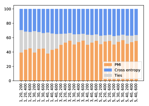
Figure 3: The average win rates of our PMI score and the test score benchmark. The orange bars represent the win rates or our PMI score, the blue bars represent the win rates of the benchmark (selection based on test score), and the gray bars represent the rates of ties. The label under the bar indicates $K,N_{T},M$.

As shown in Figure 2, our PMI score has a consistently higher win rate around 60%. Again, the win rate of the PMI score exhibits an upward trend with an increase in the number of candidate datasets $M$, suggesting that overfitting might be a contributing factor to the observed disparity and our PMI score could be more robust to overfitting.

References

- Blundell et al. (2015) Charles Blundell, Julien Cornebise, Koray Kavukcuoglu, and Daan Wierstra. Weight uncertainty in neural network. In International conference on machine learning, pages 1613–1622. PMLR, 2015.
- Chaudhuri et al. (2023) Kamalika Chaudhuri, Kartik Ahuja, Martin Arjovsky, and David Lopez-Paz. Why does throwing away data improve worst-group error? In Proceedings of the 40th International Conference on Machine Learning, ICML’23. JMLR.org, 2023.
- Chen et al. (2020) Yiling Chen, Yiheng Shen, and Shuran Zheng. Truthful data acquisition via peer prediction. Advances in Neural Information Processing Systems, 33:18194–18204, 2020.
- Feldman and Zhang (2020) Vitaly Feldman and Chiyuan Zhang. What neural networks memorize and why: Discovering the long tail via influence estimation. Advances in Neural Information Processing Systems, 33:2881–2891, 2020.
- Gelman et al. (1995) Andrew Gelman, John B Carlin, Hal S Stern, and Donald B Rubin. Bayesian data analysis. Chapman and Hall/CRC, 1995.
- Ghorbani and Zou (2019) Amirata Ghorbani and James Zou. Data shapley: Equitable valuation of data for machine learning. In International conference on machine learning, pages 2242–2251. PMLR, 2019.
- Gneiting and Raftery (2007) Tilmann Gneiting and Adrian E Raftery. Strictly proper scoring rules, prediction, and estimation. Journal of the American statistical Association, 102(477):359–378, 2007.
- Good (1952) I. J. Good. Rational decisions. Journal of the Royal Statistical Society. Series B (Methodological), 14(1):107–114, 1952. ISSN 00359246. URL http://www.jstor.org/stable/2984087.
- Jia et al. (2019) Ruoxi Jia, David Dao, Boxin Wang, Frances Ann Hubis, Nezihe Merve Gurel, Bo Li, Ce Zhang, Costas J Spanos, and Dawn Song. Efficient task-specific data valuation for nearest neighbor algorithms. arXiv preprint arXiv:1908.08619, 2019.
- Jiang et al. (2023) Kevin Fu Jiang, Weixin Liang, James Zou, and Yongchan Kwon. Opendataval: a unified benchmark for data valuation. arXiv preprint arXiv:2306.10577, 2023.
- Jurca and Faltings (2008) Radu Jurca and Boi Faltings. Incentives for expressing opinions in online polls. In Proceedings of the 9th ACM Conference on Electronic Commerce, pages 119–128, 2008.
- Koh and Liang (2017) Pang Wei Koh and Percy Liang. Understanding black-box predictions via influence functions. In International conference on machine learning, pages 1885–1894. PMLR, 2017.
- Kong and Schoenebeck (2018a) Yuqing Kong and Grant Schoenebeck. Equilibrium selection in information elicitation without verification via information monotonicity. In 9th Innovations in Theoretical Computer Science Conference, 2018a.
- Kong and Schoenebeck (2018b) Yuqing Kong and Grant Schoenebeck. Water from two rocks: Maximizing the mutual information. In Proceedings of the 2018 ACM Conference on Economics and Computation, EC ’18, page 177–194, New York, NY, USA, 2018b. Association for Computing Machinery. ISBN 9781450358293. doi: 10.1145/3219166.3219194. URL https://doi.org/10.1145/3219166.3219194.
- Kwon and Zou (2021) Yongchan Kwon and James Zou. Beta shapley: a unified and noise-reduced data valuation framework for machine learning. arXiv preprint arXiv:2110.14049, 2021.
- Kwon et al. (2023) Yongchan Kwon, Eric Wu, Kevin Wu, and James Zou. Datainf: Efficiently estimating data influence in lora-tuned llms and diffusion models. arXiv preprint arXiv:2310.00902, 2023.
- Miller et al. (2005) N. Miller, P. Resnick, and R. Zeckhauser. Eliciting informative feedback: The peer-prediction method. Management Science, pages 1359–1373, 2005.
- Murphy (2012) Kevin P Murphy. Machine learning: a probabilistic perspective. 2012.
- Nielsen (2019) Frank Nielsen. On the jensen–shannon symmetrization of distances relying on abstract means. Entropy, 21(5):485, 2019.
- Park et al. (2023) Sung Min Park, Kristian Georgiev, Andrew Ilyas, Guillaume Leclerc, and Aleksander Madry. Trak: Attributing model behavior at scale. arXiv preprint arXiv:2303.14186, 2023.
- Prelec (2004) D. Prelec. A Bayesian Truth Serum for subjective data. Science, 306(5695):462–466, 2004.
- Radanovic and Faltings (2013) Goran Radanovic and Boi Faltings. A robust bayesian truth serum for non-binary signals. In Proceedings of the 27th AAAI Conference on Artificial Intelligence (AAAI” 13), number EPFL-CONF-197486, pages 833–839, 2013.
- Radanovic and Faltings (2014) Goran Radanovic and Boi Faltings. Incentives for truthful information elicitation of continuous signals. In Proceedings of the 28th AAAI Conference on Artificial Intelligence (AAAI” 14), number EPFL-CONF-215878, pages 770–776, 2014.
- Schoenebeck and Yu (2020) Grant Schoenebeck and Fang-Yi Yu. Two strongly truthful mechanisms for three heterogeneous agents answering one question. In International Conference on Web and Internet Economics. Springer, 2020.
- Tierney (1994) Luke Tierney. Markov Chains for Exploring Posterior Distributions. The Annals of Statistics, 22(4):1701 – 1728, 1994. doi: 10.1214/aos/1176325750. URL https://doi.org/10.1214/aos/1176325750.
- Wand and Jones (1994) Matt P Wand and M Chris Jones. Kernel smoothing. CRC press, 1994.
- Wang and Jia (2022) Tianhao Wang and Ruoxi Jia. Data banzhaf: A data valuation framework with maximal robustness to learning stochasticity. arXiv preprint arXiv:2205.15466, 2022.
- Witkowski and Parkes (2012) Jens Witkowski and David C. Parkes. Peer prediction without a common prior. In Boi Faltings, Kevin Leyton-Brown, and Panos Ipeirotis, editors, Proceedings of the 13th ACM Conference on Electronic Commerce, EC 2012, Valencia, Spain, June 4-8, 2012, pages 964–981. ACM, 2012. doi: 10.1145/2229012.2229085. URL https://doi.org/10.1145/2229012.2229085.