Sensor-Based Distributionally Robust Control for Safe Robot Navigation in Dynamic Environments

Abstract

We introduce a novel method for safe mobile robot navigation in dynamic, unknown environments, utilizing onboard sensing to impose safety constraints without the need for accurate map reconstruction. Traditional methods typically rely on detailed map information to synthesize safe stabilizing controls for mobile robots, which can be computationally demanding and less effective, particularly in dynamic operational conditions. By leveraging recent advances in distributionally robust optimization, we develop a distributionally robust control barrier function (DR-CBF) constraint that directly processes range sensor data to impose safety constraints. Coupling this with a control Lyapunov function (CLF) for path tracking, we demonstrate that our CLF-DR-CBF control synthesis method achieves safe, efficient, and robust navigation in uncertain dynamic environments. We demonstrate the effectiveness of our approach in simulated and real autonomous robot navigation experiments, marking a substantial advancement in real-time safety guarantees for mobile robots.

1 Introduction

Ensuring real-time, high-frequency robot control with safety guarantees in dynamic and unstructured environments is crucial for the effective deployment of autonomous mobile robots. Khatib (1986) introduced the seminar artificial potential fields approach to enable collision avoidance for real-time control of mobile robots. This concept has inspired a wealth of research into the joint consideration of path planning and control, including techniques utilizing navigation functions (Rimon and Koditschek, 1992), dynamic windows (Fox et al., 1997), and velocity vector fields (De Lima and Pereira, 2013). A common thread in many of these works is the reliance on accurate map representations (Oleynikova et al., 2017; Herbert et al., 2017; Arslan and Koditschek, 2019; Axelrod et al., 2018; Li et al., 2023b) updated from onboard sensing to facilitate safe autonomous navigation. However, creating accurate maps in real-time with limited on-board computing resources is particularly challenging in dynamic environments. This work addresses this challenge by developing a distributionally robust formulation for safety constraints that directly processes range sensor data, avoiding the need for fast map updates and offering an adaptable solution for safe navigation in unstructured and dynamic environments.

Certificate functions have been introduced as powerful tools for asserting properties of dynamical systems, such as stability, safety, and robustness against uncertainties. Among these, Lyapunov functions (Artstein, 1983; Sontag, 1989) guarantee asymptotic stability for dynamical systems, and barrier functions (Prajna and Jadbabaie, 2004) certify forward invariance for desired safe sets. In recent years, control barrier functions (CBFs) have marked a significant advancement in encoding safety constraints for dynamical systems. In conjunction with control Lyapunov functions (CLFs) for stability guarantees, safe and stable controls can be synthesized online for control-affine nonlinear systems via quadratic programming (QP) (Ames et al., 2019). The CLF-CBF QP framework has become a mainstream approach for synthesizing reliable and safe controls in real-time for various robot systems (Desai and Ghaffari, 2022; Choi et al., 2023; Li et al., 2023a; Liu et al., 2023).

In this paper, we develop a novel approach to impose safety constraints for robot navigation in unknown and dynamic environments. Leveraging distributionally robust optimization (DRO), our method circumvents the requirement of a precisely known occupancy map and deals effectively with the uncertainty in direct range measurements. Conventionally, safe control synthesis with CBFs necessitates perfect knowledge of both the system model and the associated CBF (Ames et al., 2017). Although recent efforts have focused on estimating CBFs using sensory data like LiDAR and RGB-D in unknown environments (Long et al., 2022; Xiao et al., 2022; Abdi et al., 2023; Hamdipoor et al., 2023), these methods involve processing the sensor data to reconstruct the environment, a process that poses significant computational challenges in real-time robot applications.

Our approach addresses this bottleneck by enabling the evaluation of safety constraints at comparable frequency to control. Instead of estimating a CBF constraint and its uncertainty precisely, our formulation enables direct use of the measurements as noisy CBF samples defining a DRO safety constraint. Our formulation enhances the robustness of safe control synthesis in complex real-world scenarios (e.g., thin chair legs, netting in Fig. 1), where constructing accurate CBFs from sensor measurements is particularly challenging. This advancement represents a critical step in ensuring safer and more reliable autonomous robot navigation in dynamically changing and challenging environments.

The main contributions of this paper are as follows.

• We formulate a novel distributionally robust control barrier function (DR-CBF) constraint directly using onboard range measurements to synthesize safe controls that circumvent the need for fast, precise map updates in dynamic environments.

• Coupling the safety constraint with a control Lyapunov function (CLF) for path tracking, we introduce a CLF-DR-CBF quadratic program for synthesizing safe stabilizing controls for nonlinear control-affine systems.

• We validate the safety, efficiency, and robustness of our approach in simulated and real experiments of autonomous differential-drive robot navigation in unknown and dynamic environments.

• We provide an open-source implementation of our proposed CLF-DR-CBF controller.

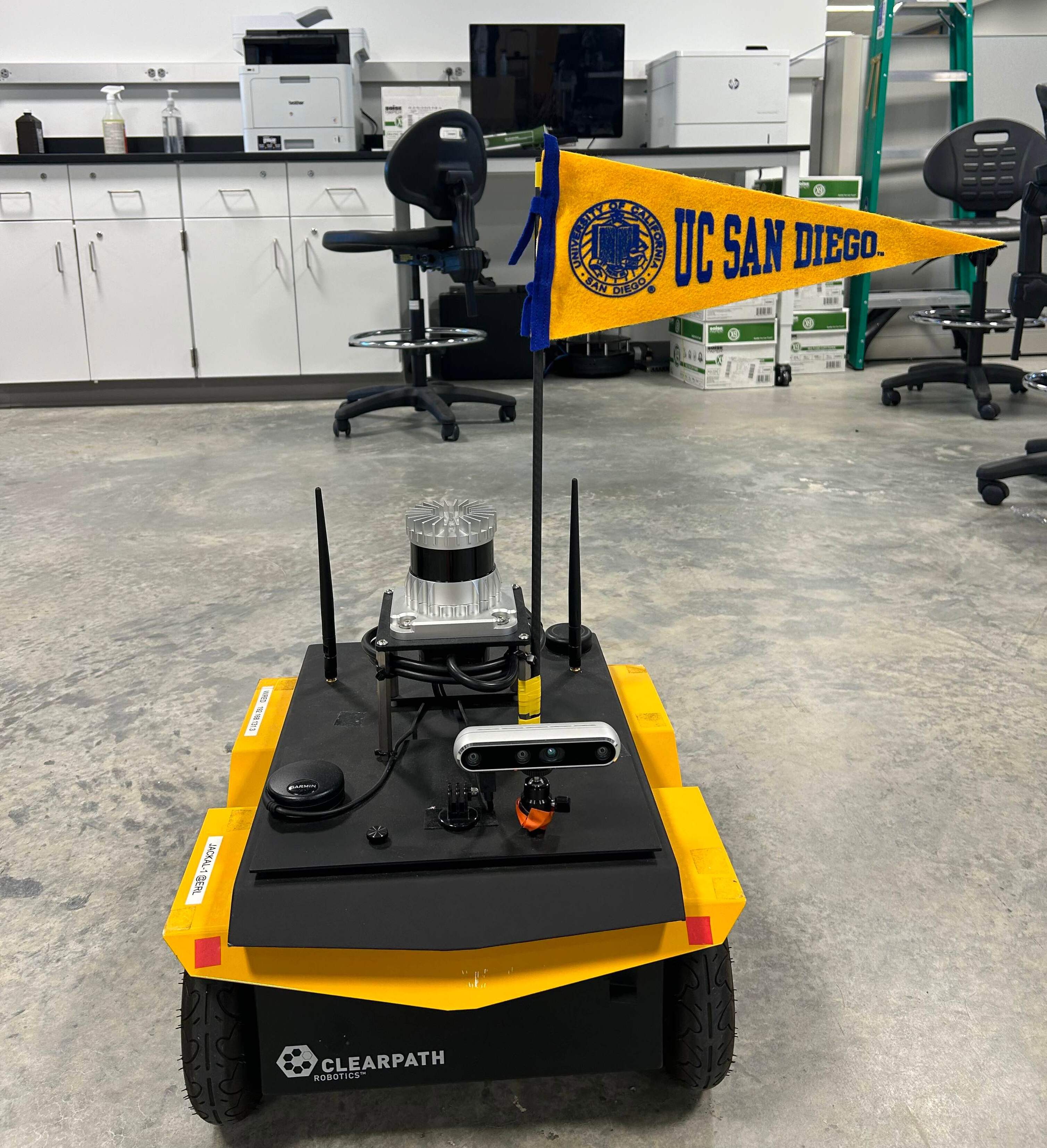
(a) Indoor environment

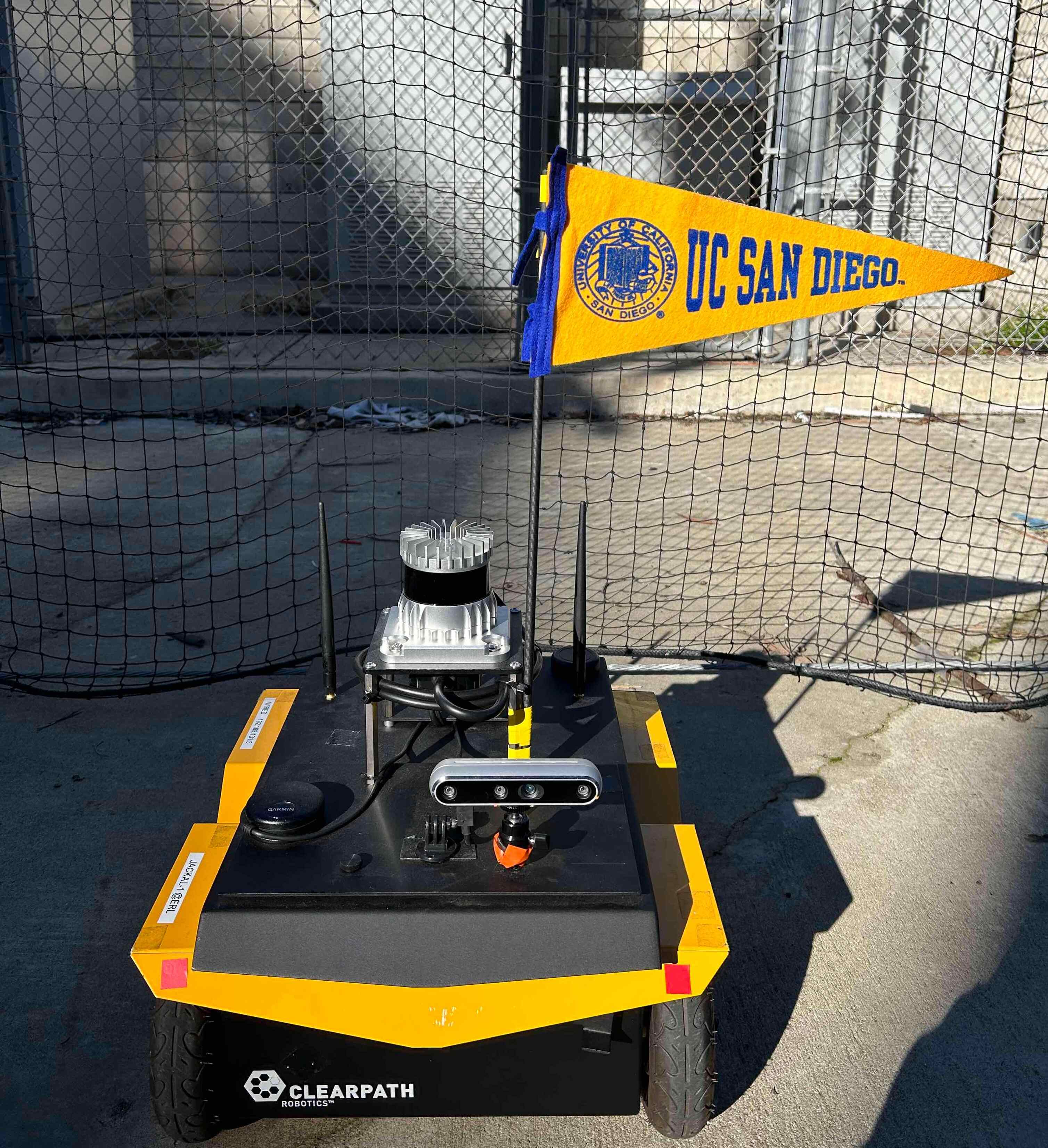
(b) Outdoor environment

Figure 1: ClearPath Jackal robot equipped with a LiDAR sensor navigating in unknown indoor and outdoor environments.

2 Related Work

This section reviews related work on dynamic obstacle avoidance, distributionally robust optimization, and CLF-CBF techniques for safe stabilizing control.

Dynamic obstacle avoidance. Robot motion planning algorithms have a rich history, dating back to the 1950s with the introduction of Dijkstra algorithm (Dijkstra, 1959) and $A^{*}$ (Hart et al., 1968) for search-based planning in known environments. Since then, a substantial amount of research has been dedicated to algorithms for collision-free path planning and low-level control that allow robots to follow the planned paths (Lozano-Perez, 1983; Brooks, 1983). A significant contribution was made by Khatib (1986), who introduced artificial potential fields to enable collision avoidance during not only the motion planning stage but also the real-time control of a mobile robot. The formulation was extended to a virtual force field (Borenstein et al., 1991), facilitating safe navigation in uncertain environments. Later, Rimon and Koditschek (1992) developed navigation functions, a particular form of artificial potential functions, which simultaneously ensure collision avoidance and stabilization to a goal configuration. The dynamic window concept was introduced by Fox et al. (1997) to handle dynamic obstacles by proactively filtering out unsafe control actions. Later, this idea was combined with a global desired velocity vector field to allow safe navigation in De Lima and Pereira (2013). More recently, Herbert et al. (2017) developed FaSTrack, a modular framework that utilizes Hamilton-Jacobi reachability analysis and a game-theoretic formulation between planner and controller to enable rapid and safe robot navigation in complex environments. Majd et al. (2021) integrate time-based rapidly-exploring random trees (RRTs) with CBFs to enable safe navigation in dynamic environments densely populated by pedestrians. Recent advancements in reinforcement learning have also led to real-time solutions for obstacle avoidance and navigation (Pfeiffer et al., 2018; Everett et al., 2021; Chen et al., 2022), typically framing the problem as a partially observable Markov decision processe to facilitate model-free learning of control policies.

While these methods show promise, most require knowledge or estimation of environment geometry, typically through topological (Dudek et al., 1978) and metric (Chatila and Laumond, 1985; Borenstein et al., 1991) map representations. The signed distance function (SDF) has emerged as a particularly valuable tool in this regard (Oleynikova et al., 2017; Han et al., 2019; Wu et al., 2023), offering distance and gradient information for safe control and navigation. However, constructing real-time occupancy or SDF estimates is challenging with onboard sensing and limited computing resources, particularly in complex and dynamic environments.

Distributionally robust optimization. Distributionally Robust Optimization (DRO) considers parameter uncertainty in optimization problems, and is particularly effective when dealing with a limited number of uncertainty samples. This method compensates for the potential discrepancy between empirical and true uncertainty distributions, utilizing uncertainty descriptors like moment ambiguity sets (Van Parys et al., 2016), Kullback–Leibler ambiguity sets (Jiang and Guan, 2016), and Wasserstein ambiguity sets (Esfahani and Kuhn, 2018; Xie, 2021). The DRO framework has been increasingly utilized for its robust performance guarantees against distributional uncertainty in control (Boskos et al., 2024; Mestres et al., 2024; Long et al., 2023a; Chriat and Sun, 2023) and robotics (Ren and Majumdar, 2022; Coulson et al., 2021) applications.

Lathrop et al. (2021) proposed the Wasserstein safe RRT, a path planning algorithm offering finite-sample probabilistic safety guarantees in uncertain non-convex obstacle environments. A DRO-based approach was introduced by Ren and Majumdar (2022) to enhance policy robustness by iteratively training with adversarial environments generated through a learned generative model. Long et al. (2023b) proposed a DRO formulation for safe stabilizing control under model uncertainty, assuming that nominal safety and stability certificates are provided. Hakobyan and Yang (2022) introduced a distributionally robust risk map as a safety specification tool for mobile robots, effectively reformulating the optimization problem over an infinite-dimensional probability distribution space into a tractable semidefinite program. Boskos et al. (2023) proposed a distributionally robust coverage control algorithm for a team of robots to optimally deploy in a spatial region with an unknown event probability density. A Wasserstein tube MPC is presented in Aolaritei et al. (2023) for stochastic systems, which utilizes Wasserstein ambiguity sets to construct tubes around nominal trajectories, enhancing robustness and efficiency with limited noise samples available. Ramesh et al. (2023) introduced a model-based approach that utilizes the maximum variance reduction algorithm to efficiently learn nominal transition dynamics and near-optimal distributionally robust policies for stochastic systems.

Safe stabilizing control. Quadratic programming that integrates CLF and CBF constraints presents a certifiable and efficient framework for synthesizing safe stabilizing controls in a variety of tasks. These tasks span from multi-robot safe navigation (Zhang et al., 2023), to safe locomotion of legged robots (Grandia et al., 2021), and to safe humanoid operation (Khazoom et al., 2022). Despite the efficiency of the CLF-CBF QP in synthesizing safe stabilizing controls, it typically relies on perfect knowledge of system dynamics, state estimates, and barrier function constraints. However, in many robotics applications, various sources of uncertainty can significantly impact performance and reliability. Some recent studies have begun to explore this area, to address uncertainty in system dynamics (Dhiman et al., 2023; Emam et al., 2022), state estimates (Daş and Murray, 2022; Wang and Xu, 2023), and barrier function constraints (Long et al., 2021; Hamdipoor et al., 2023). These approaches typically utilize robust and probabilistic models to integrate uncertainty into the QP formulation, leading to convex reformulations that enhance robustness.

Particularly in safe robot navigation, a robot might need to estimate barrier functions based on its (noisy) observations. Long et al. (2021) introduced an incremental online learning approach for estimating the barrier function from LiDAR data and proposed a robust reformulation of the CLF-CBF QP by incorporating estimation errors. Dawson et al. (2022) developed an approach to learn observation-space CBFs utilizing distance data and proposed a two-mode hybrid controller to avoid deadlocks in navigation. A reactive planning algorithm was presented in Liu et al. (2023) for the safe operation of a bipedal robot with multiple obstacles, utilizing a single differentiable CBF derived from LiDAR point clouds. Abdi et al. (2023) proposed a method for learning vision-based CBF from RGB-D images with pre-training, enabling safe navigation of autonomous vehicles in unseen environments. By effectively decomposing and predicting the spatial interactions of multiple obstacles, Yu et al. (2023) proposed compositional learning of sequential CBFs, enabling obstacle avoidance in dense dynamic environments. Keyumarsi et al. (2024) introduced an efficient Gaussian Process-based method for synthesizing CBFs from LiDAR data, showcasing its effectiveness in a turtlebot navigation task. Zhang et al. (2024) introduced an efficient LiDAR-based framework for goal-seeking and exploration of mobile robots in dynamic environments, utilizing minimum bounding ellipses to represent obstacles and Kalman filters to estimate their velocities.

A related line of research to our work is the application of conformal prediction in robot navigation tasks. Conformal prediction (Shafer and Vovk, 2008; Zhao et al., 2024) is a statistical tool for uncertainty quantification that provides valid prediction regions with a user-specified risk tolerance, making it particularly useful for ensuring safety in dynamic environments. Several recent works have explored the integration of conformal prediction into motion planning and control frameworks. Lindemann et al. (2023) used conformal prediction to obtain prediction regions for a model predictive controller. Yang et al. (2023) employed conformal prediction to quantify state estimation uncertainty and design a robust CBF controller based on the estimated uncertainty. An adaptive conformal prediction algorithm was developed by Dixit et al. (2023) to dynamically quantify prediction uncertainty and plan probabilistically safe paths around dynamic agents.

3 Background

This section introduces our notation and offers a brief review of CLF-CBF QP.

3.1 Notation

The sets of real, non-negative real, and natural numbers are denoted by $\mathbb{R}$, $\mathbb{R}_{\geq 0}$, and $\mathbb{N}$, respectively. For $N\in\mathbb{N}$, we write $[N]:=\{1,2,\dots N\}$. We denote the distribution and expectation of a random variable $Y$ by $\mathbb{P}$ and $\mathbb{E}_{\mathbb{P}}(Y)$, respectively. We use $\boldsymbol{0}$ and $\boldsymbol{1}$ to denote the vector with all entries equal to $0$ and $1$, respectively. For a scalar $x$, we define $(x)_{+}:=\max(x,0)$. We denote by $\mathbf{I}_{n}\in\mathbb{R}^{n\times n}$ the identity matrix. For a scalar $x$ and $y$, we use $\text{atan2}(y,x)$ to denote the angle between the positive $x$-axis and the point $(x,y)$ in radians. The interior and boundary of a set ${\cal C}\subset\mathbb{R}^{n}$ are denoted by $\text{Int}({\cal C})$ and $\partial{\cal C}$. For a vector $\mathbf{x}$, the notation $|\mathbf{x}|$ represents its element-wise absolute value, while $\|\mathbf{x}\|_{1}$, $\|\mathbf{x}\|$, and $\|\mathbf{x}\|_{\infty}$ denote its $L_{1}$, $L_{2}$, and $L_{\infty}$ norms, respectively. The gradient of a differentiable function $V:\mathbb{R}^{n}\rightarrow\mathbb{R}$ is denoted by $\nabla V$, while its Lie derivative along a vector field $\mathbf{f}:\mathbb{R}^{n}\rightarrow\mathbb{R}^{n}$ is ${\cal L}_{\mathbf{f}}V=\nabla V^{\top}\mathbf{f}$. A continuous function $\alpha:[0,a)\rightarrow[0,\infty)$ is of class ${\cal K}$ if it is strictly increasing and $\alpha(0)=0$. A continuous function $\alpha:\mathbb{R}\rightarrow\mathbb{R}$ is of extended class ${\cal K}_{\infty}$ if it is strictly increasing, $\alpha(0)=0$, and $\lim_{r\rightarrow\infty}\alpha(r)=\infty$. The special orthogonal group of dimension $p$ is denoted by $SO(p)$, which is defined as the set of all $p\times p$ orthogonal matrices with determinant equal to 1: $SO(p)=\{\mathbf{R}\in\mathbb{R}^{p\times p}\mid\mathbf{R}^{\top}\mathbf{R}=\mathbf{I}_{p},\det(\mathbf{R})=1\}$.

3.2 CLF-CBF Quadratic Program

Consider a non-linear control-affine system,

$$\dot{\mathbf{x}}=\mathbf{f}(\mathbf{x})+\mathbf{g}(\mathbf{x})\mathbf{u}=[\mathbf{f}(\mathbf{x})\;\mathbf{g}(\mathbf{x})]\begin{bmatrix}1\\ \mathbf{u}\end{bmatrix}=:\mathbf{F}(\mathbf{x})\underline{\mathbf{u}},$$ (1)

where $\mathbf{x}\in{\cal X}\subseteq\mathbb{R}^{n}$ is the state, $\mathbf{u}\in\mathbb{R}^{m}$ is the control input, and $\mathbf{f}:\mathbb{R}^{n}\rightarrow\mathbb{R}^{n}$ and $\mathbf{g}:\mathbb{R}^{n}\rightarrow\mathbb{R}^{n\times m}$ are locally Lipschitz continuous functions.

The notion of a control Lyapunov function (CLF) (Artstein, 1983; Sontag, 1989) plays a key role in certifying the stabilizability of control-affine systems.

Definition 3.1.

A continuously differentiable function $V:\mathbb{R}^{n}\rightarrow\mathbb{R}$ is a control Lyapunov function (CLF) on ${\cal X}$ for system (1) if $V(\mathbf{x})>0$, $\forall\mathbf{x}\in{\cal X}\setminus\{\boldsymbol{0}\}$, $V(\boldsymbol{0})=0$, and

$$\inf_{\mathbf{u}\in\mathbb{R}^{m}}\text{CLC}(\mathbf{x},\mathbf{u})\leq 0,\quad\forall\mathbf{x}\in{\cal X},$$ (2)

where $\text{CLC}(\mathbf{x},\mathbf{u}):=\mathcal{L}_{\mathbf{f}}V(\mathbf{x})+\mathcal{L}_{\mathbf{g}}V(\mathbf{x})\mathbf{u}+\alpha_{V}(V(\mathbf{x}))$ is the control Lyapunov constraint (CLC) defined for some class ${\cal K}$ function $\alpha_{V}$.

To facilitate safe control synthesis, we consider a time-varying set ${\cal C}(t)$ defined as the zero superlevel set of a continuously differentiable function $h:{\cal X}\times\mathbb{R}_{\geq 0}\rightarrow\mathbb{R}$:

$${\cal C}(t):=\{\mathbf{x}\in{\cal X}:h(\mathbf{x},t)\geq 0\}.$$ (3)

Safety of the system (1) can then be ensured by keeping the state $\mathbf{x}$ within the safe set ${\cal C}(t)$.

Definition 3.2.

A continuously differentiable function $h:\mathbb{R}^{n}\times\mathbb{R}_{\geq 0}\rightarrow{\mathbb{R}}$ is a time-varying control barrier function (TV-CBF) on $\mathcal{X}\subseteq\mathbb{R}^{n}$ for (1) if there exists an extended class $\mathcal{K}_{\infty}$ function $\alpha_{h}$ with:

$$\sup_{\mathbf{u}\in\mathcal{U}}\text{CBC}(\mathbf{x},\mathbf{u},t)\geq 0,\quad\forall\;(\mathbf{x},t)\in{\cal X}\times\mathbb{R}_{\geq 0},$$ (4)

where the control barrier constraint (CBC) is:

$$\text{CBC}(\mathbf{x},\mathbf{u},t):=\dot{h}(\mathbf{x},t)+\alpha_{h}(h(\mathbf{x},t))$$ (5)

$$=\mathcal{L}_{\mathbf{f}}h(\mathbf{x},t)+\mathcal{L}_{\mathbf{g}}h(\mathbf{x},t)\mathbf{u}+\frac{\partial h(\mathbf{x},t)}{\partial t}+\alpha_{h}(h(\mathbf{x},t)).$$

Definition 3.2 allows us to consider the set of control values $K_{\text{CBF}}(\mathbf{x},t):=\left\{\mathbf{u}\in\mathbb{R}^{m}:\text{CBC}(\mathbf{x},\mathbf{u},t)\geq 0\right\}$ that render the set ${\cal C}(t)$ forward invariant.

Definition 3.3.

Let $t_{0}$ be a fixed initial time. A time-varying set ${\cal C}(t)$ is said to be forward invariant under control law $\mathbf{u}:[t_{0},\infty)\rightarrow\mathbb{R}^{m}$ if, for any initial state $\mathbf{x}_{0}\in{\cal C}(t_{0})$, there exists a unique maximal solution $\mathbf{x}:[t_{0},t_{1})\rightarrow\mathbb{R}^{n}$ to the system dynamics in (1) with $\mathbf{x}(t_{0})=\mathbf{x}_{0}$, such that $\mathbf{x}(t)\in{\cal C}(t)$ for all $t\in[t_{0},t_{1})$.

Suppose we are given a baseline feedback controller $\mathbf{u}=\mathbf{k}(\mathbf{x})$ and we aim to ensure the safety and stability of the control-affine system (1). By observing that both the stability and safety constraints in (2), (4) are affine in the control input $\mathbf{u}$, a quadratic program (Ames et al., 2017) can be formulated to synthesize a safe stabilizing controller:

$$(\mathbf{u}(\mathbf{x},t),\delta)\in \operatorname*{arg\,min}_{\mathbf{u}\in\mathbb{R}^{m},\delta\in\mathbb{R}}\|\mathbf{u}-\mathbf{k}(\mathbf{x})\|^{2}+\lambda\delta^{2},$$ (6)

$$\mathrm{s.t.} \text{CLC}(\mathbf{x},\mathbf{u})\leq\delta,\text{CBC}(\mathbf{x},\mathbf{u},t)\geq 0,$$

where $\delta$ denotes a slack variable that relaxes the CLF constraint to ensure feasibility of the QP, controlled by the scaling factor $\lambda>0$. As discussed in Ames et al. (2017); Mestres et al. (2023), if the CBF $h$ has relative degree of $1$ with respect to the system dynamics in (1), the controller in (6) is Lipschitz continuous in $\mathbf{x}$ and piecewise continuous in $t$. This guarantees unique solutions for the closed-loop system, ensuring the safe set ${\cal C}(t)$ remains forward invariant.

4 Problem Formulation

We consider a mobile robot that relies on noisy range measurements to traverse an unknown dynamic environment towards a desired goal. The environment contains both static and dynamic obstacles. We define the obstacle space as a closed set ${\cal O}(t)\subset\mathbb{R}^{p}$, and the free space as an open set ${\cal F}(t)=\mathbb{R}^{p}\setminus{\cal O}(t)$.

The robot’s motion is governed by control-affine dynamics as in (1). Let $\phi:{\cal X}\rightarrow\mathbb{R}^{p}$ project the robot state $\mathbf{x}$ to its position $\phi(\mathbf{x})\in\mathbb{R}^{p}$, and denote the robot’s body as ${\cal B}(\mathbf{x})\subset\mathbb{R}^{p}$.

The robot is equipped with a range sensor (e.g., LiDAR) mounted at a fixed position $\mathbf{q}_{s}\in\mathbb{R}^{p}$ and orientation $\mathbf{R}_{s}\in SO(p)$ in the robot’s body frame. This sensor generates noisy distance measurements $\boldsymbol{\eta}(\mathbf{q}_{s},\mathbf{R}_{s})=[\eta_{1}(\mathbf{q}_{s},\mathbf{R}_{s}),...,\eta_{K}(\mathbf{q}_{s},\mathbf{R}_{s})]^{\top}\in[\eta_{\text{min}},\eta_{\text{max}}]^{K}$, where $K$ denotes the number of rays per sensor observation and $\eta_{\text{min}},\eta_{\text{max}}$ denote the sensor’s minimum and maximum range, respectively.

Problem.

Consider a mobile robot with dynamics as in (1), equipped with a range sensor, operating in an unknown dynamic environment. Design a control policy that safely and efficiently drives the robot to a desired goal position $\mathbf{q}_{G}\in\mathbb{R}^{p}$, while ensuring that the robot’s body satisfies ${\cal B}(\mathbf{x}(t))\subset{\cal F}(t)$ for all $t\geq 0$, despite sensing and environment uncertainty.

5 System Overview

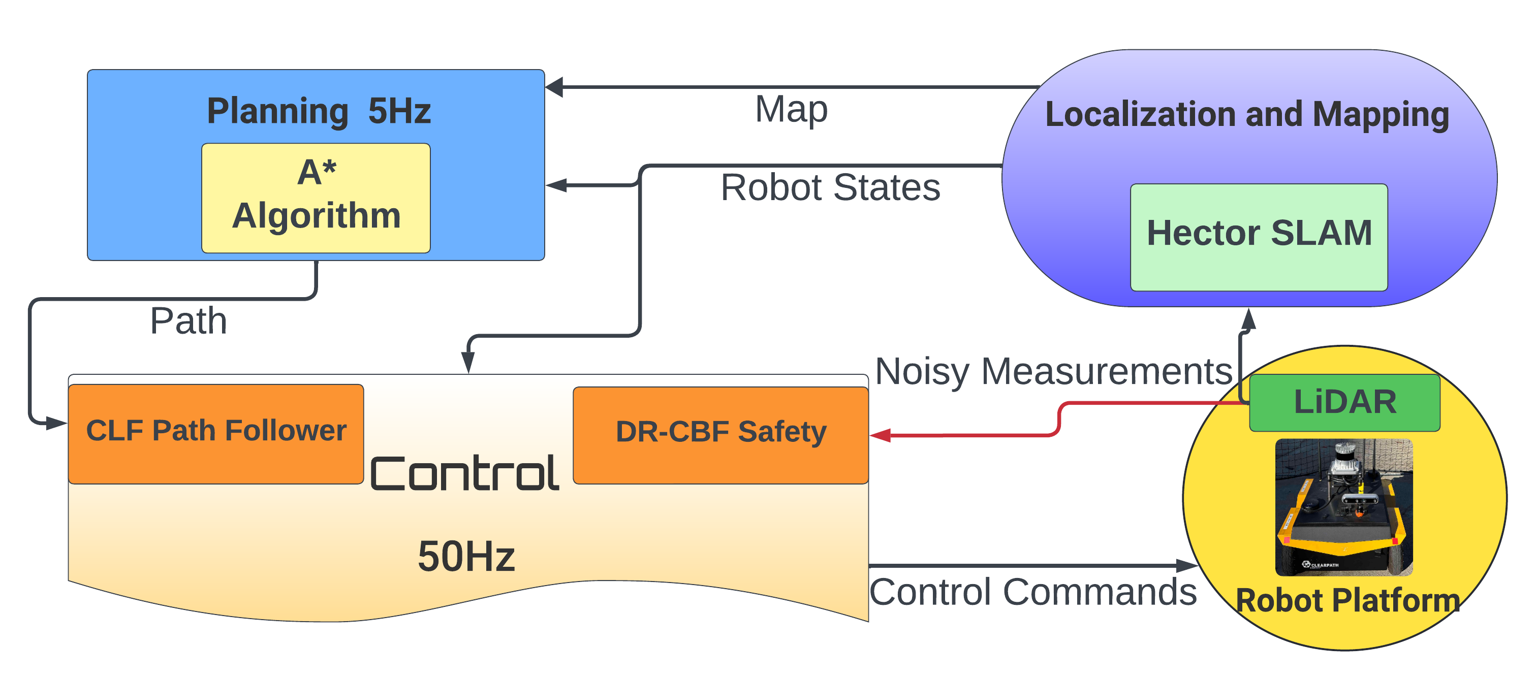
Figure 2: Overview of our approach for safe robot navigation in unknown dynamic environments. The system consists of three main components: (1) localization and mapping, (2) path planning, and (3) control. The contribution of this work lies in the control component, where a novel distributionally robust control barrier function is used to ensure safety in real-time, directly utilizing sensor data, and a control Lyapunov function is used to navigate cluttered and dynamic environments.

This section describes the methods we use for localization and mapping, path planning, and control to enable safe robot navigation. Our contribution is the control method, which includes a distributionally robust time-varying control barrier function to guarantee safety in dynamic environments, presented in Sec. 6, and a control Lyapunov function for stable path-following control introduced in Sec. 7. While our control method is applicable to general control-affine systems (1) under certain assumptions, our experiments focus on a wheeled differential-drive robot.

We consider a robot with state $\mathbf{x}:=[x,y,\theta]^{\top}\in{\cal X}\subseteq\mathbb{R}^{2}\times[-\pi,\pi)$, input $\mathbf{u}:=[v,\omega]^{\top}\in\mathbb{R}^{2}$, and dynamics:

$$\dot{\mathbf{x}}=\left[\begin{matrix}\cos(\theta)&0\\ \sin(\theta)&0\\ 0&1\end{matrix}\right]\left[\begin{matrix}v\\ \omega\end{matrix}\right].$$ (7)

The function $\phi:{\cal X}\rightarrow\mathbb{R}^{2}$ that projects the robot state $\mathbf{x}$ to its position is $\phi(\mathbf{x})=\phi([x,y,\theta]^{\top})=[x,y]^{\top}$. Fig. 2 presents an overview of the robot autonomy components, which are described next.

Localization and Mapping. The robot is equipped with a LiDAR scanner and uses the Hector SLAM algorithm (Kohlbrecher et al., 2011) to estimate its pose and build an occupancy map of the environment. We emphasize that the accuracy and detail of the occupancy map may not be sufficient to ensure safe navigation in a dynamic environment. We use the map for high-level path planning and employ a low-level controller to guarantee safe tracking using CLF and CBF techniques.

Path Planning. We use the $A^{*}$ planning algorithm (Hart et al., 1968) to generate a path $\gamma:[0,1]\mapsto\mathbb{R}^{p}$ from the robot’s current position $\phi(\mathbf{x})\in\mathbb{R}^{p}$ to the goal $\mathbf{q}_{G}\in\mathbb{R}^{p}$. The path $\gamma(s)$ is parametrized by a scalar $s\in[0,1]$ such that $\gamma(0)=\phi(\mathbf{x})$ and $\gamma(1)=\mathbf{q}_{G}$. As the robot navigates through the environment, the map is continuously updated by the SLAM algorithm and the path is continuously replanned to adapt to changes in the map.

Control. Our control approach simultaneously guarantees the robot’s adherence to the planned path $\gamma$ and its safety from collisions in the dynamically changing environment. In Sec. 6, we develop a distributionally robust CBF that uses noisy distance measurements directly to guarantee safety with respect to dynamic obstacles. In Sec. 7, we develop a CLF to track the path $\gamma$ with stability guarantees.

6 Distributionally Robust Safe Control

In this section, we present a distributionally robust control barrier function (DR-CBF) formulation that enables real-time safety guarantees in cluttered and dynamic environments by utilizing sensor data directly. This formulation is applicable to general control-affine systems (1), as introduced in Sec. 4.

We consider a CBF $h(\mathbf{x},t)$ such that its superlevel set ${\cal C}(t)$ in (3) is a subset of $\{\mathbf{x}\in{\cal X}\mid{\cal B}(\mathbf{x}(t))\subset{\cal F}(t)\}$. To develop the DR-CBF formulation, we make the following assumption on the unknown CBF.

Assumption 6.1.

The CBF $h(\mathbf{x},t)$ satisfies the following assumptions:

1. $h(\mathbf{x},t)$ has a uniform relative degree of 1 with respect to the system dynamics (1), i.e., the time derivative of $h(\mathbf{x},t)$ along (1) depends explicitly on the control input $\mathbf{u}$;

2. the condition in (5) is satisfied for a linear ${\cal K}_{\infty}$ function $\alpha_{h}$, i.e., $\alpha_{h}(z)=az$ for $a\in\mathbb{R}_{>0}$.

Under Assumption 6.1, we can write the control barrier constraint associated with $h(\mathbf{x},t)$ as:

$$\text{CBC}(\mathbf{x},\mathbf{u},t)\!=\![\nabla_{\mathbf{x}}h(\mathbf{x},t)]^{\top}\mathbf{F}(\mathbf{x})\underline{\mathbf{u}}+\frac{\partial h(\mathbf{x},t)}{\partial t}+ah(\mathbf{x},t)$$

$$=[a\;\;\mathbf{F}(\mathbf{x})\underline{\mathbf{u}}\;\;1]^{\top}[h(\mathbf{x},t)\;\;\nabla_{\mathbf{x}}h(\mathbf{x},t)\;\;\frac{\partial h(\mathbf{x},t)}{\partial t}]\geq 0.\!\!$$ (8)

For each $(\mathbf{x},t)\in{\cal X}\times\mathbb{R}$, we consider the vector $\boldsymbol{\xi}(\mathbf{x},t):=[h(\mathbf{x},t),\nabla_{\mathbf{x}}h(\mathbf{x},t),\frac{\partial h(\mathbf{x},t)}{\partial t}]\in\mathbb{R}^{n+2}$. Since the environment is unknown and the sensor measurements are noisy, $\boldsymbol{\xi}$ cannot be determined exactly. Our objective is to guarantee the satisfaction of constraint (6) despite the uncertainty in $\boldsymbol{\xi}$. To achieve this, we employ distributionally robust optimization techniques, which handle the uncertainty in (6). Before delving into the details of our approach, we review preliminaries of chance constraints and distributionally robust optimization.

6.1 Chance Constraints and Distributionally Robust Optimization

Consider a random vector $\boldsymbol{\xi}$ with (unknown) distribution $\mathbb{P}^{*}$ supported on the set $\Xi\subseteq\mathbb{R}^{k}$. Let $G:\mathbb{R}^{m}\times\Xi\to\mathbb{R}$ define an inequality constraint $G(\mathbf{u},\boldsymbol{\xi})\leq 0$ (e.g., the CBC in (6)). Consider, then, the chance-constrained program,

$$\min_{\mathbf{u}\in\mathbb{R}^{m}}c(\mathbf{u}),$$ (9)

$$\mathrm{s.t.} \mathbb{P}^{*}(G(\mathbf{u},\boldsymbol{\xi})\leq 0)\geq 1-\epsilon,$$

where $c:\mathbb{R}^{m}\mapsto\mathbb{R}$ is a convex objective function (e.g., the objective function in (6)) and $\epsilon\in(0,1)$ denotes a user-specified risk tolerance. Generally, the chance constraint in (LABEL:eq:_ccp) leads to a non-convex feasible set. To address this, Nemirovski and Shapiro (2006) propose a convex conditional value-at-risk (CVaR) approximation of the original chance constraint.

Value-at-risk (VaR) at confidence level $1-\epsilon$ for $\epsilon\in(0,1)$ is defined as $\text{VaR}_{1-\epsilon}^{\mathbb{P}_{q}}(Q):=\inf_{s\in\mathbb{R}}\{s\;|\;\mathbb{P}_{q}(Q\leq s)\geq 1-\epsilon\}$ for a random variable $Q$ with distribution $\mathbb{P}_{q}$. As VaR does not provide information about the right tail of the distribution and leads to intractable optimization in general, one can employ CVaR instead, defined as $\text{CVaR}_{1-\epsilon}^{\mathbb{P}_{q}}(Q)=\mathbb{E}_{\mathbb{P}_{q}}[Q\;|\;Q\geq\text{VaR}_{1-\epsilon}^{\mathbb{P}_{q}}(Q)]$. The resulting constraint

$$\text{CVaR}_{1-\epsilon}^{\mathbb{P}^{*}}(G(\mathbf{u},\boldsymbol{\xi}))\leq 0$$ (10)

creates a convex feasible set, which is a subset of the feasible set in the original chance-constrained problem (LABEL:eq:_ccp). Additionally, CVaR can be written as the following convex program (Rockafellar and Uryasev, 2000):

$$\text{CVaR}_{1-\epsilon}^{\mathbb{P}^{*}}(G(\mathbf{u},\boldsymbol{\xi})):=\inf_{s\in\mathbb{R}}[\epsilon^{-1}\mathbb{E}_{\mathbb{P}^{*}}[(G(\mathbf{u},\boldsymbol{\xi})+s)_{+}]-s].$$ (11)

The formulations in (LABEL:eq:_ccp) and (10) require knowledge of $\mathbb{P}^{*}$ to be utilized. However, in many robotics applications, usually only samples of the uncertainty $\boldsymbol{\xi}$ are available (e.g., obtained from LiDAR distance measurements). This motivates us to consider distributionally robust formulations (Esfahani and Kuhn, 2018; Xie, 2021).

Assuming finitely many samples $\{\boldsymbol{\xi}_{i}\}_{i\in[N]}$ from the true distribution of $\mathbb{P}^{*}$ are available, we first describe a way of constructing an ambiguity set of distributions that agree with the empirical distribution. Let ${\cal P}_{p}(\Xi)\subseteq{\cal P}(\Xi)$ be the set of Borel probability measures with finite $p$-th moment with $p\geq 1$. The $p$-Wasserstein distance between two probability measures $\mu$, $\nu$ in ${\cal P}_{p}(\Xi)$ is defined as:

$$W_{p}(\mu,\nu):=\left(\inf_{\beta\in\mathbb{Q}(\mu,\nu)}\left[\int_{\Xi\times\Xi}\eta(\boldsymbol{\xi},\boldsymbol{\xi}^{\prime})^{p}\text{d}\beta(\boldsymbol{\xi},\boldsymbol{\xi}^{\prime})\right]\right)^{\frac{1}{p}},$$ (12)

where $\mathbb{Q}(\mu,\nu)$ denotes the collection of all measures on $\Xi\times\Xi$ with marginals $\mu$ and $\nu$ on the first and second factors, and $\eta$ denotes the metric in the space $\Xi$. Throughout the paper, we take $\eta(\boldsymbol{\xi},\boldsymbol{\xi}^{\prime})=\|\boldsymbol{\xi}-\boldsymbol{\xi}^{\prime}\|_{1}$ and consider the ambiguity set corresponding to the $1$-Wasserstein distance. We denote by $\mathbb{P}_{N}:=\frac{1}{N}\sum_{i=1}^{N}\delta_{\boldsymbol{\xi}_{i}}$ the discrete empirical distribution of the available samples $\{\boldsymbol{\xi}_{i}\}_{i\in[N]}$, and define an ambiguity set, ${\cal M}_{N}^{r}:=\{\mu\in{\cal P}_{p}(\Xi)\;|\;W_{p}(\mu,\mathbb{P}_{N})\leq r\}$, as a ball of distributions with radius $r$ centered at $\mathbb{P}_{N}$.

Remark 6.2.

(Choice of Wasserstein ball radius): There is a connection between the sample size $N$ and the Wasserstein radius $r$ for constructing the ambiguity set ${\cal M}_{N}^{r}$. A distribution $\mathbb{P}$ is light-tailed if there exists an exponent $\rho$ such that $A:=\mathbb{E}_{\mathbb{P}}[\exp{\left\lVert\boldsymbol{\xi}\right\rVert^{\rho}}]=\int_{\Xi}\exp{\left\lVert\boldsymbol{\xi}\right\rVert^{\rho}}\mathbb{P}(d\boldsymbol{\xi})<\infty$. If the true distribution $\mathbb{P}^{*}$ is light-tailed, the choice of $r=r_{N}(\bar{\epsilon})$ given in Esfahani and Kuhn (2018, Theorem 3.5),

$$r_{N}(\bar{\epsilon})=\begin{cases}(\frac{\log(c_{1}\bar{\epsilon}^{-1})}{c_{2}N})^{\frac{1}{\max\{k,2\}}}\quad&\text{if}\ N\geq\frac{\log(c_{1}\bar{\epsilon}^{-1})}{c_{2}},\\ (\frac{\log(c_{1}\bar{\epsilon}^{-1})}{c_{2}N})^{\frac{1}{\rho}}\quad&\text{else},\end{cases}$$ (13)

where $c_{1},c_{2}$ are positive constants that depend on $\rho,A$ and $k$, ensures that the ambiguity ball ${\cal M}_{N}^{r_{N}(\bar{\epsilon})}$ contains $\mathbb{P}^{*}$ with probability at least $1-\bar{\epsilon}$.  $\bullet$

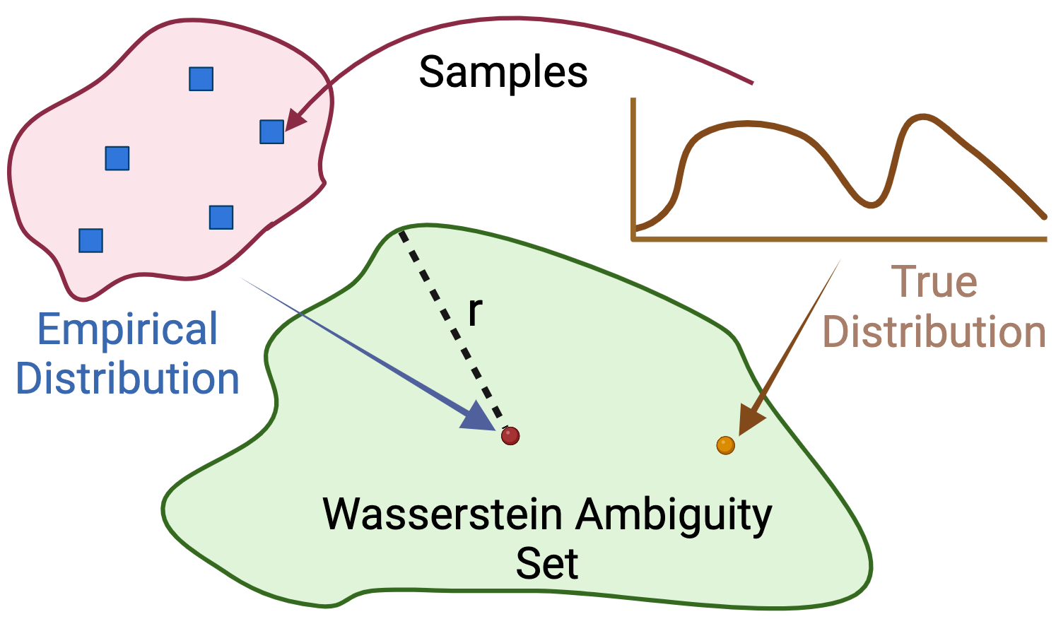
Figure 3: Wasserstein ambiguity set illustration. The figure shows the relationship between the samples, empirical distribution, true distribution, and the Wasserstein ambiguity set. The blue squares represent the available samples from the true distribution (yellow dot), which form the empirical distribution (red dot). The Wasserstein ambiguity set (green region) is constructed as a ball of distributions centered at the empirical distribution, with a radius $r$ that depends on the sample size and the desired confidence level. The ambiguity set aims to contain the true distribution with high probability.

Fig. 3 provides an illustration of the Wasserstein ambiguity set and its relation to the samples, the empirical distribution, and the true distribution.

6.2 Distributionally Robust Safety Constraint

Consistently with our exposition of distributionally robust optimization in the previous section, we make the following assumption.

Assumption 6.3.

At each $(\mathbf{x},t)\in{\cal X}\times\mathbb{R}$, $N$ samples of the vector $\boldsymbol{\xi}=[h(\mathbf{x},t),\nabla_{\mathbf{x}}h(\mathbf{x},t),\frac{\partial h(\mathbf{x},t)}{\partial t}]$ can be obtained, denoted by $\{\boldsymbol{\xi}_{i}\}_{i\in[N]}$.

The samples $\{\boldsymbol{\xi}_{i}\}_{i\in[N]}$ can be obtained using sensor measurements (we discuss this in detail in Sec. 8.3). Inspired by the CLF-CBF QP formulation in (6), we consider the following distributionally robust formulation to ensure safety with high probability:

$$(\mathbf{u}(\mathbf{x},t),\delta) =\operatorname*{arg\,min}_{\mathbf{u}\in\mathbb{R}^{2},\delta\in\mathbb{R}}\|\mathbf{u}-\mathbf{k}(\mathbf{x})\|^{2}+\lambda\delta^{2},$$

s.t. $$\text{CLC}(\mathbf{x},\mathbf{u})\leq\delta,$$ (14a)

$$\inf_{\mathbb{P}\in{\cal M}_{N}^{r}}\mathbb{P}(\text{CBC}(\mathbf{x},\mathbf{u},\boldsymbol{\xi}))\geq 0)\geq 1-\epsilon,$$ (14b)

where ${\cal M}_{N}^{r}$ denotes the ambiguity set with radius $r$ around the empirical distribution $\mathbb{P}_{N}$. The explicit time dependency of $\mathbf{u}$ on $t$ stems from the random vector $\boldsymbol{\xi}(\mathbf{x},t)$ in the CBF constraint. The formulation in (14) addresses the inherent uncertainty in the safety constraint without assuming a specific probabilistic model for $\boldsymbol{\xi}$. The Wasserstein radius $r$ defines the acceptable deviation of the true distribution of $\boldsymbol{\xi}$ from the empirical distribution $\mathbb{P}_{N}$.

If a controller $\mathbf{u}^{*}(\mathbf{x},t)$ satisfies (14b), the following result ensures that the closed-loop system satisfies a chance constraint under the true distribution.

Lemma 6.4.

(Chance-constraint satisfaction under the true distribution): Assume the distribution $\mathbb{P}^{*}$ of $\boldsymbol{\xi}$ is light-tailed and the Wasserstein radius $r_{N}(\bar{\epsilon})$ is set according to (13). If the controller $\mathbf{u}^{*}(\mathbf{x},t)$ satisfies (14b) with $r=r_{N}(\bar{\epsilon})$, then

$$\mathbb{P}^{*}(\operatorname{CBC}(\mathbf{x},\mathbf{u}^{*}(\mathbf{x},t),\boldsymbol{\xi}))\geq 0)\geq(1-\epsilon)(1-\bar{\epsilon}).$$ (15)

Proof.

Consider the events $A\!:=\!\{\mathbb{P}^{*}\in{\cal M}_{N}^{r_{N}(\bar{\epsilon})}\}$ and $B\!:=\!\{\text{CBC}(\mathbf{x},\mathbf{u}^{*}(\mathbf{x},t),\boldsymbol{\xi}))\geq 0\}$. From Esfahani and Kuhn (2018, Theorem 3.4), we have $\mathbb{P}^{*}(A)\geq 1-\bar{\epsilon}$. From (14b), we have that

$$\inf_{\mathbb{P}\in{\cal M}_{N}^{r_{N}(\bar{\epsilon})}}\mathbb{P}(B)\geq 1-\epsilon.$$ (16)

Now, consider the probability of the event $B$ under the true distribution $\mathbb{P}^{*}$:

$$\mathbb{P}^{*}(B) \geq\mathbb{P}^{*}(B\cap A)=\mathbb{P}^{*}(B|A)\mathbb{P}^{*}(A)$$ (17)

$$\geq\left(\inf_{\mathbb{P}\in{\cal M}_{N}^{r_{N}(\bar{\epsilon})}}\mathbb{P}(B)\right)\mathbb{P}^{*}(A)\geq(1-\epsilon)(1-\bar{\epsilon}).\qed$$

∎

Our previous work (Long et al., 2024) presents a similar result but for a CLF in the context of stabilization under uncertainty. According to Lemma 6.4, the safety of the closed-loop system is guaranteed with high probability. However, the optimization problem in (14) is intractable (Hota et al., 2019; Esfahani and Kuhn, 2018) due to the supremum over the Wasserstein ambiguity set. In Sec. 6.3, we discuss our approach to identify tractable reformulations of (14) and facilitate online safe control synthesis.

6.3 Tractable Convex Reformulation

Next, demonstrate how the samples $\{\boldsymbol{\xi}_{i}\}_{i\in[N]}$ from Assumption 6.3 can be used to obtain a tractable reformulation of (14).

Proposition 6.5.

(Distributionally robust safe control synthesis): Given samples $\{\boldsymbol{\xi}_{i}\}_{i\in[N]}$ of the barrier $h$, its gradient, and its time derivative, if $(\mathbf{u}^{*},\delta^{*},s^{*},\{\beta_{i}^{*}\}_{i\in[N]})$ is a solution to the quadratic program:

$$\min_{\mathbf{u}\in\mathbb{R}^{2},\delta\in\mathbb{R},s\in\mathbb{R},\beta_{i}\in\mathbb{R}}\|\mathbf{u}-\mathbf{k}(\mathbf{x})\|^{2}+\lambda\delta^{2},$$ (18)

$$\mathrm{s.t.}\,\, \operatorname{CLC}(\mathbf{x},\mathbf{u})\leq\delta,$$

$$r|[a\;\;\mathbf{F}(\mathbf{x})\underline{\mathbf{u}}\;\;1]^{\top}|\leq(s\epsilon-\frac{1}{N}\sum_{i=1}^{N}\beta_{i})\mathbf{1}_{n+2},$$

$$\beta_{i}\!\geq\!s\!-\![a\;\>\mathbf{F}(\mathbf{x})\underline{\mathbf{u}}\;\>1]^{\top}\boldsymbol{\xi}_{i},\;\beta_{i}\!\geq\!0,\;\forall i\in[N],$$

then $(\mathbf{u}^{*},\delta^{*})$ is also a solution to the distributionally robust chance-constrained program in (14).

Proof.

The safety constraint (14b) is equivalent to $\sup_{\mathbb{P}\in{\cal M}_{N}^{r}}\mathbb{P}(-\text{CBC}(\mathbf{x},\mathbf{u},\boldsymbol{\xi})\geq 0)\leq\epsilon$. Using the CVaR approximation of the chance constraint (10), we obtain a convex conservative approximation of (14b):

$$\sup_{\mathbb{P}\in{\cal M}_{N}^{r}}\text{CVaR}_{1-\epsilon}^{\mathbb{P}}(-\text{CBC}(\mathbf{x},\mathbf{u},\boldsymbol{\xi}))\leq 0.$$ (19)

From (11), this is equivalent to

$$\sup_{\mathbb{P}\in{\cal M}_{N}^{r}}\inf_{s\in\mathbb{R}}[\frac{1}{\epsilon}\mathbb{E}_{\mathbb{P}}[(-\text{CBC}(\mathbf{x},\mathbf{u},\boldsymbol{\xi})+s)_{+}]-s]\leq 0.$$ (20)

Based on Hota et al. (2019, Lemma V.8) and Esfahani and Kuhn (2018, Theorem 6.3), with the 1-Wasserstein distance, the following inequality is a sufficient condition for (20) to hold:

$$rL(\mathbf{u},\mathbf{x})+\inf_{t\in\mathbb{R}}\left[\frac{1}{N}\sum_{i=1}^{N}(-\text{CBC}(\mathbf{x},\mathbf{u},\boldsymbol{\xi}_{i})+s)_{+}-s\epsilon\right]\leq 0$$ (21)

where $L(\mathbf{u},\mathbf{x})$ is the Lipschitz constant of $-\text{CBC}(\mathbf{x},\mathbf{u},\boldsymbol{\xi})$ in $\boldsymbol{\xi}$. Now, from (6), we have $\text{CBC}(\mathbf{x},\mathbf{u},\boldsymbol{\xi})=[a\;\;\mathbf{F}(\mathbf{x})\underline{\mathbf{u}}\;\;1]^{\top}\boldsymbol{\xi}$. Therefore, for each $\mathbf{x}$, we can define the convex function $L:\mathbb{R}^{m}\times{\cal X}\mapsto\mathbb{R}_{>0}$ by

$$L(\mathbf{u},\mathbf{x})=\|[a\;\;\mathbf{F}(\mathbf{x})\underline{\mathbf{u}}\;\;1]^{\top}\|_{\infty}.$$ (22)

For fixed $(\mathbf{x},\mathbf{u})$, the function $\boldsymbol{\xi}\mapsto-\text{CBC}(\mathbf{x},\mathbf{u},\boldsymbol{\xi})$ is Lipschitz in $\boldsymbol{\xi}$ with constant $L(\mathbf{u},\mathbf{x})$. This is because the Lipschitz constant of a differentiable affine function equals the dual-norm of its gradient, and the dual norm of the $L_{1}$ norm is the $L_{\infty}$ norm. Thus, the following is a conservative approximation of (14),

$$\min_{\mathbf{u}\in\mathbb{R}^{2},\delta\in\mathbb{R},s\in\mathbb{R}}\|\mathbf{u}-\mathbf{k}(\mathbf{x})\|^{2}+\lambda\delta^{2},$$ (23)

$$\mathrm{s.t.}\,\, \text{CLC}(\mathbf{x},\mathbf{u})\leq\delta,$$

$$rL( \mathbf{u},\mathbf{x})\!+\!\inf_{s\in\mathbb{R}}\left[\frac{1}{N}\sum_{i=1}^{N}(-\text{CBC}(\mathbf{x},\mathbf{u},\boldsymbol{\xi}_{i})+s)_{+}-s\epsilon\right]\!\leq\!0.$$

Lastly, as shown in Long et al. (2023b, Proposition IV.1), the bi-level optimization in (23) can be rewritten as (18). ∎∎

Proposition 6.5 allows control synthesis with distributionally robust safety constraints, only relying on the available samples of $\boldsymbol{\xi}$. The Lipschitz continuity and regularity of distributionally robust controllers are characterized in Mestres et al. (2024). Together with Lemma 6.4, this enables safe robot control with guarantees in unknown dynamic environments without requiring an accurate map reconstruction.

7 Control Lyapunov Function Based Path Following

In this section, we introduce a control strategy that accurately tracks the planned path $\gamma$. This control strategy will serve as the basis for specifying the control Lyapunov constraint (CLC) in our distributionally robust safe control synthesis in (18).

We begin by stating the following assumptions:

Assumption 7.1.

The state space ${\cal X}\subset\mathbb{R}^{n}$ is compact.

Assumption 7.2.

Given a desired reference point $\mathbf{q}\in\mathbb{R}^{p}$, let ${\cal E}(\mathbf{q})=\{\mathbf{x}\in{\cal X}:\phi(\mathbf{x})=\mathbf{q}\}$. For each $\mathbf{q}$, assume that there exists a continuously differentiable function $V:{\cal X}\times\mathbb{R}^{p}\rightarrow\mathbb{R}_{\geq 0}$ with the following properties.

1. The function $V(\mathbf{x})$ is positive definite with respect to the error $\phi(\mathbf{x})-\mathbf{q}$, i.e., $V(\mathbf{x})>0$ for all $\mathbf{x}\not\in{\cal E}(\mathbf{q})$ and $V(\mathbf{x})=0$ if $\mathbf{x}\in{\cal E}(\mathbf{q})$.

2. There exists a continuous control law $\hat{\mathbf{u}}(\mathbf{x},\mathbf{q})$ such that the time derivative of $V$ along the trajectories of the system (1) satisfies $\dot{V}(\mathbf{x})<0$ for all $\mathbf{x}\not\in{\cal E}(\mathbf{q})$.

3. For all $\mathbf{x}\in{\cal E}(\mathbf{q})$, we have $\mathbf{f}(\mathbf{x})+\mathbf{g}(\mathbf{x})\hat{\mathbf{u}}(\mathbf{x},\mathbf{q})=\boldsymbol{0}$.

7.1 Stabilization to a Goal Position

We now establish the asymptotic stability of the goal set ${\cal E}(\mathbf{q})$ for the closed-loop system dynamics (1) with control law $\hat{\mathbf{u}}(\mathbf{x},\mathbf{q})$.

Lemma 7.3.

(Asymptotic stability of the goal set): Under Assumptions 7.1 and 7.2, the goal set ${\cal E}(\mathbf{q})=\{\mathbf{x}\in{\cal X}:\phi(\mathbf{x})=\mathbf{q}\}$ is asymptotically stable for the closed-loop dynamics (1) under the control law $\hat{\mathbf{u}}(\mathbf{x},\mathbf{q})$.

Proof.

By Assumption 7.1, ${\cal X}$ is compact. Since ${\cal E}$ is a closed subset of ${\cal X}$, it follows that ${\cal E}(\mathbf{q})$ is also compact. In addition, by LaSalle’s Invariance Principle (Khalil, 2002), the conditions in Assumption 7.2 imply that the closed-loop system trajectory converges to the largest invariant set contained in $\{\mathbf{x}\in{\cal X}:\dot{V}(\mathbf{x})=0\}\subset{\cal E}(\mathbf{q})$. This implies that ${\cal E}$ is asymptotically attractive too. Therefore, ${\cal E}(\mathbf{q})$ is asymptotically stable for the closed-loop system dynamics under the control law $\hat{\mathbf{u}}(\mathbf{x},\mathbf{q})$. ∎∎

Lemma 7.3 establishes that, under the control law $\hat{\mathbf{u}}(\mathbf{x},\mathbf{q})$ in Assumption 7.2, the position of the system in (1) satisfies $\phi(\mathbf{x}(t))\rightarrow\mathbf{q}$ as $t\rightarrow\infty$.

7.2 CLF-Based Path Following

Building upon the stability result in Lemma 7.3, we now extend the position convergence to path following. Our goal is to achieve smooth navigation by dynamically adjusting a moving goal point along the planned path $\gamma$. Inspired by reference governor control techniques (Garone and Nicotra, 2015; Li et al., 2020), we consider a scalar $g(t)\in[0,1]$ with dynamics:

$$\dot{g}=\frac{k}{1+\|\phi(\mathbf{x})-\gamma(g)\|}(1-g^{\zeta}),$$ (24)

where $k\in\mathbb{R}_{>0}$ is a scaling factor, and $\zeta\in\mathbb{N}$ ensures that $g$ asymptotically approaches but never exceeds $1$. The dynamics in (24) are designed such that the reference point $\gamma(g)$ moves along the path $\gamma$ at a speed inversely proportional to the distance between the current robot position $\phi(\mathbf{x})$ and $\gamma(g)$, facilitating a responsive path following behavior. The initial condition for $g$ is set to $g(0)=0$, corresponding to the starting point of the path $\gamma(0)$.

Lemma 7.4.

(Asymptotic stability of the governor dynamics): The equilibrium point $g^{*}=1$ is asymptotically stable for the governor dynamics in (24).

Proof.

Note that $[0,1]$ is forward invariant under (24). Consider the candidate Lyapunov function:

$$V_{g}(g)=\frac{1}{2}(1-g)^{2}.$$ (25)

Note that $V_{g}$ is positive definite with respect to $g=1$. Its time derivative along the trajectories of (24) is

$$\dot{V}_{g}(g) =-(1-g)\dot{g}=-\frac{k(1-g)}{1+\|\phi(\mathbf{x})-\gamma(g)\|}(1-g^{\zeta})$$

Since $\dot{V}_{g}(g)\leq 0$ for all $g\in[0,\infty)$ and $\dot{V}_{g}(g)=0$ if and only if $g=1$, we conclude that $g=1$ is globally asymptotically stable (over $[0,\infty)$) for the governor dynamics (24). ∎∎

From Lemma 7.3, for a goal position $\mathbf{q}$, the control-affine system under the control law $\hat{\mathbf{u}}(\mathbf{x},\mathbf{q})$ converges to the set of equilibrium points ${\cal E}(\mathbf{q})=\{\mathbf{x}\in{\cal X}:\phi(\mathbf{x})=\mathbf{q}\}$. In the path-following context, we make $\mathbf{q}$ move along the path $\gamma$, resulting in the control law $\hat{\mathbf{u}}(\mathbf{x},\gamma(g))$ and the equilibrium set ${\cal E}(\gamma(g))$. The following result formalizes the asymptotic convergence of the interconnected system.

Theorem 7.5.

(Asymptotic stability of the interconnected system): Consider the interconnected system consisting of the governor dynamics (24) and the closed-loop dynamics (1) with the control law $\hat{\mathbf{u}}(\mathbf{x},\gamma(g))$. Under Assumptions 7.1 and 7.2, there exists a sufficiently small $k^{*}>0$ such that, for all $k\in(0,k^{*}]$, the equilibrium set ${\cal E}(\gamma(1))\times\{1\}$ is asymptotically stable for the interconnected system.

Proof.

We prove the result using singular perturbation theory (Khalil, 2002). We view the control-affine dynamics with state $\mathbf{x}\in{\cal X}$ as the fast subsystem and the governor dynamics with state $g\in[0,1]$ as the slow subsystem. First, we analyze the reduced-order model, obtained by setting $\dot{g}=0$ in (24):

$$0=\frac{k}{1+\|\phi(\mathbf{x})-\gamma(g)\|}(1-g^{\zeta}).$$ (26)

The solution to (26) is $g=1$, which corresponds to the endpoint of the path $\gamma(1)$. By Lemma 7.3, when $g=1$, the equilibrium set ${\cal E}(\gamma(1))$ for the constant reference point $\gamma(1)$ is asymptotically stable for the control-affine dynamics with the control law $\hat{\mathbf{u}}(\mathbf{x},\gamma(1))$.

Next, we consider the boundary-layer system, obtained by introducing a fast time scale $\tau=t/\nu$ and taking the limit $\nu\to 0$:

$$\frac{d\mathbf{x}}{d\tau}=\mathbf{f}(\mathbf{x})+\mathbf{g}(\mathbf{x})\hat{\mathbf{u}}(\mathbf{x},\gamma(\bar{g})),$$ (27)

where $\bar{g}\in[0,1]$ is treated as a fixed parameter. By Lemma 7.3, for each fixed $\bar{g}$, the equilibrium set ${\cal E}(\gamma(\bar{g}))$ is asymptotically stable for the boundary-layer system (27).

Next, we analyze the reduced slow system, obtained by substituting the quasi-steady-state solution $\mathbf{x}(g)\in{\cal E}(\gamma(1))$ into the slow subsystem:

$$\dot{g}=\frac{k}{1+\|\gamma(g)-\gamma(g)\|}(1-g^{\zeta})=k(1-g^{\zeta}).$$ (28)

This system has a unique equilibrium point $g^{*}=1$, which is globally asymptotically stable on $[0,\infty)$.

Consequently, as discussed in Khalil (2002, Appendix C.3), there exists a sufficiently small $k^{*}>0$ such that, for all $k\in(0,k^{*}]$, the equilibrium set ${\cal E}(\gamma(1))\times\{1\}$ is asymptotically stable for the interconnected system. ∎∎

Remark 7.6.

(Practical considerations for control bounds): The original CLF-CBF QP formulation in (6) assumes no control bounds, a condition often not met in real-world robot applications due to physical limitations, such as maximum speed and acceleration. To ensure the applicability of our approach within these practical constraints, one can tune the parameters $k$ and $\zeta$ in the governor dynamics (24) to establish a smooth path-following behavior that respects the control bounds.  $\bullet$

Remark 7.7.

(Practical considerations for convergence): Theorem 7.5 establishes the asymptotic stability of the equilibrium set $\bar{{\cal E}}(\gamma(1))\times{1}$ for the interconnected system, which implies that the robot’s position $\phi(\mathbf{x}(t))$ converges to the endpoint $\gamma(1)$ of the path as $t\to\infty$. However, in practical applications, it is important to consider the finite-time convergence of the robot to its destination. To address this, we introduce a threshold $\mu^{*}>0$ and consider the robot to have effectively reached its destination when $|\phi(\mathbf{x}(t))-\gamma(1)|\leq\mu^{*}$. By setting an appropriate value for $\mu^{*}$, we can guarantee that the robot completes its navigation task within a finite time, while still ensuring that it reaches a sufficiently close vicinity of the goal $\gamma(1)$.  $\bullet$

8 CLF DR-CBF Formulation for Unicycle Dynamics

(a) Path tracking

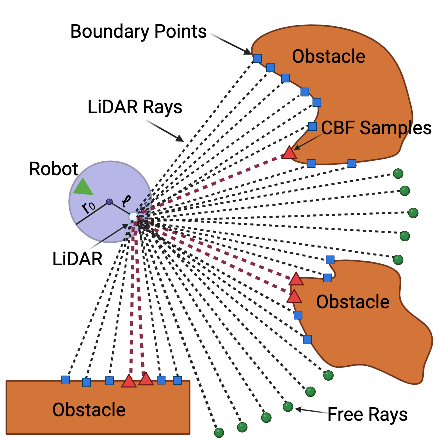
(b) Safe navigation

Figure 4: (a) A robot is depicted following a path generated by a motion planning algorithm, and a dynamic local reference goal is highlighted in yellow. (b) The robot sensing the environment with a $360$-degree LiDAR sensor mounted at $\tilde{\mathbf{x}}$. The CBF samples $\{h_{i}(\mathbf{x})\}_{i=1}^{N}$ are the rays with boundary points highlighted as red triangles, and are selected based on the distance from the LiDAR detections to the robot body.

In this section, we instantiate the control strategy developed in the previous sections to the case of unicycle dynamics in (7). We first design a CLF that enables stabilization to a desired goal point. Then, we discuss the validity of using a signed distance function (SDF) (Hoppe et al., 1992) as a CBF candidate for ensuring safety. Furthermore, we provide a discussion on how to select CBF samples based on range sensor measurements, which is crucial for the practical implementation of the distributionally robust safety constraint. By combining the unicycle-specific CLF and the data-driven CBF, we obtain a CLF-DR-CBF QP formulation tailored to the unicycle dynamics, enabling safe and efficient navigation in unknown dynamic environments.

8.1 Unicycle Stabilization to a Goal Position

We design a CLF that enables stabilization of the unicycle dynamics (7) to a desired goal point $\mathbf{q}_{G}\in\mathbb{R}^{2}$. We define the state space of the unicycle as ${\cal X}={\cal D}\times[-\pi,\pi)$, where ${\cal D}\subset\mathbb{R}^{2}$ is a sufficiently large compact set containing the environment of interest, including the goal point $\mathbf{q}_{G}$ and the planned path $\gamma$. This ensures that ${\cal X}$ is compact, satisfying Assumption 7.1.

Inspired by İşleyen et al. (2023), for a local reference point $\mathbf{q}\in\mathbb{R}^{2}$, we define $V$ as follows:

$$V(\mathbf{x})\!=\!\begin{cases}\frac{1}{2}(k_{v}\|\mathbf{q}\!-\!\phi(\mathbf{x})\|^{2}\!+\!k_{\omega}\text{atan2}(e_{v}^{\perp},e_{v})^{2}),&\!\phi(\mathbf{x})\!\neq\!\mathbf{q},\\ 0,&\!\phi(\mathbf{x})\!=\!\mathbf{q},\end{cases}$$ (29)

where $\phi(\mathbf{x})$ denotes the current robot position, and $k_{v},k_{\omega}>0$ are user-specified control gains for linear and angular errors. The error terms $e_{v}$ and $e_{v}^{\perp}$ are defined as:

$$e_{v}=\begin{bmatrix}\cos\theta\\ \sin\theta\end{bmatrix}^{\top}(\mathbf{q}-\phi(\mathbf{x})),\;e_{v}^{\perp}=\begin{bmatrix}-\sin\theta\\ \cos\theta\end{bmatrix}^{\top}(\mathbf{q}-\phi(\mathbf{x})).$$ (30)

When $\phi(\mathbf{x})\neq\mathbf{q}$, the first part of $V(\mathbf{x})$ represents the squared Euclidean distance between $\phi(\mathbf{x})$ and $\mathbf{q}$, while the second part quantifies the squared angular alignment error. Fig. 4(a) illustrates the unicycle robot tracking a local reference point $\mathbf{q}$ on the planned path.

The time derivative of $V(\mathbf{x})$ is:

$$\dot{V}(\mathbf{x})=\mathcal{L}_{\mathbf{g}}V(\mathbf{x})\mathbf{u}=\begin{bmatrix}-k_{v}e_{v}+k_{\omega}\dfrac{\text{atan2}(e_{v}^{\perp},e_{v})}{\|\mathbf{q}-\phi(\mathbf{x})\|^{2}}e_{v}^{\perp}\\ -k_{\omega}\text{atan2}(e_{v}^{\perp},e_{v})\end{bmatrix}^{\top}\mathbf{u}.$$ (31)

The following result provides a control law that ensures the satisfaction of the CLC in (2).

Lemma 8.1.

(Control Lyapunov constraint satisfaction): Let $\alpha_{V}$ be a class ${\cal K}$ function satisfying $\lim_{r\rightarrow 0^{+}}\frac{\alpha_{V}(r)}{r}=0$. For any state $\mathbf{x}\in{\cal X}$, the following control law

$$\mathbf{u}(\mathbf{x})=\begin{cases}-\alpha_{V}(V(\mathbf{x}))\frac{\mathcal{L}_{\mathbf{g}}V(\mathbf{x})^{\top}}{\|\mathcal{L}_{\mathbf{g}}V(\mathbf{x})^{\top}\|^{2}},\quad&\phi(\mathbf{x})\neq\mathbf{q},\\ \boldsymbol{0},\quad&\phi(\mathbf{x})=\mathbf{q},\end{cases}$$ (32)

ensures that $\mathcal{L}_{\mathbf{f}}V(\mathbf{x})+\mathcal{L}_{\mathbf{g}}V(\mathbf{x})\mathbf{u}(\mathbf{x})+\alpha_{V}(V(\mathbf{x}))\leq 0$ is satisfied. Furthermore, the control law is Lipschitz continuous for $\phi(\mathbf{x})\neq\mathbf{q}$ and continuous at $\mathbf{q}$.

Proof.

First, note that for any $\mathbf{x}\in{\cal X}$ such that $\phi(\mathbf{x})=\mathbf{q}$, we have $V(\mathbf{x})=0$ and $\mathcal{L}_{\mathbf{g}}V(\mathbf{x})=\boldsymbol{0}$, regardless of the orientation $\theta$. In this case, the control law $\mathbf{u}(\mathbf{x})$ given by (32) is simply $\boldsymbol{0}$, which trivially satisfies the CLC: $\mathcal{L}_{\mathbf{f}}V(\mathbf{x})+\mathcal{L}_{\mathbf{g}}V(\mathbf{x})\mathbf{u}(\mathbf{x})+\alpha_{V}(V(\mathbf{x}))\leq 0$.

Next, we show that $\mathcal{L}_{\mathbf{g}}V(\mathbf{x})\neq\boldsymbol{0}$ for all $\mathbf{x}\in{\cal X}$ such that $\phi(\mathbf{x})\neq\mathbf{q}$. Suppose, by contradiction, that $\mathcal{L}_{\mathbf{g}}V(\mathbf{x})=\boldsymbol{0}$. This implies $k_{\omega}\text{atan2}(e_{v}^{\perp},e_{v})=0$, which means $e_{v}^{\perp}=0$. From (30), we have $e_{v}^{2}+e_{v}^{\perp^{2}}=(\mathbf{q}-\phi(\mathbf{x}))^{2}$. Since $e_{v}^{\perp}=0$ and $\phi(\mathbf{x})\neq\mathbf{q}$, we obtain $e_{v}=\pm|\mathbf{q}-\phi(\mathbf{x})|\neq 0$, contradicting the assumption that $\mathcal{L}_{\mathbf{g}}V(\mathbf{x})=\boldsymbol{0}$. Hence, $\mathcal{L}_{\mathbf{g}}V(\mathbf{x})\neq\boldsymbol{0}$ for all $\mathbf{x}\in{\cal X}$ such that $\phi(\mathbf{x})\neq\mathbf{q}$.

Now, for all $\mathbf{x}\in{\cal X}$ such that $\phi(\mathbf{x})\neq\mathbf{q}$, the control law $\mathbf{u}(\mathbf{x})$ given by (32) is the closed-form solution to the optimization problem:

$$\min_{\mathbf{u}\in\mathbb{R}^{m}}\|\mathbf{u}\|^{2},$$ (33)

$$\mathrm{s.t.}\,\, \mathcal{L}_{\mathbf{g}}V(\mathbf{x})\mathbf{u}+\alpha_{V}(V(\mathbf{x}))\leq 0.$$

Since $V(\mathbf{x})$ is smooth with bounded derivatives for $\phi(\mathbf{x})\neq\mathbf{q}$, it follows that $\mathbf{u}(\mathbf{x})$ is Lipschitz continuous on the set $\{\mathbf{x}\in{\cal X}:\phi(\mathbf{x})\neq\mathbf{q}\}$.

Next, to show continuity on ${\cal X}$, we prove that $\lim_{\mathbf{x}\rightarrow\mathbf{x}_{G}}\mathbf{u}(\mathbf{x})=\boldsymbol{0}$ for any $\mathbf{x}_{G}\in{\cal X}$ such that $\phi(\mathbf{x}_{G})=\mathbf{q}$. Based on (31), we can write

$$\lim_{\mathbf{x}\rightarrow\mathbf{x}_{G}}|\mathbf{u}(\mathbf{x})|=\lim_{\mathbf{x}\rightarrow\mathbf{x}_{G}}\left|\alpha_{V}(V(\mathbf{x}))\frac{\mathcal{L}{\mathbf{g}}V(\mathbf{x})^{\top}}{\|\mathcal{L}{\mathbf{g}}V(\mathbf{x})^{\top}\|^{2}}\right|$$

$$\leq\lim_{\mathbf{x}\rightarrow\mathbf{x}_{G}}\frac{\alpha_{V}(V(\mathbf{x}))}{V(\mathbf{x})}\cdot\lim_{\mathbf{x}\rightarrow\mathbf{x}_{G}}\left|\frac{V(\mathbf{x})}{\|\mathcal{L}{\mathbf{g}}V(\mathbf{x})^{\top}\|}\right|=0,$$

where the last equality holds because the first limit is zero by the assumption on $\alpha_{V}$, and the second limit is bounded since $\frac{V(\mathbf{x})}{|\mathcal{L}{\mathbf{g}}V(\mathbf{x})^{\top}|}$ remains bounded as $\mathbf{x}\rightarrow\mathbf{x}_{G}$. Therefore, the control law $\mathbf{u}(\mathbf{x})$ is continuous on ${\cal X}$. ∎∎

The control law minimizes the norm of $\mathbf{u}$ while ensuring $\dot{V}(\mathbf{x})<0$. Therefore, the function $V$ in (29) together with the control law $\mathbf{u}(\mathbf{x})$ in (32) satisfy Assumption 7.2. Therefore, Lemma 7.3 ensures that the system is guided towards the goal point $\mathbf{q}$. Since the control law $\mathbf{u}(\mathbf{x})=\boldsymbol{0}$ whenever $\phi(\mathbf{x})=\mathbf{q}$, the orientation $\theta(t)$ may converge to any value, depending on the initial conditions. Finally, by Theorem 7.5, the closed-loop dynamics interconnected with the governor dynamics has the unicycle robot track the planned path $\gamma$ in $\mathbb{R}^{2}$.

8.2 Signed Distance Function as Control Barrier Function

In unknown and dynamic environments, the precise computation of the barrier function $h(\mathbf{x},t)$ or the construction of a probabilistic model is challenging. Therefore, this section focuses on safe control synthesis, directly leveraging the distance measurements $\boldsymbol{\eta}(\phi(\mathbf{x})_{s},\mathbf{R}_{s})=[\eta_{1}(\phi(\mathbf{x})_{s},\mathbf{R}_{s}),...,\eta_{K}(\phi(\mathbf{x})_{s},\mathbf{R}_{s})]^{\top}$ to define the safety constraint.

Given that the range sensor is mounted at $\phi(\mathbf{x})_{s}=[x+l\cos(\theta),y+l\sin(\theta)]^{\top}\in\mathbb{R}^{2}$, we describe the dynamics of $\mathbf{x}_{s}=[x+l\cos(\theta),y+l\sin(\theta),\theta]^{\top}$ as outlined by Cortés and Egerstedt (2017):

$$\dot{\mathbf{x}}_{s}=\underbrace{\left[\begin{matrix}\cos(\theta)&-l\sin(\theta)\\ \sin(\theta)&l\cos(\theta)\\ 0&1\end{matrix}\right]}_{\tilde{\mathbf{g}}(\mathbf{x})}\left[\begin{matrix}v\\ \omega\end{matrix}\right].$$ (34)

Next, we discuss the validity of using the signed distance function from the robot position to the obstacle set ${\cal O}(t)$ as a time-varying CBF candidate for the dynamics (34). The signed distance function $\varphi:\mathbb{R}^{2}\times\mathbb{R}\mapsto\mathbb{R}$ of set ${\cal O}(t)$ is:

$$\varphi(\phi(\mathbf{x}),t):=\begin{cases}-d(\phi(\mathbf{x}),\partial{\cal O}(t)),&\phi(\mathbf{x})\in{\cal O}(t),\\ \phantom{-}d(\phi(\mathbf{x}),\partial{\cal O}(t)),&\phi(\mathbf{x})\notin{\cal O}(t).\end{cases}$$ (35)

The distance function provides a useful measure of safety, with positive values indicating free space. We exploit this property to construct a CBF that ensures the safety of the system dynamics described in (34).

Let $r_{0}$ denote the robot radius, as shown in Fig. 4(b). To ensure the safety of the entire robot body ${\cal B}(\mathbf{x})$, we define the candidate CBF as

$$h(\mathbf{x},t)=\varphi(\phi(\mathbf{x})_{s},t)-r_{0}-l,$$ (36)

which ensures that the safety margin accounts for both the robot body and the placement of the LiDAR. The next result shows that $h(\mathbf{x},t)$ in (36) is a valid time-varying CBF candidate for the dynamics in (34).

Lemma 8.2.

(Signed distance function as a time-varying control barrier function): Assume that the partial time derivative of the signed distance function is bounded, i.e., there exists a constant $B>0$ such that $\left|\frac{\partial\varphi(\phi(\mathbf{x})_{s},t)}{\partial t}\right|\leq B$ for all $\phi(\mathbf{x})_{s}\in{\cal D}\subset\mathbb{R}^{2}$ and $t\in\mathbb{R}$. Then, the function $h(\mathbf{x},t)$ in (36) is a valid time-varying CBF for the system dynamics (34).

Proof.

From the dynamics model (34), the derivative of the candidate time-varying CBF along the system dynamics is:

$$\dot{h} (\mathbf{x},t)=\nabla\varphi(\phi(\mathbf{x})_{s},t)^{\top}\dot{\phi(\mathbf{x})}_{s}+\frac{\partial\varphi(\phi(\mathbf{x})_{s},t)}{\partial t}$$

$$=\nabla\varphi(\phi(\mathbf{x})_{s},t)^{\top}\begin{bmatrix}v\cos(\theta)\!-\!l\omega\sin(\theta)\\ v\sin(\theta)\!+\!l\omega\cos(\theta)\end{bmatrix}\!+\!\frac{\partial\varphi(\phi(\mathbf{x})_{s},t)}{\partial t}$$

$$=\nabla\varphi(\phi(\mathbf{x})_{s},t)^{\top}R(\theta)\mathbf{u}_{l}+\frac{\partial\varphi(\phi(\mathbf{x})_{s},t)}{\partial t},$$

where $\mathbf{u}_{l}=[v,l\omega]^{\top}$, $R(\theta)=\begin{bmatrix}\cos(\theta)&-\sin(\theta)\\ \sin(\theta)&\cos(\theta)\end{bmatrix}$. It is known (Crandall and Lions, 1983) that the gradient $\nabla\varphi(\phi(\mathbf{x})_{s},t)$ of the signed distance function is well-defined and has a unit norm near the boundary of the obstacle set ${\cal O}(t)$ . Next, by choosing $\mathbf{u}_{l}=R(-\theta)\mathbf{p}$, where $\mathbf{p}=\beta\nabla\varphi(\phi(\mathbf{x})_{s},t)$, $\beta>0$ is a scaling factor, we have

$$\dot{h}(\mathbf{x})=\beta\|\nabla\varphi(\phi(\mathbf{x})_{s},t)\|^{2}+\frac{\partial\varphi(\phi(\mathbf{x})_{s},t)}{\partial t}\geq\beta-B.$$ (37)

The scaling factor $\beta$ can be chosen sufficiently large such that $\beta>B$, ensuring $\dot{h}(\mathbf{x},t)>0$ near the boundary of the obstacle set. Therefore, $h(\mathbf{x},t)$ in (36) is a valid time-varying CBF for (34). ∎∎

From a practical perspective, it is important to note that, if there are bounds on the control inputs, e.g., $|v|\leq v_{\max}$ and $|\omega|\leq\omega_{\max}$, then the scaling factor $\beta$ in the proof of Lemma 8.2 must be chosen to ensure that $\mathbf{u}_{l}$ satisfies these constraints while maintaining $\dot{h}(\mathbf{x},t)>0$ near the boundary of the obstacle set. This means that the bound $B$ on the partial time derivative of the distance function must be compatible with the control bounds to ensure the inequality (37) holds. In other words, the obstacles must move at speeds compatible with the motion capabilities of the unicycle to guarantee safety.

8.3 Sensor-Based CBF Sample Selection

As the robot navigates, we continuously collect range sensor measurements and their corresponding time derivatives, which represent the rate of change of detected distances, denoted as $\frac{\partial\boldsymbol{\eta}}{\partial t}(\phi(\mathbf{x})_{s},\mathbf{R}_{s},t)\in\mathbb{R}^{K}$. This can be estimated by a radar sensor, Doppler LiDAR, or LiDAR velocity algorithms (Yang et al., 2022). In the following, we discuss our approach to obtain samples $\{\boldsymbol{\xi}\}_{i\in[N]}$ by leveraging such measurements.

We collect LiDAR measurements from the last few frames. To account for the robot’s movement, these measurements are transformed to align with the robot’s current pose. From this aggregated data, we select $N$ samples with the lowest values of $\frac{\partial h(\mathbf{x},t)}{\partial t}+\alpha_{h}(h(\mathbf{x},t))$. This criterion is chosen because it effectively identifies those obstacle boundary points where the combined effect of the rate of change in the environment and the current state of the barrier function is most critical. This highlights those samples where the safety constraint, defined in (5), is closest to being violated.

For each selected sample $\{h_{i}(\mathbf{x},t),\frac{\partial h_{i}}{\partial t}\}$, the corresponding gradient $\nabla_{\mathbf{x}}h_{i}(\mathbf{x},t)$ is computed as follows. Let $\mathbf{q}_{i}$ represent the position in the environment corresponding to the LiDAR-detected point for the $i$-th measurement. The vector from the robot’s position $\phi(\mathbf{x})$ to $\phi(\mathbf{x})_{i}$ is given by $\mathbf{v}_{i}=\phi(\mathbf{x})_{i}-\phi(\mathbf{x})$. The gradient of the sample is determined as:

$$\nabla_{\mathbf{x}}h_{i}(\mathbf{x},t):=\left[\frac{\mathbf{v}_{i}}{\|\mathbf{v}_{i}\|},0\right]^{\top}.$$ (38)

The normalization is essential because the SDF, by its Eikonal property (Crandall and Lions, 1983), has a gradient with a unit 2-norm. The appended zero reflects the fact that the constructed CBF is independent of the robot’s orientation $\theta$. With this procedure, given each $\mathbf{x}\in{\cal X}$, we have available samples $\{\boldsymbol{\xi}_{i}\}_{i\in[N]}$ for the vector $\boldsymbol{\xi}$.

Remark 8.3.

(Sample selection for static environments): If $\frac{\partial h}{\partial t}=0$, the selection of the $N$ samples reduces to finding the minimum $N$ values of $h_{i}(\mathbf{x})$, representing the distance of $N$ closest detected obstacle points to the robot. This is illustrated in Fig. 4(b).  $\bullet$

With the sample collection strategy for $\{\boldsymbol{\xi}_{i}\}_{i\in[N]}$ and the CLF design in (29), we formulate the CLF-DR-CBF optimization problem in (18) to synthesize control inputs for the unicycle robot. The unicycle-specific CLF is combined with the DR-CBF constraint, which is based on the CBF samples obtained from the range sensor measurements. This approach enables safe robot navigation in unknown dynamic environments, while directly utilizing the sensor measurements to ensure safety.

9 Evaluation

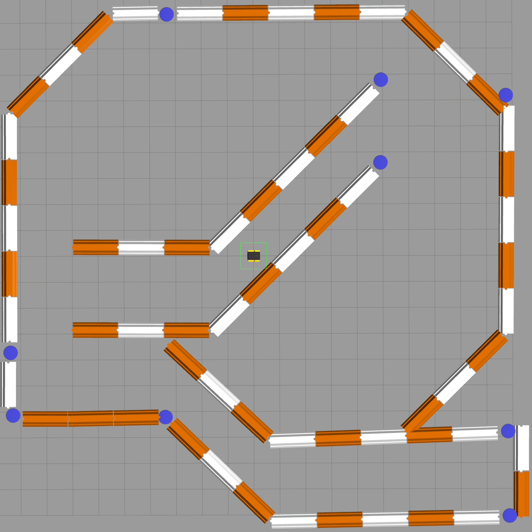
(a) Static environment

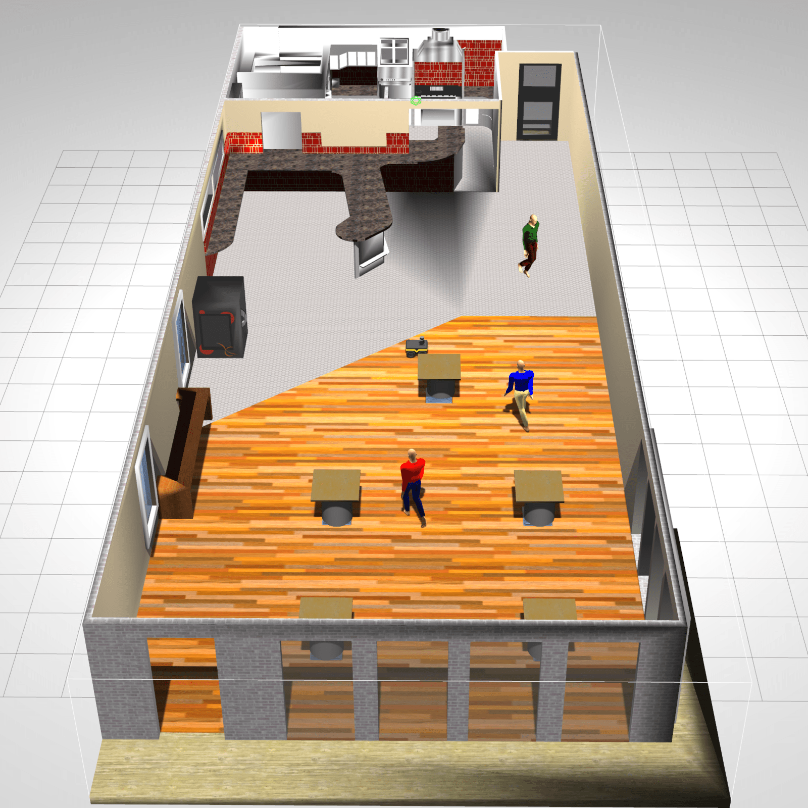
(b) Dynamic environment

Figure 5: Simulated environments in Gazebo.

In this section, we evaluate our CLF-DR-CBF QP formulation through several simulation and real-world experiments.

We compare our approach with two other safe control strategies, the nominal CLF-CBF QP in (6) and a CLF-Gaussian Process (GP)-CBF second-order cone program (SOCP) (Long et al., 2022). The nominal CLF-CBF QP approach utilizes the closest LiDAR point to define a single CBF $h(\mathbf{x},t)$ and its gradients at each time step. In the CLF-GP-CBF SOCP method, a real-time GP-SDF model (Wu et al., 2021) of the unknown environment is constructed using LiDAR data, from which the CBF, its gradient, and uncertainty information are determined. For a fair evaluation, we solve each of the optimization programs to generate control signals using the Splitting Conic Solver in CVXPY (Agrawal et al., 2018).

In the following simulations and experiments, a consistent set of parameters is utilized to ensure comparability and reproducibility of the results. The linear velocity is constrained between $[-1.2,1.2]$ m/s and the angular velocity is limited within $[-1,1]$ rad/s. The nominal control input $\mathbf{k}(\mathbf{x})$ is set to $[1.2,0]^{\top}$ (the unicycle is commanded to move forward at a speed of 1.2 m/s) and the scaling factor is $\lambda=50$. Table 1 summarizes other parameter values.

Table 1: Simulation and experiment parameters. The class ${\cal K}$ function $\alpha_{V}$ for CLF is assumed to be linear, and $a$ is the linear CBF class ${\cal K}_{\infty}$ function. The parameters $k_{v}$ and $k_{\omega}$ are control gains for linear and angular velocities, respectively, $l$ is the LiDAR offset distance, $\epsilon$ the risk tolerance of the CLF-DR-CBF QP formulation, and $N$ the DR-CBF sample size.

Param.	$\alpha_{V}$	$a$	$k_{v}$	$k_{\omega}$	$l$ (m)	$\epsilon$	$N$
Value	1.0	0.4	0.05	0.4	0.08	0.1	5

Sec. 9.1 presents simulation results and compares with the two baseline approaches in a static environment in the Gazebo physics simulator (Koenig and Howard, 2004), shown in Fig. 5(a). In Sec. 9.2, we evaluate our approach in dynamic Gazebo environments with pedestrians, shown in Fig. 5(b). Finally, in Sec. 9.3, we test our CLF-DR-CBF QP formulation in cluttered dynamic real-world environments. In all results, the $A^{*}$ algorithm is employed for path planning, operating at a frequency of $5$ Hz. Our CLF-DR-CBF QP formulation is used for real-time obstacle avoidance, running at $50$ Hz.

9.1 Simulated Static Environments

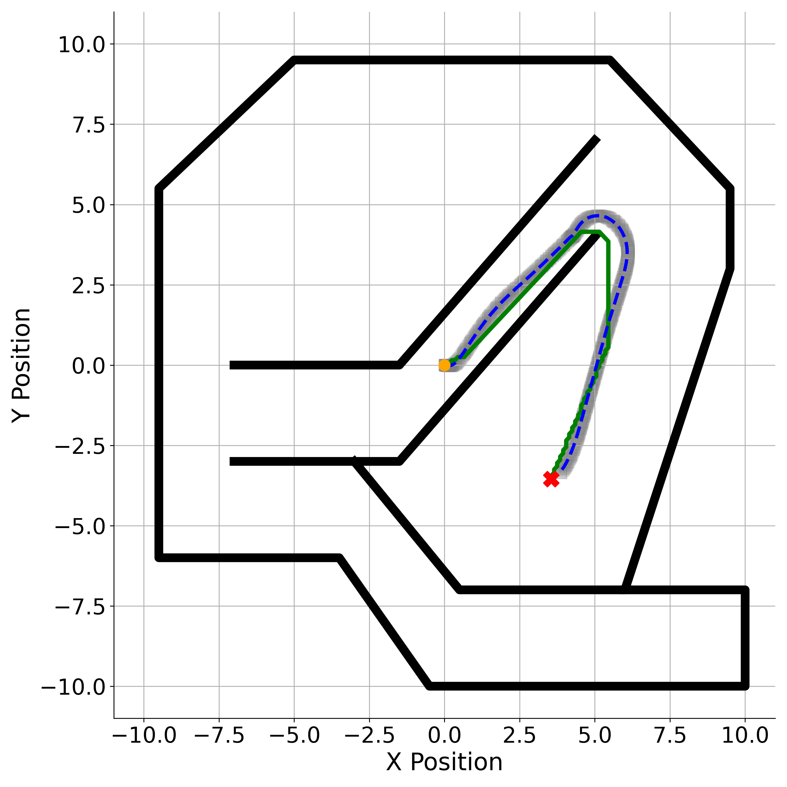
(a)

(b)

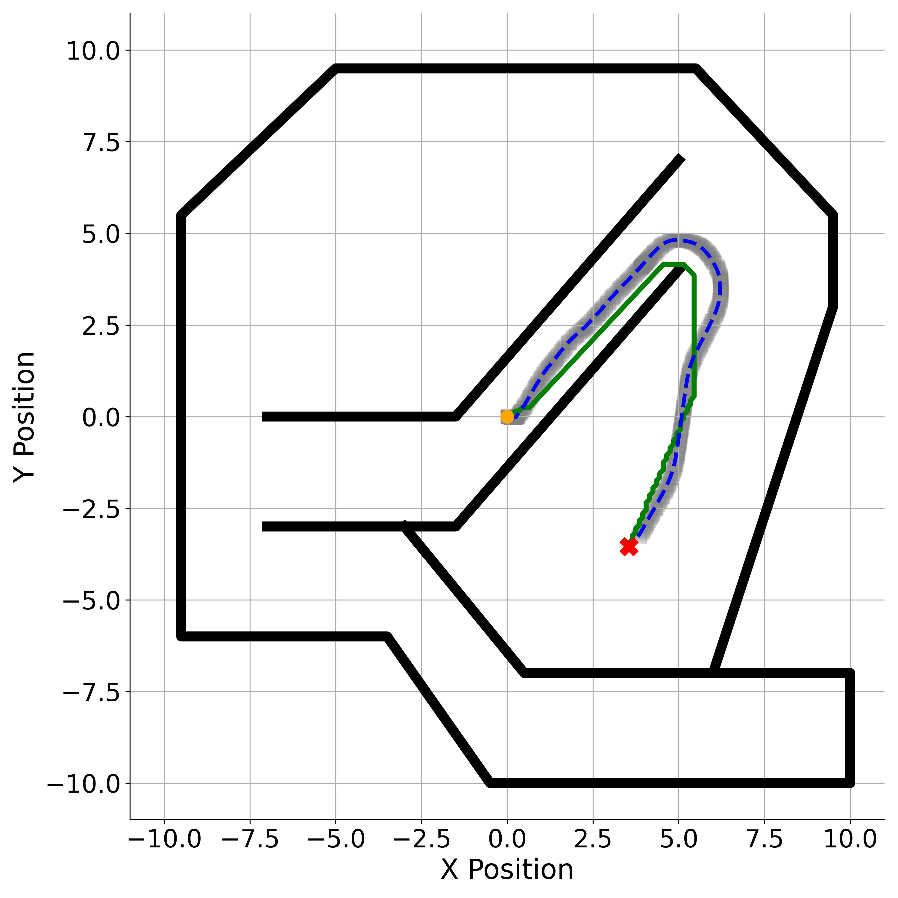
(c)

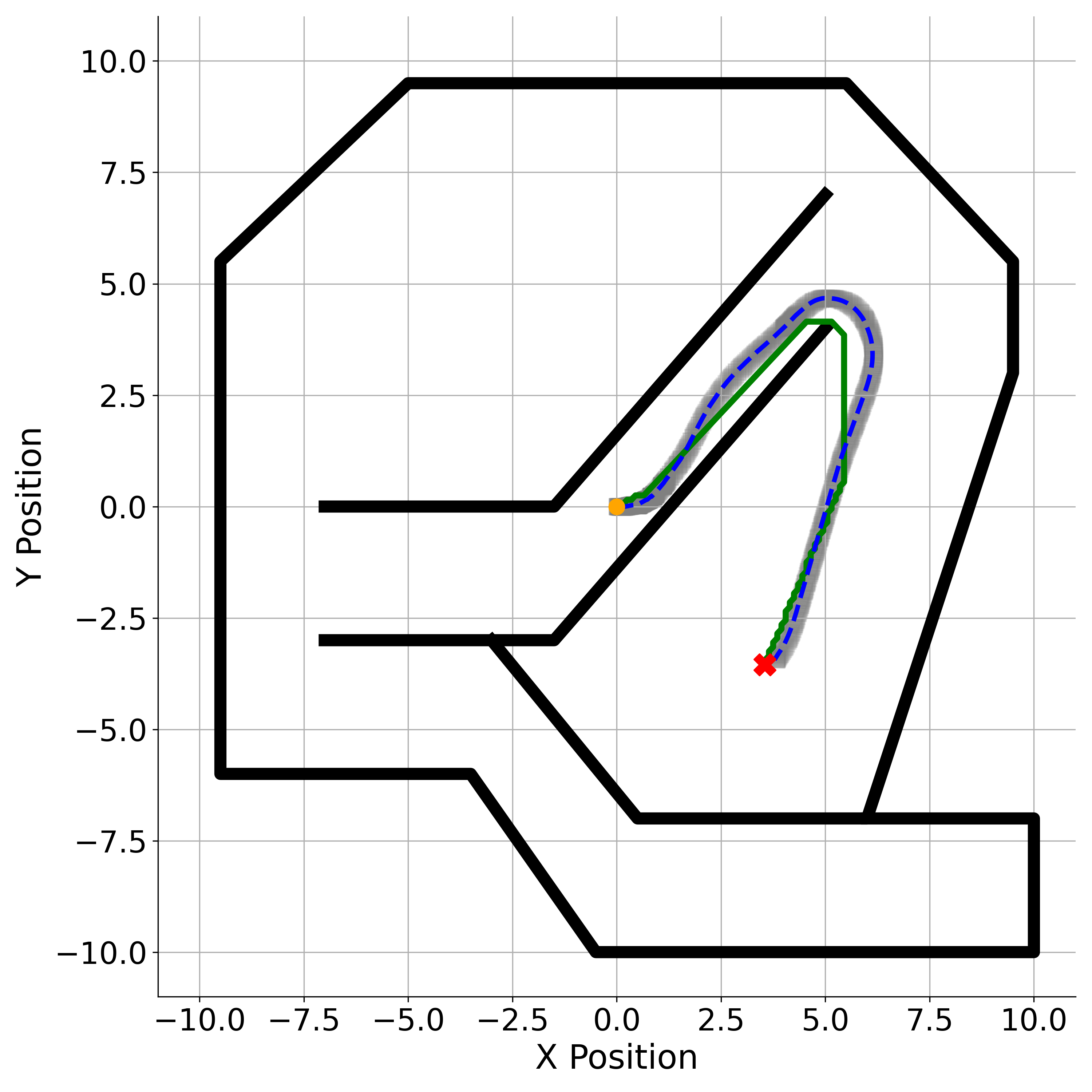
(d)

Figure 6: Comparison of robot trajectories under DR-CBF, GP-CBF, and baseline CBF QP formulations with varying LiDAR noise levels. The planned $A^{*}$ path is shown in green, the actual robot paths in dashed blue, and the robot’s footprint over time as shaded areas. The start and goal points are marked yellow and red, respectively, with an initial orientation of $\theta=0$.

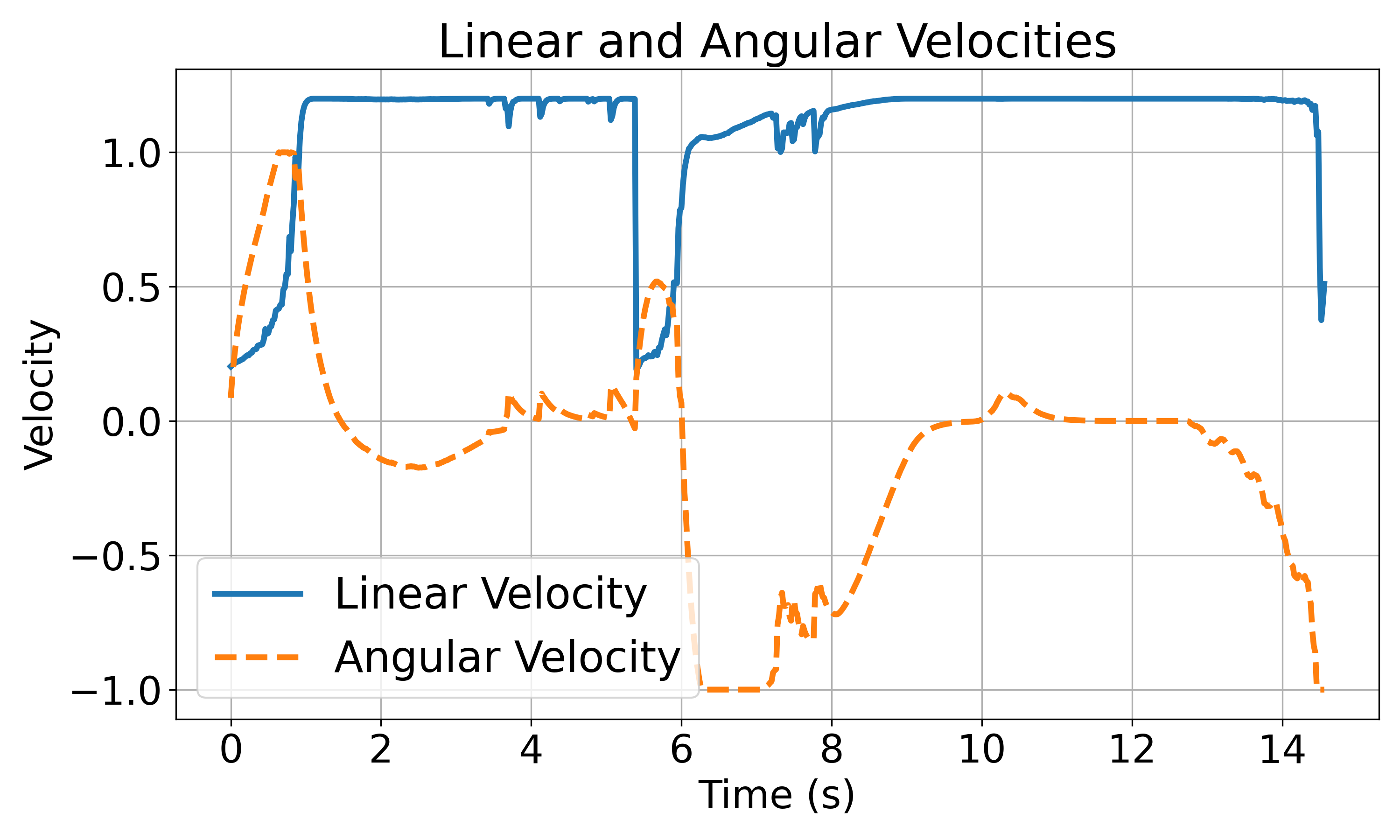
(a)

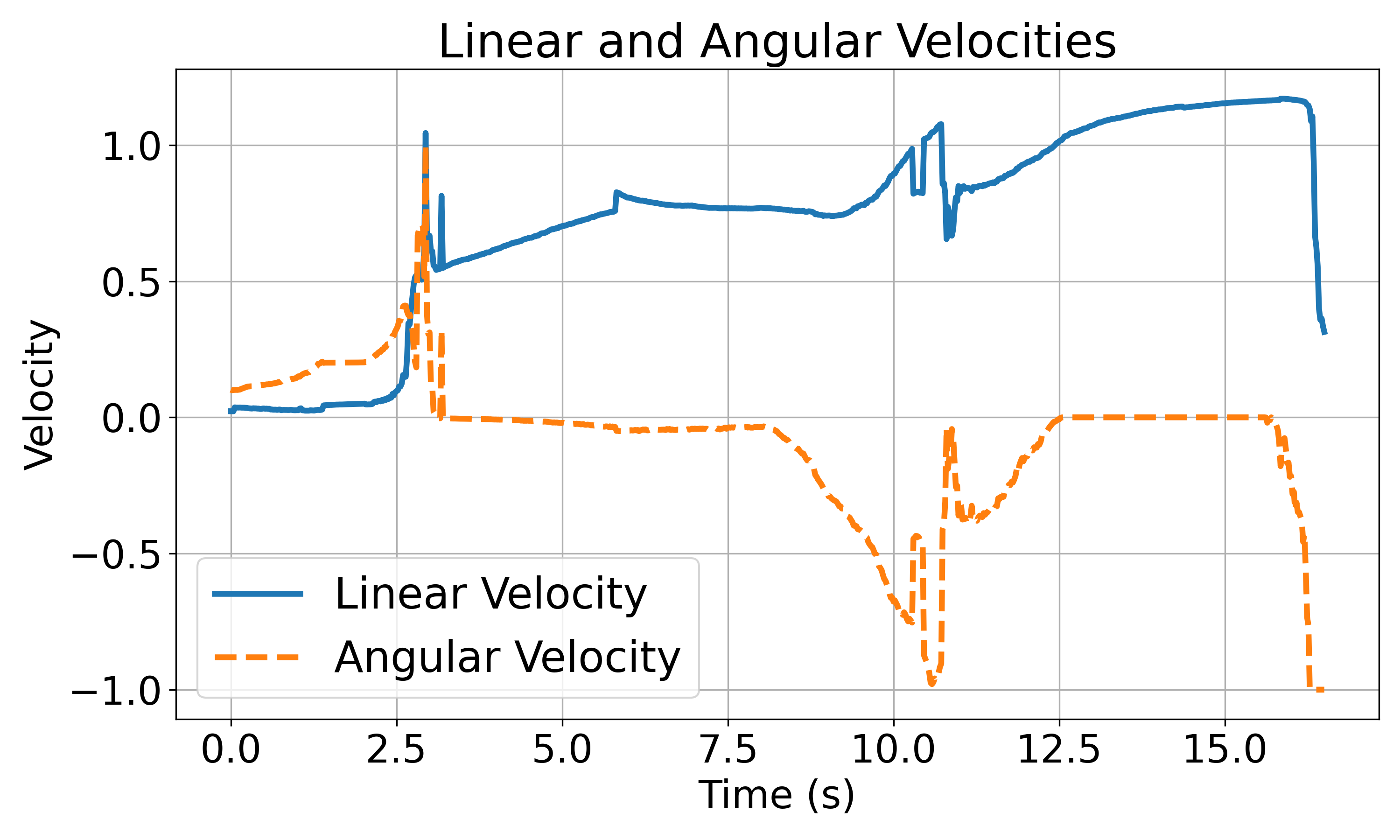
(b)

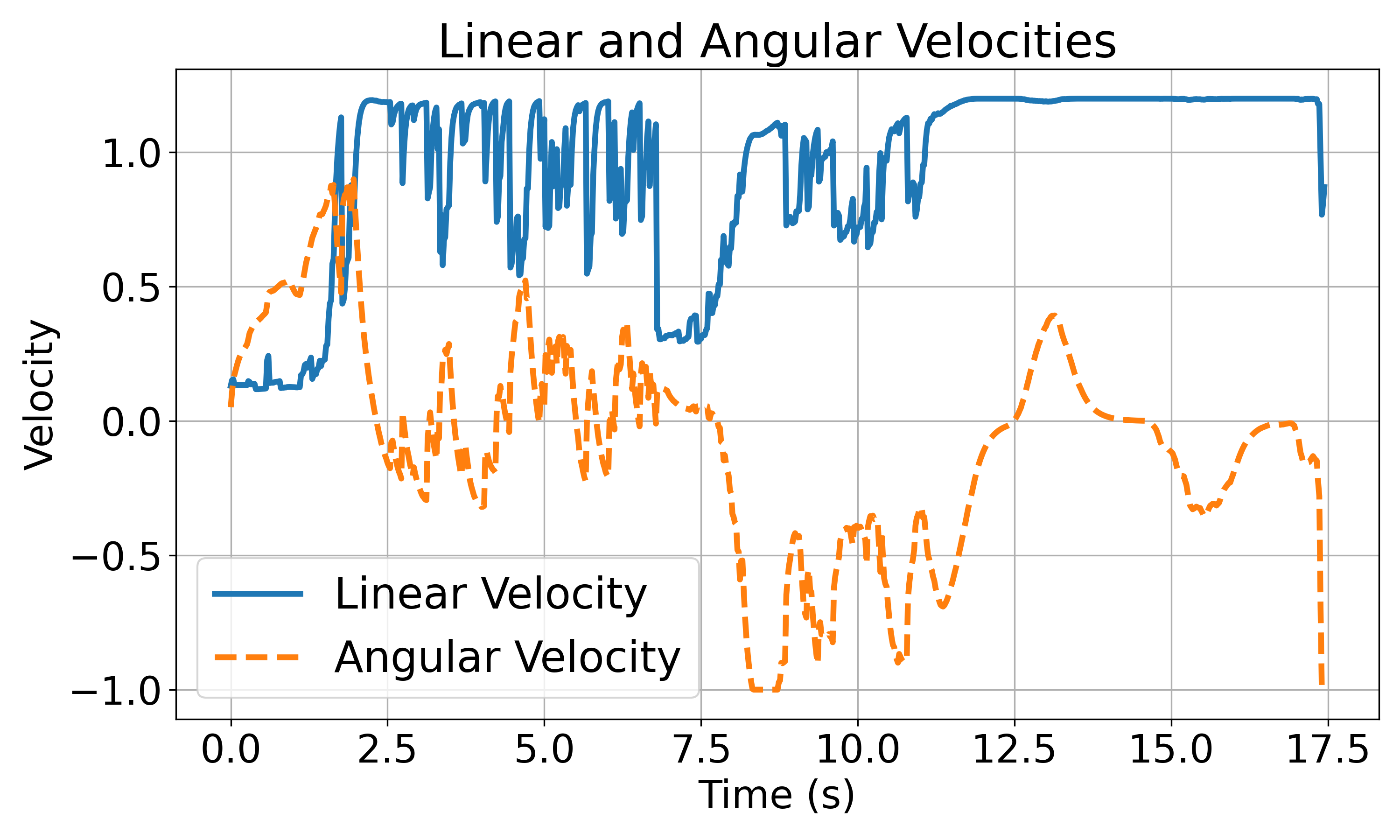
(c)

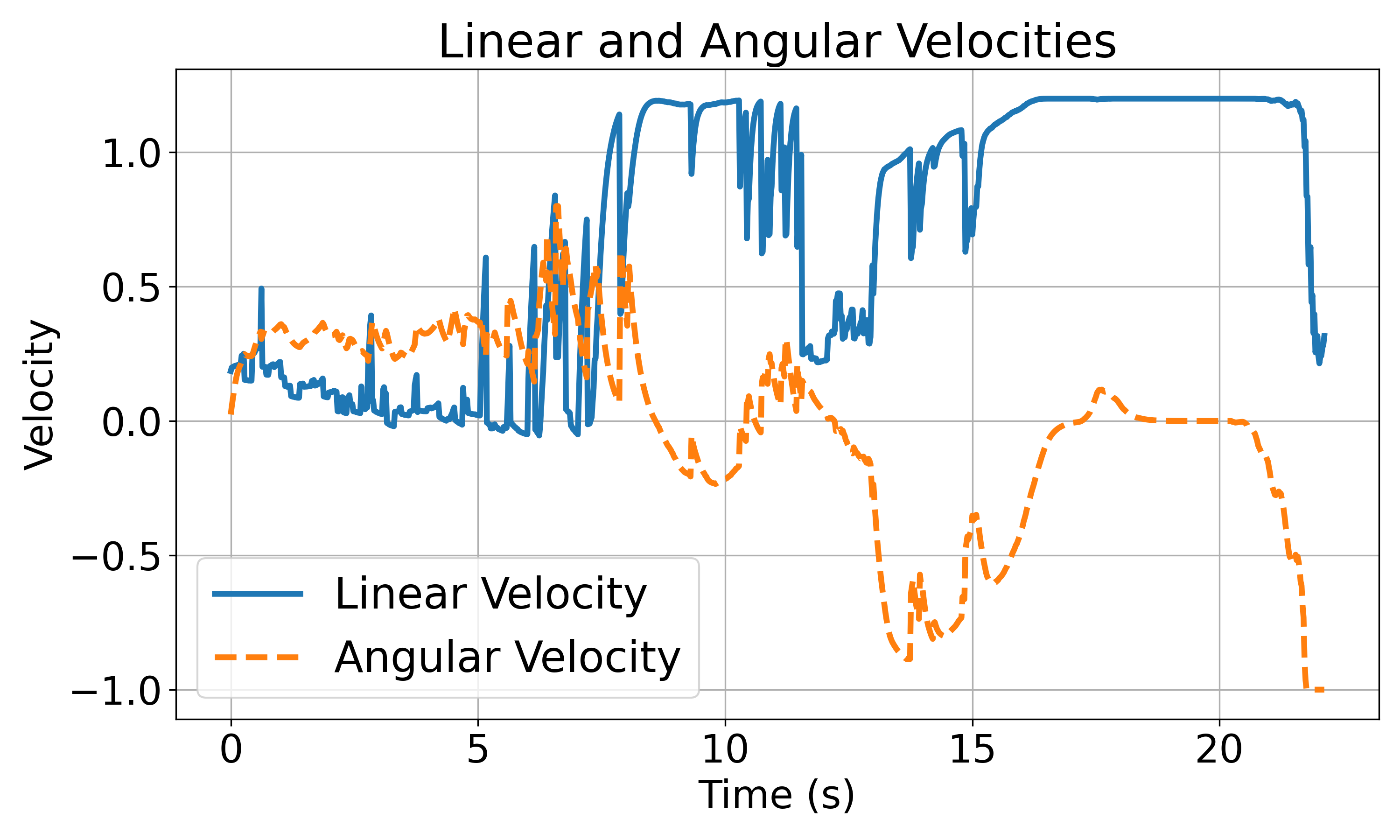
(d)

Figure 7: Velocity profile comparisons of different control methods under varying LiDAR noise.

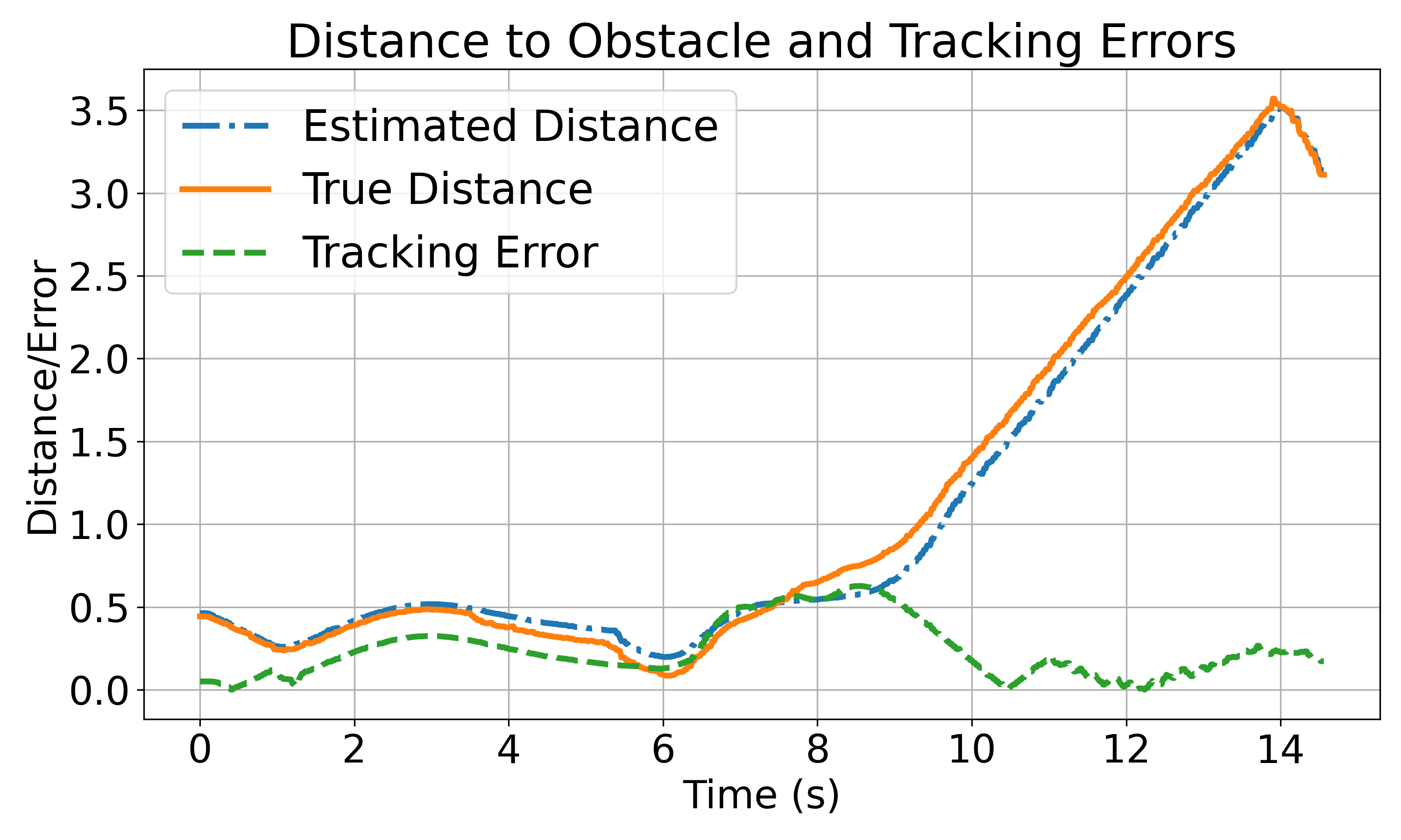
(a)

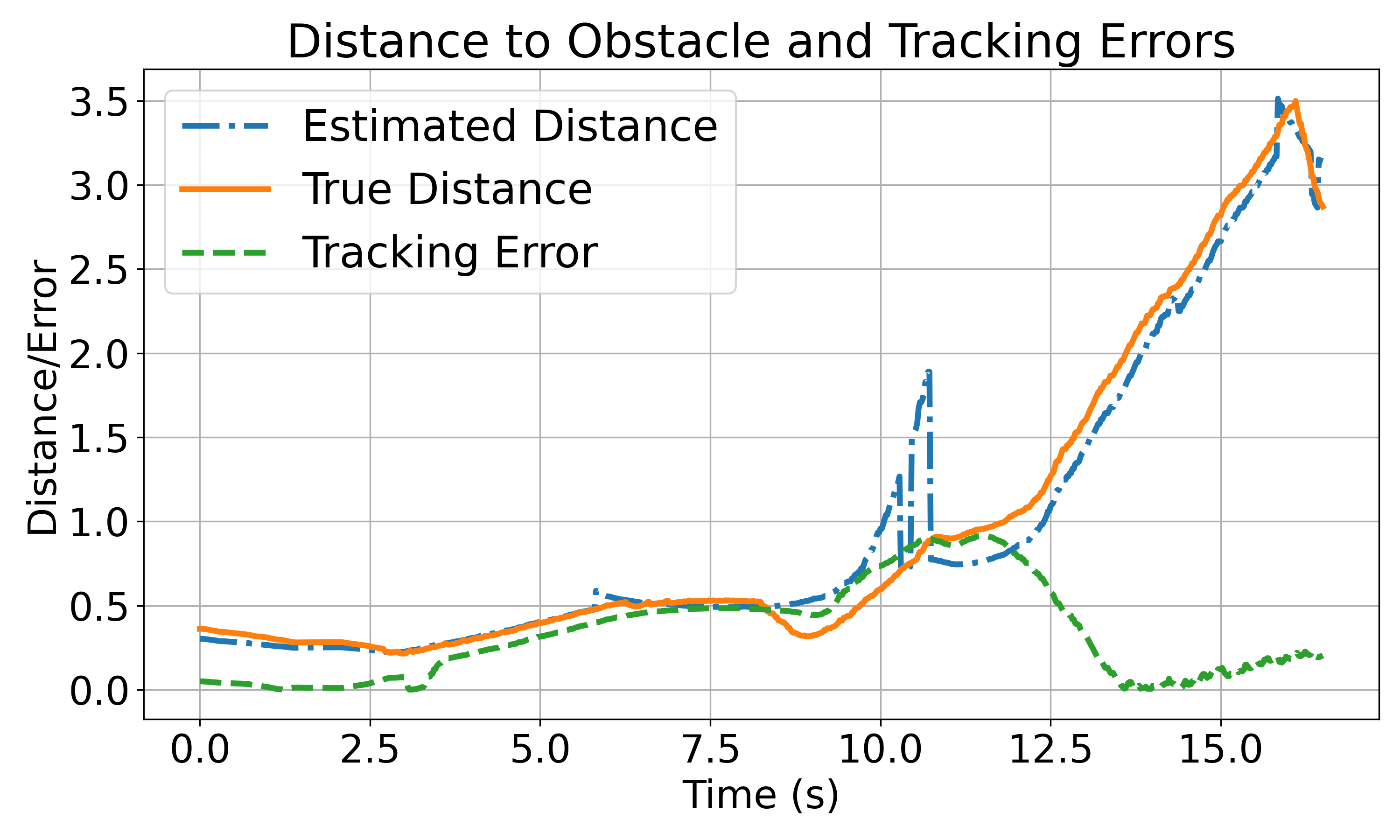
(b)

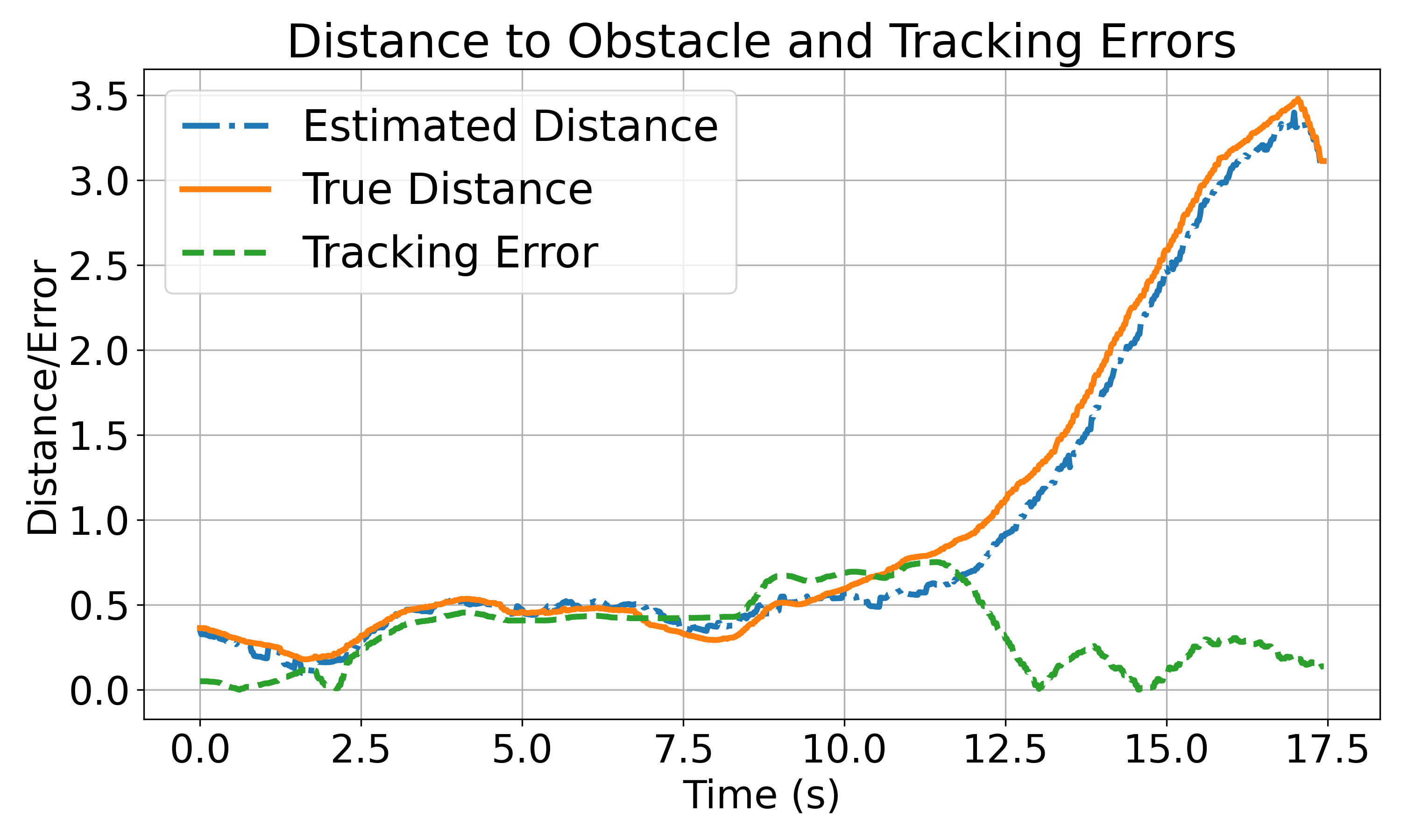
(c)

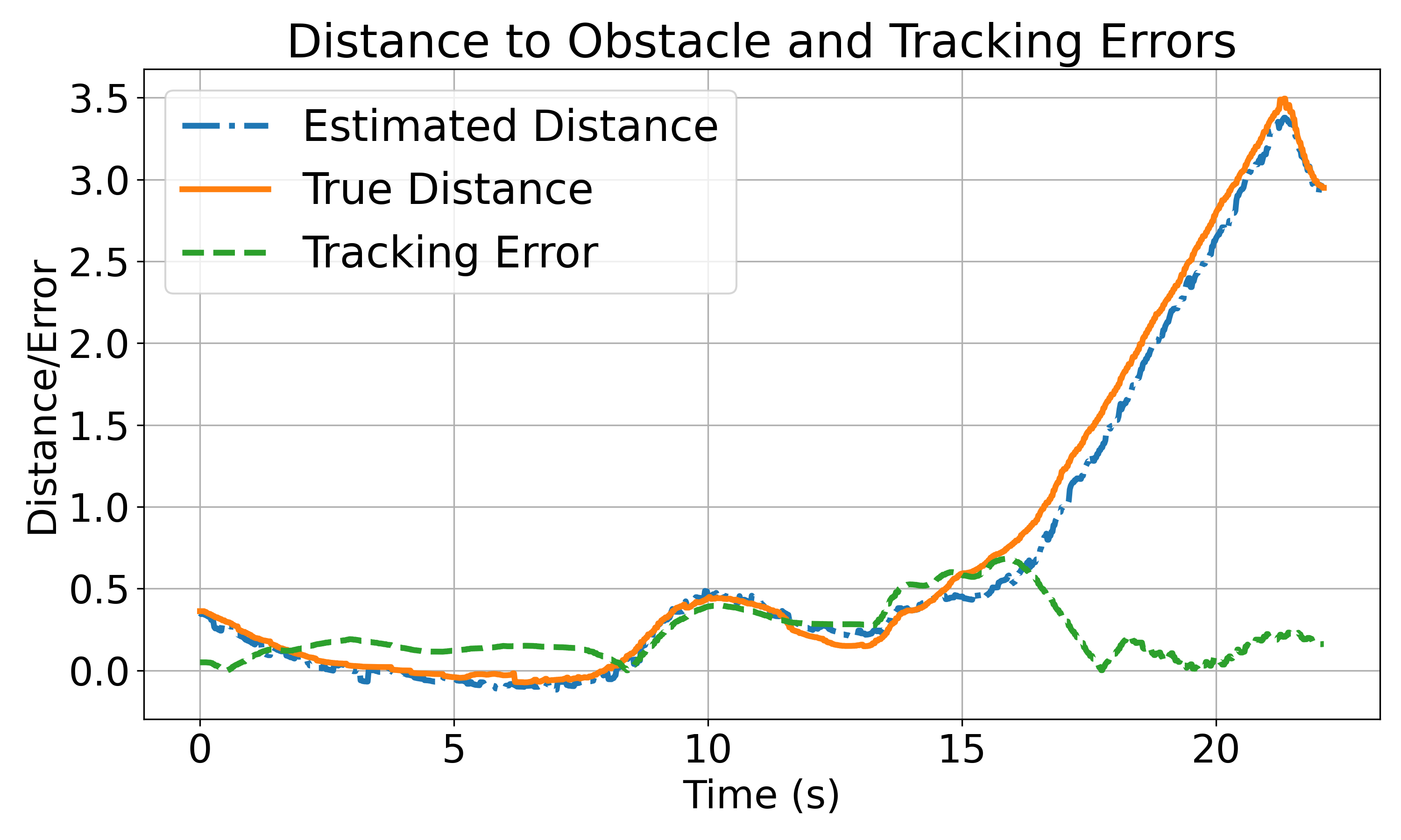
(d)

Figure 8: Evaluation of the estimated distance, true distance, and tracking errors under different control strategies. For the estimated distance to obstacles, the DR and the nominal methods use the closest LiDAR distance measurements, while the GP-CBF method uses the reconstructed GP-SDF model. The tracking error is computed as the distance between the robot’s position and its closest point on the planned path.

The first set of simulations demonstrates our approach in static environments with varying LiDAR noise, as shown in Fig. 5(a). The robot is tasked to track a planned path (shown in green in Fig. 6) safely in an unknown environment, relying on noisy LiDAR measurements. We introduce Gaussian noise with standard deviation $\sigma$ (ranging from $0.001$ to $0.05$) to each distance measurement of every LiDAR scan. The planned path is not safe for the robot in general, since it does not take the sensing noise into account. Figs. 6–8 compare our method with the two baselines under different noise levels on the LiDAR measurements. All simulations were conducted on a computer with an Intel i9-12900K CPU with 64 GB RAM.

Table 2: Computation time comparison between different control approaches (in seconds). The values represent the mean $\pm$ standard deviation of the computation time along the trajectory shown in Fig. 6. The total computation time for each method is the sum of the GP map training time (if applicable), inference time, and control synthesis solver time. The CLF-DR-CBF QP and Nominal CLF-CBF QP methods have similar total computation time, as they do not require GP map training. For these two methods, the inference time refers to processing the LiDAR data as CBF samples and corresponding gradients. The CLF-GP-CBF SOCP method has the highest total computation time due to the additional overhead of GP map training.

Method	Map Training	Inference	Controller Solver	Total Computation Time
CLF-DR-CBF QP	0	0.0001	0.0098 ± 0.0027	0.0099 ± 0.0027
CLF-GP-CBF SOCP	0.0086 ± 0.0031	0.0003	0.0119 ± 0.0034	0.0208 ± 0.0065
Nominal CLF-CBF QP	0	0.0001	0.0092 ± 0.0033	0.0093 ± 0.0033

In Figs. 6(a), 7(a), and 8(a), we employ our CLF-DR-CBF QP approach to synthesize controls for the robot with Wasserstein radius set to be $r=0.004$. The robot reaches the goal safely in about 14 seconds, demonstrating efficiency and safety in a low-noise regime. Comparing this to the CLF-GP-CBF SOCP strategy (Figs. 6(b), 7(b), and 8(b)) under the same noise conditions suggests comparable results in path following and safety. However, as shown in Table 2, our CLF-DR-CBF approach benefits from direct LiDAR data processing, bypassing the GP model’s computational overhead for map training and updates. Besides, as illustrated in Fig. 7(b), during the initial 2-second interval, the robot’s movement under the CLF-GP-CBF SOCP controller is noticeably slower. This reduced speed results from the GP-SDF’s need to accumulate a sufficient volume of LiDAR data for model training, where the initial high estimated CBF variance, due to limited data, constrains rapid movement. Furthermore, as shown in Fig. 8(b), it may be challenging for the GP-SDF to estimate the precise distance to obstacles at around $t=10$s, where the robot is at the top right corner.

When the LiDAR sensor noise level is elevated to $\sigma=0.05$, the variance in the GP-SDF estimation exhibits a substantial increase. This heightened variance can severely undermine the practical applicability of the CLF-GP-CBF SOCP controller, leading to infeasibility of the formulation. Therefore, we do not present the results for the CLF-GP-CBF SOCP controller in this scenario. On the other hand, our CLF-DR-CBF QP controller still works, as shown in Fig. 6(c) to Fig. 8(c). In particular, to account for the larger noise in the measurements, we increased the Wasserstein radius $r$ from $0.004$ to $0.006$. The results underscore the advantage of handling noisy sensor data directly in our formulation without reliance on accurate map estimation.

Comparing Fig. 7(c) to Fig. 7(a), with the CLF-DR-CBF QP controller, we observe that the time needed to complete the task is longer and the control inputs are less smooth due to the larger noise in the LiDAR measurements. However, as shown in Fig. 6(c) and Fig. 8(c), our approach still effectively tracks the planned path and maintains safety. Under the same noise level, we compare our approach with the nominal CLF-CBF QP approach. As shown in Figs. 7(d) and 8(d), the baseline approach requires a longer time to achieve the goal and fails to maintain a safe distance from the obstacle, with a minimum distance of $-0.07$m at around $t=7$s, as evident in Fig. 8(d). This negative distance indicates that the baseline approach violates the safety constraints and comes close to colliding with the obstacle.

9.2 Simulated Dynamic Environments

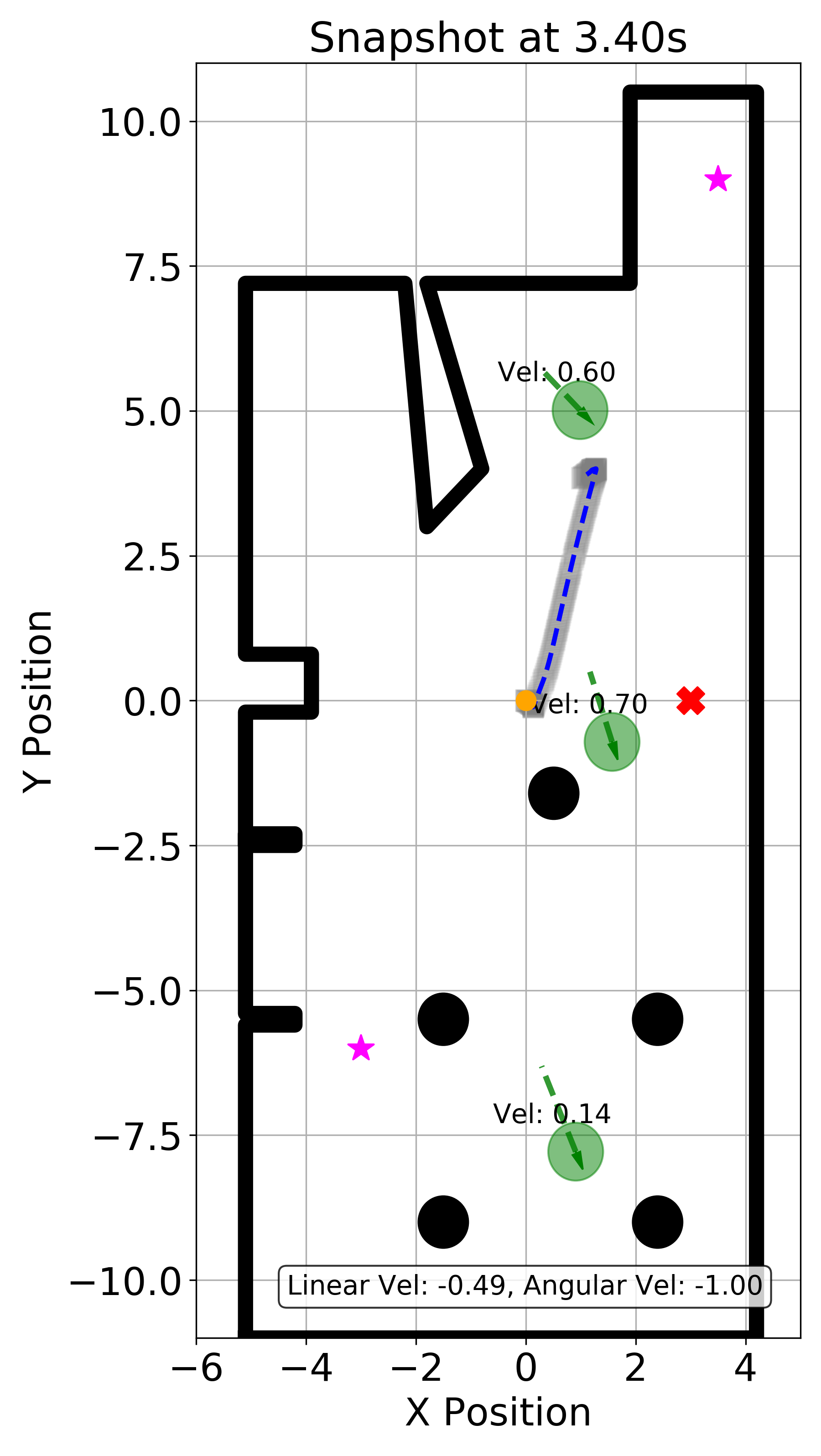
(a)

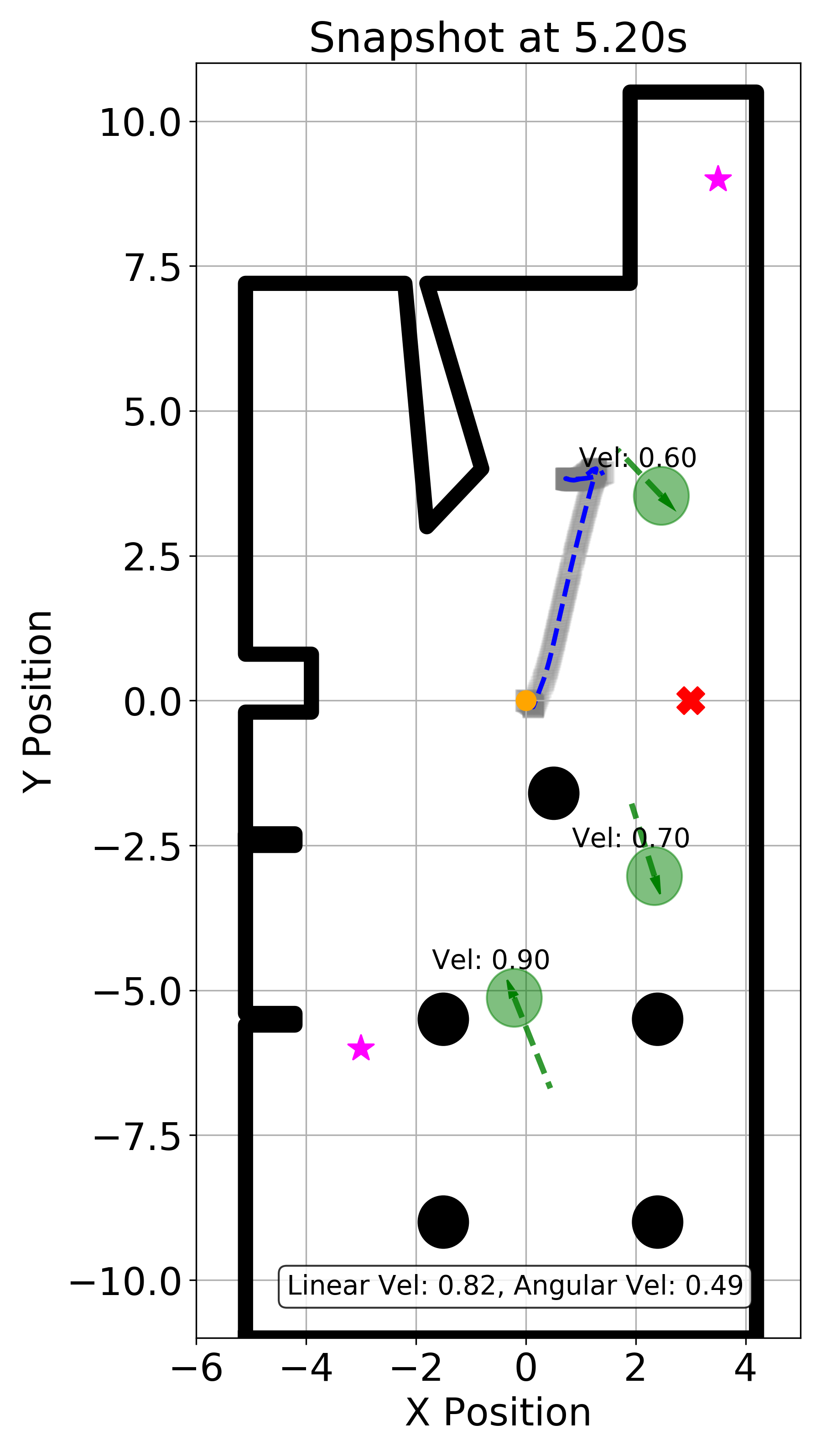
(b)

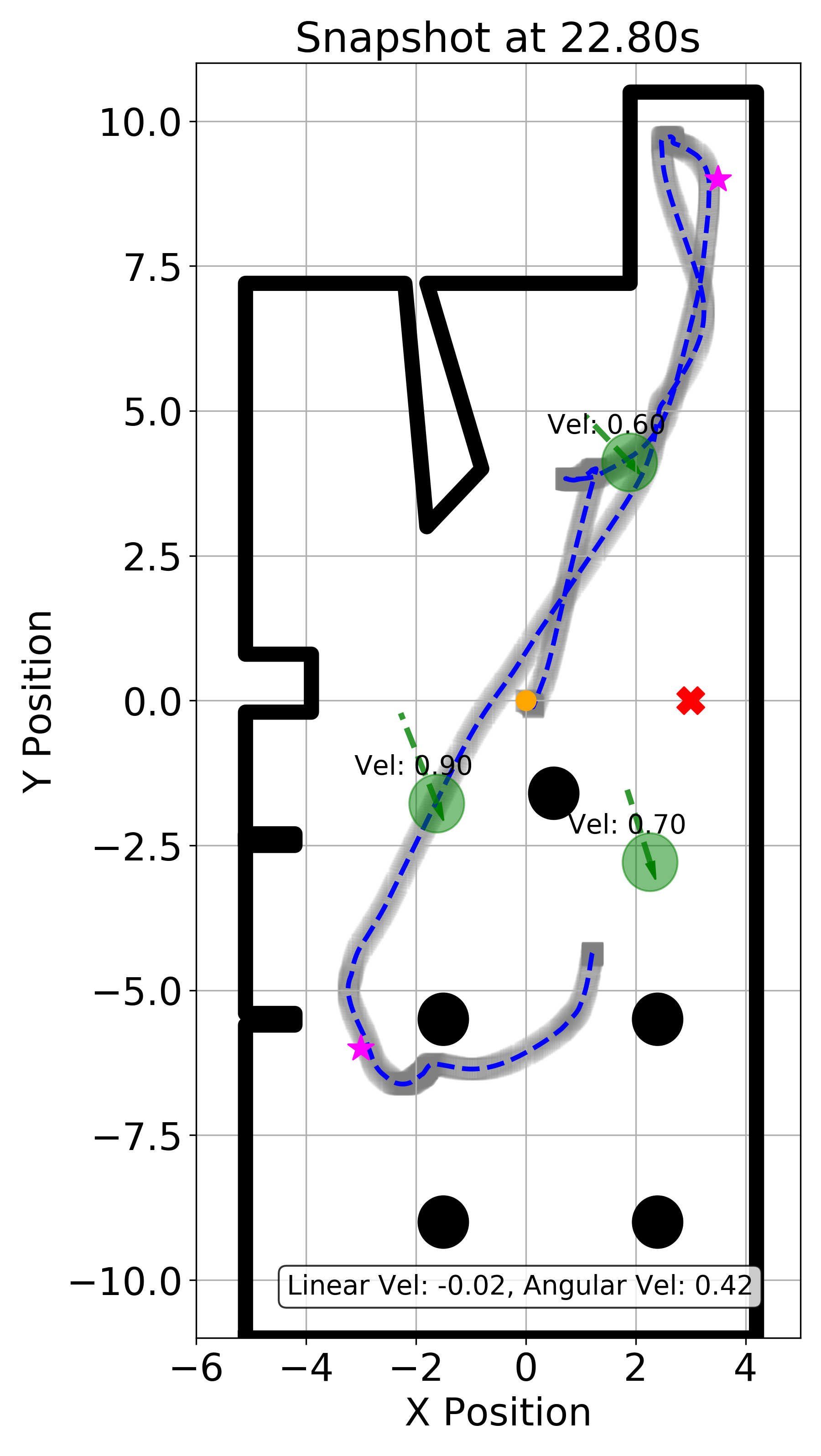
(c)

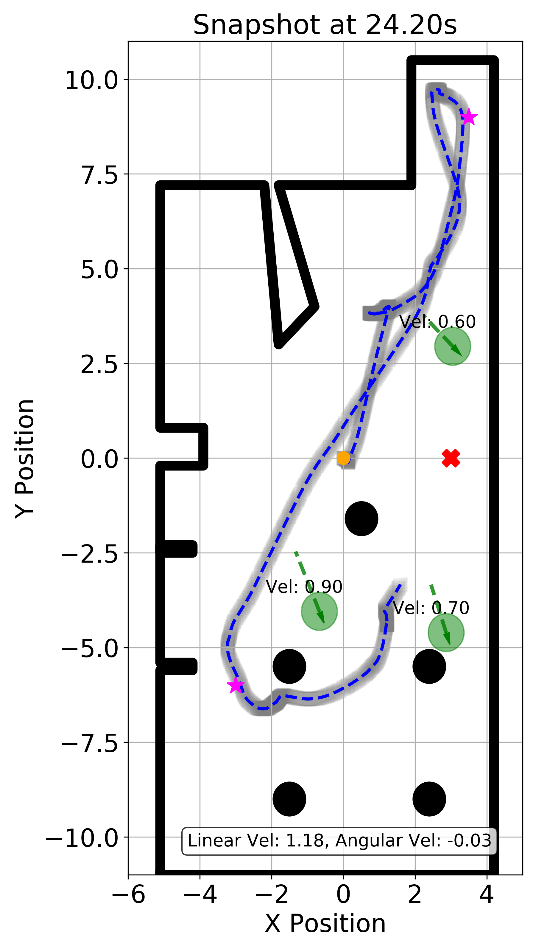
(d)

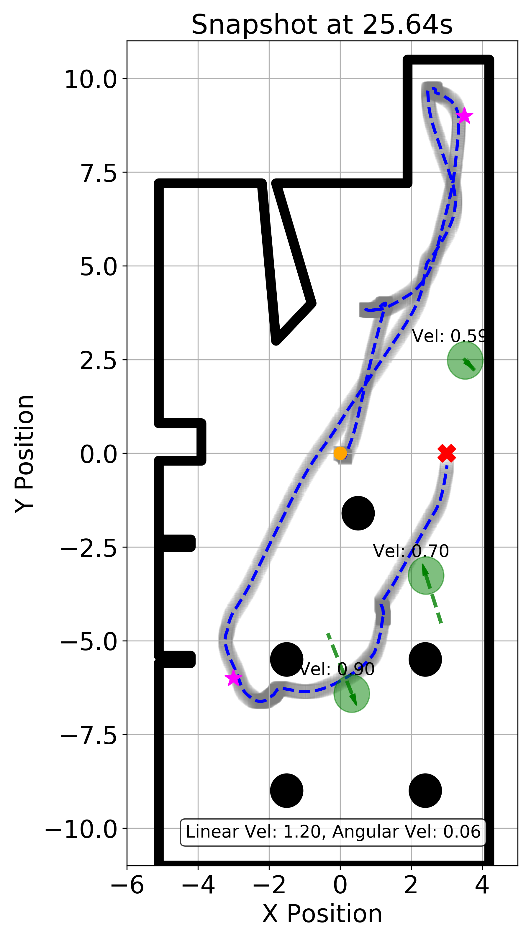
(e)

Figure 9: Snapshots showing safe robot navigation in a simulated dynamic environment with three pedestrians, as depicted in Fig. 5(b). The ground-truth static environment (e.g., walls, table base) is plotted in black. Each pedestrian is represented by a light green circle, with trajectory over the past second and current velocity also displayed. (a) At $t=3.4$s, the robot adjusts its trajectory due to an approaching pedestrian, adopting a defensive maneuver by rotating left ($-1$ rad/s) and moving backwards ($-0.49$m/s). (b) By $t=5.2$s, as the pedestrian clears, the robot accelerates forward ($0.89$m/s) to track its planned path towards the first waypoint. (c) At $t=22.8$s, facing another pedestrian crossing its planned path, the robot stops ($-0.02$m/s) to allow the pedestrian to pass. (d) At $t=24.2$s, the pedestrian has moved away, enabling the robot to resume its course towards the goal. (e) The complete trajectory at $t=25.6$s shows the robot successfully navigated to two waypoints and the final goal, ensuring safety in a dynamically changing environment.

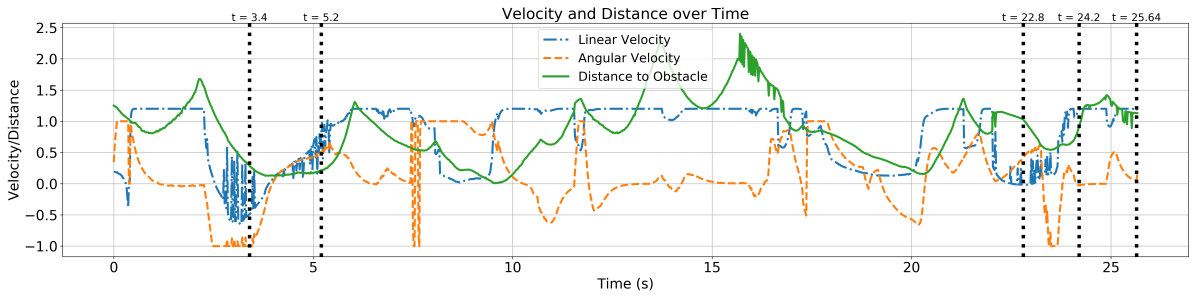
Figure 10: Evaluation of distance to obstacles and robot velocity profile over time in a simulated dynamic environment in Fig. 5(b). The timestamps corresponding to the snapshots in Fig. 9 are indicated with vertical dotted lines, demonstrating the robot’s adaptive responses to dynamic obstacles.

In this section, we evaluate our CLF-DR-CBF QP approach in safe navigation in dynamic environments, cf. Fig. 5(b). Using a social force model (Helbing and Molnar, 1995; Moussaïd et al., 2010), we simulate a scenario within Gazebo that mirrors real-world environments with pedestrians. This simulation aims to reflect the complexities that a mobile robot faces in human-populated areas. Due to limitations of the Gazebo simulator, the position and velocity information of the moving agents are assumed known and provided by Gazebo. In our experiments in Sec. 9.3, these dynamic obstacles are estimated by the onboard sensing. The static elements of the environment are unknown and the robot relies on its LiDAR measurements with noise $\sigma=0.01$ to ensure safety.

In the dynamic simulation shown in Fig. 9, the robot starts at $(0,0)$ and is tasked to sequentially visit two waypoints before reaching a designated goal at $(3,0)$. This task is complicated by the presence of three pedestrians, requiring the robot to dynamically adjust its trajectory to avoid collisions while still aiming to complete its mission efficiently. Note that the $A^{*}$ algorithm operates independently of the pedestrian motion, and the real-time pedestrian avoidance relies on our CLF-DR-CBF QP formulation. This separation emphasizes the role of our approach in ensuring safety in dynamic environments, where pedestrian movement and noisy LiDAR measurements are challenging to consider in the high-level path planning phase.

In Fig. 9(a), at $t=3.4$s, the robot encounters a pedestrian on a collision course with its planned path to the first waypoint at the top right. With our CLF-DR-CBF QP controller, the robot employs a defensive maneuver. This adjustment shows the methodology’s capability to anticipate potential hazards and react accordingly.

As the pedestrian clears the immediate area, the robot resumes its path tracking towards the first waypoint by $5.2$s (Fig. 9(b)). This behavior highlights the efficiency of our approach in balancing mission objectives with the need for safety.

The challenge intensifies at $t=22.8$s when another pedestrian intersects the robot’s planned route (Fig. 9(c)). In response, the robot stops to allow the pedestrian to pass safely. Once the pedestrian has passed, the robot continues its journey towards the goal, as observed at $t=24.2$s (Fig. 9(d)).

The successful completion of the task is shown in Fig. 9(e), where the robot reaches its final goal after safely navigating past all dynamic obstacles at $t=25.64$s. This simulation shows the CLF-DR-CBF QP controller’s ability for robust path tracking and obstacle avoidance in a dynamic environment.

Furthermore, Fig. 10 provides the robot’s distance to obstacles and its velocity profiles over time. The plot confirms that the robot maintains safe distance from the obstacles, including pedestrians, while exhibiting smooth linear and angular velocities.

9.3 Real-World Experiments

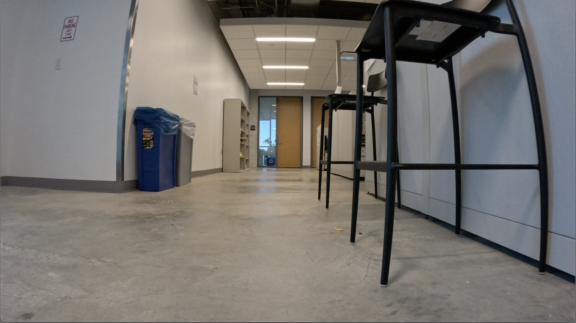
(a)

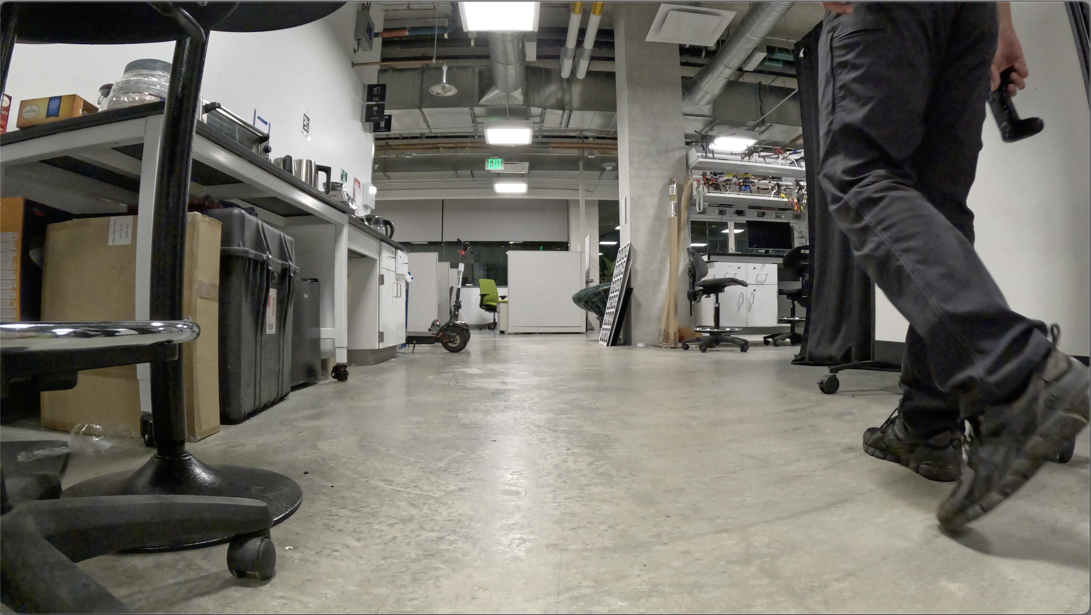
(b)

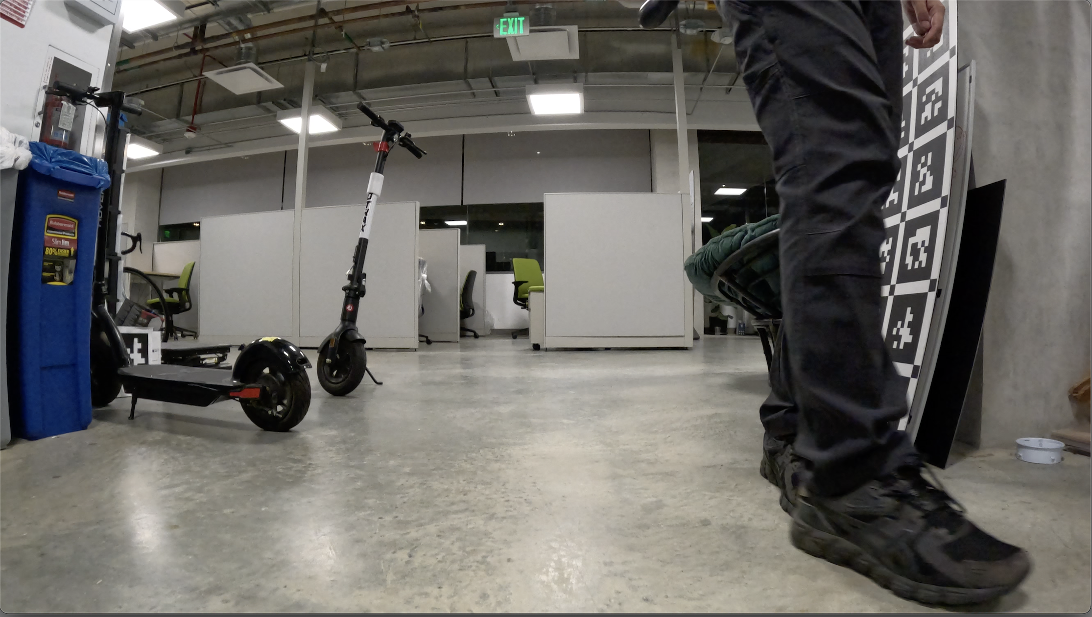
(c)

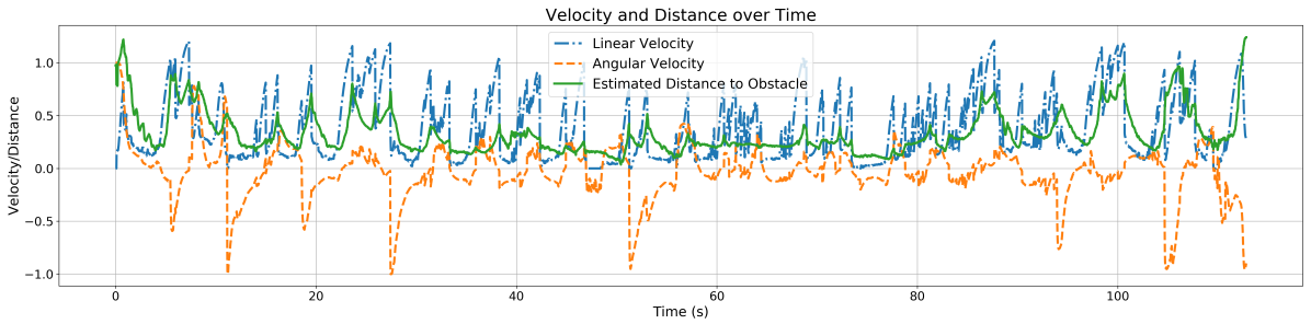
Figure 11: Evaluation of our CLF-DR-CBF QP approach in a real lab environment. The top row shows challenging cases, including navigating around thin chair legs, passing through a narrow passage with pedestrians, and handling an approaching pedestrian. The bottom plot presents the distance to the obstacles and the robot’s velocity profile over time.

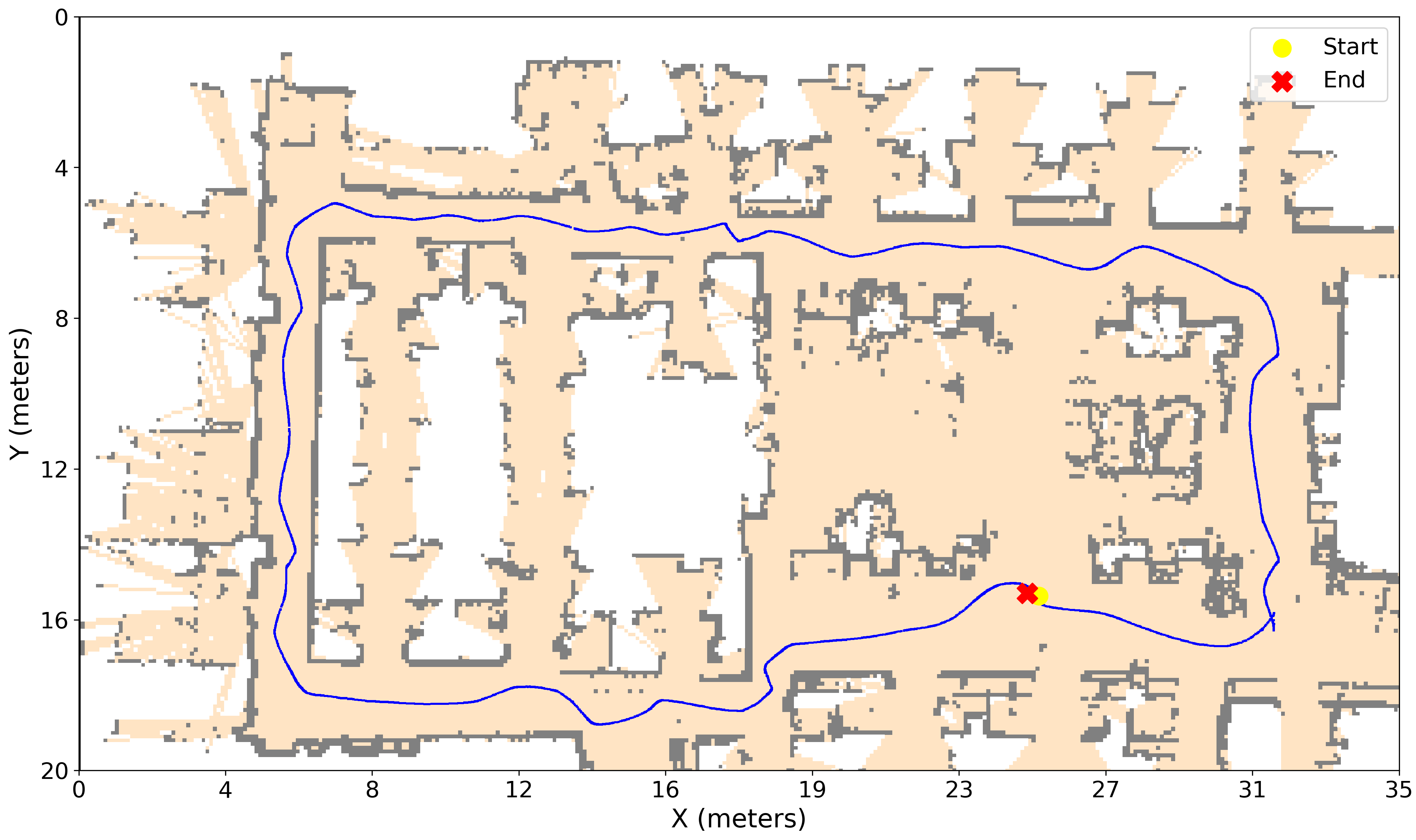
Figure 12: Robot trajectory (blue) and estimated occupancy map (yellow and gray) of the lab environment.

We carried out real-world experiments using a wheeled differential-drive ClearPath Jackal robot (Fig. 1). The robot was equipped with an Intel i7-9700TE CPU with 32GB RAM, an Ouster OS1-32 LiDAR, and a UM7 9-axis IMU, and a velocity controller accepting linear and angular velocity.

We demonstrate the performance of our CLF-DR-CBF QP approach in a cluttered lab environment, where the robot relies solely on LiDAR measurements to navigate around various challenges, such as thin chair legs, narrow passages with pedestrians, and approaching pedestrians. In contrast to the CLF-GP-CBF SOCP formulation, which relies on GP regression to construct CBFs and cannot handle dynamic environments effectively, our CLF-DR-CBF QP formulation maintains safety while solely depending on noisy LiDAR measurements. Fig. 11 shows these challenging scenarios. The bottom plot in Fig. 11 presents the distance to the obstacles and the robot’s velocity profile over time, highlighting the robot’s ability to maintain a safe distance while efficiently navigating towards its goal. For more details, please refer to the accompanying videos on the project webpage.

Fig. 12 depicts the estimated occupancy map and the executed trajectory using our CLF-DR-CBF QP controller. The robot successfully navigates through the cluttered environment, avoiding both static and dynamic obstacles, and reaches its desired goal position.

10 Conclusion

We introduced a novel strategy for ensuring safety of mobile robots navigating autonomously in unknown dynamically changing environments. Our distributionally robust control barrier function formulation leverages sensor measurements directly, eliminating the need for precise CBF estimation, which may be slow and inaccurate in dynamic environments. By combining the DR-CBF with a control Lyapunov function design for path tracking, we developed a CLF-DR-CBF quadratic program that enables safe autonomous navigation for robots with control-affine dynamics. Our approach underscores the efficiency and effectiveness of employing fast sensor-based DR-CBF constraints to handle measurement uncertainty and the complexities of real-world environments. Our experiments demonstrate the ability of our CLF-DR-CBF control method to respond to fast environment changes, while maintaining progress towards a desired navigation goal.

Our results suggest that further exploration into adaptive and sensor-based techniques for robot control may lead to significant progress in deploying reliable autonomous robot systems in the real world. Future work will focus on extending this methodology to more complex robot systems, such as robot arms and humanoids, further bridging the gap between theoretical safety assurances and practical considerations.

We gratefully acknowledge support from ONR Award N00014-23-1-2353, NSF Award CMMI-2044900, and NSF Award CCF-2112665 (TILOS).

References

- Abdi et al. (2023) Abdi H, Raja G and Ghabcheloo R (2023) Safe control using vision-based control barrier function (v-cbf). In: IEEE International Conference on Robotics and Automation (ICRA). pp. 782–788.
- Agrawal et al. (2018) Agrawal A, Verschueren R, Diamond S and Boyd S (2018) A rewriting system for convex optimization problems. Journal of Control and Decision 5(1): 42–60.
- Ames et al. (2019) Ames A, Coogan S, Egerstedt M, Notomista G, Sreenath K and Tabuada P (2019) Control barrier functions: Theory and applications. In: European Control Conference (ECC). pp. 3420–3431.
- Ames et al. (2017) Ames AD, Xu X, Grizzle JW and Tabuada P (2017) Control barrier function based quadratic programs for safety critical systems. IEEE Transactions on Automatic Control 62(8): 3861–3876.
- Aolaritei et al. (2023) Aolaritei L, Fochesato M, Lygeros J and Dörfler F (2023) Wasserstein tube MPC with exact uncertainty propagation. In: IEEE Conference on Decision and Control (CDC). pp. 2036–2041.
- Arslan and Koditschek (2019) Arslan O and Koditschek DE (2019) Sensor-based reactive navigation in unknown convex sphere worlds. The International Journal of Robotics Research 38(2-3): 196–223.
- Artstein (1983) Artstein Z (1983) Stabilization with relaxed controls. Nonlinear Analysis: Theory, Methods & Applications 7: 1163–1173.
- Axelrod et al. (2018) Axelrod B, Kaelbling LP and Lozano-Pérez T (2018) Provably safe robot navigation with obstacle uncertainty. The International Journal of Robotics Research (IJRR) 37(13-14): 1760–1774.
- Borenstein et al. (1991) Borenstein J, Koren Y et al. (1991) The vector field histogram-fast obstacle avoidance for mobile robots. IEEE Transactions on Robotics and Automation 7(3): 278–288.
- Boskos et al. (2023) Boskos D, Cortés J and Martínez S (2023) Data-driven distributionally robust coverage control by mobile robots. In: IEEE Conference on Decision and Control (CDC). pp. 2030–2035.
- Boskos et al. (2024) Boskos D, Cortés J and Martínez S (2024) High-confidence data-driven ambiguity sets for time-varying linear systems. IEEE Transactions on Automatic Control 69(2): 797–812.
- Brooks (1983) Brooks RA (1983) Solving the find-path problem by good representation of free space. IEEE Transactions on Systems, Man, and Cybernetics SMC-13(2): 190–197.
- Chatila and Laumond (1985) Chatila R and Laumond J (1985) Position referencing and consistent world modeling for mobile robots. In: IEEE International Conference on Robotics and Automation (ICRA), volume 2. pp. 138–145.
- Chen et al. (2022) Chen P, Pei J, Lu W and Li M (2022) A deep reinforcement learning based method for real-time path planning and dynamic obstacle avoidance. Neurocomputing 497: 64–75.
- Choi et al. (2023) Choi JJ, Castañeda F, Jung W, Zhang B, Tomlin CJ and Sreenath K (2023) Constraint-guided online data selection for scalable data-driven safety filters in uncertain robotic systems. arXiv preprint arXiv:2311.13824 .
- Chriat and Sun (2023) Chriat AE and Sun C (2023) Wasserstein distributionally robust control barrier function using conditional value-at-risk with differentiable convex programming. arXiv preprint arXiv:2309.08700 .
- Cortés and Egerstedt (2017) Cortés J and Egerstedt M (2017) Coordinated control of multi-robot systems: A survey. SICE Journal of Control, Measurement, and System Integration 10(6): 495–503.
- Coulson et al. (2021) Coulson J, Lygeros J and Dörfler F (2021) Distributionally robust chance constrained data-enabled predictive control. IEEE Transactions on Automatic Control 67(7): 3289–3304.
- Crandall and Lions (1983) Crandall MG and Lions PL (1983) Viscosity solutions of Hamilton-Jacobi equations. Transactions of the American Mathematical Society 277(1): 1–42.
- Dawson et al. (2022) Dawson C, Lowenkamp B, Goff D and Fan C (2022) Learning safe, generalizable perception-based hybrid control with certificates. IEEE Robotics and Automation Letters 7(2): 1904–1911.
- Daş and Murray (2022) Daş E and Murray RM (2022) Robust safe control synthesis with disturbance observer-based control barrier functions. In: IEEE Conference on Decision and Control (CDC). pp. 5566–5573.
- De Lima and Pereira (2013) De Lima DA and Pereira GAS (2013) Navigation of an autonomous car using vector fields and the dynamic window approach. Journal of Control, Automation and Electrical Systems 24: 106–116.
- Desai and Ghaffari (2022) Desai M and Ghaffari A (2022) CLF-CBF based quadratic programs for safe motion control of nonholonomic mobile robots in presence of moving obstacles. In: IEEE/ASME International Conference on Advanced Intelligent Mechatronics (AIM). pp. 16–21.
- Dhiman et al. (2023) Dhiman V, Khojasteh MJ, Franceschetti M and Atanasov N (2023) Control barriers in bayesian learning of system dynamics. IEEE Transactions on Automatic Control 68(1): 214–229.
- Dijkstra (1959) Dijkstra EW (1959) A note on two problems in connexion with graphs. Numerische Mathematik 1: 269–271.
- Dixit et al. (2023) Dixit A, Lindemann L, Wei SX, Cleaveland M, Pappas GJ and Burdick JW (2023) Adaptive conformal prediction for motion planning among dynamic agents. In: Learning for Dynamics and Control Conference. PMLR, pp. 300–314.
- Dudek et al. (1978) Dudek G, Jenkin M, Milios E and Wilkes D (1978) Robotic exploration as graph construction. J. Comput., vol 7(3).
- Emam et al. (2022) Emam Y, Glotfelter P, Wilson S, Notomista G and Egerstedt M (2022) Data-driven robust barrier functions for safe, long-term operation. IEEE Transactions on Robotics 38(3): 1671–1685.
- Esfahani and Kuhn (2018) Esfahani PM and Kuhn D (2018) Data-driven distributionally robust optimization using the Wasserstein metric: performance guarantees and tractable reformulations. Mathematical Programming 171: 115–166.
- Everett et al. (2021) Everett M, Chen YF and How JP (2021) Collision avoidance in pedestrian-rich environments with deep reinforcement learning. IEEE Access 9: 10357–10377.
- Fox et al. (1997) Fox D, Burgard W and Thrun S (1997) The dynamic window approach to collision avoidance. IEEE Robotics Autom. Mag. 4: 23–33.
- Garone and Nicotra (2015) Garone E and Nicotra MM (2015) Explicit reference governor for constrained nonlinear systems. IEEE Transactions on Automatic Control 61(5): 1379–1384.
- Grandia et al. (2021) Grandia R, Taylor AJ, Ames AD and Hutter M (2021) Multi-layered safety for legged robots via control barrier functions and model predictive control. In: IEEE International Conference on Robotics and Automation (ICRA). pp. 8352–8358.
- Hakobyan and Yang (2022) Hakobyan A and Yang I (2022) Distributionally robust risk map for learning-based motion planning and control: A semidefinite programming approach. IEEE Transactions on Robotics 39(1): 718–737.
- Hamdipoor et al. (2023) Hamdipoor V, Meskin N and Cassandras CG (2023) Safe control synthesis using environmentally robust control barrier functions. European Journal of Control 74: 100840. 2023 European Control Conference Special Issue.
- Han et al. (2019) Han L, Gao F, Zhou B and Shen S (2019) Fiesta: Fast incremental euclidean distance fields for online motion planning of aerial robots. In: IEEE/RSJ International Conference on Intelligent Robots and Systems (IROS). pp. 4423–4430.
- Hart et al. (1968) Hart PE, Nilsson NJ and Raphael B (1968) A formal basis for the heuristic determination of minimum cost paths. IEEE Transactions on Systems Science and Cybernetics 4(2): 100–107.
- Helbing and Molnar (1995) Helbing D and Molnar P (1995) Social force model for pedestrian dynamics. Physical Review E 51(5): 4282.
- Herbert et al. (2017) Herbert SL, Chen M, Han S, Bansal S, Fisac JF and Tomlin CJ (2017) FaSTrack: A modular framework for fast and guaranteed safe motion planning. In: IEEE Conference on Decision and Control (CDC). pp. 1517–1522.
- Hoppe et al. (1992) Hoppe H, DeRose T, Duchamp T, McDonald J and Stuetzle W (1992) Surface reconstruction from unorganized points. In: Proceedings of the 19th annual conference on computer graphics and interactive techniques. pp. 71–78.
- Hota et al. (2019) Hota AR, Cherukuri AK and Lygeros J (2019) Data-driven chance constrained optimization under Wasserstein ambiguity sets. In: American Control Conference (ACC). pp. 1501–1506.
- İşleyen et al. (2023) İşleyen A, van de Wouw N and Arslan Ö (2023) Feedback motion prediction for safe unicycle robot navigation. In: IEEE/RSJ International Conference on Intelligent Robots and Systems (IROS). pp. 10511–10518.
- Jiang and Guan (2016) Jiang R and Guan Y (2016) Data-driven chance constrained stochastic program. Mathematical Programming 158: 291–327.
- Keyumarsi et al. (2024) Keyumarsi S, Atman MWS and Gusrialdi A (2024) Lidar-based online control barrier function synthesis for safe navigation in unknown environments. IEEE Robotics and Automation Letters 9(2): 1043–1050.
- Khalil (2002) Khalil HK (2002) Control of nonlinear systems. Prentice Hall, New York, NY.
- Khatib (1986) Khatib O (1986) Real-time obstacle avoidance for manipulators and mobile robots. The International Journal of Robotics Research 5(1): 90–98.
- Khazoom et al. (2022) Khazoom C, Gonzalez-Diaz D, Ding Y and Kim S (2022) Humanoid self-collision avoidance using whole-body control with control barrier functions. In: IEEE International Conference on Humanoid Robots (Humanoids). pp. 558–565.
- Koenig and Howard (2004) Koenig N and Howard A (2004) Design and use paradigms for gazebo, an open-source multi-robot simulator. In: IEEE/RSJ International Conference on Intelligent Robots and Systems (IROS), volume 3. pp. 2149–2154.
- Kohlbrecher et al. (2011) Kohlbrecher S, von Stryk O, Meyer J and Klingauf U (2011) A flexible and scalable slam system with full 3d motion estimation. In: IEEE International Symposium on Safety, Security, and Rescue Robotics. pp. 155–160.
- Lathrop et al. (2021) Lathrop P, Boardman B and Martínez S (2021) Distributionally safe path planning: Wasserstein safe RRT. IEEE Robotics and Automation Letters 7(1): 430–437.
- Li et al. (2023a) Li J, Liu Q, Jin W, Qin J and Hirche S (2023a) Robust safe learning and control in an unknown environment: An uncertainty-separated control barrier function approach. IEEE Robotics and Automation Letters 8(10): 6539–6546.
- Li et al. (2020) Li Z, Arslan Ö and Atanasov N (2020) Fast and safe path-following control using a state-dependent directional metric. In: IEEE International Conference on Robotics and Automation (ICRA). pp. 6176–6182.
- Li et al. (2023b) Li Z, Yi Y, Niu Z and Atanasov N (2023b) EAST: Environment aware safe tracking using planning and control co-design. arXiv preprint arXiv:2310.01363 .
- Lindemann et al. (2023) Lindemann L, Cleaveland M, Shim G and Pappas GJ (2023) Safe planning in dynamic environments using conformal prediction. IEEE Robotics and Automation Letters 8(8): 5116–5123.
- Liu et al. (2023) Liu J, Li M, Huang JK and Grizzle JW (2023) Realtime safety control for bipedal robots to avoid multiple obstacles via clf-cbf constraints. arXiv preprint arXiv:2301.01906 .
- Long et al. (2024) Long K, Cortes J and Atanasov N (2024) Distributionally robust policy and Lyapunov-certificate learning. arXiv preprint arXiv:2404.03017 .
- Long et al. (2022) Long K, Dhiman V, Leok M, Cortés J and Atanasov N (2022) Safe control synthesis with uncertain dynamics and constraints. IEEE Robotics and Automation Letters 7(3): 7295–7302.
- Long et al. (2021) Long K, Qian C, Cortés J and Atanasov N (2021) Learning barrier functions with memory for robust safe navigation. IEEE Robotics and Automation Letters 6(3): 4931–4938.
- Long et al. (2023a) Long K, Yi Y, Cortes J and Atanasov N (2023a) Distributionally robust Lyapunov function search under uncertainty. In: Learning for Dynamics and Control Conference. PMLR, pp. 864–877.
- Long et al. (2023b) Long K, Yi Y, Cortés J and Atanasov N (2023b) Safe and stable control synthesis for uncertain system models via distributionally robust optimization. In: American Control Conference (ACC). pp. 4651–4658.
- Lozano-Perez (1983) Lozano-Perez (1983) Spatial planning: A configuration space approach. IEEE Transactions on Computers C-32(2): 108–120.
- Majd et al. (2021) Majd K, Yaghoubi S, Yamaguchi T, Hoxha B, Prokhorov D and Fainekos G (2021) Safe navigation in human occupied environments using sampling and control barrier functions. In: IEEE/RSJ International Conference on Intelligent Robots and Systems (IROS). pp. 5794–5800.
- Mestres et al. (2023) Mestres P, Allibhoy A and Cortés J (2023) Robinson’s counterexample and regularity properties of optimization-based controllers. arXiv preprint arXiv:2311.13167 .
- Mestres et al. (2024) Mestres P, Long K, Atanasov N and Cortés J (2024) Feasibility analysis and regularity characterization of distributionally robust safe stabilizing controllers. IEEE Control Systems Letters 8: 91–96.
- Moussaïd et al. (2010) Moussaïd M, Perozo N, Garnier S, Helbing D and Theraulaz G (2010) The walking behaviour of pedestrian social groups and its impact on crowd dynamics. PloS one 5(4): e10047.
- Nemirovski and Shapiro (2006) Nemirovski A and Shapiro A (2006) Convex approximations of chance constrained programs. SIAM J. Optim. 17: 969–996.
- Oleynikova et al. (2017) Oleynikova H, Taylor Z, Fehr M, Siegwart R and Nieto J (2017) Voxblox: Incremental 3d Euclidean signed distance fields for on-board MAV planning. In: 2017 IEEE/RSJ International Conference on Intelligent Robots and Systems (IROS). pp. 1366–1373.
- Pfeiffer et al. (2018) Pfeiffer M, Shukla S, Turchetta M, Cadena C, Krause A, Siegwart R and Nieto J (2018) Reinforced imitation: Sample efficient deep reinforcement learning for mapless navigation by leveraging prior demonstrations. IEEE Robotics and Automation Letters 3(4): 4423–4430.
- Prajna and Jadbabaie (2004) Prajna S and Jadbabaie A (2004) Safety verification of hybrid systems using barrier certificates. In: International Workshop on Hybrid Systems: Computation and Control. Springer, pp. 477–492.
- Ramesh et al. (2023) Ramesh SS, Sessa PG, Hu Y, Krause A and Bogunovic I (2023) Distributionally robust model-based reinforcement learning with large state spaces. arXiv preprint arXiv:2309.02236 .
- Ren and Majumdar (2022) Ren AZ and Majumdar A (2022) Distributionally robust policy learning via adversarial environment generation. IEEE Robotics and Automation Letters 7(2): 1379–1386.
- Rimon and Koditschek (1992) Rimon E and Koditschek DE (1992) Exact robot navigation using artificial potential functions. IEEE Transactions on Robotics and Automation 8(5): 501–518.
- Rockafellar and Uryasev (2000) Rockafellar RT and Uryasev S (2000) Optimization of conditional value-at-risk. Journal of Risk 2: 21–41.
- Shafer and Vovk (2008) Shafer G and Vovk V (2008) A tutorial on conformal prediction. Journal of Machine Learning Research 9(3).
- Sontag (1989) Sontag ED (1989) A ‘universal’ construction of Artstein’s theorem on nonlinear stabilization. Systems & Control Letters 13(2): 117–123.
- Van Parys et al. (2016) Van Parys BPG, Kuhn D, Goulart PJ and Morari M (2016) Distributionally robust control of constrained stochastic systems. IEEE Transactions on Automatic Control 61(2): 430–442.
- Wang and Xu (2023) Wang Y and Xu X (2023) Disturbance observer-based robust control barrier functions. In: American Control Conference (ACC). pp. 3681–3687.
- Wu et al. (2023) Wu L, Lee KMB, Le Gentil C and Vidal-Calleja T (2023) Log-gpis-mop: A unified representation for mapping, odometry, and planning. IEEE Transactions on Robotics 39(5): 4078–4094.
- Wu et al. (2021) Wu L, Lee KMB, Liu L and Vidal-Calleja T (2021) Faithful Euclidean distance field from log-gaussian process implicit surfaces. IEEE Robotics and Automation Letters 6(2): 2461–2468.
- Xiao et al. (2022) Xiao W, Wang TH, Chahine M, Amini A, Hasani R and Rus D (2022) Differentiable control barrier functions for vision-based end-to-end autonomous driving. arXiv preprint arXiv:2203.02401 .
- Xie (2021) Xie W (2021) On distributionally robust chance constrained programs with Wasserstein distance. Math. Program. 186: 115–155.
- Yang et al. (2023) Yang S, Pappas GJ, Mangharam R and Lindemann L (2023) Safe perception-based control under stochastic sensor uncertainty using conformal prediction. In: IEEE Conference on Decision and Control (CDC). pp. 6072–6078.
- Yang et al. (2022) Yang W, Gong Z, Huang B and Hong X (2022) Lidar with velocity: Correcting moving objects point cloud distortion from oscillating scanning lidars by fusion with camera. IEEE Robotics and Automation Letters 7(3): 8241–8248.
- Yu et al. (2023) Yu H, Hirayama C, Yu C, Herbert S and Gao S (2023) Sequential neural barriers for scalable dynamic obstacle avoidance. In: IEEE/RSJ International Conference on Intelligent Robots and Systems (IROS). pp. 11241–11248.
- Zhang et al. (2023) Zhang S, Garg K and Fan C (2023) Neural graph control barrier functions guided distributed collision-avoidance multi-agent control. In: Conference on Robot Learning (CoRL). PMLR, pp. 2373–2392.
- Zhang et al. (2024) Zhang Y, Tian G, Wen L, Yao X, Zhang L, Bing Z, He W and Knoll A (2024) Online efficient safety-critical control for mobile robots in unknown dynamic multi-obstacle environments. arXiv preprint arXiv:2402.16449 .
- Zhao et al. (2024) Zhao Y, Yu X, Deshmukh JV and Lindemann L (2024) Conformal predictive programming for chance constrained optimization. arXiv preprint arXiv:2402.07407 .