Risk-Neutral Generative Networks

Abstract

We present a functional generative approach to extract risk-neutral densities from market prices of options. Specifically, we model the log-returns on the time-to-maturity continuum as a stochastic curve driven by standard normal. We then use neural nets to represent the term structures of the location, the scale, and the higher-order moments, and impose stringent conditions on the learning process to ensure the neural net-based curve representation is free of static arbitrage. This specification is structurally clear in that it separates the modeling of randomness from the modeling of the term structures of the parameters. It is data adaptive in that we use neural nets to represent the shape of the stochastic curve. It is also generative in that the functional form of the stochastic curve, although parameterized by neural nets, is an explicit and deterministic function of the standard normal. This explicitness allows for the efficient generation of samples to price options across strikes and maturities, without compromising data adaptability. We have validated the effectiveness of this approach by benchmarking it against a comprehensive set of baseline models. Experiments show that the extracted risk-neutral densities accommodate a diverse range of shapes. Its accuracy significantly outperforms the extensive set of baseline models—including three parametric models and nine stochastic process models—in terms of accuracy and stability. The success of this approach is attributed to its capacity to offer flexible term structures for risk-neutral skewness and kurtosis.

Keywords: Risk-Neutral Density, No-Arbitrage Conditions, Option Pricing, Model Calibration, Generative Machine Learning, Neural Networks

1 Introduction

The risk-neutral pricing theory was developed in the seventies where Cox and Ross, (1976) simplified the option pricing under the Black-Scholes model to an expectation calculation under a risk-neutral measure. This measure integrates the market consensus on future asset prices, adjusted for market risk preferences. Building on these developments, Harrison, Kreps, and Pliska introduced the martingale measure theory. The first Fundamental Theorem of Asset Pricing (FTAP) (Harrison and Kreps,, 1979) states that a market is free of arbitrage opportunities if and only if there exists at least one risk-neutral probability measure, under which the discounted payoffs of securities are martingales. A financial market is arbitrage-free if there is no possibility of constructing a portfolio to generate a sure profit with zero net investment and no risk. The risk-neutral measure effectively adjusts the real-world probabilities of outcomes to reflect a world where all investors are risk-neutral. The second FTAP (Harrison and Pliska,, 1981) further states that the risk-neutral measure is unique if and only if the market is complete. A market is complete if every contingent claim can be replicated exactly by trading in the market, meaning all risks can be perfectly hedged.

Since then, risk-neutral pricing models have become essential tools supporting the modern operation of the options market. Broker-dealers employ them to consistently hedge their option inventories in order to comply with stringent regulatory requirements on net risk exposures. Investors leverage them to identify arbitrage opportunities by calibrating a set of options across different strikes or maturities, assessing non-calibrated options, and exploring discrepancies for profitable investments. The fundamental task of constructing any risk-neutral pricing model ultimately boils down to the extraction of the risk-neutral density from market prices, as the risk-neutral density encapsulates the entirety of information inherent in the traded prices, both completely and exclusively (Cont,, 1997).

The martingale measure theory suggests that when the market is both complete and arbitrage-free, there is exactly one way to price risky assets in a risk-neutral world. It prescribes a self-consistent approach to extract risk-neutral density from market prices. It starts with specifying the dynamics of the discounted value of the underlying asset as a martingale process in the spot risk-neutral measure. This martingale process can be as simple as, for example, a zero-drift SDE, which is then calibrated against market prices through the derived pricing formula of option prices. A model specified as such is arbitrage-free by construction.

Alternatively, researchers have explored the possibility of directly modelling the distribution for the underlying asset at maturity, or the implied volatilities among other quantities of direct interests, without resorting to any dynamics of the underlying. For this approach to work, alternative expressions of no-arbitrage conditions in the same spirit of FTAP need to be imposed during calibration to ensure the model is free from, at least, static arbitrage opportunities (Davis and Hobson,, 2007; Schweizer and Wissel,, 2008; Fengler,, 2009; Föllmer and Schied,, 2011; Cont and Vuletić,, 2023).

Prior methods taking this second approach vary on their degrees of parameterization of the distribution. While higher degrees of parameterization offer structural clarity and computational efficiency, less parameterized specifications are more adaptive to data, particularly when the true distribution has an irregular shape, contains multiple peaks, or has asymmetric heavy tails, but comes at the cost of losing interpretability and increasing computational complexity. However, arbitrage-free is more important than the level of parameterization because it safeguards the model against producing opportunities for riskless profit, which, in theory, should not exist in a complete and efficient market.

What we are after is a generative approach that can balance the parameter interpretability with the data adaptability while rigorously imposing static no-arbitrage conditions. Generative models are notions of machine learning. A model is generative if, given the training data, it can generate new samples from the learned distribution. Prevailing generative models in the machine learning literature typically involve the usage of neural nets. For our purpose, a straightforward thought is also using neural nets to represent the risk-neutral density, for example, following the treatment in the Generative Adversarial Network (GAN) (Goodfellow et al.,, 2014), and letting the calibration process learn the map between option prices and the neural nets’ parameters. However, if the adoption of neural networks is merely for enhancing the adaptability of the distribution to data, it is just another non-parametric specification. This is because neural networks, often viewed as ‘black boxes’, typically lack interpretability.

To reinstall interpretability into the neural-net-based specification, we propose to model the random log-returns on the time-to-maturity continuum as a stochastic curve. Specifically, we assume the log-return curve is a deterministic function of two variables, the standard normal random variable and the time-to-maturity deterministic variable. In our specification, the stochastic curve degenerates to a random scalar associated with the log-return at a fixed maturity time when the time-to-maturity is held constant. Fixing the realized value of the standard normal, the stochastic curve becomes a continuous function of time-to-maturity whose shape is represented by neural nets.

This specification is structurally clear in that it separates the modeling of how the randomness is generated for the stochastic curve from the modeling of the term structure shapes of the location parameter, the scale parameter, and the higher-order moments. It is also data adaptive in that one can use various architectures of neural nets to represent the functional forms of these term structures. The generative feature comes from the fact that the functional form of the log-return stochastic curve, although parameterized by neural nets, is by construction an explicit and deterministic function of the standard normal and the time-to-maturity. This explicitness allows one to generate samples efficiently to compute statistical quantities and to price options at any strikes and maturities.

We call this specification the Risk-Neutral Generative Network (RNGN), and showcase three specific representations: the risk-neutral quantile model (RN-Q) for single maturity calibration, the risk-neutral multi-layer perceptron model (RN-MLP) for multi-maturity calibration, and the risk-neutral double multi-layer perceptrons model (RN-DMLP) for multi-maturity calibration with additional shape complexities. As we make no assumptions of the price dynamics or the distributional families, we shall impose sufficient and (close to) necessary conditions during calibration that are known in the literature, including three sets of inequality constraints on the partial derivatives, two sets of boundary conditions, and one set of pricing bounds.

The empirical experiments show that the extracted density using the RNGN approach can accurately recover a wide range of shapes. It performs outstandingly well against an extensive set of baseline models, including three parametric models and nine stochastic process models. In particular, the RN-DMLP model generally achieves the lowest mean squared error (MSE) on both in-sample and out-of-sample datasets, even in scenarios involving options with extreme moneyness. Comprehensive testing further validates its superior stability. We attribute the success of RN-DMLP to its ability to offer flexible term structures for risk-neutral skewness and kurtosis.

The rest of the paper is organized as follows. Section 2 formulates the problem of risk-neutral distribution extraction and revisits the static no-arbitrage constraints. Section 3 introduces the stochastic curve specification. Section 4 demonstrates the accuracy and stability of the proposed risk-neutral generative network through the simulation and empirical studies. Section 5 provides insights into the higher-order moments of the learned risk-neutral densities. Section 6 concludes the paper.

2 No-Arbitrage Conditions

The time-$t$ prices of European calls and puts on an underlying $S_{t}$, struck at $K$ with time-to-maturity $\tau:=T-t$, are conditional expectations of the discounted payoff under the spot risk-neutral measure $\mathbb{Q}$:

$$\forall r>0,~{}K>0,~{}T\geq t,$$ (1)

$$C(S_{t},K,\tau):=\mathbb{E}^{\mathbb{Q}}[e^{-r\tau}(S_{T}-K)^{+}|S_{t}]=e^{-r\tau}\int_{0}^{\infty}(s-K)^{+}f_{S_{T}}(s)ds,$$

$$P(S_{t},K,\tau):=\mathbb{E}^{\mathbb{Q}}[e^{-r\tau}(K-S_{T})^{+}|S_{t}]=e^{-r\tau}\int_{0}^{\infty}(K-s)^{+}f_{S_{T}}(s)ds,$$

where $f_{S_{T}}(s)$ is the risk-neutral density function of $S_{T}$ at maturity conditional on $S_{t}$, $(\cdot)^{+}$ denotes $\max\{\cdot,0\}$. We assume the discount rate $r$ is a positive constant and there is no dividend payout. Alternatively, we can express (LABEL:eq:payoffF-St) through the log-return $X_{\tau}\coloneqq X_{t:T}=\ln(S_{T}/S_{t})$ and its associated density $q_{X_{\tau}}(x):=S_{t}e^{x}f_{S_{T}}(S_{t}e^{x})$ as

$$C(S_{t},K,\tau) =e^{-r\tau}S_{t}\int_{-\infty}^{+\infty}\bigg{(}e^{x}-S_{t}^{-1}K\bigg{)}^{+}q_{X_{\tau}}(x)dx,$$ (2)

$$P(S_{t},K,\tau) =e^{-r\tau}S_{t}\int_{-\infty}^{+\infty}\bigg{(}S_{t}^{-1}K-e^{x}\bigg{)}^{+}q_{X_{\tau}}(x)dx.$$

Once we know $q_{X_{\tau}}(x)$, we have the density $f_{S_{T}}(s)=\frac{1}{s}\cdot q_{X_{\tau}}(\ln\frac{s}{S_{t}})$ of $S_{T}$ in case it is needed.

We aim to estimate $q_{X_{\tau}}(x)$ from a set of observed prices of calls $\{C_{i}\}_{i=1}^{N_{C}}$ and puts $\{P_{j}\}_{j=1}^{N_{P}}$ by minimizing

$$\frac{1}{N_{C}}\sum_{i=1}^{N_{C}}w^{C}_{i}L(C_{i},\hat{C}_{i})+\frac{1}{N_{P}}\sum_{j=1}^{N_{P}}w^{P}_{j}L(P_{j},\hat{P}_{j}),$$ (3)

where $L(\cdot,\cdot)$ is the loss function, for example, the absolute or relative mean square error (MSE); $\hat{C}_{i}$ and $\hat{P}_{i}$ are the option prices given by the model; $w^{C}_{i}$ and $w^{P}_{i}$ are the regularized weights that may be related to the option liquidity levels and we set $w^{C}_{i}=w^{P}_{i}=1.0$ for simplicity.

In the calibration process, we shall impose the following six conditions that are known to be both sufficient and (close to) necessary (Roper,, 2010, Theorem 2.1) to see what conditions the learned $q_{X_{\tau}}(x)$ should satisfy:

1. $\frac{\partial C}{\partial K}\leq 0$ and $\frac{\partial P}{\partial K}\geq 0$;

2. $\frac{\partial^{2}C}{\partial K^{2}}\geq 0$ and $\frac{\partial^{2}P}{\partial K^{2}}\geq 0$;

3. $\lim_{K\rightarrow\infty}C(S_{t},K,\tau)=C(S_{t},\infty,\tau)=0$ and $\lim_{K\rightarrow 0}P(S_{t},K,\tau)=P(S_{t},0,\tau)=0$;

4. $C(S_{t},K,0)=\left(S_{t}-K\right)^{+}$ and $P(S_{t},K,0)=\left(K-S_{t}\right)^{+}$ when $\tau=0$;

5. $\frac{\partial C}{\partial\tau}\geq 0$ and $\frac{\partial P}{\partial\tau}\geq 0$;

6. $\left(S_{t}-Ke^{-r\tau}\right)^{+}\leq C(S_{t},K,\tau)\leq S_{t}$ and $\left(Ke^{-r\tau}-S_{t}\right)^{+}\leq P(S_{t},K,\tau)\leq Ke^{-r\tau}$.

Constraint 1

The first condition requires the absence of call spread arbitrage among option strikes for any fixed option maturity. From Eqn.(2), we have

$$\frac{\partial C(S_{t},K,\tau)}{\partial K}=-e^{-r\tau}\int_{\ln(K/S_{t})}^{+\infty}q_{X_{\tau}}(x)dx,\quad\forall K>0,~{}\tau\geq 0.$$

For $\frac{\partial C}{\partial K}\leq 0$ to be uniformly non-positive, the integral against $q_{X_{\tau}}(x)$ on the right-hand side needs to be uniformly non-negative, given the negative sign in front of the right-hand side and the fact that the discount factor $e^{-r\tau}$ is positive. Since $q_{X_{\tau}}(x)$ is a density function by construction in our setup where the random variable $X_{\tau}$ will be specified as an explicit function of the standard normal (details to be given in the next section), $q_{X_{\tau}}(x)$ is point-wise non-negative, implying the integral against it is indeed non-negative uniformly. The case for $\frac{\partial P}{\partial K}$ is similar. Therefore, $\frac{\partial C}{\partial K}\leq 0$ and $\frac{\partial P}{\partial K}\geq 0$ always hold in our setup.

Constraint 2

The second condition is to ensure the pricing function free from butterfly spread arbitrage among option strikes for any fixed option maturity. Note that

$$\frac{\partial^{2}C(S_{t},K,\tau)}{\partial K^{2}}=\frac{\partial}{\partial K}\bigg{\{}-e^{-r\tau}\int_{\ln(K/S_{t})}^{+\infty}q_{X_{\tau}}(x)dx\bigg{\}}=\frac{1}{K}e^{-r\tau}q_{X_{\tau}}\bigg{(}\ln\bigg{(}\frac{K}{S_{t}}\bigg{)}\bigg{)},\quad\forall K>0,~{}\tau\geq 0.$$

For the same reason that $q_{X_{\tau}}(\cdot)$ is constructed as a density function which is point-wise non-negative, $\frac{\partial^{2}C(S_{t},K,\tau)}{\partial K^{2}}$ shall be uniformly non-negative. This is also the case for puts. Therefore, $\frac{\partial^{2}C}{\partial K^{2}}\geq 0$ and $\frac{\partial^{2}P}{\partial K^{2}}\geq 0$ always hold.

Constraint 3

The third condition imposes the boundary prices to be zero when the strike price of call options is set to infinity and the strike price of put options is set to zero. It is interpreted as that a put (or call) option has no value if its strike is zero (or infinitely high) because real-world stock prices cannot fall below zero or rise to infinitely high. More specifically, $\max(s-K,0)|_{K=+\infty}=0$ holds for the call case and $\max(K-s,0)|_{K=0}=0$ holds for the put case in Eqn.(LABEL:eq:payoffF-St), where $s$ is any possible realized value of $S_{T}$. Therefore, this constraint is satisfied in our setup.

Constraint 4

The fourth one sets price conditions on the zero time-to-maturity boundary. It is equivalent to requiring the random variable $X_{\tau}$ is degenerate, i.e., it almost surely takes a specific value, $X_{0}$, as the option’s maturity is infinitely close to the current calendar time. In other words, its density $q_{X_{\tau}}(x)$ becomes a Dirac delta function,

$$\lim_{\tau\downarrow 0}q_{X_{\tau}}(x)=\delta(x-X_{0}),~{}\textrm{where}\ X_{0}:=\lim_{t\leftarrow T}\ln(S_{T}/S_{t})=0.$$

The Dirac delta function $\delta(x-X_{0})$ is zero everywhere except at $x=X_{0}$. It has the property that the integral of the Dirac delta function against any continuous test function $\phi(x)$ picks out the value of the test function at $X_{0}$: $\int_{\mathbb{R}}\phi(x)\delta(x-X_{0})dx=\phi(X_{0})$.

For $q_{X_{\tau}}(x)$ to be a Dirac delta function, it means $X_{\tau}$ takes on the value $X_{0}$ with probability one almost surely,

$$\mathbb{P}(X_{\tau}=X_{0})=\int_{\mathbb{R}}\delta(x-X_{0})dx=1,~{}\textrm{where}\ X_{0}=0.$$

Therefore, option prices on the zero time-to-maturity boundary are equal to their payoffs,

$$C(S_{t},K,0)=\lim_{\tau\downarrow 0}e^{-r\tau}S_{t}\int_{\mathbb{R}}\bigg{(}e^{x}-S_{t}^{-1}K\bigg{)}^{+}\delta(x)dx=(S_{t}-K)^{+},$$

$$P(S_{t},K,0)=\lim_{\tau\downarrow 0}e^{-r\tau}S_{t}\int_{\mathbb{R}}\bigg{(}S_{t}^{-1}K-e^{x}\bigg{)}^{+}\delta(x)dx=(K-S_{t})^{+}.$$

In the next section, we shall show that our specifications for $X_{\tau}$ have made sure that $X_{\tau}$ indeed takes on the value $X_{0}$ with probability one as $\tau$ approaches the zero boundary.

Constraint 5

The fifth condition is equivalent to the absence of calendar spread arbitrage between adjacent maturities for any fixed strike. It demands that the pricing functions, i.e. (2), should be monotonically increasing as the time-to-maturity extends, upon fixing the rest of other contractual and model parameters. It reflects the economic principle that an optionality should be more valuable if it gives the holder a higher chance to be potentially more profitable. In the case of a call (or put) option, a longer maturity implies there is more time, hence a higher probability, for the underlying stock to surpass (or fall below) a given threshold. We shall impose this condition as a soft constraint through a regularization term when calibrating the model, as detailed in Section 3.

Constraint 6

The sixth condition imposes upper and lower bounds on the prices of European options. Together with the non-negativity of option prices, these pricing bounds are direct consequences of assuming the following equality (holds uniformly for any time-to-maturity):

$$\ln\mathbb{E}^{\mathbb{Q}}[e^{X_{\tau}}]=r\tau,\quad\forall\tau>0.$$ (4)

It is equivalent to requiring that the present value of the stock price at any future time, as a conditional expectation under the spot risk-neutral measure, equals the current stock price,

$$\mathbb{E}_{t}^{Q}[S_{T}]=S_{t}e^{r(T-t)},\quad\forall T>t.$$ (5)

The argument is as follows. First, if $\mathbb{E}_{t}^{Q}[S_{T}]=S_{t}e^{r(T-t)}$ holds for all $T>t$, then the put-call parity holds,

$$\quad C(S_{t},K,\tau)-P(S_{t},K,\tau)=e^{-r\tau}\int_{0}^{+\infty}\big{[}(s-K)^{+}-(K-s)^{+}\big{]}f_{S_{T}}(s)ds$$

$$=e^{-r\tau}\int_{0}^{+\infty}(s-K)f_{S_{T}}(s)ds=e^{-r\tau}\int_{0}^{+\infty}sf_{S_{T}}(s)ds-e^{-r\tau}\int_{0}^{+\infty}Kf_{S_{T}}(s)ds$$

$$=e^{-r\tau}\mathbb{E}_{t}^{Q}[S_{T}]-Ke^{-r\tau}=S_{t}-Ke^{-r\tau},\quad\forall\tau>0,~{}K>0.$$

The lower bound of calls is obtained by applying the put-call parity and using the fact that option prices are non-negative,

$$C(S_{t},K,\tau)=P(S_{t},K,\tau)+S_{t}-Ke^{-r\tau}\geq S_{t}-Ke^{-r\tau}\ \textrm{and}\ C(S_{t},K,\tau)\geq 0.$$

Together, we have calls bounded below as $C(S_{t},K,\tau)\geq(S_{t}-Ke^{-r\tau})^{+},~{}\forall\tau>0,~{}K>0$.

The upper bound of calls is the consequence of putting Contraint 1, i.e. $\frac{\partial C}{\partial K}\leq 0$, together with the equality we assume to hold, i.e. $\mathbb{E}_{t}^{Q}[S_{T}]=S_{t}e^{r(T-t)},~{}\forall T>t$,

$$C(S_{t},K,\tau)\leq C(S_{t},0,\tau)\ \textrm{where}\ C(S_{t},0,\tau)=e^{-r\tau}\int_{0}^{+\infty}sf_{S_{T}}(s)ds=e^{-r\tau}\mathbb{E}_{t}^{Q}[S_{T}]=S_{t}.$$

Therefore, calls are bounded above as $C(S_{t},K,\tau)\leq C(S_{t},0,\tau)=S_{t},~{}\forall K>0,~{}\tau>0$.

In the case of put options, the argument is similar. First, we already know from the upper bound of calls that $C(S_{t},K,\tau)-S_{t}\leq 0$. Therefore, the puts are bounded above by $Ke^{-r\tau}$ from the put-call parity because $P(S_{t},K,\tau)=Ke^{-r\tau}+C(S_{t},K,\tau)-S_{t}\leq Ke^{-r\tau}$. Meanwhile, by the non-negativity of option prices, both $P(S_{t},K,\tau)\geq 0$ and $P(S_{t},K,\tau)=Ke^{-r\tau}+C(S_{t},K,\tau)-S_{t}\geq Ke^{-r\tau}-S_{t}$ should hold. Put them together and we have the puts bounded below by $(Ke^{-r\tau}-S_{t})^{+}$.

Rechecking the equality $\mathbb{E}_{t}^{Q}[S_{T}]=S_{t}e^{r(T-t)}$, or equivalently, $C(S_{t},0,\tau)=S_{t}$, we argue that it should hold in a rational market because a call option with a zero strike will always be exercised, resulting in a payoff $S_{T}$. This is equivalent to possessing the underlying asset directly.

To summarize, Constraints 1–4 collectively require that the log-return random variable $X_{\tau}$ has a density degenerating to the Dirac delta function on the zero time-to-maturity boundary. Constraint 5 further regulates the density behavior of $X_{\tau}$ along the time-to-maturity dimension to ensure that options prices are non-decreasing functions of time-to-maturity. Constraint 6 requires that the expected future stock price at any future time should equal the current stock price grown at the risk-free rate.

3 Model Specification

At different option maturity times, the log-returns $X_{\tau}=\ln(S_{T}/S_{t})$ are scalar random variables, characterized by their individual marginal distributions. Put together, they form a random vector $[X_{\tau_{1}},\cdots,X_{\tau_{n}}]^{\top}$, characterized by their joint distribution. When the time-to-maturity $\tau$ is continuous, the random vector becomes a stochastic curve $X_{\tau}$.

Our specification begins by assuming the log-return stochastic curve $X_{\tau}=\ln(S_{T}/S_{t})$ on the time-to-maturity continuum is a function of two variables, the standard normal random variable $Z$ and the time-to-maturity deterministic variable $\tau$,

$$X_{\tau} :=X(Z,\tau)=\mu(\tau)+\sigma(\tau)\cdot Z\cdot G(Z,\tau),\quad Z\sim\mathbb{N}(0,1),~{}\tau\in\mathbb{R}^{+},$$ (6)

$$X_{0} :=\lim_{t\leftarrow T}\ln(S_{T}/S_{t})=0,$$

where $\mu(\cdot),~{}\sigma(\cdot),~{}G(\cdot,\cdot)$ are deterministic functions, either in closed forms or parameterized by neural nets with the Softplus activation function $\ln\left(1+\exp(x)\right)$.

This specification is functionally parsimonious. Holding $\tau$ constant, $X(Z,\tau)$ degenerates to a random scalar, representing the log-return at a specific time-to-maturity. The map in the first variable $Z\mapsto X(Z,\cdot)$ is responsible for generating the randomness of $X(Z,\cdot)$ from that of the standard normal $Z$. Meanwhile, the map in the second variable $\tau\mapsto X(\cdot,\tau)$ is responsible for capturing the variations in the shape of the log-return’s distribution along the time-to-maturity dimension.

In the meantime, this specification remains structurally interpretable without sacrificing its adaptability to data. In particular, $\mu(\tau)$ models the location term structure of the log-returns analogous to the mean, $\sigma(\tau)$ represents the scale term structure analogous to the volatility, and through $G(\cdot,\tau)$ the term structures of higher-order moments such as skewness and kurtosis. One can set $Z\mapsto G(Z,\cdot)$ as simple as the identity map $G(Z,\cdot)\equiv 1$, yielding normal distributions for $X_{\tau}\sim\mathbb{N}(\mu(\tau),\sigma^{2}(\tau))$, or as flexible as represented by neural nets to capture any non-Gaussian distributional properties of the financial data (Cont,, 2001), such as having irregular shapes, containing multiple peaks, or exhibiting asymmetric heavy tails. The three term structure maps, $\tau\mapsto\mu(\tau)$, $\tau\mapsto\sigma(\tau)$, and $\tau\mapsto G(\cdot,\tau)$, can either be in closed forms for simplicity, e.g. $\sigma(\tau)=\sigma\sqrt{\tau}$, or be parameterized by neural nets to cater to the real-world complexities of variations in the data distribution.

In addition, this specification is generative by construction in that the functional form of $X(Z,\tau)$ is an explicit and deterministic function of the standard normal. For calibration, sample averaging shall approximate well the option prices,

$$\hat{C}(S_{t},K,\tau)=e^{-r\tau}S_{t}\cdot\frac{1}{N}\sum_{n=1}^{N}\left(e^{X(Z_{n},\tau)}-S_{t}^{-1}K\right)^{+},$$ (7)

$$\hat{P}(S_{t},K,\tau)=e^{-r\tau}S_{t}\cdot\frac{1}{N}\sum_{n=1}^{N}\left(S_{t}^{-1}K-e^{X(Z_{n},\tau)}\right)^{+}.$$

Here $Z_{n}$ is a sample of $Z$, and thereby $X(Z_{n},\tau)$ is a sample of the log-return $X_{\tau}$. Once the model parameters are learned, computing statistics of interest is also straightforward. The only simulation needed is a set of standard normal samples.

Finally, there exists a continuous density for $X(Z,\tau)$ specified by Eqn.(6), when $\mu(\cdot)$, $\sigma(\cdot)$, and $G(\cdot,\cdot)$ in Eqn.(6) are represented by multi-layer perceptrons (MLPs) with the Softplus activation. If they are such MLPs, they consist of a finite number of simple mathematical operations, therefore $X(\cdot,\tau)$ is a piecewise (strictly) monotonic function when fixing $\tau$. Applying the general form of the change-of-variable formula (Casella and Berger,, 2024, Theorem 2.1.8), we can conclude that the random variable $X(Z,\tau)$ has a continuous density.

In the upcoming subsections, we showcase three different specifications for $X_{\tau}$, one for single maturity calibration, one for multi-maturity calibration, and one for multi-maturity calibration with additional shape complexities. For these three particular specifications, Constraints 1–4 hold by construction; Constraint 5 shall be enforced as inequality constraints and Constraint 6 as an equality constraint requiring

$$\ln\mathbb{E}^{\mathbb{Q}}\Big{[}\exp\Big{(}\mu(\tau)+\sigma(\tau)\cdot Z\cdot G(Z,\tau)\Big{)}\Big{]}=r\tau,\quad\forall\tau>0.$$ (8)

3.1 Single Maturity

When there is only one maturity, there is no notion of term structure. The stochastic curve $X_{\tau}$ becomes a random scalar. We can drop the subscript $\tau$ in $X_{\tau}$ and set

$$\mu(\tau):=\mu,~{}~{}\sigma(\tau):=\sigma,~{}~{}G(Z,\tau):=G(Z).$$ (9)

If we assume $G(Z)=\frac{u^{Z}}{A}+\frac{v^{-Z}}{A}+1$, we have the log-return $X$ taking the following form,

$$X=\mu+\sigma Z\left(\frac{u^{Z}}{A}+\frac{v^{-Z}}{A}+1\right),$$ (10)

where $\mu$ and $\sigma$ are the location and scale parameters; $u\geq 1$ controls the right tail and $v\geq 1$ controls the left tail; $A$ is a positive constant. Setting $u=v=1$ turns $X$ into a normal distribution as $G(Z)$ becomes a constant. This specification recovers the model introduced in Yan et al., (2019), which was proposed to capture the asymmetric heavy tail nature of asset returns, motivated by the parsimonious heavy-tailed quantile function ideas (Yan et al.,, 2018; Wu and Yan,, 2019).

Given the model parameters $\left\{\mu,\sigma,u,v\right\}$, the market observables $\left\{S_{t},r\right\}$, and the contractual parameters $\left\{K^{C},\tau\right\}$ or $\left\{K^{P},\tau\right\}$ for the call or the put, we obtain the model prices by drawing $N$ standard normal samples $\{Z_{n}\}$ and averaging the discounted payoffs,

$$\hat{C}_{Q}=\frac{1}{N}\sum_{n=1}^{N}e^{-r\tau}S_{t}\left(e^{X(Z_{n})}-S_{t}^{-1}K^{C}\right)^{+},$$ (11)

$$\hat{P}_{Q}=\frac{1}{N}\sum_{n=1}^{N}e^{-r\tau}S_{t}\left(S_{t}^{-1}K^{P}-e^{X(Z_{n})}\right)^{+},$$

where

$$X(Z_{n})=\mu+\sigma Z_{n}\left(\frac{u^{Z_{n}}}{A}+\frac{v^{-Z_{n}}}{A}+1\right).$$ (12)

The log-return as specified in Eqn.(10) always attains a density, therefore Constraints 1-3 shall hold. Constraints 4 and 5 are not applicable for the single maturity case as they concern price behaviors with changing time-to-maturity. For Constraint 6, we drive from Eqn.(8) that the model parameters $\left\{\mu,\sigma,u,v\right\}$ should satisfy the following equality as a hard constraint at a fixed $\tau$,

$$\mu+\ln\left[\frac{1}{N}\sum^{N}_{n=1}\exp\Big{(}\sigma Z_{n}\big{(}\frac{u^{Z_{n}}}{A}+\frac{v^{-Z_{n}}}{A}+1\big{)}\Big{)}\right]=r\tau,$$ (13)

which is equivalent to Eqn.(8) after replacing the expecation by the sample average. Therefore, one only needs to calibrate the three parameters $\sigma,u,v$.

We call this specification, Eqns.(LABEL:eq:pricing_formula-Q)–(13), the RN-Q (Risk-Neutral Quantile Model) and shall use it as the base model for later studies.

3.2 Multiple Maturities

When there are multiple maturities to calibrate, we shall set the functions $\mu(\tau)$, $\sigma(\tau)$, and $G(Z,\tau)$ as,

$$\mu(\tau):=r\cdot\tau\cdot G^{\mu}(\tau;\theta^{\mu}),$$ (14)

$$\sigma(\tau):=\sigma\sqrt{\tau},$$

$$G(Z,\tau):=G^{Z}(Z;\theta^{Z})+G^{\tau}(\tau;\theta^{\tau})+1,$$

where $G^{\mu},~{}G^{Z},~{}G^{\tau}$ are MLP neural nets with the Softplus activation, parameterized by $\theta^{\mu},~{}\theta^{Z},~{}\theta^{\tau}$; $Z$ and $\tau$ are the same standard normal variable and the time-to-maturity variable as before. The resulting log-return stochastic curve is as follows,

$$X_{\tau}:=X(Z,\tau;\theta^{M})=r\tau G^{\mu}(\tau;\theta^{\mu})+\sigma\sqrt{\tau}Z[G^{Z}(Z;\theta^{Z})+G^{\tau}(\tau;\theta^{\tau})+1],\quad\forall\tau>0,$$ (15)

$$X_{0}:=X(Z,\tau;\theta^{M})|_{\tau=0}=0.$$

Note that the above specifications are by no means the only choice. For example, if a stochastic mean is deemed necessary, one can let $\mu(\tau)$ depend on $Z^{\prime}$ in addition to $\tau$, e.g. $\mu(Z^{\prime},\tau)=r\tau G^{\mu}(Z^{\prime},\tau;\theta^{\mu})$, where $Z^{\prime}$ can be the same as, independent of, or partially correlated with the standard normal $Z$ used in $G(Z,\cdot)$. Similarly, if the volatility term structure in the data deviates from the square root law, additional shape adjustments can be made to $\sigma\sqrt{\tau}$, using either parametric or non-parametric forms. For example, $\sigma(\tau)=\sigma\sqrt{\tau}f(\tau)$.

We impose an additive structure in the function $G(Z,\tau)$, where the first component $G^{Z}(Z;\theta^{Z})$ depends only on $Z$ as the input, and $G^{\tau}(\tau;\theta^{\tau})$ depends only on $\tau$ as the input. This structure facilitates the derivation of the first-order partial derivatives with respect to the variables $Z$ and $\tau$ when learning the parameters of the neural nets.

We shall term this specification the RN-MLP model (Risk-Neutral Generative Network with Multi-Layer Perceptron), under which the pricing formulas are as follows, $\forall\tau>0$,

$$\hat{C}_{M} =S_{t}e^{-r\tau}\frac{1}{N}\sum_{n=1}^{N}\bigg{(}e^{X(Z_{n},\tau;\theta^{M})}-S_{t}^{-1}K^{C}\bigg{)}^{+},$$ (16)

$$\hat{P}_{M} =S_{t}e^{-r\tau}\frac{1}{N}\sum_{n=1}^{N}\bigg{(}S_{t}^{-1}K^{P}-e^{X(Z_{n},\tau;\theta^{M})}\bigg{)}^{+},$$

where $Z_{n}$ is the $n$-th sample of $Z$ and $\theta^{M}=\{\theta^{\mu},\theta^{Z},\theta^{\tau},\sigma\}$ is the trainable parameter set.

From the discussions on the density before, we know (15) attains a density, therefore Constraints 1–3 hold. We let the location term $\mu(\tau)=r\tau G^{\mu}(\tau;\theta^{\mu})$ and the scale term $\sigma(\tau)=\sigma\sqrt{\tau}$ depend on $\tau$ explicitly to ensure $X_{\tau}$ does indeed degenerate to $0$ at $\tau=0$ to satisfy Constraint 4. In Proposition 1, we introduce conditions under which the model prices $\hat{C}_{M}$ and $\hat{P}_{M}$, given by Eqn.(16), satisfy Constraints 5 and 6, therefore are free from static arbitrage.

Proposition 1.

Let the log-return curve $X_{\tau}$ follow the specification given by Eqn.(15). The associated option prices $\hat{C}_{M}$ and $\hat{P}_{M}$ in Eqn.(16) are free from static arbitrage if and only if 1) $\tilde{J}^{\tau}_{C}(\tau,K^{C},\theta^{M})\geq 0$, 2) $\tilde{J}^{\tau}_{P}(\tau,K^{P},\theta^{M})\geq 0$, and 3) $J^{\mu}_{M}(\tau,\theta^{M})=0$ where $\theta^{M}=\{\theta^{\mu},\theta^{Z},\theta^{\tau},\sigma\}$ and

$$\tilde{J}^{\tau}_{C}(\tau,K^{C},\theta^{M}) \coloneqq\frac{1}{N}\sum_{n=1}^{N}\mathbb{I}_{\{e^{X(Z_{n},\tau;\theta^{M})}\geq\frac{K^{C}}{S_{t}}\}}\left[\left({\partial_{\tau}X(Z_{n},\tau;\theta^{M})}-r\right)e^{X(Z_{n},\tau;\theta^{M})}+r\frac{K^{C}}{S_{t}}\right],$$ (17)

$$\tilde{J}^{\tau}_{P}(\tau,K^{P},\theta^{M}) \coloneqq\frac{1}{N}\sum_{n=1}^{N}\mathbb{I}_{\{e^{X(Z_{n},\tau;\theta^{M})}\leq\frac{K^{P}}{S_{t}}\}}\left[\left(r-{\partial_{\tau}X(Z_{n},\tau;\theta^{M})}\right)e^{X(Z_{n},\tau;\theta^{M})}-r\frac{K^{P}}{S_{t}}\right],$$

$$J^{\mu}_{M}(\tau,\theta^{M}) \coloneqq\left|r\tau\left(G^{\mu}(\tau;\theta^{\mu})-1\right)+\ln\left(\frac{1}{N}\sum_{n=1}^{N}e^{\sigma\sqrt{\tau}\cdot Z_{n}\cdot[G^{Z}(Z_{n};\theta^{Z})+G^{\tau}(\tau;\theta^{\tau})+1]}\right)\right|^{2}.$$

The proof can be found in Appendix A.1.

Consequently, to train the RN-MLP model, we optimize the following objective:

$$\underset{\theta^{M}}{\text{min}} \mathcal{L}_{M}:=\frac{1}{N_{C}}\sum_{i=1}^{N_{C}}L(C_{i},\hat{C}_{i})+\frac{1}{N_{P}}\sum_{{j}=1}^{N_{P}}L(P_{j},\hat{P}_{j}),$$ (18)

subject to $$~{}\tilde{J}^{\tau}_{C}(\tau,K^{C},\theta^{M})\geq 0,~{}\tilde{J}^{\tau}_{P}(\tau,K^{P},\theta^{M})\geq 0,~{}J^{\mu}_{M}(\tau,\theta^{M})=0.$$

$L$ is the loss function, for example, either the absolute or the relative mean square error (MSE); $\{C_{i},P_{j}\}$ are the observed market prices of options; and $\{\hat{C}_{i},\hat{P}_{j}\}$ are the model prices. In practice, the above constrained optimization problem is rather difficult to solve with multi-layer neural networks. We can reformulate the problem (18) as an unconstrained one through penalized relaxation,

$$\underset{\theta^{M}}{\text{min}}\quad\mathcal{L}_{M} :=\frac{1}{N_{C}}\sum_{i=1}^{N_{C}}L(C_{i},\hat{C}_{i})+\frac{1}{N_{P}}\sum_{{j}=1}^{N_{P}}L(P_{j},\hat{P}_{j})+\lambda\cdot J(\theta^{M}),$$ (19)

$$J(\theta^{M}) :=\sum_{\{\tau,K^{C}\}}\left(-\tilde{J}^{\tau}_{C}(\tau,K^{C},\theta^{M})\right)^{+}$$

$$+\sum_{\{\tau,K^{P}\}}\left(-\tilde{J}^{\tau}_{P}(\tau,K^{P},\theta^{M})\right)^{+}+\sum_{\{\tau\}}J_{M}^{\mu}(\tau,\theta^{M}).$$

$J(\theta^{M})$ is the penalty term and $\lambda$ is the regularization hyper-parameter which can be set to one in the experiments.

3.3 Additional Shape Flexibilities

The RN-MLP model can flexibly model the log-returns with complex risk-neutral densities because MLP is a universal approximator (Hornik et al.,, 1989; Baldi and Hornik,, 1989). However, sometimes the log-return exhibits a bi-modal or multi-modal distribution (e.g., see Orosi, (2015) and Schmitt and Westerhoff, (2017)). We showcase how to extend the single RN-MLP specification into a mixture of two RN-MLPs to allow additional shape flexibilities,

$$X_{\tau}:=X(Z,\tau;\theta^{dM})=\alpha\cdot X_{1}(Z,\tau;\theta^{M}_{1})+(1-\alpha)\cdot X_{2}(Z,\tau;\theta^{M}_{2}),\quad\forall\tau>0,$$ (20)

$$X_{0}:=X(Z,\tau;\theta^{dM})|_{\tau=0}=0,$$

where $\alpha\in\mathbb{R}$, which is not limited in $[0,1]$, and $X_{i},~{}i=1,2$ share the same structure as that of RN-MLP in Eqn.(15),

$$X_{i}(Z,\tau;\theta_{i}^{M})=r\tau G_{i}^{\mu}(\tau;\theta_{i}^{\mu})+\sigma_{i}Q_{i}(Z,\tau;\theta^{\sigma}_{i}),$$ (21)

with $$Q_{i}(Z,\tau;\theta^{\sigma}_{i})=\sqrt{\tau}Z\left[G^{Z}_{i}(Z;\theta^{Z}_{i})+G^{\tau}_{i}(\tau;\theta^{\tau}_{i})+1\right].$$

The set of trainable parameters is $\theta^{dM}=\{\alpha,\theta^{M}_{1},\theta^{M}_{2}\}$ where $\theta^{M}_{i}=\{\sigma_{i},\theta^{\mu}_{i},\theta_{i}^{\sigma}\}$ and $\theta_{i}^{\sigma}=\{\theta^{Z}_{i},\theta^{\tau}_{i}\}$ for $i=1,2$.

We call this specification the RN-DMLP model (Risk-Neutral Generative Network with Double Multi-Layer Perceptrons). The sample averaging formula of the option prices and the conditions for the model to be free of static arbitrage are similar to those of the single RN-MLP case. $\forall\tau>0$,

$$\begin{split}\hat{C}_{dM}=S_{t}e^{-r\tau}\frac{1}{N}\sum_{n=1}^{N}\left(e^{X(Z_{n},\tau;\theta^{dM})}-S_{t}^{-1}K^{C}\right)^{+},\\ \hat{P}_{dM}=S_{t}e^{-r\tau}\frac{1}{N}\sum_{n=1}^{N}\left(S_{t}^{-1}K^{P}-e^{X(Z_{n},\tau;\theta^{dM})}\right)^{+}.\end{split}$$ (22)

Proposition 2.

Let the log-return curve $X_{\tau}$ follow the specification given by Eqn.(20–21). The associated option prices $\hat{C}_{dM}$ and $\hat{P}_{dM}$ in Eqn.(22) are free from static arbitrage if and only if 1) $\tilde{J}^{\tau}_{C}(\tau,K^{C},\theta^{dM})\geq 0$, 2) $\tilde{J}^{\tau}_{P}(\tau,K^{P},\theta^{dM})\geq 0$, and 3) $J_{dM}^{\mu}(\tau,\theta^{dM})=0$, where $\theta^{dM}=\{\alpha_{i},\sigma_{i},\theta^{\mu}_{i},\theta^{\sigma}_{i}\}_{i=1}^{2}$, $\alpha_{1}+\alpha_{2}=1$, and

$$\tilde{J}^{\tau}_{C}(\tau,K^{C},\theta^{dM})\coloneqq\frac{1}{N}\sum_{n=1}^{N}\mathbb{I}_{\{e^{X(Z_{n},\tau;\theta^{dM})}\geq\frac{K^{C}}{S_{t}}\}}\left[\left({\partial_{\tau}X(Z_{n},\tau;\theta^{dM})}-r\right)e^{X(Z_{n},\tau;\theta^{dM})}+r\frac{K^{C}}{S_{t}}\right],$$ (23)

$$\tilde{J}^{\tau}_{P}(\tau,K^{P},\theta^{dM})\coloneqq\frac{1}{N}\sum_{n=1}^{N}\mathbb{I}_{\{e^{X(Z_{n},\tau;\theta^{dM})}\leq\frac{K^{P}}{S_{t}}\}}\left[\left(r-{\partial_{\tau}X(Z_{n},\tau;\theta^{dM})}\right)e^{X(Z_{n},\tau;\theta^{dM})}-r\frac{K^{P}}{S_{t}}\right],$$

$$J_{dM}^{\mu}(\tau,\theta^{dM})\coloneqq\bigg{|}r\tau\left(\sum_{i=1}^{2}\alpha_{i}G_{i}^{\mu}(\tau;\theta^{\mu}_{i})-1\right)+\ln\left(\frac{1}{N}\sum_{n=1}^{N}\exp\left[\sum_{i=1}^{2}\alpha_{i}\sigma_{i}Q_{i}(Z_{n},\tau;\theta^{\sigma}_{i})\right]\right)\bigg{|}^{2}.$$

Using the same penalized relaxation technique we used to reformulate the problem (18), we can calibrate the RN-DMLP model as follows,

$$\underset{\theta^{dM}}{\text{min}}\quad\mathcal{L}_{dM} :=\frac{1}{N_{C}}\sum_{i=1}^{N_{C}}L(C_{i},\hat{C}_{i})+\frac{1}{N_{P}}\sum_{{j}=1}^{N_{P}}L(P_{j},\hat{P}_{j})+\lambda\cdot J(\theta^{dM}),$$ (24)

$$J(\theta^{dM}) :=\sum_{\{\tau,K^{C}\}}\left(-\tilde{J}^{\tau}_{C}(\tau,K^{C},\theta^{dM})\right)^{+}$$

$$+\sum_{\{\tau,K^{P}\}}\left(-\tilde{J}^{\tau}_{P}(\tau,K^{P},\theta^{dM})\right)^{+}+\sum_{\{\tau\}}J_{dM}^{\mu}(\tau,\theta^{dM}).$$

4 Numerical Studies

In this section, we undertake a comprehensive analysis comprising a simulation study and three empirical analyses to showcase the superior performance of our proposed models in terms of reliability, accuracy, stability, and alignment with financial intuitions. Firstly, in the simulation study, we generate simulated option prices under the Heston assumption. Our results demonstrate that the three proposed models, namely RN-Q, RN-MLP, and RN-DMLP, are capable of accurately recovering the true RNDs across varying levels of skewness. This finding underscores the reliability of our models in extracting the RND.

Moving to the empirical studies, we conduct three experiments using S&P 500 option prices over the extensive sample period from January 4, 1996, to February 28, 2023. The first experiment evaluates the out-of-sample performance of our models. At each observation date, we first calibrate the proposed models using options with specific maturities and strikes. Subsequently, we employ the calibrated models to price the remaining options, such as those with extreme moneyness, to compare with observed option prices. We compare our models against twelve classical models, serving as baselines, to assess option pricing performance. The second experiment investigates the stability of the recovered RNDs across all competing models, providing valuable insights into the robustness of our proposed models. Lastly, the third experiment reveals the alignment of our models with financial insights.

4.1 Hyperparameter Settings

We outline the hyperparameters utilized in training the proposed models. While tuning or selecting hyperparameters can significantly enhance deep learning model performance, we aim to avoid dedicated tuning procedures and instead employ a unified hyperparameter setting, such as a unified network structure. In the training of RN-Q model, we use $\sigma=0.2$, $u=1.1$, $v=1.1$ as initial values, and set $A=4.0$ as in the original paper. For RN-MLP and RN-DMLP models, the MLP architecture consists of two hidden layers, each comprising 32 neurons. We employ the Softplus activation function (i.e., $\ln(1+e^{x})$) in all hidden layers. The learning rate is fixed at $0.01$. Throughout the article, we maintain these configurations as the default setting without further fine-tuning, unless explicitly specified otherwise.

4.2 Simulation Study

In this simulation study, our objective is to assess the reliability of our proposed models in recovering the true RND from option data. We specify the contractual parameters as follows: the underlying asset price $S_{t}=1000$, the strike price $K^{C}$ ranging from $400$ to $1600$ in increments of $20$, a time-to-maturity $\tau=0.25$, and a risk-free rate $r=0.04$. This setup results in a total of $61$ options. To simulate option prices, we employ the Heston model (Heston,, 1993), a well-established stochastic volatility model extensively used in practice in the financial industry. The Heston model introduces a stochastic process of volatility to differ from the constant volatility assumption in the Black-Scholes model (BSM) and align with the observed volatility smiles in real financial markets:

$$\begin{cases}dS_{t}=rS_{t}dt+\sqrt{\nu_{t}}S_{t}dW_{t}^{S},\\ d\nu_{t}=\kappa(\vartheta-\nu_{t})dt+\xi\sqrt{\nu_{t}}dW_{t}^{\nu},\end{cases}\quad\text{where}\quad dW_{t}^{S}dW_{t}^{\nu}=\rho dt.$$ (25)

Here, $\vartheta$ is the long-term mean of variance, $\kappa$ is the reversion rate, $\xi$ is the volatility of the volatility, and $\rho$ is the correlation of two Brownian motions under the risk-neutral measure. We denote the initial variance as $\nu_{0}$. Hence, it contains five parameters $\theta^{Heston}=\{\nu_{0},\vartheta,\kappa,\xi,\rho\}$.

To comprehensively assess our model, we generate the assumed RND with various levels of skewness by changing two parameters $\xi$ and $\rho$: $\xi=0.35,\rho=-0.9$ for left-skewed RND, $\xi=0.25,\rho=-0.2$ for likely normal RND, and $\xi=0.2,\rho=0.85$ for right-skewed RND, with $\nu_{0}=0.05,\vartheta=0.25,\kappa=0.15$. We also consider options with a longer time-to-maturity $\tau=2.0$ (2 years) and use left-skewed RND parameters. These scenarios represent different market conditions, enabling a comprehensive evaluation of our proposed models. Then we train the three models and recover the estimated RNDs to compare with the true Heston RNDs.

Figure 1: The true Heston RND and the recovered RNDs by our proposed models. Overall, RN-DMLP gives the closest recovered RND. Subfigure (a) displays the left-skewed RND generated by the Heston model with parameters: $\nu_{0}=0.05,\vartheta=0.25,\kappa=0.15,\xi=0.35,\rho=-0.9$; Subfigure (b) displays the likely-normal RND generated by the Heston model with parameters: $\nu_{0}=0.05,\vartheta=0.25,\kappa=0.15,\xi=0.25,\rho=-0.2$; Subfigure (c) displays the right-skewed RND generated by the Heston model with parameters: $\nu_{0}=0.05,\vartheta=0.25,\kappa=0.15,\xi=0.2,\rho=0.85$. The time-to-maturity $\tau$ in Subfigures (a), (b), and (c) is $0.25$. Subfigure (d) displays the left-skewed RND generated by the Heston model with the parameters in (a) and a longer time-to-maturity $\tau=2.0$.

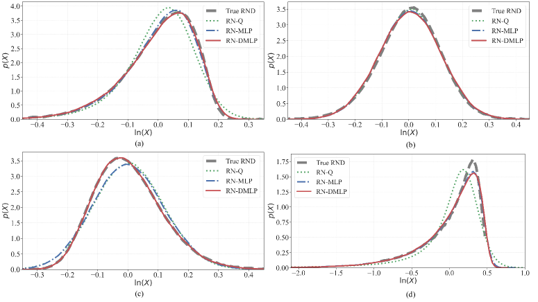
Figure 1 illustrates the true Heston RND alongside the recovered RNDs by the three models: RN-Q, RN-MLP, and RN-DMLP. Our models demonstrate a notable capability to capture the primary characteristics of the true RND, including main shapes and tail behaviors. Particularly, the RN-DMLP model stands out by exhibiting superior performance. It effectively approximates the true RND and even achieves perfect recovery of the left-skewed or right-skewed RND, surpassing the performance of the other two which show a slight degradation. These simulation outcomes provide robust evidence of the reliability of our proposed models in extracting the RND from option data.

4.3 Empirical Studies with S&P 500 Options

In this section, our aim is to compare the empirical performance of our three models with that of classical option pricing models using a real-world dataset. We utilize European option data of the S&P 500, obtained from the OptionMetrics IvyDB US database, accessed through the Wharton Research Data Services.

Data and Preprocessing.

We collect the daily European option prices of S&P 500 from OptionMetrics for the period spanning from January 4, 1996, to February 28, 2023. Initially, we filter out observations with bid or ask prices lower than $0.025 to mitigate the impact of decimalization, in line with the approach outlined in Song and Xiu, (2016). Additionally, we approximate the option price using the average of the bid and ask (the mid quote). Options with invalid implied volatility are excluded from the dataset. The daily closing price of the index serves as the underlying price in our studies. We normalize the time-to-maturity by dividing the days to maturity by 365. The risk-free interest rate $r$ is linearly interpolated to align with the option maturity.

Training, Testing, and Extreme-Moneyness Sets.

To compare our models against classical models, at each observation date, we split all options into three disjoint sets. Except for the training set, we evaluate the pricing performance on both a testing set and an extreme moneyness option set. To achieve this, we arrange strike prices $K$ in ascending order for a given option maturity and select options with moneyness $K/S_{t}$ falling within the range of $[0.8,1.2]$ as the training-testing set. We allocate odd-indexed options to the training set and even-indexed options to the testing set. Options outside this moneyness range are categorized as the extreme moneyness option set. The options in the testing set and extreme moneyness set are solely for prediction or out-of-sample evaluation purpose, while the training set is for calibration. The training is done via the MSE loss, i.e.,

$$L(C_{i},\hat{C}_{i})=(C_{i}-\hat{C}_{i})^{2},\quad\text{and }L(P_{j},\hat{P}_{j})=(P_{j}-\hat{P}_{j})^{2},$$

and the out-of-sample prediction/evaluation is conducted using both MSE and relative MSE, the latter of which is computed by

$$L(C_{i},\hat{C}_{i})=(\hat{C}_{i}/C_{i}-1)^{2},\quad\text{and }L(P_{j},\hat{P}_{j})=(\hat{P}_{j}/P_{j}-1)^{2}.$$

The training process involves sampling $Z=[Z_{1},Z_{2},\dots,Z_{N}]$ from $\mathbb{N}(0,1)$ with $N=1e^{6}$.

4.3.1 Two Experimental Settings and Results

It is important to note that options on the S&P 500 display a diverse range of time-to-maturities ($\tau$) on each trading day. Some traditional models, such as the double log-normal (Bahra,, 1997), generalized beta (Bookstaber et al.,, 1987), and Edgeworth expansion (Rubinstein et al.,, 1998) models, are generally calibrated for a single $\tau$ value. In contrast, our proposed models represent a significant advancement by allowing multiple $\tau$ values, hence allowing for the modeling of $\tau$-dependent RNDs, forming a term structure of RNDs. To be consistent with those previous models, we investigate two experimental settings: a single $\tau$ setting and a multiple $\tau$ setting.

Figure 2: Pricing performance under the single $\tau$ setting. The $\log_{10}\text{MSE}$ (averaged in every quarter) on the testing set is plotted against varying time for each model. The shaded areas represent the financial crisis periods. Overall, RN-DMLP achieves the best performance.

Table 1: Pricing performance averaged over all years under single $\tau$ setting. The smallest loss is highlighted in bold, and the second smallest is in italics. We present the results on both the testing set and the extreme-moneyness set, under the metrics of both MSE and relative MSE. Consistently, RN-DMLP achieves the best performance.

		RN-Q	RN-MLP	RN-DMLP	DLN	GB	EW
Testing	MSE	1032.43	122.57	26.03	67.73	1171.84	1058.79
	Relative	0.33	0.30	0.16	0.22	0.47	0.52
Extreme	MSE	1279.49	168.48	93.64	262.14	1452.08	$1.1e^{6}$
	Relative	1.39	0.69	0.53	2.58	3.22	$6.4e^{4}$

Single Time-to-maturity Setting.

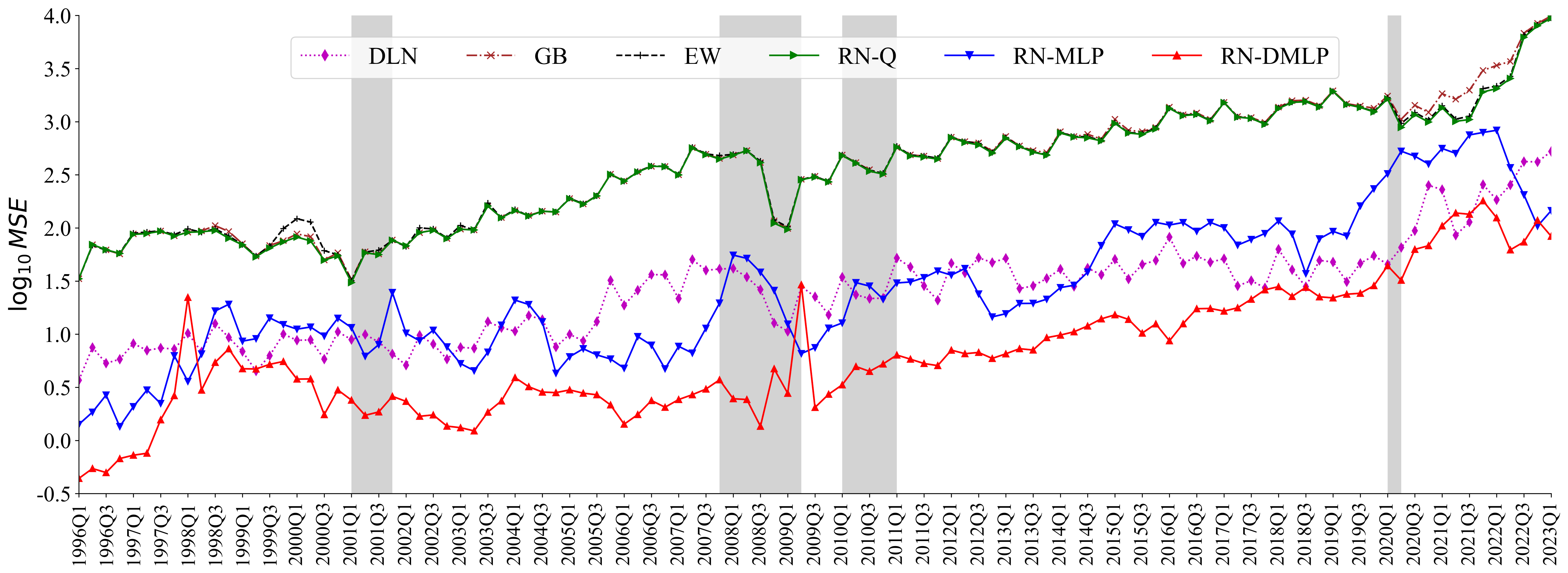
In our first experimental setting, the models are calibrated based on option contracts with each specific time-to-maturity ($\tau$) separately. Given the presence of different maturities on each trading day, this approach yields multiple calibrated models on a daily basis. This experimental setup is consistent with standard practices commonly employed in the literature. We benchmark our models, RN-Q, RN-MLP, and RN-DMLP, against three classical models: the double log-normal (DLN), the generalized beta (GB), and the Edgeworth expansion (EW). Our models are calibrated following the default configurations described in Section 4.1, while the benchmark models are calibrated using the R Package Risk-neutral Density Extraction (Hamidieh,, 2014). Subsequently, these calibrated models are utilized to predict option prices in both the testing set and the extreme-moneyness set. We present the mean squared error (MSE) and relative MSE to evaluate the out-of-sample pricing performance and extreme-moneyness pricing capabilities of these models.

The empirical evidence presented in Figure 2 clearly demonstrates the superior performance of our RN-DMLP model, as it consistently exhibits lower MSE levels compared to alternative models across years from 1996 to 2023. Specifically, the MSE of the RN-DMLP model remains below $10^{1}$ most of the time and does not exceed $10^{3}$, indicating a significant improvement over its competitors. Our RN-MLP model displays comparable accuracy to the DLN method. Table 1 further corroborates that our proposed RN-DMLP model consistently achieves lower MSE and relative MSE on both the testing set and the extreme-moneyness set compared to other baseline models. The DLN method shows acceptable performance on the testing set, but exhibits noticeably lower pricing accuracy when dealing with extreme-moneyness options. The EW method appears unstable, as it sometimes reaches the MSE of $10^{6}$. Overall, our RN-DMLP model demonstrates superior predictive accuracy on both sets compared to all other models.

Multiple Time-to-maturities Setting.

In the subsequent analysis, we delve into the multiple $\tau$ setting. This involves calibrating a single model using multiple option contracts with a range of time-to-maturities $\tau$ on a trading day. We continue to use the same setting to divide and obtain the training set, testing set, and extreme-moneyness set. To better guarantee the no-arbitrage Constraint 5 and 6, we establish a dense grid of time-to-maturity $\tau$ and strike price $K$, to be used in the penalty term in Eqn.(24). Suppose the options from the market on a trading day have $N_{\tau}$ maturities $\{\tau_{i}\}_{i=1}^{N_{\tau}}$ and $N_{K}$ strike prices $\{K_{i}\}_{i=1}^{N_{K}}$. The synthetic grid $\mathcal{I}^{syn}$ is given as follows:

$$\mathcal{I}^{syn}=\left\{(\tau^{syn},K^{syn}):\tau^{syn}\in\left\{\frac{\tau_{[i]}+\tau_{[i+1]}}{2}\right\}\cup\{\tau_{i}\},K^{syn}\in\left\{\frac{K_{[i]}+K_{[i+1]}}{2}\right\}\cup\{K_{i}\}\right\},$$ (26)

where $\tau_{[i]}$ or $K_{[i]}$ is the $i$-th element in ascending order in the set $\{\tau_{i}\}$ or $\{K_{i}\}$. We set about $1,000$ points in $\mathcal{I}^{syn}$ in total on each training day for training our models.

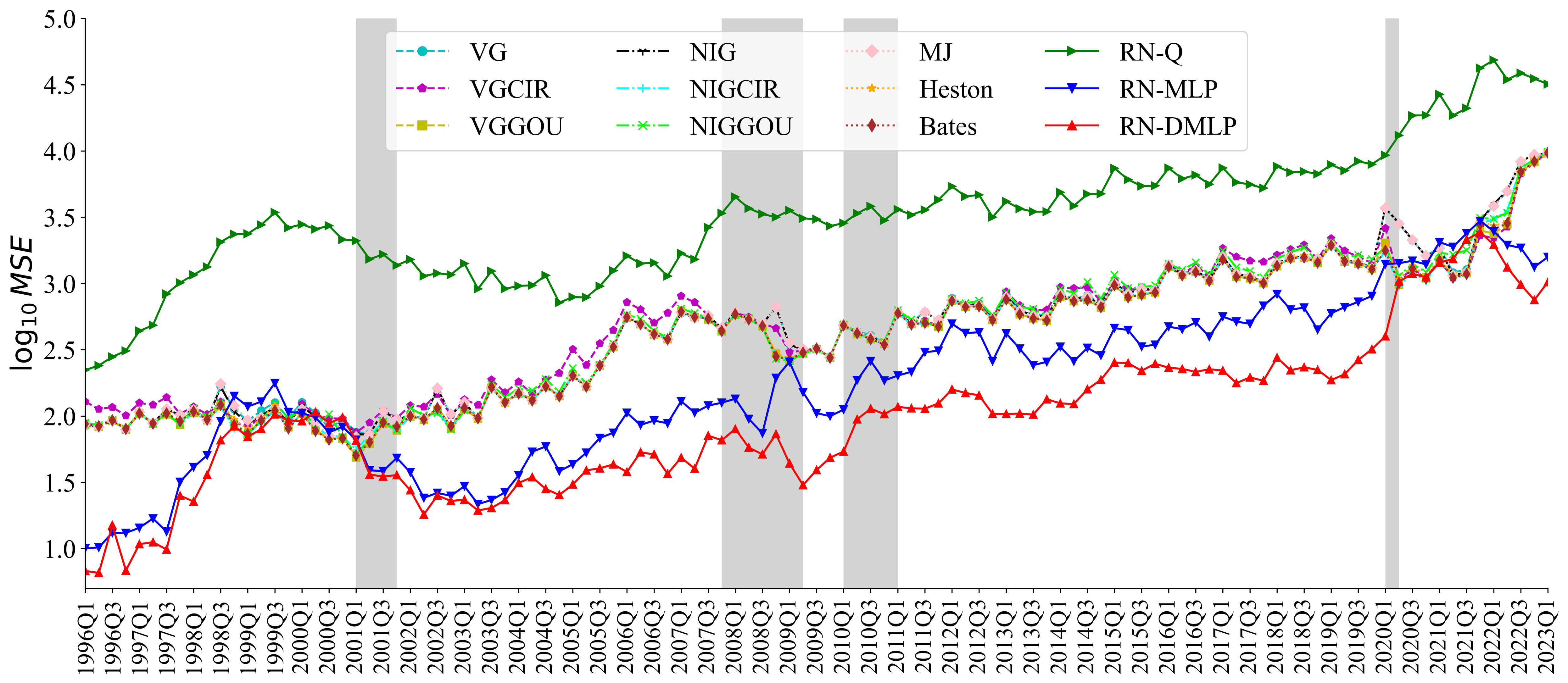
Subsequently, we calibrate our models with option data, incorporating multiple $\tau$ values as inputs. To provide a comprehensive and reliable evaluation of the models’ performance in this setting, we conduct extensive comparisons involving a total of 9 classical models and their variants: variance gamma (VG) (Madan and Seneta,, 1990), variance gamma with Cox–Ingersoll–Ross process (VGCIR) (Schoutens and Symens,, 2003), variance gamma with Gamma Ornstein–Uhlenbeck clock process (VGGOU) (Carr et al.,, 2003), normal inverse Gaussian (NIG) (Barndorff-Nielsen,, 1997), normal inverse Gaussian with Cox–Ingersoll–Ross process (NIGCIR) (Carr et al.,, 2003), normal inverse Gaussian with Gamma Ornstein–Uhlenbeck clock process (NIGGOU) (Eberlein and Raible,, 1999), Merton with jumps (MJ) (Merton,, 1976), Heston method (Heston,, 1993), and Bates method (Bates,, 1996). These models will be calibrated using MATLAB packages provided by (Kienitz and Wetterau,, 2013).

Figure 3: Pricing performance under the multiple $\tau$ setting. The $\log_{10}\text{MSE}$ (averaged in every quarter) on the testing set is plotted against varying time for each model. The shaded areas represent the financial crisis periods. Overall, RN-DMLP achieves the best performance and RN-MLP is the second best.

Table 2: Pricing performance averaged over all years under multiple $\tau$ setting. The smallest loss is highlighted in bold, and the second smallest is in italics. We present the results on both the testing set and the extreme-moneyness set, under the metrics of both MSE and relative MSE. Overall, RN-DMLP achieves the best performance and RN-MLP is the second best.

		RN-Q	RN-MLP	RN-DMLP	VG	VGCIR	VGGOU	NIG	NIGCIR	NIGGOU	MJ	Heston	Bates
Testing	MSE	8289.66	559.70	345.81	1288.87	1152.93	1085.58	1288.52	1132.56	1206.11	1282.02	1113.92	1092.38
	Relative	3748.19	1.86	0.39	2.63	5.55	1.01	2.10	3.83	12.48	1.64	4.83	2.71
Extreme	MSE	3094.16	584.43	383.47	1480.19	1393.48	1435.14	1501.03	1693.30	1454.30	1541.11	2325.52	1960.93
	Relative	1970.65	2.96	1.07	4.65	15.17	8.25	5.32	28.28	18.47	12.03	1887.84	1649.52

Figure 3 reveals that our models RN-MLP and RN-DMLP incorporating neural networks achieve a substantial reduction in MSE compared to the parametric method RN-Q. They also demonstrate evident superiority to the 9 classical methods, achieving MSE levels in the order of approximately $10^{2}$ most of the time. Table 2 further substantiates the superior performance of our RN-DMLP model, as it consistently obtains lower MSE and relative MSE on both the testing set and the extreme-moneyness set. Notably, RN-DMLP attains nearly an order of magnitude reduction in MSE compared to the classical competitors. Our RN-MLP model also exhibits lower MSE and relative MSE, especially when pricing the extreme-moneyness options when compared to the classical models. This table further indicates that the classical models exhibit similar performance levels. Both Figure 3 and Table 2 clearly showcase the significant superiority of our proposed models.

4.3.2 Testing the Stability of Extracted RND

In this section, we aim to conduct an experiment to assess the stability of the RND extracted by our proposed models and a total of 12 competitors previously mentioned. For this purpose, we randomly select S&P 500 option data on a specific trading day (August 15, 2019) with a specific time-to-maturity ($\tau=$ 400 days) to perform the experiment. To assess the RND stability, we introduce small perturbations to the observed option data. These small perturbations are equivalent to one tick size of the S&P 500 option prices, which is $0.25. Every option price in the training set will randomly obtain either an addition or a subtraction of one tick. We then re-estimate the RND using our models and the twelve competitors. This procedure is repeated 50 times, allowing us to measure the deviations in perturbed RNDs.

Given the subtle nature of these perturbations, the resultant changes in the RNDs should be negligible. Models that exhibit smaller shifts in distribution in response to these perturbations are considered to have superior stability. However, the direct comparison of a large number of probability density functions (PDFs) poses a significant analytical challenge. To address this, we focus our evaluation on the variations in the distributional characteristics, specifically on the standard deviations of ten PDF characteristics across the fifty trials of perturbations. These standard deviations serve as our indicators of RND stability. The ten PDF characteristics are: the mean $\mu$, the standard deviation $\sigma$, the skewness, Pearson median-based skewness defined as $\text{Skew}_{PM}=\frac{\mu-X_{50}}{\sigma}$ where $X_{50}$ is the 50%-quantile, the asymmetry measure defined as $\text{Skew}_{AM}=\frac{X_{75}-X_{50}}{X_{50}-X_{25}}$, the kurtosis, and four tail-side percentiles $X_{01},X_{05},X_{95},X_{99}$.

Table 3: The table presents the standard deviations of the RND characteristics across fifty trials of perturbations as estimated by various models. Lower values in the table indicate superior stability of the estimated RND. The first row, denoted as MSE, represents the average mean square pricing error across the fifty trials. It is unequivocal that the RN-DMLP model exhibits the highest level of stability.

	RN-Q	RN-MLP	RN-DMLP	DLN	GB	EW	VG	VGCIR	VGGOU	NIG	NIGCIR	NIGGOU	MJ	Heston	Bates
MSE	234.07	132.81	19.08	43.76	224.33	305.70	184.71	202.51	182.68	1337.08	214.76	231.69	173.85	185.30	177.54
$\mu$	0.01	0.01	0.01	350.95	117.28	19.68	0.01	1.87	0.57	23.19	1.33	2.77	0.05	0.64	0.48
$\sigma$	0.15	0.06	0.07	520.83	92.14	30.17	0.06	34.09	30.51	0.25	31.26	45.98	0.09	31.36	30.73
Skewness	7.53	0.18	0.55	0.21	0.13	0.06	$1.39e^{4}$	5.02	3.19	$3.73e^{4}$	56.53	4.64	$2.01e^{6}$	0.43	0.55
$\text{Skew}_{PM}$	0.04	0.05	0.10	0.14	0.11	0.10	6963.22	0.06	0.08	$2.10e^{4}$	0.10	0.08	$1.04e^{6}$	0.09	0.10
$\text{Skew}_{AM}$	0.06	0.09	0.13	0.23	0.23	0.23	0.00	0.11	0.16	0.54	0.17	0.15	0.06	0.16	0.20
Kurtosis	786.09	0.20	1.47	0.82	0.43	0.23	$1.14e^{9}$	395.93	319.15	$1.15e^{10}$	$2.57e^{4}$	124.18	$2.67e^{13}$	21.38	30.24
$X_{01}$	0.46	0.18	0.24	304.94	304.94	304.94	0.22	114.88	115.09	22.98	124.90	134.22	0.26	121.00	114.05
$X_{05}$	0.14	0.12	0.15	261.69	261.69	261.69	0.06	60.23	64.26	23.02	66.17	64.21	0.15	66.50	64.20
$X_{95}$	0.07	0.08	0.06	208.75	208.75	208.75	0.00	28.11	26.93	23.20	27.67	32.46	0.05	27.36	32.62
$X_{99}$	0.09	0.11	0.06	290.32	290.32	290.32	0.00	137.91	43.25	23.19	39.74	47.84	0.09	40.04	53.45

Figure 4: Original and the perturbed RNDs of the underlying price at the maturity date estimated by our model RN-DMLP, which is obtained directly from the estimated RNDs of the log-return.

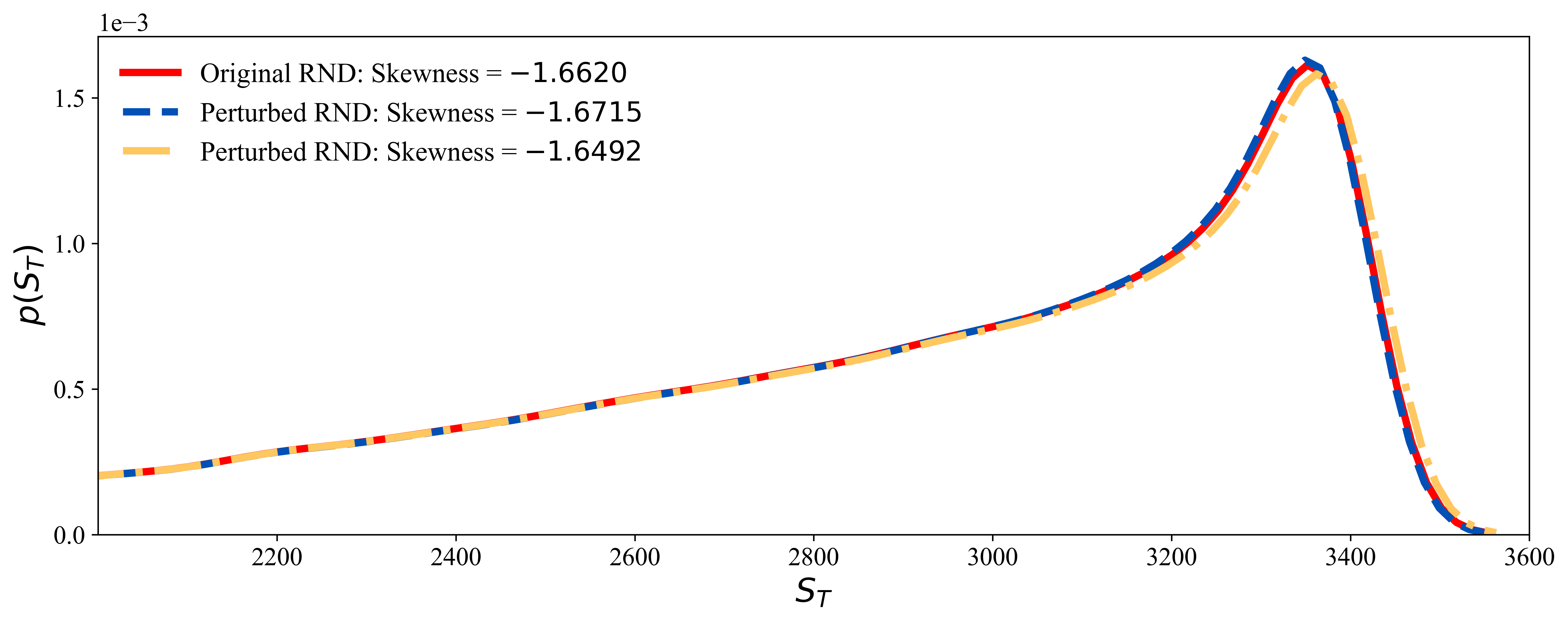
Table 3 presents the standard deviations of the RND characteristics obtained from fifty trials of perturbations given by various models. The table demonstrates that our three proposed models exhibit the most commendable stability in the extracted RND, as evidenced by consistently lower standard deviations across all ten RND characteristics. Moreover, our models RN-MLP and RN-DMLP display comparable stability in extracting RND, with identical levels of standard deviations. Both models marginally outperform RN-Q, which exhibits a larger deviation in its RND kurtosis. Among the other twelve competitors, it is notable that the three models based on distributional assumptions (DLN, GB, and EW) show greater stability in higher-order moments (skewness and kurtosis) but exhibit more variability in the first and second-order moments (mean and variance), compared to the remaining nine methods. The nine methods that incorporate stochastic processes remain relatively stable in most RND characteristics, albeit occasionally exhibiting extreme values up to $10^{4}$ or even larger.

In the first row of Table 3, we present the average MSE across the fifty trials of perturbations. Our proposed model, RN-DMLP, not only achieves the most accurate predictions but also ensures the highest stability, as evidenced by the lowest MSE and minimal changes in the extracted RNDs. These results underscore the robustness and reliability of our proposed models. Figure 4 illustrates the original RND extracted by RN-DMLP, alongside the RNDs with minimum and maximum skewness among these fifty trials of perturbations. It is important to emphasize that the RNDs depicted in Figure 4 represent the distributions of the underlying asset price at maturity, which are derived directly from the estimated RNDs of the log-return. We observe that the distributions are nearly indistinguishable, with the two perturbed RNDs being highly consistent with the original one, further validating the stability of our method.

5 Higher-Order Moments of Extracted RNDs

Table 4: The ratio of left and right skewed RNDs extracted by the model RN-DMLP.

	Left-skewed	Right-skewed	Total
Number of RNDs	64383 (98.72%)	833 (1.28%)	65216

Figure 5: This figure displays the monthly risk-neutral volatility (RNM2) extracted by the RN-DMLP model and the VIX index from January 1996 to February 2023, as well as their correlation coefficient. The RNM2 is computed from the RND extracted using option contracts with time-to-maturities between 25 and 35 days. The shaded grey areas represent the financial crisis periods. In the figure, both series have been standardized to have zero mean and unit variance.

Figure 6: Risk-neutral moments’ summary statistics and the representative RNDs with different time-to-maturities between 1 week (1W) and 1 year (1Y). Subfigure (a) presents the box plots of the three risk-neutral moments RNM2 – RNM4 in every time-to-maturity group. We observe increasing patterns in the second and fourth-order moments, and a decreasing pattern in the third moment as the time-to-maturity increases. Subfigure (b) exhibits two representative RNDs within each time-to-maturity group, with each column corresponding to a group. In the first row of plots, the RNDs have a skewness level of 25th-percentile in their respective groups. In the second row, the RNDs have a skewness level of 75th-percentile.

(a) Risk-Neutral Volatility

(b) Risk-Neutral Volatility

(c) Risk-Neutral Skewness

(d) Risk-Neutral Skewness

(e) Risk-Neutral Kurtosis

(f) Risk-Neutral Kurtosis

Figure 7: The term structures of risk-neutral moments (RNM2 – RNM4) produced by our RN-DMLP model (a, c, and e) and by the Heston model (b, d, and f), with the time horizon increasing from 1 week to 1 year. We select five trading days for RN-DMLP and three parameter settings for the Heston. The term structures of RNM3 and RNM4 produced by RN-DMLP demonstrate more flexible patterns, such as the strictly monotonic RNM3/RNM4, the nearly constant RNM3/RNM4, and the slightly decreasing RNM4 when the time-to-maturity exceeds three months. In contrast, the Heston model generates strictly monotonic term structures only, indicating a relatively restrictive range of asset dynamics it can model. For RNM2, both models yield strictly increasing term structures, which is consistent with our expectations. We attribute the success of RN-DMLP to its ability to offer flexible term structures for skewness (RNM3) and kurtosis (RNM4).

In this section, our aim is to derive valuable insights about the RNDs of S&P 500 returns extracted by the RN-DMLP model (not S&P 500 prices). As detailed in Section 4.3.1 and 4.3.2, we conducted empirical experiments to rigorously evaluate the option pricing performance. To commence our investigation here, we collect the extracted RNDs from the well-calibrated RN-DMLP models. The RND in Eqn.(20) is in a generative machine learning form, allowing us to easily compute the risk-neutral moments as well as density values through sampling. We examine the risk-neutral moments and density graphs of RNDs to show what implications they have. Furthermore, we conduct a comparative analysis with the monthly VIX index, which is a well-established and widely utilized risk measure based on S&P 500. The sample period we consider spans from January 1996 to February 2023. In the following, we present four key findings.

Firstly, throughout the entire sample period from January 1996 to February 2023, there are 65,216 RNDs in total. Table 4 reports that around 98.72% of cases are left-skewed while around 1.28% of cases are right-skewed. It indicates the dominance of left-skewed RNDs in the market. Secondly, we display the monthly risk-neutral volatility series and the time series of VIX index in Figure 5. The risk-neutral volatility is computed from the RND extracted using option contracts with time-to-maturities between 25 and 35 days. As shown in the figure, the two series coincide with each other and the correlation coefficient is 0.9120. These two findings not only align with intuitions on the financial markets, but also verify the rationality and robustness of the extracted RNDs from our model.

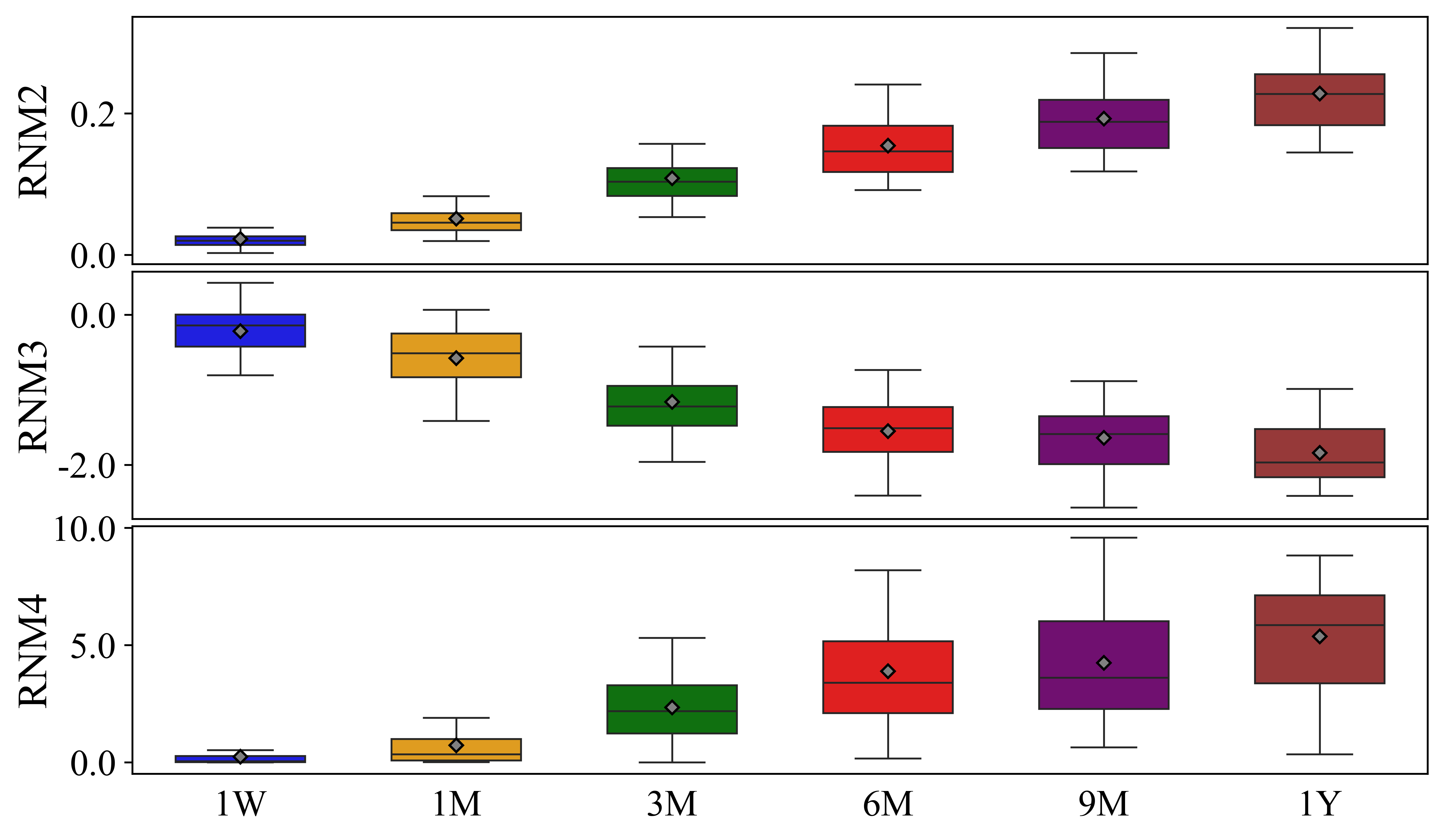
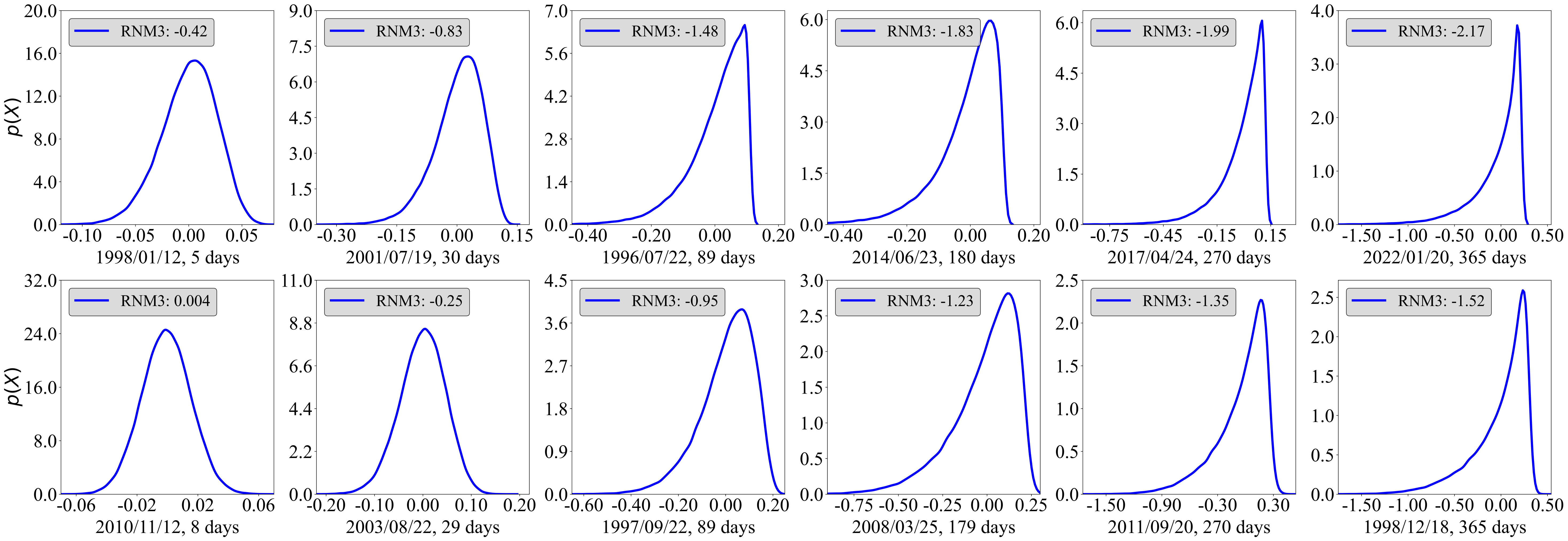
Thirdly, based on various time-to-maturities (one week, one month, three months, six months, nine months, and one year), we summarize the statistics of the risk-neutral moments and illustrate some extracted RNDs in Figure 6. Subfigure (a) presents six box plots of the three risk-neutral moments RNM2 – RNM4, with the time-to-maturity increasing from 1 week (1W) to 1 year (1Y). We observe increasing patterns in the second and fourth-order moments, and a decreasing pattern in the third moment as the time-to-maturity increases. Subfigure (b) exhibits two representative RNDs within each time-to-maturity group, with each column corresponding to a group. In the first row of plots, the RNDs have a skewness level of 25th-percentile in their respective time-to-maturity groups. In the second row, the RNDs have a skewness level of 75th-percentile.

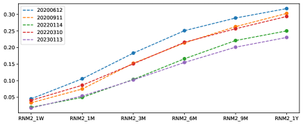
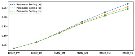
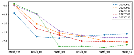
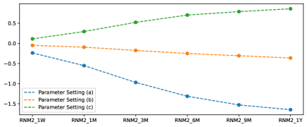
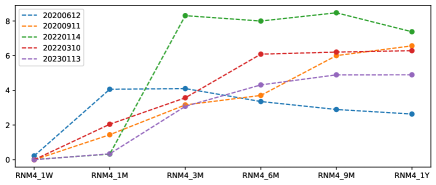
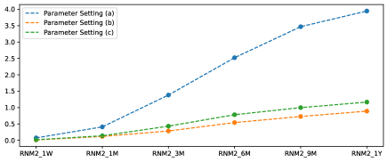
Finally, we investigate the term structures of the risk-neutral moments (RNMs) generated by the RN-DMLP model on each trading day and compare them with those generated by the Heston model. Figure 7 illustrates the term structures on five selected trading days, as well as those generated by three Heston models with parameters set as in Figure 1. The term structures of RNM3 and RNM4 produced by our RN-DMLP model demonstrate more flexible patterns, such as the strictly monotonic RNM3/RNM4, the nearly constant RNM3/RNM4, and the slightly decreasing RNM4 when the time-to-maturity exceeds three months. In contrast, the Heston model generates strictly monotonic term structures only, indicating a relatively restrictive range of asset dynamics it can model. For RNM2, both models yield strictly increasing term structures, which is consistent with our expectations. We attribute the success of the RN-DMLP model to its ability to offer flexible term structures for skewness (RNM3) and kurtosis (RNM4).

6 Conclusion

Extracting the risk-neutral density (RND) is a critical and challenging task in finance. In this paper, we introduce the risk-neutral generative network (RNGN) framework, featuring three generative models that do not rely on assumptions regarding the underlying asset price dynamics or the distributional families to which the RND belongs. Our proposed models adhere to the no-arbitrage constraints. In simulation studies, we generate option price data encompassing a range of RNDs with various shapes (including left-skewed, nearly normal, and right-skewed) to demonstrate that our three models can efficiently extract the true RND. In the empirical analysis, we compare the results obtained under our proposed framework with those derived from classical methodologies, utilizing option data of S&P 500. Empirical results underscore the superiority of our models in terms of pricing accuracy on both testing sets and extreme-moneyness sets. Our models further exhibit greater stability of the estimated RND. It is noteworthy that the RN-DMLP model performs exceptionally well, achieving an extremely low MSE level.

Our model RN-MLP incorporates a neural network known as Multilayer Perceptron (MLP), based on the structure of our initial model RN-Q. Our derived pricing formulas are based on Monte Carlo simulation, and rational considerations are taken into account when learning our network. We attribute the exceptional performance of RN-MLP to the learning capability of the neural network, which enables it to capture complex patterns in the data. Inspired by the idea of double log-normal density, we further combine two RN-MLPs to propose our third model, RN-DMLP, which exhibits remarkable performance with sufficiently low MSE levels on S&P 500 option data. We attribute the success of RN-DMLP to the increased flexibility of the distribution it can model. At last, we examine the risk-neutral moments and density graphs of RNDs, showing empirical findings that not only align with intuitions on the financial markets but also verify the rationality of the extracted RNDs. At last, through some analysis, we attribute the success of RN-DMLP to its ability to offer flexible term structures for risk-neutral skewness and kurtosis.

Appendix

A.1 Proof of Proposition 1

Proof.

We require $\frac{\partial\hat{C}_{M}}{\partial\tau}\geq 0$ and $\frac{\partial\hat{P}_{M}}{\partial\tau}\geq 0$. The former is equivalent to

$$\frac{\partial\hat{C}_{M}}{\partial\tau} =\frac{\partial}{\partial\tau}\left\{S_{t}e^{-r\tau}\frac{1}{N}\sum_{n=1}^{N}\left(e^{X(Z_{n},\tau;\theta^{M})}-S_{t}^{-1}K^{C}\right)^{+}\right\}$$

$$=-rS_{t}e^{-r\tau}\frac{1}{N}\sum_{n=1}^{N}\left(e^{X(Z_{n},\tau;\theta^{M})}-S_{t}^{-1}K^{C}\right)^{+}+S_{t}e^{-r\tau}\frac{1}{N}\sum_{n=1}^{N}\frac{\partial}{\partial\tau}\left(e^{X(Z_{n},\tau;\theta^{M})}-S_{t}^{-1}K^{C}\right)^{+}$$

$$=S_{t}e^{-r\tau}\frac{1}{N}\sum_{n=1}^{N}\frac{\partial}{\partial\tau}\left(e^{X(Z_{n},\tau;\theta^{M})}-S_{t}^{-1}K^{C}\right)\mathbb{I}_{\{e^{X(Z_{n},\tau;\theta^{M})}\geq S_{t}^{-1}K^{C}\}}$$

$$\quad-rS_{t}e^{-r\tau}\frac{1}{N}\sum_{n=1}^{N}\left(e^{X(Z_{n},\tau;\theta^{M})}-S_{t}^{-1}K^{C}\right)\mathbb{I}_{\{e^{X(Z_{n},\tau;\theta^{M})}\geq S_{t}^{-1}K^{C}\}}$$

$$=S_{t}e^{-r\tau}\frac{1}{N}\sum_{n=1}^{N}\left[\left(\frac{\partial X(Z_{n},\tau;\theta^{M})}{\partial\tau}-r\right)e^{X(Z_{n},\tau;\theta^{M})}+rS_{t}^{-1}K^{C}\right]\mathbb{I}_{\{e^{X(Z_{n},\tau;\theta^{M})}\geq S_{t}^{-1}K^{C}\}}$$

$$=S_{t}e^{-r\tau}\tilde{J}^{\tau}_{C}(\tau,K^{C},\theta^{M})\geq 0.$$

Similarly, we have

$$\frac{\partial\hat{P}_{M}}{\partial\tau} =\frac{\partial}{\partial\tau}\left\{S_{t}e^{-r\tau}\frac{1}{N}\sum_{n=1}^{N}\left(S_{t}^{-1}K^{P}-e^{X(Z_{n},\tau;\theta^{M})}\right)^{+}\right\}$$

$$=-rS_{t}e^{-r\tau}\frac{1}{N}\sum_{n=1}^{N}\left(S_{t}^{-1}K^{P}-e^{X(Z_{n},\tau;\theta^{M})}\right)^{+}+S_{t}e^{-r\tau}\frac{1}{N}\sum_{n=1}^{N}\frac{\partial}{\partial\tau}\left(S_{t}^{-1}K^{P}-e^{X(Z_{n},\tau;\theta^{M})}\right)^{+}$$

$$=S_{t}e^{-r\tau}\frac{1}{N}\sum_{n=1}^{N}\frac{\partial}{\partial\tau}\left(S_{t}^{-1}K^{P}-e^{X(Z_{n},\tau;\theta^{M})}\right)\mathbb{I}_{\{e^{X(Z_{n},\tau;\theta^{M})}\leq S_{t}^{-1}K^{P}\}}$$

$$\quad-rS_{t}e^{-r\tau}\frac{1}{N}\sum_{n=1}^{N}\left(S_{t}^{-1}K^{P}-e^{X(Z_{n},\tau;\theta^{M})}\right)\mathbb{I}_{\{e^{X(Z_{n},\tau;\theta^{M})}\leq S_{t}^{-1}K^{P}\}}$$

$$=S_{t}e^{-r\tau}\frac{1}{N}\sum_{n=1}^{N}\left[\left(r-\frac{\partial X(Z_{n},\tau;\theta^{M})}{\partial\tau}\right)e^{X(Z_{n},\tau;\theta^{M})}-rS_{t}^{-1}K^{P}\right]\mathbb{I}_{\{e^{X(Z_{n},\tau;\theta^{M})}\leq S_{t}^{-1}K^{P}\}}$$

$$=S_{t}e^{-r\tau}\tilde{J}^{\tau}_{P}(\tau,K^{P},\theta^{M})\geq 0.$$

In addition, the Constraint 6, upon substituting the expecation by the sample average and $\mu(\tau)$ by $r\tau G^{\mu}(\tau;\theta^{\mu})$ in Eqn.(8),

$$r\tau G^{\mu}(\tau;\theta^{\mu})+\ln\left(\frac{1}{N}\sum_{n=1}^{N}e^{\sigma\sqrt{\tau}\cdot Z_{n}\cdot[G^{Z}(Z_{n};\theta^{Z})+G^{\tau}(\tau;\theta^{\tau})+1]}\right)-r\tau=0,\quad\forall\tau>0,$$ (A.1)

is equivalent to setting $J^{\mu}_{M}(\tau,\theta^{M})=0$ where,

$$J^{\mu}_{M}(\tau,\theta^{M})=\left|r\tau\left(G^{\mu}(\tau;\theta^{\mu})-1\right)+\ln\left(\frac{1}{N}\sum_{n=1}^{N}e^{\sigma\sqrt{\tau}\cdot Z_{n}\cdot[G^{Z}(Z_{n};\theta^{Z})+G^{\tau}(\tau;\theta^{\tau})+1]}\right)\right|^{2}.$$ (A.2)

∎

References

- Ackerer et al., (2020) Ackerer, D., Tagasovska, N., and Vatter, T. (2020). Deep smoothing of the implied volatility surface. Advances in Neural Information Processing Systems, 33:11552–11563.
- Amilon, (2003) Amilon, H. (2003). A neural network versus black–scholes: a comparison of pricing and hedging performances. Journal of Forecasting, 22(4):317–335.
- Bahra, (1997) Bahra, B. (1997). Implied risk-neutral probability density functions from option prices: theory and application. Technical report, Bank of England.
- Baldi and Hornik, (1989) Baldi, P. and Hornik, K. (1989). Neural networks and principal component analysis: Learning from examples without local minima. Neural Networks, 2(1):53–58.
- Barndorff-Nielsen, (1997) Barndorff-Nielsen, O. E. (1997). Normal inverse gaussian distributions and stochastic volatility modelling. Scandinavian Journal of Statistics, 24(1):1–13.
- Bates, (1996) Bates, D. S. (1996). Jumps and stochastic volatility: Exchange rate processes implicit in deutsche mark options. The Review of Financial Studies, 9(1):69–107.
- Bookstaber et al., (1987) Bookstaber, R. M., McDonald, J. B., et al. (1987). A general distribution for describing security price returns. The Journal of Business, 60(3):401–424.
- Carr et al., (2003) Carr, P., Geman, H., Madan, D. B., and Yor, M. (2003). Stochastic volatility for lévy processes. Mathematical Finance, 13(3):345–382.
- Casella and Berger, (2024) Casella, G. and Berger, R. (2024). Statistical inference. CRC Press.
- Cont, (1997) Cont, R. (1997). Beyond implied volatility: Extracting information from options prices. Econophysics. Dordrecht: Kluwer.
- Cont, (2001) Cont, R. (2001). Empirical properties of asset returns: stylized facts and statistical issues. Quantitative Finance, 1(2):223.
- Cont and Vuletić, (2023) Cont, R. and Vuletić, M. (2023). Simulation of arbitrage-free implied volatility surfaces. Applied Mathematical Finance, 30(2):94–121.
- Cox and Ross, (1976) Cox, J. C. and Ross, S. A. (1976). The valuation of options for alternative stochastic processes. Journal of Financial Economics, 3(1-2):145–166.
- Davis and Hobson, (2007) Davis, M. H. and Hobson, D. G. (2007). The range of traded option prices. Mathematical Finance, 17(1):1–14.
- Dugas et al., (2000) Dugas, C., Bengio, Y., Bélisle, F., Nadeau, C., and Garcia, R. (2000). Incorporating second-order functional knowledge for better option pricing. Advances in Neural Information Processing Systems, 13.
- Eberlein and Raible, (1999) Eberlein, E. and Raible, S. (1999). Term structure models driven by general lévy processes. Mathematical Finance, 9(1):31–53.
- Fengler, (2009) Fengler, M. R. (2009). Arbitrage-free smoothing of the implied volatility surface. Quantitative Finance, 9(4):417–428.
- Föllmer and Schied, (2011) Föllmer, H. and Schied, A. (2011). Stochastic finance: an introduction in discrete time. Walter de Gruyter.
- Garcia and Gençay, (2000) Garcia, R. and Gençay, R. (2000). Pricing and hedging derivative securities with neural networks and a homogeneity hint. Journal of Econometrics, 94(1-2):93–115.
- Goodfellow et al., (2014) Goodfellow, I., Pouget-Abadie, J., Mirza, M., Xu, B., Warde-Farley, D., Ozair, S., Courville, A., and Bengio, Y. (2014). Generative adversarial nets. Advances in Neural Information Processing Systems, 27.
- Hamidieh, (2014) Hamidieh, K. (2014). Rnd: Risk neutral density extraction package. R package version, 1.
- Harrison and Kreps, (1979) Harrison, J. M. and Kreps, D. M. (1979). Martingales and arbitrage in multiperiod securities markets. Journal of Economic Theory, 20(3):381–408.
- Harrison and Pliska, (1981) Harrison, J. M. and Pliska, S. R. (1981). Martingales and stochastic integrals in the theory of continuous trading. Stochastic Processes and Their Applications, 11(3):215–260.
- Heston, (1993) Heston, S. L. (1993). A closed-form solution for options with stochastic volatility with applications to bond and currency options. The Review of Financial Studies, 6(2):327–343.
- Hornik et al., (1989) Hornik, K., Stinchcombe, M., and White, H. (1989). Multilayer feedforward networks are universal approximators. Neural Networks, 2(5):359–366.
- Hutchinson et al., (1994) Hutchinson, J. M., Lo, A. W., and Poggio, T. (1994). A nonparametric approach to pricing and hedging derivative securities via learning networks. The Journal of Finance, 49(3):851–889.
- Kienitz and Wetterau, (2013) Kienitz, J. and Wetterau, D. (2013). Financial modelling: Theory, implementation and practice with MATLAB source. John Wiley & Sons.
- Madan and Seneta, (1990) Madan, D. and Seneta, E. (1990). The variance gamma (vg) model for share market returns. Journal of Business, 63(4):511–524.
- Merton, (1976) Merton, R. C. (1976). Option pricing when underlying stock returns are discontinuous. Journal of Financial Economics, 3(1-2):125–144.
- Orosi, (2015) Orosi, G. (2015). Estimating option-implied risk-neutral densities: a novel parametric approach. Journal of Derivatives, 23(1):41.
- Roper, (2010) Roper, M. (2010). Arbitrage free implied volatility surfaces. preprint.
- Rubinstein et al., (1998) Rubinstein, M. et al. (1998). Edgeworth binomial trees. Journal of Derivatives, 5:20–27.
- Schmitt and Westerhoff, (2017) Schmitt, N. and Westerhoff, F. (2017). On the bimodality of the distribution of the s&p 500’s distortion: Empirical evidence and theoretical explanations. Journal of Economic Dynamics and Control, 80:34–53.
- Schoutens and Symens, (2003) Schoutens, W. and Symens, S. (2003). The pricing of exotic options by monte–carlo simulations in a lévy market with stochastic volatility. International Journal of Theoretical and Applied Finance, 6(08):839–864.
- Schweizer and Wissel, (2008) Schweizer, M. and Wissel, J. (2008). Arbitrage-free market models for option prices: The multi-strike case. Finance and Stochastics, 12:469–505.
- Song and Xiu, (2016) Song, Z. and Xiu, D. (2016). A tale of two option markets: Pricing kernels and volatility risk. Journal of Econometrics, 190(1):176–196.
- Wu and Yan, (2019) Wu, Q. and Yan, X. (2019). Capturing deep tail risk via sequential learning of quantile dynamics. Journal of Economic Dynamics and Control, 109:103771.
- Yan et al., (2019) Yan, X., Wu, Q., and Zhang, W. (2019). Cross-sectional learning of extremal dependence among financial assets. Advances in Neural Information Processing Systems, 32.
- Yan et al., (2018) Yan, X., Zhang, W., Ma, L., Liu, W., and Wu, Q. (2018). Parsimonious quantile regression of financial asset tail dynamics via sequential learning. Advances in Neural Information Processing Systems, 31.
- Yang et al., (2017) Yang, Y., Zheng, Y., and Hospedales, T. (2017). Gated neural networks for option pricing: Rationality by design. In Proceedings of the AAAI Conference on Artificial Intelligence, volume 31.