Factor Augmented Matrix Regression

Abstract

We introduce Factor-Augmented Matrix Regression (FAMAR) to address the growing applications of matrix-variate data and their associated challenges, particularly with high-dimensionality and covariate correlations. FAMAR encompasses two key algorithms. The first is a novel non-iterative approach that efficiently estimates the factors and loadings of the matrix factor model, utilizing techniques of pre-training, diverse projection, and block-wise averaging. The second algorithm offers an accelerated solution for penalized matrix factor regression. Both algorithms are supported by established statistical and numerical convergence properties. Empirical evaluations, conducted on synthetic and real economics datasets, demonstrate FAMAR’s superiority in terms of accuracy, interpretability, and computational speed. Our application to economic data showcases how matrix factors can be incorporated to predict the GDPs of the countries of interest, and the influence of these factors on the GDPs.

Keywords: Matrix factor models; Matrix regression; Factor-augmented regression; Diversified projections; High-dimensionality.

1 Introduction

Matrix-variate data are commonly encountered in diverse domains nowadays, such as finance, economics, spatio-temporal data, healthcare, images, and social networks (Chen et al., 2020, 2023). In many problems, especially in high-dimensional regimes, it is common that matrix covariates assume low-rank structure or can be well approximated by low-rank matrices as exemplified by factor models (Wainwright, 2019; Chen & Fan, 2021). The outcomes of interest are directly influenced by latent low-rank matrix factors, not by the observable matrix covariates themselves. For instance, autism diagnosis relies on identifying specific patterns within brain connectivity networks, underscoring a direct link to reduced-dimensionality factors (Nogay & Adeli, 2020); regional GDP is shaped by the condensed economic indicators found within spatial-temporal housing data (Kopoin et al., 2013); and the GDP growth of countries is determined by underlying economic factors, demonstrating a direct relationship with these distilled elements (Banerjee et al., 2005).

To incorporate the matrix factor structure in matrix regressions, we introduce the Factor Augmented Matrix Regression (FAMAR) for observed random variables $\left\{\left(y_{i},\boldsymbol{X}_{i}\right),\;i\in[n]\right\}$, in which $y_{i}$ is a scalar response of interest and $\boldsymbol{X}_{i}$ is a $p_{1}\times p_{2}$ covariate matrix, defined as

$$\begin{cases}&y_{i}=\left\langle\boldsymbol{A}^{*},\boldsymbol{F}_{i}\right\rangle+\left\langle\boldsymbol{B}^{*},\boldsymbol{U}_{i}\right\rangle+\varepsilon_{i},\qquad\text{\it Matrix Factor Regression (MFR)}\\ &\boldsymbol{X}_{i}=\boldsymbol{R}^{*}\boldsymbol{F}_{i}\boldsymbol{C}^{*\top}+\boldsymbol{U}_{i},\qquad\qquad\hskip 14.63881pt\text{\it Matrix Factor Model (MFM)}\end{cases}$$ (1)

where $\boldsymbol{F}_{i}$ is the ${k_{1}\times k_{2}}$ latent factor matrix of lower dimensions $k_{j}\ll p_{j}$ for $j=1,2$, $\boldsymbol{U}_{i}$ is the unobserved idiosyncratic matrix, and $\boldsymbol{R}^{*}$ of dimension $p_{1}\times k_{1}$ and $\boldsymbol{C}^{*}$ of dimension $p_{2}\times k_{2}$ are the loading matrices of the Matrix Factor Model (MFM) (Chen & Fan, 2021). The impact of covariate matrix $\boldsymbol{X}_{i}$ on outcome $y_{i}$ is through the latent factors $\boldsymbol{F}_{i}$ and unobserved idiosyncratic matrix $\boldsymbol{U}_{i}$ with matrices $\boldsymbol{A}^{*}$ of dimension $k_{1}\times k_{2}$ and $\boldsymbol{B}^{*}$ of dimension $p_{1}\times p_{2}$ as the regression coefficient matrices of the Matrix Factor Regression (MFR). As the first component in MFR is the low-dimensional factor effect, the coefficient $\boldsymbol{A}^{*}$ can be estimated without any structures. We consider both sparse and low-rank structure for the regression coefficient matrix $\boldsymbol{B}^{*}$ since it is high-dimensional.

As practitioners harness the power of various data, model (1) has wide applications in economics and finance. For example, $y_{i}$ represents the monthly GDP of a country of interest, and $\boldsymbol{X}_{i}\in\mathbb{R}^{p_{1}\times p_{2}}$ consists of the $p_{2}$ economic variables collected from $p_{1}$ different countries. Model (1) is able to separate economic common factor $\boldsymbol{F}_{i}$ and idiosyncratic shocks $\boldsymbol{U}_{i}$ and provide economists with their respective impacts on the GDP of one country of interest. A salient feature of model (1) is that the association between the response $y_{i}$ and the covariate matrix $\boldsymbol{X}_{i}$ is established directly through the factor $\boldsymbol{F}_{i}$ and idiosyncratic matrix $\boldsymbol{U}_{i}$. This structure makes covariate inputs much weakly correlated and relates to various traditional models, as illustrated below.

Example 1 (Matrix regression with MFM covariates).

Matrix regression is written as

$$\begin{cases}&y_{i}=\left\langle\boldsymbol{B}^{*},\boldsymbol{X}_{i}\right\rangle+\varepsilon_{i},\hskip 25.83325pt\text{\it Matrix Regression (MR)}\\ &\boldsymbol{X}_{i}=\boldsymbol{R}^{*}\boldsymbol{F}_{i}\boldsymbol{C}^{*\top}+\boldsymbol{U}_{i},\hskip 12.91663pt\text{\it Matrix Factor Model (MFM)}\end{cases}$$ (2)

Model (2) is a special case of model (1) with $\boldsymbol{A}^{*}={\boldsymbol{R}^{*}}^{\top}\boldsymbol{B}^{*}\boldsymbol{C}^{*}$.

While we directly observe $\boldsymbol{X}_{i}$, using the matrix regression model (2) might seem straightforward. The influence of the latent factor $\boldsymbol{F}_{i}$ in model (2) is represented as ${\boldsymbol{R}^{*}}^{\top}\boldsymbol{B}^{*}\boldsymbol{C}^{*}$. However, the general FAMAR model introduces $\boldsymbol{\Phi}^{*}:=\boldsymbol{A}^{*}-\boldsymbol{R}^{\top}\boldsymbol{B}^{*}\boldsymbol{C}$, which quantifies the additional impact of the latent factor $\boldsymbol{F}_{i}$ in model (1) that is not accounted for by the observed predictor $\boldsymbol{X}_{i}$ in model (2).

Example 2 (Reduce-rank matrix regression).

Low-rank matrix regression $y_{i}=\left\langle\boldsymbol{B}^{*},\boldsymbol{X}_{i}\right\rangle+\varepsilon_{i}$ corresponds to a special case of (1) with low-rank coefficient matrix $\boldsymbol{B}^{*}$, matrix factor $\boldsymbol{F}_{i}=0$ and $\boldsymbol{U}_{i}=\boldsymbol{X}_{i}$ when $\boldsymbol{X}_{i}$ does not admit a factor structure, and $\boldsymbol{\Phi}^{*}=0$ when it does.

Example 3 (Sparse matrix regression).

Sparse matrix regression $y_{i}=\left\langle\boldsymbol{B}^{*},\boldsymbol{X}_{i}\right\rangle+\varepsilon_{i}$ is a special case of model (1) with sparse coefficient matrix $\boldsymbol{B}^{*}$, and $\boldsymbol{X}_{i}$ has not low-rank component, i.e., $\boldsymbol{F}_{i}=0$ and $\boldsymbol{U}_{i}=\boldsymbol{X}_{i}$.

There are several advantages of considering the more general model (1). First, in reality, especially when the columns and rows of $\boldsymbol{X}_{i}$ are highly correlated, the leading factors are likely to make additional contributions to the outcome, beyond a fixed portion represented by $\boldsymbol{A}^{*}={\boldsymbol{R}^{*}}^{\top}\boldsymbol{B}^{*}\boldsymbol{C}^{*}$ in model (2). To this end, model (1) involves incorporating the primary factors into a low-rank regression that extends the linear space defined by $\boldsymbol{X}_{i}$ in useful ways by noting that using $\boldsymbol{F}_{i}$ and $\boldsymbol{U}_{i}$ as covariates are the same as the usage of $\boldsymbol{F}_{i}$ and $\boldsymbol{X}_{i}$. In addition, even when model (2) is correctly specified, model (1) is helpful in dealing with the colinearity of $\boldsymbol{X}_{i}$ due to the factor structure (Fan, Ke & Wang, 2020). This is also confirmed in our empirical analysis. When covariates $\boldsymbol{X}_{i}$ are highly correlated, direct low-rank regression on $\boldsymbol{X}_{i}$’s often overestimates the rank due to their dependency structure, reducing the effectiveness of regularization and the interpretability of estimation. FAMAR enhances performance by utilizing the space spanned by $(\boldsymbol{F}_{i},\boldsymbol{U}_{i})$, which is the same as that span by $(\boldsymbol{F}_{i},\boldsymbol{X}_{i})$, with augmented feature $\boldsymbol{F}_{i}$, capitalizing further on underlying information. Additionally, its factor model approach decorrelates the covariance matrix, leading to coefficient estimators that are both more interpretable and stable.

Factor augmentations in the vector contexts have been studied under various settings and shown to be powerful (Fan, Ke & Wang, 2020; Zhou et al., 2021; Fan & Gu, 2022; Fan et al., 2023). In contrast, little work has been done on the matrix-variate problems. Matrix-variate settings are intrinsically different because of their multidimensional structure, where low rankness comes into play. Linear and generalized matrix regression have been studied in Zhou & Li (2014); Wang et al. (2017); Fan et al. (2019). However, model (1) in the present paper is different in that the association between $y_{i}$ and $\boldsymbol{X}_{i}$ is not direct as those in the literature but rather through the latent variables $\boldsymbol{F}_{i}$ and $\boldsymbol{U}_{i}$. We present in the real data analysis that such an association provides better prediction and interpretation of the effect of common economic factors and idiosyncratic variables. In addition, existing estimation methods solving model (1) MFM entail spectral or iterative optimization methods (Chen et al., 2019; Chen & Fan, 2021; Liu & Chen, 2022; Yu et al., 2022). We propose a new non-iterative method, consisting of simple procedures of “Pre-Trained Projection” and “Block-Average-an-OLS”, to obtain good estimators of $\boldsymbol{F}_{i}$ and $\boldsymbol{U}_{i}$ from the MFM, which are of independent interest.

The rest of this paper is organized as follows. Section 2 develops the FAMAR method in details, including a new method for estimating the MFM parameters in model (1) in Section 2.1 and an efficient algorithm for solving MFR parameters in model (1) in Section 2.2. Section 3 establishes their theoretical properties. Sections 4 and 5 present empirical results on synthetic and real datasets. Section 6 concludes and discusses future works. All proofs are relegated to the supplementary material.

2 Factor-Augmented Matrix Regression

When the factors $\boldsymbol{F}_{i}$ and the residuals $\boldsymbol{U}_{i}$ are directly observable, unknown coefficients in model (1) can be obtained by a general matrix regression (Wainwright, 2019). In the more challenging setting where $\boldsymbol{F}_{i}$ and $\boldsymbol{U}_{i}$ are not directly observed, we need first to estimate $\boldsymbol{F}_{i}$ from the observed matrix variate $\boldsymbol{X}_{i}$. Section 2.1 introduces a novel non-iterative estimation approach to obtain estimated $\widehat{\boldsymbol{F}}_{i}$ and $\widehat{}\boldsymbol{U}_{i}$ in model (1) that achieve optimal convergence rates. With these, to facilitate the estimation of $\boldsymbol{B}^{*}$ under the high-dimensional setting, we could impose either low-rank or sparse structure on $\boldsymbol{B}^{*}$.

FAMAR with Low-Rank $\boldsymbol{B}^{*}$.

The low-rank structure on $\boldsymbol{B}^{*}$ can be achieved by solving nuclear norm regularized matrix regression with an accelerated algorithm introduced in Section 2.2:

$$\big{(}\widehat{\boldsymbol{A}},\widehat{\boldsymbol{B}}\big{)}\in\operatorname*{argmin}_{\boldsymbol{A},\boldsymbol{B}}\left\{\frac{1}{2n}\sum_{i=1}^{n}\left(y_{i}-\left\langle\boldsymbol{A},\widehat{\boldsymbol{F}}_{i}\right\rangle-\left\langle\boldsymbol{B},\widehat{\boldsymbol{U}}_{i}\right\rangle\right)^{2}+\lambda_{n}\|\boldsymbol{B}\|_{*}\right\},$$ (3)

where $\|\boldsymbol{B}\|_{*}$ denotes the nuclear norm of the matrix coefficient.

FAMAR with Sparse $\boldsymbol{B}^{*}$.

The overall sparsity structure on $\boldsymbol{B}^{*}$ can be induced by using the $\ell_{1}$ norm on vectorized $\boldsymbol{B}^{*}$, akin to factor augmented regression in vector form (Fan, Ke & Wang, 2020; Fan et al., 2023). Specifically, the overall sparsity on $\boldsymbol{B}^{*}$ can be achieved by solving the following optimization problem

$$\big{(}\widehat{\boldsymbol{A}}^{*},\widehat{\boldsymbol{B}}^{*}\big{)}\in\operatorname*{argmin}_{\boldsymbol{A},\boldsymbol{B}}\left\{\frac{1}{2n}\sum_{i=1}^{n}\left(y_{i}-\left\langle\boldsymbol{A},\widehat{\boldsymbol{F}}_{i}\right\rangle-\left\langle\boldsymbol{B},\widehat{\boldsymbol{U}}_{i}\right\rangle\right)^{2}+\lambda_{n}\|\operatorname{vec}(\boldsymbol{B})\|_{1}\right\}.$$ (4)

We also note that FAMAR provides a broader range of sparsity options compared to its vector-based counterpart, thanks to the multi-dimensional nature of the coefficient matrix $\boldsymbol{B}^{*}$. This allows for the imposition of row-wise or column-wise sparsity in $\boldsymbol{B}^{*}$, an option not available in vector-based models. We establish theoretical guarantees for the overall sparsity structure with LASSO in Section 3.3.2. Theoretical analysis on FAMAR with row-wise or column-wise sparsity in $\boldsymbol{B}^{*}$ can be carried out by applying, e.g., Yuan & Lin (2006); Obozinski et al. (2011); Hastie et al. (2015) in the theoretical frameworks presented therein and are left for future research.

2.1 Pre-Trained Projection and Block-Wise Averaging

We present an innovative non-iterative estimation approach that utilizes pre-training and exploits the unique structure inherent in Kronecker products. It consists of two major steps, namely “Pre-Trained Projection”, where we estimate the latent factor matrix $\boldsymbol{F}_{i}$ by a one-time projection, and “Block-Averaging-an-OLS”, where we exploit the unique Kronecker structure and estimate by simple averaging in a block-wise fashion.

Estimating matrix factors by “Pre-Trained Projection”. The idea of pre-trained projection is inspired by the diversified projection proposed by Fan & Liao (2022) for the vector factor models. Here for the matrix factor model, we introduce “row and column diversified projection matrices” $\boldsymbol{W}_{1}$ and $\boldsymbol{W}_{2}$ in Definition 4. Accordingly, we can obtain a crude estimator of the matrix factor

$$\widehat{\boldsymbol{F}}_{i}=\frac{1}{p_{1}p_{2}}{\boldsymbol{W}}_{1}^{\top}\boldsymbol{X}_{i}\boldsymbol{W}_{2}.$$ (5)

Following from the matrix factor structure of $\boldsymbol{X}_{i}$, we have

$$\widehat{\boldsymbol{F}}_{i}=\boldsymbol{H}_{1}\boldsymbol{F}_{i}\boldsymbol{H}_{2}^{\top}+\frac{1}{p_{1}p_{2}}{\boldsymbol{W}_{1}}^{\top}\boldsymbol{U}_{i}\boldsymbol{W}_{2},$$ (6)

where $\boldsymbol{H}_{1}=(p_{1})^{-1}{\boldsymbol{W}}_{1}^{\top}\boldsymbol{R}^{*}$ and $\boldsymbol{H}_{2}=(p_{2})^{-1}{\boldsymbol{W}}_{2}^{\top}\boldsymbol{C}^{*}$ are transformation matrices. A rotated version of $\boldsymbol{F}_{i}$ (i.e. $\boldsymbol{H}_{1}\boldsymbol{F}_{i}\boldsymbol{H}_{2}^{\top}$) can be estimated by $\widehat{\boldsymbol{F}}_{i}$ as long as the second idiosyncratic term in (6) is averaged away and the first signal term dominates the average of the noise in the second term. Formally, we characterize the desirable projection matrices as follows.

Definition 4 (Diversified projection matrices).

Let $c_{1}$, $c_{2}$ be universal positive constants. Matrices $\boldsymbol{W}_{1}\in\mathbb{R}^{p_{1}\times k_{1}}$ and $\boldsymbol{W}_{2}\in\mathbb{R}^{p_{2}\times k_{2}}$ are said to be diversified projection matrices for MFM in (1) if they satisfy

1. $\|\boldsymbol{W}_{1}\|_{\max}<c_{1}$ and $\|\boldsymbol{W}_{2}\|_{\max}<c_{2}$, where $\|\boldsymbol{W}\|_{\max}$ is the element-wise $\ell_{\infty}$-norm.

2. The matrices $\boldsymbol{H}_{1}=(p_{1})^{-1}{\boldsymbol{W}}_{1}^{\top}\boldsymbol{R}^{*}\in\mathbb{R}^{k_{1}\times k_{1}}$ and $\boldsymbol{H}_{2}=(p_{2})^{-1}{\boldsymbol{W}}_{2}^{\top}\boldsymbol{C}^{*}\in\mathbb{R}^{k_{2}\times k_{2}}$ satisfy $\nu_{\min}\big{(}\boldsymbol{H}_{1}\big{)}\gg p_{1}^{-1/2}$ and $\nu_{\min}\big{(}\boldsymbol{H}_{2}\big{)}\gg p_{2}^{-1/2}$, respectively.

3. $\boldsymbol{W}_{1},\boldsymbol{W}_{2}$ are independent of $\{\boldsymbol{X}_{i}\}_{i=1}^{n}$.

Diversified projection matrices can be achieved in various ways (Fan & Liao, 2022; Fan & Gu, 2022), such as those based on observed characteristics, initial transformation, and the Hadamard projection. We consider the idea of “pre-trainning”, which is a data-driven method of constructing $\boldsymbol{W}_{1}$ and $\boldsymbol{W}_{2}$ by $\alpha$-PCA (Chen & Fan, 2021) through data splitting. Specifically, with a separate independent set of samples ${\boldsymbol{X}}_{j}^{\prime},\ j\in[n^{\prime}]$, we obtain $\boldsymbol{W}_{1}$ and $\boldsymbol{W}_{2}$ as the estimations of $\boldsymbol{R}^{*}$ and $\boldsymbol{C}^{*}$ utilizing the method of $\alpha$-PCA. As condition 4(b) does not require a consistent estimation, the pre-trained sample size $n^{\prime}$ can be a negligible fraction of sample size $n$, as to be formally demonstrated. Then, with the sample of interest ${\boldsymbol{X}}_{i},\ i\in[n]$, we obtain an estimator of the matrix factor $\{\widehat{\boldsymbol{F}}_{i}\}$, $i\in[n]$ using equation (5) with $\boldsymbol{W}_{1}$ and $\boldsymbol{W}_{2}$ as the diversified projection matrices.

Estimating the loading matrix by “Block-Averaging-an-OLS”. To estimate $\boldsymbol{R}^{*}$ and $\boldsymbol{C}^{*}$, our proposed method averages over blocks of an OLS estimator of the vectorized MFM (1). The details and rationales are explained as follows. The vectorized model of MFM (1) with all samples stacked in rows can be written as $\mathbb{X}=\mathbb{F}{\boldsymbol{\Gamma}^{*}}^{\top}+\mathbb{U}$, or equivalently,

$$\mathbb{X}=\big{[}\mathbb{F}(\boldsymbol{H}_{2}\otimes\boldsymbol{H}_{1})^{\top}\big{]}\big{[}\boldsymbol{\Gamma}^{*}(\boldsymbol{H}_{2}^{-1}\otimes\boldsymbol{H}_{1}^{-1})\big{]}^{\top}+\mathbb{U}:=\mathring{\mathbb{F}}\;\mathring{\boldsymbol{\Gamma}}^{\top}+\mathbb{U},$$ (7)

where $\boldsymbol{H}_{1}$ and $\boldsymbol{H}_{2}$ are the transformation matrices defined in Definition 4, $\mathbb{F}$ is an $n\times k_{1}k_{2}$ matrix whose $i$-th row is the vectorized $\boldsymbol{F}_{i}$, $\mathbb{X}$ and $\mathbb{U}$ are $n\times p_{1}p_{2}$ matrices defined similarly, $\boldsymbol{\Gamma}^{*}$ is the true $p_{1}p_{2}\times k_{1}k_{2}$ loading matrix satisfying $\boldsymbol{\Gamma}^{*}=\boldsymbol{C}^{*}\otimes\boldsymbol{R}^{*}$,

$$\mathring{\mathbb{F}}:=\mathbb{F}(\boldsymbol{H}_{2}\otimes\boldsymbol{H}_{1})^{\top}\quad\text{and}\quad\mathring{\boldsymbol{\Gamma}}:=\boldsymbol{\Gamma}^{*}(\boldsymbol{H}_{2}^{-1}\otimes\boldsymbol{H}_{1}^{-1})$$ (8)

are the rotated truth that our pre-trained projected estimators are targeting at.

Now with the vectorized estimator $\widehat{\mathbb{F}}:=\big{(}\operatorname{vec}(\widehat{\boldsymbol{F}}_{1}),\ldots,\operatorname{vec}(\widehat{\boldsymbol{F}}_{n})\big{)}^{\top}$ from the “pre-trained projection” that well approximates $\mathring{\mathbb{F}}$, the rotated loading matrix $\mathring{\boldsymbol{\Gamma}}$ can be well-approximated by an OLS:

$$\widetilde{\boldsymbol{\Gamma}}=\operatorname*{argmin}_{\boldsymbol{\Gamma}}\frac{1}{2n}\big{\|}\mathbb{X}-\widehat{\mathbb{F}}\boldsymbol{\Gamma}\big{\|}_{F}^{2}=\mathbb{X}^{\top}\widehat{\mathbb{F}}(\widehat{\mathbb{F}}^{\top}\widehat{\mathbb{F}})^{-1}.$$ (9)

Our estimation target $\mathring{\boldsymbol{\Gamma}}=\mathring{\boldsymbol{C}}\otimes\mathring{\boldsymbol{R}}$ naturally admits a Kronecker product structure with

$$\mathring{\boldsymbol{R}}=\boldsymbol{R}^{*}\boldsymbol{H}_{1}^{-1},\quad\text{and}\quad\mathring{\boldsymbol{C}}=\boldsymbol{C}^{*}\boldsymbol{H}_{2}^{-1},$$ (10)

which are the rotated truth. To take advantage of such a structure, we use block averaging to improve the quality of estimation. Specifically, $\mathring{\boldsymbol{\Gamma}}$ can be divided into $p_{2}k_{2}$ blocks of $p_{1}\times k_{1}$ matrices and the $(i,j)$-th block is matrix $\mathring{c}_{ij}\mathring{\boldsymbol{R}}$, where $\mathring{c}_{ij}$ is the $(i,j)$-th element of $\mathring{\boldsymbol{C}}$. Denote $\boldsymbol{E}_{pq}\in\mathbb{R}^{p\times pq}$ as the matrix consisting of $q$ blocks of $\boldsymbol{I}_{p}$, we have that

$$\frac{1}{p_{2}k_{2}}\boldsymbol{E}_{p_{1}p_{2}}\mathring{\boldsymbol{\Gamma}}^{\top}\boldsymbol{E}_{k_{1}k_{2}}^{\top}=\left(\frac{1}{p_{2}k_{2}}\sum_{i=1}^{p_{2}}\sum_{j=1}^{k_{2}}\mathring{c}_{ij}\right)\mathring{\boldsymbol{R}}=:\mathring{c}_{s}\mathring{\boldsymbol{R}}$$

and

$$\frac{1}{p_{1}k_{1}}\boldsymbol{E}_{p_{2}p_{1}}\boldsymbol{S}_{p_{2}p_{1}}\mathring{\boldsymbol{\Gamma}}^{\top}\boldsymbol{S}_{k_{2}k_{1}}^{\top}\boldsymbol{E}_{k_{2}k_{1}}^{\top}=\left(\frac{1}{p_{1}k_{1}}\sum_{i=1}^{p_{1}}\sum_{j=1}^{k_{1}}\mathring{r}_{ij}\right)\mathring{\boldsymbol{C}}=:\mathring{r}_{s}\mathring{\boldsymbol{C}},$$

where $\boldsymbol{S}_{pq}$ is the shuffle matrix defined by taking slices of the $\boldsymbol{I}_{pq}$:

$$\mathbf{S}_{pq}=\left[\begin{array}[]{c}\mathbf{I}_{pq}(1:q:pq,:)\\ \mathbf{I}_{pq}(2:q:pq,:)\\ \vdots\\ \mathbf{I}_{pq}(q:q:pq,:)\end{array}\right].$$

MATLAB colon notation is used here to indicate submatrices, where $j:i:k$ creates a regularly-spaced vector using $i$ as the increment between elements. This Kronecker structure enables us to refine $\widetilde{}\boldsymbol{\Gamma}$ by block-wise averaging. We define the averaging estimator

$$\widehat{}\boldsymbol{R}:=\frac{1}{p_{2}k_{2}}\boldsymbol{E}_{p_{1}p_{2}}\widetilde{}\boldsymbol{\Gamma}^{\top}\boldsymbol{E}_{k_{1}k_{2}}^{\top},\quad\text{and}\quad\widehat{}\boldsymbol{C}=\frac{1}{p_{1}k_{1}}\boldsymbol{E}_{p_{2}p_{1}}\boldsymbol{S}_{p_{2}p_{1}}\widetilde{}\boldsymbol{\Gamma}^{\top}\boldsymbol{S}_{k_{2}k_{1}}^{\top}\boldsymbol{E}_{k_{2}k_{1}}^{\top}.$$ (11)

Therefore, two constants $\mathring{c}_{s}$ and $\mathring{r}_{s}$ can be estimated by $\widehat{c}_{s}:=\frac{1}{p_{2}k_{2}}\sum_{i=1}^{p_{2}}\sum_{j=1}^{k_{2}}\widehat{c}_{ij}$ and $\widehat{r}_{s}:=\frac{1}{p_{1}k_{1}}\sum_{i=1}^{p_{1}}\sum_{j=1}^{k_{1}}\widehat{r}_{ij}$, respectively, where $\widehat{c}_{ij}$ (resp. $\widehat{r}_{ij}$) is the $(i,j)$-th element of $\widehat{}\boldsymbol{C}$ (resp. $\widehat{}\boldsymbol{R}$). Accordingly, the estimator of the idiosyncratic matrix $\boldsymbol{U}_{i}$ is given by

$$\widehat{\boldsymbol{U}}_{i}:=\boldsymbol{X}_{i}-\frac{1}{\widehat{c}_{s}\widehat{r}_{s}}\widehat{\boldsymbol{R}}\widehat{\boldsymbol{F}}_{i}\widehat{\boldsymbol{C}}^{\top},$$ (12)

where $\widehat{\boldsymbol{F}}_{i}$ is obtained by “pre-trained projection” and $\widehat{\boldsymbol{R}}$ and $\widehat{\boldsymbol{C}}$ are estimated by “block-averaging-an-OLS”. Note that $\widehat{\boldsymbol{F}}_{i}$, $\widehat{\boldsymbol{R}}$, and $\widehat{\boldsymbol{C}}$ estimate the affine transformed version of $\boldsymbol{F}_{i}$, $\boldsymbol{R}^{*}$, and $\boldsymbol{C}^{*}$, while $\widehat{}\boldsymbol{U}_{i}$ directly estimates $\boldsymbol{U}_{i}$.

2.2 Accelerated Algorithm for Solving Matrix Factor Regression

Using $\widehat{\boldsymbol{F}}_{i}$ and $\widehat{\boldsymbol{U}}_{i}$ estimated through pre-trained projection and block-averaging-an-OLS, we estimate the model coefficients $\boldsymbol{B}^{*}$ and $\boldsymbol{A}^{*}$ for the MFR (1) by applying Nesterov’s accelerated iterative algorithm (Nesterov, 2013; Ji & Ye, 2009) to solve the optimization program (3). We explore both low-rank and sparse settings for $\boldsymbol{B}^{*}$ in our subsequent analysis.

Accelerated algorithm for low-rank coefficient matrix $\boldsymbol{B}$.

The process is detailed in Algorithm 1 as follows. We define the objective function from (3) as:

$$F_{n}(\boldsymbol{A},\boldsymbol{B})=f_{n}(\boldsymbol{A},\boldsymbol{B})+\lambda_{n}\left\lVert\boldsymbol{B}\right\rVert_{*},$$

where

$$f_{n}(\boldsymbol{A},\boldsymbol{B}):=(2n)^{-1}\sum_{i=1}^{n}\left(y_{i}-\left\langle\boldsymbol{A},\widehat{\boldsymbol{F}}_{i}\right\rangle-\left\langle\boldsymbol{B},\widehat{\boldsymbol{U}}_{i}\right\rangle\right)^{2}.$$

We now drop the $\widehat{\cdot}$ in $\widehat{\boldsymbol{F}}_{i}$ and $\widehat{\boldsymbol{U}}_{i}$ and use ${\boldsymbol{F}}_{i}$ and ${\boldsymbol{U}}_{i}$ instead for clear presentation. The accelerated algorithm keeps two sequences $\{(\boldsymbol{B}^{(k)},\boldsymbol{A}^{(k)})\}$ and $\{(\boldsymbol{P}^{(k)},\boldsymbol{Q}^{(k)})\}$ and updated them iteratively. At the beginning of the $k$-th step, $\{(\boldsymbol{A}^{(k-1)},\boldsymbol{B}^{(k-1)})\}$ is the approximate solution from the last step, and $\{(\boldsymbol{P}^{(k)},\boldsymbol{Q}^{(k)})\}$ is the search point for the current step. The accelerated algorithm performs the gradient descent update at the search point $\{(\boldsymbol{P}^{(k)},\boldsymbol{Q}^{(k)})\}$. Specifically, we define the update equations as

$$p_{L^{(k)}}(\boldsymbol{A},\boldsymbol{B}):={\cal T}_{\lambda_{n}/L^{(k)}}\left(\boldsymbol{B}-\frac{1}{L^{(k)}}\nabla_{B}f_{n}(\boldsymbol{A},\boldsymbol{B})\right),\quad q_{L^{(k)}}(\boldsymbol{A},\boldsymbol{B}):=\boldsymbol{A}-\frac{1}{L^{(k)}}\nabla_{A}f_{n}(\boldsymbol{A},\boldsymbol{B}),$$

where $L^{(k)}$ is an appropriate step size, ${\cal T}_{\lambda}(\boldsymbol{C})$ is an operator defined as ${\cal T}_{\lambda}(\boldsymbol{C})=\boldsymbol{U}\boldsymbol{D}_{\lambda}\boldsymbol{V}^{\top}$ on a matrix $\boldsymbol{C}$ with SVD $\boldsymbol{C}=\boldsymbol{U}\boldsymbol{D}\boldsymbol{V}^{\top}$ and $\boldsymbol{D}_{\lambda}$ is diagonal with the soft thresholding $(d_{\lambda})_{ii}=\operatorname{sign}(d_{ii})\max\{0,\left\lvert d_{ii}\right\rvert-\lambda\}$. The solution for the $k$-the step is updated as

$$\boldsymbol{B}^{(k)}\leftarrow p_{L^{(k)}}(\boldsymbol{Q}^{(k)},\boldsymbol{P}^{(k)}),\quad\boldsymbol{A}^{(k)}\leftarrow q_{L^{(k)}}(\boldsymbol{Q}^{(k)},\boldsymbol{P}^{(k)}).$$

At last, the search point for the next step, $(\boldsymbol{P}^{(k+1)},\boldsymbol{Q}^{(k+1)})$, is constructed as a linear combination of the latest two approximate solutions at step $(k)$ and $(k-1)$. Specifically,

$$(\boldsymbol{P}^{(k+1)},\boldsymbol{Q}^{(k+1)})\leftarrow(\boldsymbol{B}^{(k)},\boldsymbol{A}^{(k)})+\frac{\alpha^{(k)}-1}{\alpha^{(k+1)}}\big{(}(\boldsymbol{B}^{(k)},\boldsymbol{A}^{(k)})-(\boldsymbol{B}^{(k-1)},\boldsymbol{A}^{(k-1)})\big{)},$$ (13)

where we set $\alpha^{(1)}=1$ and update it iteratively by $\alpha^{(k+1)}=0.5\times(1+\sqrt{1+4(\alpha^{(k)})^{2}})$. To choose an appropriate step size $L^{(k)}$, we start from an initial estimate $L_{0}$ and increase this estimate with a multiplicative factor $\gamma>1$ repeatedly until the convergence condition

$$F_{n}\big{(}q_{L}(\boldsymbol{Q}^{(k)},\boldsymbol{P}^{(k)}),p_{L}(\boldsymbol{Q}^{(k)},\boldsymbol{P}^{(k)})\big{)} \geq f_{n}(\boldsymbol{Q}^{(k)},\boldsymbol{P}^{(k)})+H_{L,B}(p_{L}(\boldsymbol{Q}^{(k)},\boldsymbol{P}^{(k)});\boldsymbol{Q}^{(k)},\boldsymbol{P}^{(k)})$$ (14)

$$+H_{L,A}(q_{L}(\boldsymbol{Q}^{(k)},\boldsymbol{P}^{(k)});\boldsymbol{Q}^{(k)},\boldsymbol{P}^{(k)})+\lambda_{n}\|p_{L}(\boldsymbol{P}^{(k)})\|_{*},$$

is satisfied for $L=L^{(k)}$. The $H_{L,A}(\boldsymbol{A}^{\prime};\boldsymbol{A},\boldsymbol{B})$ and $H_{L,B}(\boldsymbol{B}^{\prime};\boldsymbol{A},\boldsymbol{B})$ are defined, respectively, as

$$H_{L,A}(\boldsymbol{A}^{\prime};\boldsymbol{A},\boldsymbol{B}) :=\left\langle\boldsymbol{A}^{\prime}-\boldsymbol{A},\nabla_{A}f_{n}(\boldsymbol{A},\boldsymbol{B})\right\rangle+\frac{L}{2}\|\boldsymbol{A}^{\prime}-\boldsymbol{A}\|_{F}^{2}$$ (15)

$$H_{L,B}(\boldsymbol{B}^{\prime};\boldsymbol{A},\boldsymbol{B}) :=\left\langle\boldsymbol{B}^{\prime}-\boldsymbol{B},\nabla_{B}f_{n}(\boldsymbol{A},\boldsymbol{B})\right\rangle+\frac{L}{2}\|\boldsymbol{B}^{\prime}-\boldsymbol{B}\|_{F}^{2}.$$

Lemma 18 in the supplementary shows that Algorithm 1 converges under condition (14).

An alternative numerical method involves initially estimating $\boldsymbol{A}^{*}$ using linear regression on the vectorized form of MFM (1), followed by estimating $\boldsymbol{B}^{*}$ as a general low-rank matrix regression problem using the residuals from the first step, leveraging the fact that $\widehat{}\boldsymbol{F}_{i}$’s and $\widehat{}\boldsymbol{U}_{i}$’s are uncorrelated. For the low-rank setting, we maintain the joint update of both parameter matrices in our description to align with the convergence proof provided. In contrast, for the sparse setting, we adopt this two-step method, enabling the direct application of existing accelerated algorithms for sparse vector regression.

Input : Initial values $(\boldsymbol{B}^{(0)},\boldsymbol{A}^{(0)})$, step size $L^{(0)}$, and $\gamma>1$ which is the multiplicative factor for searching for $L$ satisfying a convergence condition.

1

/* ******* Initialization ******* */

2

3Set initial search points $(\boldsymbol{P}^{(1)},\boldsymbol{Q}^{(1)})=(\boldsymbol{B}^{(0)},\boldsymbol{A}^{(0)})$, and $\alpha^{(1)}=1$ which is used to generate weights for search points.

4Set $k\leftarrow 1$.

5repeat

6      

      /* ******* Estimate step size $L^{(k)}$ to ensure convergence condition ******* */

7      

8      Set: $\bar{L}\leftarrow L^{(k-1)}$.

9      Calculate:

10      $p_{\bar{L}}(\boldsymbol{Q}^{(k)},\boldsymbol{P}^{(k)})\leftarrow{\cal T}_{\lambda_{n}/\bar{L}}\big{(}\boldsymbol{P}^{(k)}-\frac{1}{\bar{L}}\nabla_{B}f_{n}(\boldsymbol{Q}^{(k)},\boldsymbol{P}^{(k)})\big{)}$.

11      $q_{\bar{L}}(\boldsymbol{Q}^{(k)},\boldsymbol{P}^{(k)})\leftarrow\boldsymbol{Q}^{(k)}-\frac{1}{\bar{L}}\nabla_{A}f_{n}(\boldsymbol{Q}^{(k)},\boldsymbol{P}^{(k)})$.

12      repeat

13            

14            Set: $\bar{L}\leftarrow\gamma\bar{L}$.

15            Calculate:

16            $p_{\bar{L}}(\boldsymbol{Q}^{(k)},\boldsymbol{P}^{(k)})\leftarrow{\cal T}_{\lambda_{n}/\bar{L}}\big{(}\boldsymbol{P}^{(k)}-\frac{1}{\bar{L}}\nabla_{B}f_{n}(\boldsymbol{Q}^{(k)},\boldsymbol{P}^{(k)})\big{)}$.

17            $q_{\bar{L}}(\boldsymbol{Q}^{(k)},\boldsymbol{P}^{(k)})\leftarrow\boldsymbol{Q}^{(k)}-\frac{1}{\bar{L}}\nabla_{A}f_{n}(\boldsymbol{Q}^{(k)},\boldsymbol{P}^{(k)})$.

18      until Condition (14) is satisfied;

19      Set: $L^{(k)}\leftarrow\bar{L}$.

      /* ******* Update iterates by projected gradient descent ******* */

20      

21      Update approximates:

22      $\boldsymbol{B}^{(k)}\leftarrow{\cal T}_{\lambda_{n}/L^{(k)}}\big{(}\boldsymbol{P}^{(k)}-\frac{1}{L^{(k)}}\nabla_{B}f_{n}(\boldsymbol{Q}^{(k)},\boldsymbol{P}^{(k)})\big{)}$.

23      $\boldsymbol{A}^{(k)}\leftarrow\boldsymbol{Q}^{(k)}-\frac{1}{L^{(k)}}\nabla_{A}f_{n}(\boldsymbol{Q}^{(k)},\boldsymbol{P}^{(k)})$.

24      Update weighting sequence: $\alpha^{(k+1)}=0.5\times\left(1+\sqrt{1+4(\alpha^{(k)})^{2}}\right)$.

25      Update search points: $(\boldsymbol{P}^{(k+1)},\boldsymbol{Q}^{(k+1)})\leftarrow(\boldsymbol{B}^{(k)},\boldsymbol{A}^{(k)})+\frac{\alpha^{(k)}-1}{\alpha^{(k+1)}}\big{(}(\boldsymbol{B}^{(k)},\boldsymbol{A}^{(k)})-(\boldsymbol{B}^{(k-1)},\boldsymbol{A}^{(k-1)})\big{)}$.

26      $k\leftarrow k+1$.

27until $\frac{\|\boldsymbol{B}^{(k)}-\boldsymbol{B}^{(k-1)}\|_{F}}{1+\|\boldsymbol{B}^{(k-1)}\|_{F}}+\frac{\|\boldsymbol{A}^{(k)}-\boldsymbol{A}^{(k-1)}\|_{F}}{1+\|\boldsymbol{A}^{(k-1)}\|_{F}}<\epsilon$;

Output : $\boldsymbol{A}^{(k)}$ and $\boldsymbol{B}^{(k)}$

Algorithm 1 Accelerated Projected Gradient Descent

Accelerated algorithm for sparse coefficient matrix $\boldsymbol{B}$.

Define $\widehat{\mathbb{P}}:=\widehat{\mathbb{F}}(\widehat{\mathbb{F}}^{\top}\widehat{\mathbb{F}})^{-1}\widehat{\mathbb{F}}^{\top}$ as the projection matrix, and let $\widetilde{}\boldsymbol{y}:=(\boldsymbol{I}_{n}-\widehat{\mathbb{P}})\boldsymbol{y}$ represent the residuals of the response vector $\boldsymbol{y}$ after projection onto the column space of $\widehat{\mathbb{F}}$, which contains vectorized factors. Given that $\widehat{\mathbb{U}}=(\boldsymbol{I}_{n}-\widehat{\mathbb{P}})\mathbb{X}$ results in $\widehat{\mathbb{F}}^{\top}\widehat{\mathbb{U}}=\boldsymbol{0}$, the solution to (4) can be straightforwardly determined as:

$$\operatorname{vec}(\widehat{}\boldsymbol{A})=\big{(}\widehat{\mathbb{F}}^{\top}\widehat{\mathbb{F}}\big{)}^{-1}\widehat{\mathbb{F}}^{\top}\boldsymbol{y},$$

$$\operatorname{vec}(\widehat{}\boldsymbol{B})\in\operatorname*{argmin}_{\boldsymbol{b}\in\mathbb{R}^{p_{1}p_{2}}}\left\{\frac{1}{2n}\sum_{i=1}^{n}\left\|\widetilde{y}_{i}-\left\langle\boldsymbol{B},\widehat{\boldsymbol{U}}_{i}\right\rangle\right\|_{2}^{2}+\lambda_{n}\|\operatorname{vec}(\boldsymbol{B})\|_{1}\right\}.$$ (16)

Nesterov’s accelerated gradient algorithms (Simon et al., 2013; Yang & Zou, 2015; Yu et al., 2015) can be effectively utilized to solve convex problem (16). For a comprehensive review of additional computational methods for sparsity, refer to Chapter 3.5 in Fan, Li, Zhang & Zou (2020).

3 Theoretical Results

3.1 Analysis of the Pre-Trained Projection

We start with some assumptions that are necessary for our theoretical development.

Assumption 5.

Without loss of generality, we assume that $\boldsymbol{X}_{i}$, $i\in[n]$ are mean zero, and thus $\boldsymbol{F}_{i}$ and $\boldsymbol{U}_{i}$ are mean zero. Throughout this paper, we assume that $\{\boldsymbol{X}_{i}\}_{i=1}^{n}$ are observed, and latent $\{(\boldsymbol{F}_{i},\boldsymbol{U}_{i})\}_{i=1}^{n}$ are i.i.d. copies of $(\boldsymbol{F},\boldsymbol{U})$.

Additionally, we adhere to Assumptions 19 and 20 outlined in the appendix. These are standard assumptions in factor models, as discussed in Chen & Fan (2021). They are presented in the appendix due to constraints on page length.

Identification issue is inherent with latent factor models: for any invertible matrices $\boldsymbol{O}_{1}\in\mathbb{R}^{k_{1}\times k_{1}}$ and $\boldsymbol{O}_{2}\in\mathbb{R}^{k_{2}\times k_{2}}$, the triples $(\boldsymbol{R}^{*},\boldsymbol{F}_{i},\boldsymbol{C}^{*})$ and $(\boldsymbol{R}^{*}\boldsymbol{O}_{1},\boldsymbol{O}_{1}^{-1}\boldsymbol{F}_{i}\boldsymbol{O}_{2}^{-1},\boldsymbol{O}_{2}\boldsymbol{C}^{*})$ are equivalent under the MFM model (1). The following assumptions are commonly used to separate $\boldsymbol{F}_{i}$ and $\boldsymbol{U}_{i}$ and identify one targeting value of $(\boldsymbol{R}^{*},\boldsymbol{C}^{*})$.

Assumption 6.

1. There exist universal constants $c_{1}$, $c_{2}$, $C_{1}$, and $C_{2}$ such that

   $$c_{1}\leq\lambda_{min}\big{(}\frac{1}{p_{1}}{\boldsymbol{R}^{*}}^{\top}{\boldsymbol{R}^{*}}\big{)}\leq\lambda_{max}\big{(}\frac{1}{p_{1}}{\boldsymbol{R}^{*}}^{\top}{\boldsymbol{R}^{*}}\big{)}\leq C_{1},$$

   $$c_{2}\leq\lambda_{min}\big{(}\frac{1}{p_{2}}{\boldsymbol{C}^{*}}^{\top}{\boldsymbol{C}^{*}}\big{)}\leq\lambda_{max}\big{(}\frac{1}{p_{2}}{\boldsymbol{C}^{*}}^{\top}\boldsymbol{C}^{*}\big{)}\leq C_{2}.$$

2. $\mathbb{E}\left[\frac{1}{p_{1}}\boldsymbol{F}_{i}^{\top}{\boldsymbol{R}^{*}}{\boldsymbol{R}^{*}}^{\top}\boldsymbol{F}_{i}\right]=\boldsymbol{I}_{k_{2}}$, and $\mathbb{E}\left[\frac{1}{p_{2}}\boldsymbol{F}_{i}{\boldsymbol{C}^{*}}^{\top}{\boldsymbol{C}^{*}}\boldsymbol{F}_{i}^{\top}\right]=\boldsymbol{I}_{k_{1}}$.

The following proposition shows that the pre-trained projection matrices $\boldsymbol{W}_{1}$ and $\boldsymbol{W}_{2}$ proposed in Section 2.1 satisfies Definition 4 as diversified projection matrices.

Proposition 7.

Suppose $\boldsymbol{X}_{i}$, $i\in[n]$ are i.i.d. copies of $\boldsymbol{X}$ defined in the MFM (1). Under Assumption 5, 6, and 19 in the appendix, there exist universal constants $c_{1},c_{2},$ and $c_{3}$ such that the matrices $\boldsymbol{H}_{1}=\frac{1}{p_{1}}\boldsymbol{W}_{1}^{\top}\boldsymbol{R}^{*}$ and $\boldsymbol{H}_{2}=\frac{1}{p_{2}}\boldsymbol{W}_{2}^{\top}\boldsymbol{C}^{*}$ satisfy

$$c_{1}-c_{2}\left(\sqrt{t(k_{1}\vee k_{2})}\sqrt{\frac{\log k_{j}+t}{n}}+\frac{1}{\sqrt{p_{j}}}\right)\leq\nu_{min}\big{(}\boldsymbol{H}_{j}\big{)}\leq\nu_{max}\big{(}\boldsymbol{H}_{j}\big{)}\leq c_{3}$$

for both $j=1,2$ with probability at least $1-11e^{-t}$.

Proposition 7 indicates that when $n^{\prime}\gg k_{1}k_{2}+t$ and $p_{1},p_{2}\gg 1$, the conditions of diversified projection matrices in Definition 4 are satisfied by the pre-trained projection matrices we proposed in Section 2.1 with $\nu_{\min}(\boldsymbol{H}_{j})\asymp 1$, for $j=1,2$. In particular, by taking $t=\log n$, this condition holds with probability at least $1-11/n$. With that, the convergence rate of pre-trained estimator $\widehat{\boldsymbol{F}}_{i}$ to the true $\boldsymbol{F}_{i}$ up to transformation matrices is given below.

Proposition 8.

Suppose that assumptions in Proposition 7 and Assumption 20 (a) hold. Invoking Proposition 7 with $t=\log n$, we have, as $p_{1}\wedge p_{2}\rightarrow\infty$ and $n$ is finite or $n\rightarrow\infty$, for any $i\in[n]$,

$$\|\widehat{\boldsymbol{F}}_{i}-\boldsymbol{H}_{1}\boldsymbol{F}_{i}\boldsymbol{H}_{2}^{\top}\|_{2}={\mathcal{O}_{p}}\left(\frac{1}{\sqrt{p_{1}p_{2}}}\right).$$

Remark 1.

The optimality of the rate presented in Proposition 8 can be understood by considering an oracle scenario where $\boldsymbol{R}^{*}$ and $\boldsymbol{C}^{*}$ are known. This scenario reduces the problem to estimating $\boldsymbol{F}_{i}$ in a linear regression framework by vectorizing the matrix factor model:

$$\operatorname{vec}(\boldsymbol{X}_{i})=\boldsymbol{\Gamma}^{*}\operatorname{vec}(\boldsymbol{F}_{i})+\operatorname{vec}(\boldsymbol{U}_{i})\in\mathbb{R}^{p_{1}p_{2}}.$$

Here, $\operatorname{vec}(\boldsymbol{F}_{i})$, with dimension $k_{1}k_{2}$, acts as the unknown “parameter” vector to be estimated. Standard OLS analysis indicates that the convergence rate of this estimator is $1/\sqrt{p_{1}p_{2}}$, aligning with the rate achieved in Proposition 8.

3.2 Properties of the Block-Wise Averaged Estimators

Proposition 26 in Section D.2 of the appendix establishes the asymptotic normality of $\widetilde{}\boldsymbol{\Gamma}$ obtained by least squares in (9). Next we establish the asymptotic normality of the block-wise averaged estimator (11) of the loading matrices and element-wise convergence rate of the estimator (12) of the idiosyncratic component. All proofs are relegated to Section D in the appendix.

Theorem 9.

Under the condition of Proposition 26 and ${n}\ll{p_{1}p_{2}}\cdot(p_{1}\wedge p_{2})$, we have

$$\sqrt{np_{2}k_{2}}\left(\widehat{}\boldsymbol{R}-\mathring{c}_{s}\mathring{\boldsymbol{R}}\right)\xrightarrow{\ d\ }{\cal M}{\cal N}\big{(}\boldsymbol{0},\boldsymbol{\Sigma}_{R,p},\boldsymbol{\Sigma}_{R,k}\big{)}$$ (17)

and

$$\sqrt{np_{1}k_{1}}\left(\widehat{}\boldsymbol{C}-\mathring{r}_{s}\mathring{\boldsymbol{C}}\right)\xrightarrow{\ d\ }{\cal M}{\cal N}\big{(}\boldsymbol{0},\boldsymbol{\Sigma}_{C,p},\boldsymbol{\Sigma}_{C,k}\big{)}.$$ (18)

where $\mathring{c}:=\sum_{i=1}^{p_{2}}\sum_{j=1}^{k_{2}}\mathring{c}_{ij}/({p_{2}k_{2}})$, $\mathring{r}:=\sum_{i=1}^{p_{1}}\sum_{j=1}^{k_{1}}\mathring{r}_{ij}/({p_{1}k_{1}})$ are scalars, $\mathring{\boldsymbol{R}}$ and $\mathring{\boldsymbol{C}}$ are rotated truth defined in (10), and $\boldsymbol{\Sigma}_{R,p}$, $\boldsymbol{\Sigma}_{C,q}$, $\boldsymbol{\Sigma}_{R,k}$, $\boldsymbol{\Sigma}_{C,k}$ are covariance matrices of dimension $p_{1}\times p_{1}$, $p_{2}\times p_{2}$, $k_{1}\times k_{1}$, and $k_{2}\times k_{2}$, respectively, with finite entries.

Remark 2.

The optimality of the rate for $\widehat{}\boldsymbol{R}$ presented in Theorem 9 can be interpreted by considering an oracle scenario where $\boldsymbol{F}_{i}$ and $\boldsymbol{C}^{*}$ are known. This scenario reduces the problem to estimating $\boldsymbol{F}_{i}$ using a linear regression model by stacking the matrix factor model along the second axis:

$$[\boldsymbol{X}_{1}\;\cdots\;\boldsymbol{X}_{n}]=\boldsymbol{R}\;[\boldsymbol{F}_{1}\boldsymbol{C}^{*\top}\;\cdots\;\boldsymbol{F}_{n}\boldsymbol{C}^{*\top}]+[\boldsymbol{E}_{1}\;\cdots\;\boldsymbol{E}_{n}].$$

In this model, $\boldsymbol{R}$ of dimension $p_{1}\times k_{1}$, is treated as the unknown “parameter” vector. According to standard OLS analysis, the element-wise convergence rate of this estimator is $1/\sqrt{np_{2}}$, which is consistent with the rate determined in Theorem 9.

Theorem 10.

Under the same condition of Theorem 9, we have, for each $i\in[n]$, $j\in[p_{1}]$, and $k\in[p_{2}]$, that

$$\left|\widehat{u}_{i,jk}-{u}_{i,jk}\right|={\mathcal{O}_{p}}\left(\frac{1}{\sqrt{np_{1}}}+\frac{1}{\sqrt{np_{2}}}+\frac{1}{\sqrt{p_{1}p_{2}}}\right),$$ (19)

where $\widehat{u}_{i,jk}$ and ${u}_{i,jk}$ are the $(j,k)$-th element of $\widehat{}\boldsymbol{U}_{i}$ and $\boldsymbol{U}_{i}$, respectively.

Remark 3.

The three components that shows up in the convergence rate in Theorem 10 comes from the errors in estimating $\boldsymbol{C}^{*}$, $\boldsymbol{R}^{*}$, and $\boldsymbol{F}_{i}$, respectively.

3.3 Statistical Convergence of FAMAR Coefficients

We focus our theoretical analysis on latent FAMAR (1) where $(\boldsymbol{F}_{i},\boldsymbol{U}_{i})$ are not directly observable. Theoretical results for observable FAMAR are provided in Section E for low-rank $\boldsymbol{B}^{*}$ and in Section G for overall sparse $\boldsymbol{B}^{*}$ in the supplemental material.

3.3.1 FAMAR with Low-Rank $\boldsymbol{B}^{*}$

To study the property of $\widehat{\boldsymbol{A}}$ and $\widehat{\boldsymbol{B}}$ obtained by solving (3), we introduce the adjusted-restricted strong convexity condition (adjusted-RSC), which is a modification of the strong convexity condition (RSC) (Negahban & Wainwright, 2011).

Definition 11 (Adjusted-restricted strong convexity).

We let $\Pi_{B^{\perp}}$ denote the projection operator onto the matrix subspace $\{\boldsymbol{M}\;|\;{\boldsymbol{V}_{1}^{*}}^{\top}\boldsymbol{M}=\boldsymbol{0}\text{ or }{\boldsymbol{M}}{\boldsymbol{V}_{2}^{*}}=\boldsymbol{0}\}$ where $\boldsymbol{V}_{1}^{*}$ and $\boldsymbol{V}_{2}^{*}$ are the left and right singular space of $\boldsymbol{B}^{*}$ respectively. Any $\Delta_{B}\in\mathbb{R}^{p_{1}\times p_{2}}$ can be decomposed as

$$\boldsymbol{\Delta}^{\prime\prime}_{B}=\Pi_{B^{\perp}}(\boldsymbol{\Delta}),\quad\text{and}\quad\boldsymbol{\Delta}^{\prime}_{B}=\boldsymbol{\Delta}-\boldsymbol{\Delta}^{\prime\prime}_{B}.$$ (20)

Define a set in $\mathbb{R}^{k_{1}\times k_{2}}\times\mathbb{R}^{p_{1}\times p_{2}}$ as

$$\mathcal{C}:=\left\{\boldsymbol{\Delta}=(\boldsymbol{\Delta}_{A},\boldsymbol{\Delta}_{B})\mid\boldsymbol{\Delta}_{A}\in\mathbb{R}^{k_{1}\times k_{2}},\boldsymbol{\Delta}_{B}\in\mathbb{R}^{p_{1}\times p_{2}},\|\boldsymbol{\Delta}_{B}^{\prime\prime}\|_{*}\leq 3\|\boldsymbol{\Delta}_{B}^{\prime}\|_{*}+\|\boldsymbol{\Delta}_{A}\|_{*}\right\}.$$ (21)

We say that the operator $\mathcal{G}_{n}:\mathbb{R}^{k_{1}\times k_{2}}\times\mathbb{R}^{p_{1}\times p_{2}}\rightarrow\mathbb{R}^{n}$ satisfies adjusted-RSC over the set $\mathcal{C}$ if there exists some scalar-valued $\kappa(\mathcal{G}_{n})>0$ such that

$$\frac{1}{2n}\|\mathcal{G}_{n}(\boldsymbol{\Delta}_{A},\boldsymbol{\Delta}_{B})\|^{2}\geq\kappa(\mathcal{G}_{n})\left(\|\boldsymbol{\Delta}_{A}\|_{F}^{2}+\|\boldsymbol{\Delta}_{B}\|_{F}^{2}\right)\ \text{ for all }(\boldsymbol{\Delta}_{A},\boldsymbol{\Delta}_{B})\in\mathcal{C}.$$

Theorem 12.

Suppose that the projection matrices $\boldsymbol{W}_{1}$ and $\boldsymbol{W}_{2}$ are generated by the pre-trained projection in Section 2.1 with $n^{\prime}\gg\log(p_{1}\vee p_{2})$, $n\ll p_{1}^{2}p_{2}^{2}$. Then, under the same condition of Proposition 26, the solutions $(\widehat{}\boldsymbol{A},\widehat{}\boldsymbol{B})$ to the optimization problem (3) satisfy

$$\left\|\boldsymbol{H}_{1}^{\top}\widehat{}\boldsymbol{A}\boldsymbol{H}_{2}-\boldsymbol{A}^{*}\right\|_{F}={\mathcal{O}_{p}}\left(\frac{\rho}{\sqrt{np_{1}p_{2}}}\right),$$ (22)

where $\rho:=\|\boldsymbol{A}^{*}\|_{F}$ is the Frobenious norm of the true $k_{1}\times k_{2}$ coefficient matrix. In addition, suppose that there exists a positive constant $C_{0}$ such that $\frac{p_{1}\vee p_{2}}{n}<C_{0}$, and $\mathcal{G}_{n}$ satisfies adjusted-RSC with constant $\kappa(\mathcal{G}_{n})$ over the set $\mathcal{C}$, where $\kappa(\mathcal{G}_{n})>2C_{1}(C_{0}+1)$ for some constant $C_{1}$. Then we have

$$\|\widehat{\boldsymbol{B}}-\boldsymbol{B}^{*}\|_{F}\leq(2\kappa(\mathcal{G}_{n})^{-1})\cdot\lambda_{n}\cdot\big{(}2\sqrt{k_{1}\wedge k_{2}}+6\sqrt{2\operatorname{rank}(\boldsymbol{B}^{*})}\big{)},$$ (23)

when the tuning parameter $\lambda_{n}$ is chosen such that $\lambda_{n}\geq 2\|\hbox{\vbox{\hrule height=0.4pt\kern 2.15277pt\hbox{\kern 0.0pt$\mathcal{G}$\kern 0.0pt}}}_{n}^{*}(\bar{}\boldsymbol{\varepsilon})\|_{2}/n$, where $\hbox{\vbox{\hrule height=0.4pt\kern 2.15277pt\hbox{\kern 0.0pt$\mathcal{G}$\kern 0.0pt}}}_{n}^{*}({\boldsymbol{\varepsilon}}):=\sum_{i=1}^{n}\varepsilon_{i}\cdot\operatorname{diag}\big{(}\boldsymbol{H}_{1}^{-1}\widehat{\boldsymbol{F}}_{i}(\boldsymbol{H}_{2}^{\top})^{-1},\;\widehat{\boldsymbol{U}}_{i}\big{)}$ and $\hbox{\vbox{\hrule height=0.4pt\kern 2.15277pt\hbox{\kern 0.0pt$\varepsilon$\kern 0.0pt}}}_{i}=y_{i}-\left\langle\boldsymbol{H}_{1}^{-1}\widehat{\boldsymbol{F}}_{i}(\boldsymbol{H}_{2}^{\top})^{-1},\boldsymbol{A}^{*}\right\rangle-\left\langle\widehat{\boldsymbol{U}}_{i},\boldsymbol{B}^{*}\right\rangle$.

Remark 4.

In FAMAR model (1), the signal strength from the factors $\langle\boldsymbol{A}^{*},\boldsymbol{F}_{i}\rangle$ should be comparable to the signal strength from the idiosyncratic component $\langle\boldsymbol{B}^{*},\boldsymbol{U}_{i}\rangle$. Since the predictors $\boldsymbol{F}_{i}\in\mathbb{R}^{k_{1}\times k_{2}}$ and $\boldsymbol{U}_{i}\in\mathbb{R}^{p_{1}\times p_{2}}$ both have bounded entries, but differ in dimensions, it is reasonable to expect $\|\boldsymbol{A}^{*}\|_{F}\asymp\mathcal{O}\left(p_{1}p_{2}\right)$ in the low-rank setting when $\|\boldsymbol{B}^{*}\|_{F}\asymp\mathcal{O}\left(p_{1}p_{2}\right)$. This aligns with the matrix regression model (2) in Example 2, where the size of each element in $\boldsymbol{A}^{*}$ inherently has order $\mathcal{O}\left(p_{1}p_{2}\right)$, given the dimensions of $\boldsymbol{R}^{*}\in\mathbb{R}^{p_{1}\times k_{1}}$, $\boldsymbol{B}^{*}\in\mathbb{R}^{p_{1}\times p_{2}}$, and $\boldsymbol{C}^{*}\in\mathbb{R}^{p_{2}\times k_{2}}$. Consequently, the convergence rate of $\widehat{}\boldsymbol{A}$ in (22) is interpreted for the relative error

$$\frac{\left\|\boldsymbol{H}_{1}^{\top}\widehat{}\boldsymbol{A}\boldsymbol{H}_{2}-\boldsymbol{A}^{*}\right\|_{F}}{\|\boldsymbol{A}^{*}\|_{F}}={\mathcal{O}_{p}}\left(\frac{1}{\sqrt{np_{1}p_{2}}}\right).$$

This contrasts sharply with factor-augmented sparse vector or matrix regression models where $\boldsymbol{B}^{*}$ is sparsely supported on a set $S$, $\left\lVert\boldsymbol{B}^{*}\right\rVert_{F}\asymp\mathcal{O}\left(\left\lvert S\right\rvert\right)$, and $\|\boldsymbol{A}^{*}\|_{F}\asymp\mathcal{O}\left(k_{1}k_{2}\right)$.

The convergence rate of $\widehat{\boldsymbol{B}}$ described in Theorem 12 can be further clarified when FAMAR reduces to matrix regression with MFM covariates (2), or equivalently $\boldsymbol{A}^{*}=\boldsymbol{R}^{\top}\boldsymbol{B}^{*}\boldsymbol{C}$, and $\boldsymbol{\varepsilon}$ is a sub-Gaussian random vector. This scenario is elaborated in the subsequent proposition.

Proposition 13.

Under FAMAR model (1) with $\boldsymbol{A}^{*}=\boldsymbol{R}^{\top}\boldsymbol{B}^{*}\boldsymbol{C}$ and the conditions of Theorem 12, if $\mathbb{E}[\varepsilon_{i}[\boldsymbol{F}_{i}\;\boldsymbol{U}_{i}]]=\boldsymbol{0}$, and $\varepsilon_{i}$ is $\sigma$-sub-Gaussian, then when the tuning parameter $\lambda_{n}$ is chosen such that $\lambda_{n}\asymp\sqrt{\log(p_{1}+p_{2})/n}+(\log n/n)^{1/4}\sqrt{p_{1}p_{2}/n}$, we have

$$\|\widehat{\boldsymbol{B}}-\boldsymbol{B}^{*}\|_{F}=\mathcal{O}_{p}\big{[}\big{(}2\sqrt{k_{1}\wedge k_{2}} +6\sqrt{2\operatorname{rank}(\boldsymbol{B}^{*})}\big{)}\big{(}\sqrt{\frac{\log(k_{1}+k_{2}+p_{1}+p_{2})}{n}}$$

$$+\left(\frac{\log n}{n}\right)^{1/4}\sqrt{(k_{1}\wedge k_{2})k_{1}k_{2}}+\frac{(\log n)^{1/4}}{n^{3/4}}\sqrt{p_{1}p_{2}}\big{)}\big{]}.$$

In particular, since $k_{1}\asymp k_{2}\asymp\operatorname{rank}(\boldsymbol{B}^{*})\asymp 1$, the result is simplified to

$$\|\widehat{\boldsymbol{B}}-\boldsymbol{B}^{*}\|_{F}={\mathcal{O}_{p}}\left(\sqrt{\frac{\log(p_{1}+p_{2})}{n}}+\frac{(\log n)^{1/4}\sqrt{p_{1}p_{2}}}{n^{3/4}}\right).$$

Remark 5.

The two primary components contributing to the error bound rate for $\widehat{}\boldsymbol{B}$ are: (i) the interaction between regression noise $\boldsymbol{\varepsilon}$ and the true covariates $\boldsymbol{F}_{i}$’s and $\boldsymbol{U}_{i}$’s, quantified as $\|n^{-1}\sum_{i=1}^{n}\varepsilon_{i}\;{\rm blockdiag}[\boldsymbol{F}_{i}\;\boldsymbol{U}_{i}]\|_{2}$, and (ii) the interaction of regression noise $\boldsymbol{\varepsilon}$ with the estimation errors of $\boldsymbol{U}_{i}$’s, quantified as $\|n^{-1}\sum_{i=1}^{n}\varepsilon_{i}(\widehat{}\boldsymbol{U}_{i}-\boldsymbol{U}_{i})\|_{2}$.

3.3.2 FAMAR with Sparse $\boldsymbol{B}^{*}$

When the true $\boldsymbol{B}^{*}$ exhibits certain sparse structures, such as global, row- or column-wise sparsity, the methodologies and theoretical frameworks developed for high-dimensional vector regression with sparse or group sparse structures can be effectively adapted to the FAMAR model with sparse $\boldsymbol{B}^{*}$. We have established theoretical results for overall sparsity using LASSO. Analogous results could be developed for overall sparsity employing non-concave penalties like SCAD and MCP, or for group sparsity, leveraging the relevant literature, e.g. Yuan & Lin (2006); Obozinski et al. (2011); Hastie et al. (2015). We leave these developments for future research to maintain focus and adhere to page limits.

To study the property of $\widehat{\boldsymbol{A}}$ and $\widehat{\boldsymbol{B}}$ obtained by solving (4), we consider the vectorized version with the restricted strong convexity condition (RSC) in Assumption 14 and adapt the proofs in Fan, Ke & Wang (2020). The analysis on $\boldsymbol{A}$ is exactly the same as Theorem 12 based on the fact that $\widehat{\mathbb{F}}^{\top}\widehat{\mathbb{U}}=\boldsymbol{0}$, we include it in the following theorem for completeness. The consistency of $\widehat{}\boldsymbol{B}$ is established in Theorem 15.

Assumption 14.

We denote $\boldsymbol{\theta}^{*}:=(\operatorname{vec}(\boldsymbol{B}^{*})^{\top},\operatorname{vec}(\boldsymbol{A}^{*})^{\top})^{\top}\in\mathbb{R}^{p_{1}p_{2}+K_{1}K_{2}}$, and $\boldsymbol{\beta}^{*}:=\boldsymbol{\theta}_{[p_{1}p_{2}]}=\operatorname{vec}(\boldsymbol{B}^{*})$ and denote $S:=\operatorname{supp}(\boldsymbol{\theta}^{*})$, $S_{1}=\operatorname{supp}(\boldsymbol{\beta}^{*})$, and $S_{2}=[p_{1}p_{2}+K_{1}K_{2}]\setminus S$. Let $\boldsymbol{W}:=[\mathbb{U}\;\;\mathbb{F}]$ represent the $n\times(p_{1}p_{2}+k_{1}k_{2})$ true covariate matrix, we assume that

• (Restricted strong convexity) There exist $\kappa_{2}>\kappa_{\infty}>0$ such that $\|n(\boldsymbol{W}_{S}^{\top}\boldsymbol{W}_{S})^{-1}\|_{\infty}\leq\frac{1}{2\kappa_{\infty}}$ and $\|n(\boldsymbol{W}_{S}^{\top}\boldsymbol{W}_{S})^{-1}\|_{2}\leq\frac{1}{2\kappa_{2}}$, where $\boldsymbol{W}_{S}$ is the matrix of columns of $\boldsymbol{W}$ supported on $S$;

• (Irrepresentable condition) $\|\boldsymbol{W}_{S_{2}}^{\top}\boldsymbol{W}_{S}(\boldsymbol{W}_{S}^{\top}\boldsymbol{W}_{S})^{-1}\|_{\infty}\leq 1-\tau$ for some $\tau\in(0,1)$.

Theorem 15.

The solutions $(\widehat{}\boldsymbol{A},\widehat{}\boldsymbol{B})$ to the optimization problem (4) satisfy

$$\left\|\boldsymbol{H}_{1}^{\top}\widehat{}\boldsymbol{A}\boldsymbol{H}_{2}-\boldsymbol{A}^{*}\right\|_{F}={\mathcal{O}_{p}}\left(\frac{\rho}{\sqrt{np_{1}p_{2}}}\right),$$

where $\rho:=\|\boldsymbol{A}^{*}\|_{F}$, if the same conditions hold for the factors as in Theorem 12. In addition, suppose Assumption 14 and 34 hold. Define

$$\hbox{\vbox{\hrule height=0.4pt\kern 2.15277pt\hbox{\kern 0.0pt$\delta$\kern 0.0pt}}}=\left\lVert n^{-1}\hbox{\vbox{\hrule height=0.4pt\kern 2.15277pt\hbox{\kern 0.0pt$\boldsymbol{W}$\kern 0.0pt}}}_{S}^{\top}\left(\hbox{\vbox{\hrule height=0.4pt\kern 2.15277pt\hbox{\kern 0.0pt$\boldsymbol{W}$\kern 0.0pt}}}\boldsymbol{\theta}^{*}-\boldsymbol{y}\right)\right\rVert_{\infty},$$

let $\hbox{\vbox{\hrule height=0.4pt\kern 2.15277pt\hbox{\kern 0.0pt$\boldsymbol{W}$\kern 0.0pt}}}:=[\hbox{\vbox{\hrule height=0.4pt\kern 2.15277pt\hbox{\kern 0.0pt$\mathbb{U}$\kern 0.0pt}}}\;\;\hbox{\vbox{\hrule height=0.4pt\kern 2.15277pt\hbox{\kern 0.0pt$\mathbb{F}$\kern 0.0pt}}}]$ represent the $n\times(p_{1}p_{2}+k_{1}k_{2})$ rotated estimated covariate matrix and $\hbox{\vbox{\hrule height=0.4pt\kern 2.15277pt\hbox{\kern 0.0pt$\boldsymbol{W}$\kern 0.0pt}}}_{S}$ represent sub-matrix of  $\boldsymbol{W}$ supported on $S$. If $\lambda>\frac{14\hbox{\vbox{\hrule height=0.4pt\kern 1.50694pt\hbox{\kern 0.0pt$\delta$\kern 0.0pt}}}}{\tau}$, then we have $\operatorname{supp}(\widehat{}\boldsymbol{B})\subseteq\operatorname{supp}(\boldsymbol{B}^{*})$ and

$$\big{\|}\widehat{\boldsymbol{B}}-{\boldsymbol{B}}^{*}\big{\|}_{\infty}\leq\frac{12\lambda}{5\kappa_{\infty}},\\ \quad\big{\|}\widehat{\boldsymbol{B}}-{\boldsymbol{B}}^{*}\big{\|}_{2}\leq\frac{4\lambda\sqrt{|S|}}{\kappa_{2}},\\ \quad\big{\|}\widehat{\boldsymbol{B}}-{\boldsymbol{B}}^{*}\big{\|}_{1}\leq\frac{12\lambda|S|}{5\kappa_{\infty}}.$$

The proof is presented in Section H in the appendix. By taking $\lambda\asymp\hbox{\vbox{\hrule height=0.4pt\kern 2.15277pt\hbox{\kern 0.0pt$\delta$\kern 0.0pt}}}$, we have

$$\|\widehat{}\boldsymbol{B}-\boldsymbol{B}^{*}\|_{\infty}/\hbox{\vbox{\hrule height=0.4pt\kern 2.15277pt\hbox{\kern 0.0pt$\delta$\kern 0.0pt}}}={\mathcal{O}_{p}}\left(1\right),\quad\|\widehat{}\boldsymbol{B}-\boldsymbol{B}^{*}\|_{2}/\hbox{\vbox{\hrule height=0.4pt\kern 2.15277pt\hbox{\kern 0.0pt$\delta$\kern 0.0pt}}}={\mathcal{O}_{p}}\left(\sqrt{|S|}\right),\quad\text{and}\quad\|\widehat{}\boldsymbol{B}-\boldsymbol{B}^{*}\|_{1}/\hbox{\vbox{\hrule height=0.4pt\kern 2.15277pt\hbox{\kern 0.0pt$\delta$\kern 0.0pt}}}={\mathcal{O}_{p}}\left(|S|\right).$$

The convergence rate of $\widehat{\boldsymbol{B}}$ described from Theorem 15 can be further clarified when FAMAR reduces to matrix regression with MFM covariates (2), that is $\boldsymbol{A}^{*}=\boldsymbol{R}^{\top}\boldsymbol{B}^{*}\boldsymbol{C}$, and $\boldsymbol{\varepsilon}$ is a sub-Gaussian random vector. This scenario is elaborated in the subsequent corollary.

Corollary 16.

Suppose the conditions for Theorem 15 hold. In addition, we assume that the true matrix regression model is $y_{i}=\left\langle\boldsymbol{X}_{i},\boldsymbol{B}^{*}\right\rangle+\varepsilon_{i}$, i.e. $\boldsymbol{A}^{*}=\boldsymbol{R}^{*\top}\boldsymbol{B}^{*}\boldsymbol{C}^{*}$, and that $\mathbb{E}[\varepsilon_{i}(\boldsymbol{F}_{i}\ \boldsymbol{U}_{i})]=0$ and $\varepsilon_{i}$ is $\sigma$-sub-Gaussian. Then

$$\|\widehat{}\boldsymbol{B}-\boldsymbol{B}^{*}\|_{\infty}={\mathcal{O}_{p}}\left(\frac{|S|\log(p_{1}p_{2})}{n}+|S|\sqrt{\frac{\log p_{1}p_{2}}{n}}\left(\frac{p_{1}}{p_{2}}\vee\frac{p_{2}}{p_{1}}\right)^{1/2}\right).$$ (24)

Remark 6.

When $\boldsymbol{B}^{*}$ is a balanced matrix, that is, $p_{1}\asymp p_{2}$, error bound (24) can be further reduce to

$$\|\widehat{}\boldsymbol{B}-\boldsymbol{B}^{*}\|_{\infty}={\mathcal{O}_{p}}\left(|S|\sqrt{\frac{\log p_{1}p_{2}}{n}}\right),$$

which is optimal for vector sparse regression for vectorized $\boldsymbol{B}^{*}$.

4 Simulations

We study the finite-sample performance of the proposed FAMAR through simulations.

FAMAR Matrix Loading’s Asymptotically Normality. We test the asymptotic normality for the estimated loading matrices $\widehat{}\boldsymbol{R}$ and $\widehat{}\boldsymbol{C}$ according to Theorem 9. To that end, we conduct experiments as follows: $n=1000,\ \ n^{\prime}=500,\ k_{1}=3,\ k_{2}=2,\ \operatorname{rank}(\boldsymbol{B}^{*})=2,\ p_{1}=20,\ p_{2}=30$. The true loadings $\boldsymbol{R}^{*}$ and $\boldsymbol{C}^{*}$ are generated such that their elements are i.i.d. from ${\cal N}(2,4)$. The true factors $\boldsymbol{F}_{i}$ and residuals $\boldsymbol{U}_{i}$ have their elements i.i.d. from ${\cal N}(0,1)$ and ${\cal N}(0,0.04)$, respectively. The experiments are repeated 10,000 times, and in each repetition, we compute $\sqrt{np_{2}k_{2}}\big{(}\widehat{\boldsymbol{R}}-\mathring{c}_{s}\mathring{\boldsymbol{R}}\big{)}$ and $\sqrt{np_{1}k_{1}}\big{(}\widehat{\boldsymbol{C}}-\mathring{r}_{s}\mathring{\boldsymbol{C}}\big{)}$. For each elements $(j,k)$, $j\in[p_{1}]$, $k\in[k_{1}]$ (resp. $(j^{\prime},k^{\prime})$, $j^{\prime}\in[p_{2}]$, $k^{\prime}\in[k_{2}]$), we get 10,000 realizations of $\sqrt{np_{2}k_{2}}\big{(}\widehat{\boldsymbol{R}}-\mathring{c}_{s}\mathring{\boldsymbol{R}}\big{)}_{jk}$ (resp. $\sqrt{np_{1}k_{1}}\big{(}\widehat{\boldsymbol{C}}-\mathring{r}_{s}\mathring{\boldsymbol{C}}\big{)}_{j^{\prime}k^{\prime}}$). Let $\widehat{s}_{jk}$ (resp. $\widehat{s}_{j^{\prime}k^{\prime}}^{\prime}$) be the sample standard deviation of the sequence. According to Theorem 9, $\sqrt{np_{2}k_{2}}\big{(}\widehat{\boldsymbol{R}}-\mathring{c}_{s}\mathring{\boldsymbol{R}}\big{)}_{jk}/\widehat{s}_{jk}$ and $\sqrt{np_{1}k_{1}}\big{(}\widehat{\boldsymbol{C}}-\mathring{r}_{s}\mathring{\boldsymbol{C}}\big{)}_{j^{\prime}k^{\prime}}/\widehat{s}_{j^{\prime}k^{\prime}}^{\prime}$ should distribute closely to standard Gaussian. This result is validated empirically by histograms for all the elements of the matrices in Appendix I.2. Figure 1 showcases histograms of four randomly picked elements.

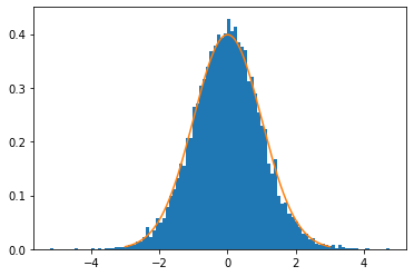
(a) $\sqrt{np_{2}k_{2}}\big{(}\widehat{\boldsymbol{R}}-c_{s}\mathring{\boldsymbol{R}}\big{)}_{10,1}/\widehat{s}_{10,1}$

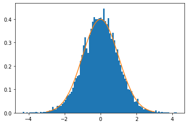
(b) $\sqrt{np_{2}k_{2}}\big{(}\widehat{\boldsymbol{R}}-c_{s}\mathring{\boldsymbol{R}}\big{)}_{19,3}/\widehat{s}_{19,3}$

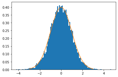
(c) $\sqrt{np_{1}k_{1}}\big{(}\widehat{\boldsymbol{C}}-r_{s}\mathring{\boldsymbol{C}}\big{)}_{3,1}/\widehat{s}_{3,1}^{\prime}$

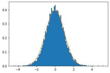
(d) $\sqrt{np_{1}k_{1}}\big{(}\widehat{\boldsymbol{C}}-r_{s}\mathring{\boldsymbol{C}}\big{)}_{13,2}/\widehat{s}_{13,2}^{\prime}$

Figure 1: Elementwise normality check for the estimated loadings $\widehat{}\boldsymbol{R}$ and $\widehat{}\boldsymbol{C}$ according to Theorem 9. The blue histograms are empirical densities, and the orange lines are the standard Gaussian density functions.

Next, we investigate the accuracy of the estimated factors, idiosyncratic variable, and FAMAR model coefficients. All experiments are repeated 100 times to reduce the effect of randomness. The simulations are carried out under two settings of parameters:

1. Fix $n=1000,\ n_{new}=1000,\ n^{\prime}=500,\ k_{1}=k_{2}=2,\ \operatorname{rank}(\boldsymbol{B}^{*})=2,$ and change $\ p_{1}=p_{2}$ in $\{20,30,40,50,60,70,80,90,100\}$.

2. Fix $p_{1}=80,\ p_{2}=50,\ n_{new}=1000,\ n^{\prime}=500,\ k_{1}=2,\ k_{2}=4,\ \operatorname{rank}(\boldsymbol{B}^{*})=2,$ and change $n$ in $\{500,1000,1500,2000,2500,3000,3500,4000,4500,5000\}$.

More settings of simulation exploration are available in Appendix I. For all cases, the true loading matrices $\boldsymbol{R}^{*}$ and $\boldsymbol{C}^{*}$ are generated element-wise from ${\cal N}(2,4)$. The true factors $\boldsymbol{F}_{i}$ and residuals $\boldsymbol{U}_{i}$ are generated such that each element is drawn from ${\cal N}(0,1)$ and ${\cal N}(0,0.04)$, respectively. Thereafter, the $\boldsymbol{X}_{i}$ are generated by the matrix factor model $\boldsymbol{X}_{i}=\boldsymbol{R}^{*}\boldsymbol{F}_{i}(\boldsymbol{C}^{*})^{\top}+\boldsymbol{U}_{i}$. For $\boldsymbol{B}^{*}$, we first generate a $p_{1}\times p_{2}$ matrix, with its individual elements sampled from ${\cal N}(0.5,0.25)$, and then we take its best low-rank ($\boldsymbol{B}^{*}$) approximation by SVD. The true response variables are defined by $y_{i}=\left\langle\boldsymbol{A}^{*},\boldsymbol{F}_{i}\right\rangle+\left\langle\boldsymbol{B}^{*},\boldsymbol{U}_{i}\right\rangle+\varepsilon_{i}$, where $\boldsymbol{A}^{*}:=0.5\cdot(\boldsymbol{R}^{*})^{\top}\boldsymbol{B}^{*}\boldsymbol{C}^{*}$ and $\varepsilon_{i}$ are drawn from ${\cal N}(0,1)$. By setting the variance of loading matrices much higher than that of the residual, we generate $\boldsymbol{X}_{i}$ with highly correlated rows and columns. The experiments are repeated 100 times to reduce the impact of randomness. The tuning parameter $\lambda$ for the nuclear norm penalty is chosen by cross-validation.

FAMAR Matrix Factor and Idiosyncratic Estimation.

Figures 2 and 3 plot the performance of the proposed algorithm in estimating $\boldsymbol{F}$ and $\boldsymbol{U}$ under Setting I. and Setting II., respectively. The estimation errors are all very small and decrease as either $n$ or $p_{1}$, $p_{2}$ increase, except that the error for $\widehat{\boldsymbol{F}}$ is not affected by increasing number of $n$ as it uses $n^{\prime}$ pre-training sample size. Those observations are consistent with our theoretical results. The comparison of the estimation on $\widehat{}\boldsymbol{U}$ with and without the block-averaging method showcases the privilege of the averaging algorithm.

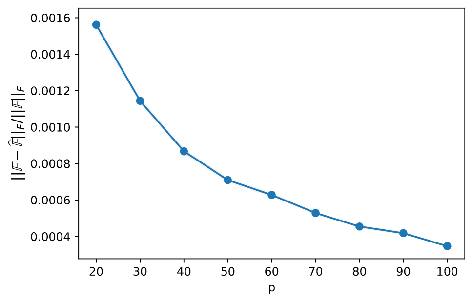
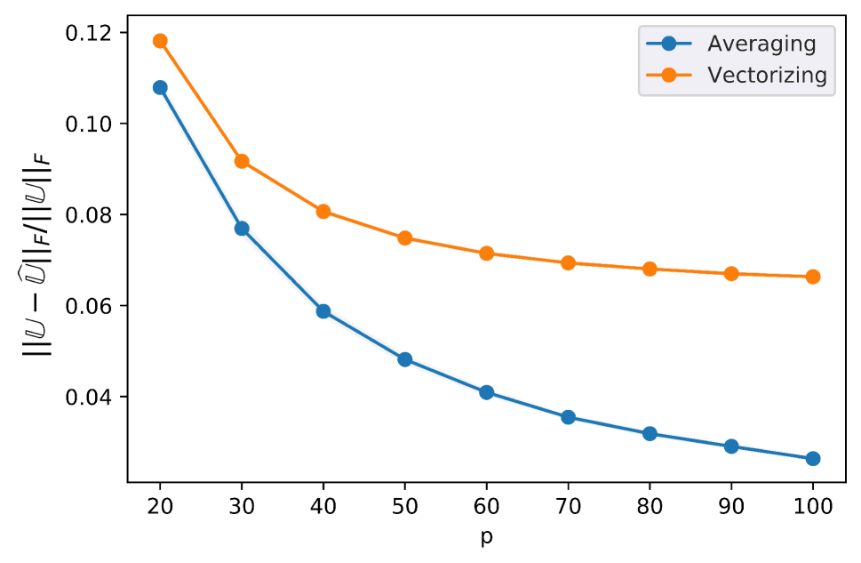
Figure 2: Performance of estimated $(\widehat{\boldsymbol{F}},\widehat{\boldsymbol{U}})$ under fixed $n=1000$ and increasing $p_{1}=p_{2}$ from $20$ to $100$. For factors, we report the relative error ${\|\mathbb{F}(\boldsymbol{H}_{2}\otimes\boldsymbol{H}_{1})^{\top}-\widehat{\mathbb{F}}\|_{F}}/{\|\mathbb{F}(\boldsymbol{H}_{2}\otimes\boldsymbol{H}_{1})^{\top}\|_{F}}$, where $\mathbb{F}\in\mathbb{R}^{n\times k_{1}k_{2}}$ is the matrix of vectorized true factors, and $\widehat{\mathbb{F}}$ is the estimation. For simplicity of notation, we omit the rotation matrix $\boldsymbol{H}_{2}\otimes\boldsymbol{H}_{1}$ in the figure label. Similar relative errors are reported for the estimation of idiosyncratic components, also comparing the performance with and without the block-average technique. The solid lines are the means among the 100 repetitions, the shadows show the standard deviations, and the vertical lines present the quartiles (which are too small to be visible on the graphs).

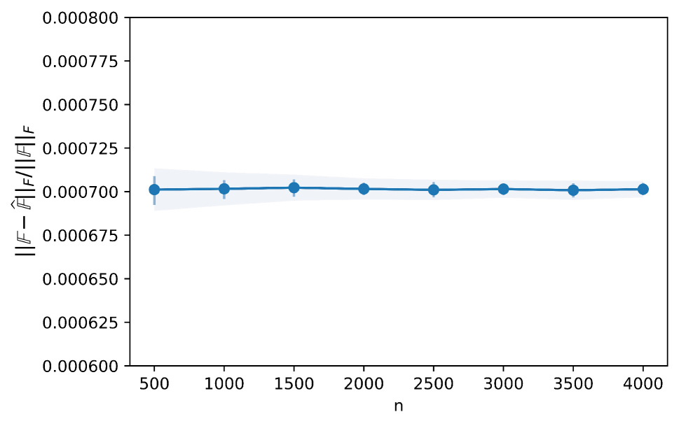
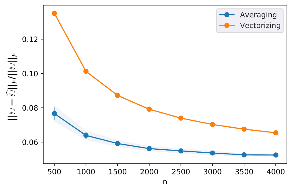
Figure 3: Performance of estimated $(\widehat{\mathbb{F}},\widehat{\mathbb{U}})$ when $n$ increases from $500$ to $4000$ with fixed $(p_{1},p_{2})=(70,50)$, The experiments are repeated 100 times. Labels are the same as that for Figure 2. The solid lines are the means, the shadows show the standard deviation, and the vertical lines present the quartiles. $\widehat{\mathbb{F}}$ is not affected by increasing number of $n$ as it uses $n^{\prime}$ pre-training sample size, which is consistent with Theorem 8.

FAMAR Coefficient Estimation and Prediction. Figures 4 and 5 compare our proposed FAMAR with two current benchmarks, namely, the vanilla matrix regression model (2) with nuclear penalty on $\boldsymbol{B}$, and the oracle factor augmented regression model (1) with observed $\boldsymbol{F}$ and $\boldsymbol{U}$, under Setting I. and Setting II., respectively. We could clearly see that our proposed FAMAR estimation tracks the performances of the oracle factor augmented regression closely in almost all tasks. Our proposed method outperforms the existing matrix regression with nuclear norm penalty in both estimation of coefficient $\boldsymbol{B}^{*}$ and prediction of new response $y$. Additionally, by generating a low-rank $\widehat{}\boldsymbol{B}$, as illustrated in the lower-right plots of Figures 4 and 5, FAMAR offers improved interpretability and stability compared to direct regression on $\boldsymbol{X}_{i}$’s. When the covariates $\boldsymbol{X}_{i}$ are highly correlated, applying low-rank regression directly to $\boldsymbol{X}_{i}$’s tends to overestimate the rank due to their dependency structure, which hampers the effectiveness of regularization and the interpretability of the model.

The superior performance of FAMAR stems from two key advantages. Firstly, since the space spanned by $(\boldsymbol{F}_{i},\boldsymbol{U}_{i})$ is identical to that spanned by $(\boldsymbol{F}_{i},\boldsymbol{X}_{i})$, FAMAR facilitates feature augmentation with $\boldsymbol{F}_{i}$, effectively leveraging latent information. Secondly, the factor model decorrelates the covariance matrix, resulting in more stable and interpretable coefficient estimators.

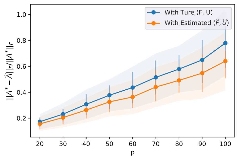
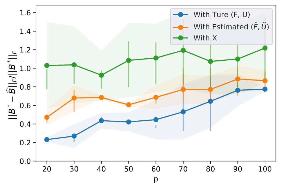
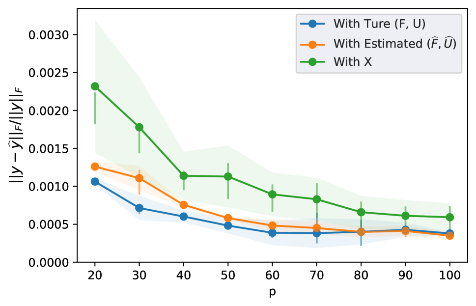
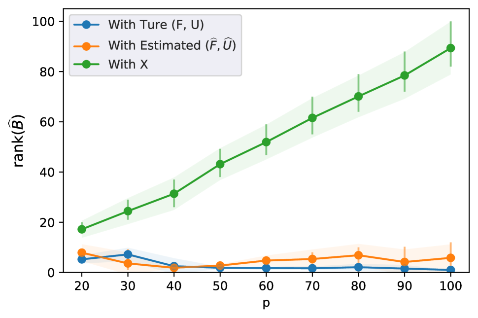
Figure 4: Fix $n=1000$, increase $p_{1}=p_{2}$ from $20$ to $100$. The blue, orange, and green lines correspond to running the regression with true $(\boldsymbol{F},\boldsymbol{U})$, estimated $(\widehat{\boldsymbol{F}},\widehat{\boldsymbol{U}})$, and $\boldsymbol{X}$, respectively. The solid lines are the means over 100 repetitions, the shadows show the standard deviation, and the vertical lines present the quartiles. The lower-right figure shows the rank of $\widehat{}\boldsymbol{B}$ with $\lambda$ chosen by cross-validation under different models.

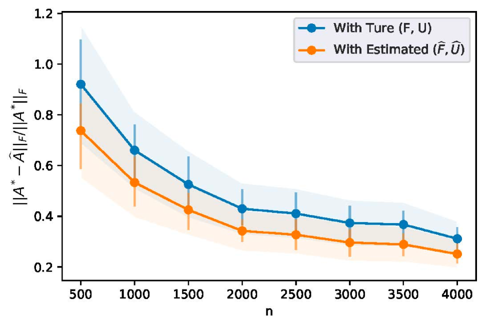
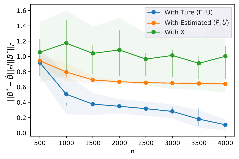
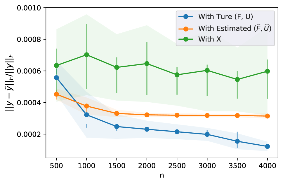
Figure 5: Fix $(p_{1},p_{2})=(70,50)$, increase $n$ from $500$ to $4000$. The blue, orange, and green lines correspond to doing the regression with true $(\boldsymbol{F},\boldsymbol{U})$, estimated $(\widehat{\boldsymbol{F}},\widehat{\boldsymbol{U}})$, and $\boldsymbol{X}$, respectively. The solid lines are the means over 100 repetitions, the shadows show the standard deviation, and the vertical lines present the quartiles.

5 Real Data Analysis

We demonstrate the advantages of FAMAR with an real application to the multinational macroeconomic indices collected from OECD (Chen et al., 2019). The dataset contains 10 quarterly macroeconomic indexes of 14 countries from 1990.Q4 to 2016.Q4 for 105 quarters. By implementing the proposed FAMAR, we accomplish various empirical objectives, including the prediction of economic indicators, extraction of economic factors, and estimation of factor impacts. Subsequent sections showcase the results.

Economic prediction. Here we showcase one-step ahead prediction of individual countries GDP using all the economic indicators from all countries in the last period. The covariate $\boldsymbol{X}_{i}$ is the $10$ (index) $\times 14$ (country) matrix in one quarter and the response $y_{i}$ is the GDP of a country of interest in the next quarter. We take the estimated factor dimension as $(k_{1},k_{2})=(4,4)$ according to the analysis in Chen & Fan (2021).

We use a rolling window to do a one-step ahead prediction on the GDP of the United States (USA), United Kingdom (GBR), France (FRA), and Germany (DEU). We set the window width as 68, the first $n^{\prime}=32$ samples of which are set to pre-train the projection matrices $\boldsymbol{W}_{1}$ and $\boldsymbol{W}_{2}$, while the following $n=36$ samples are used to estimate the loading matrices $\boldsymbol{R}^{*}$, $\boldsymbol{C}^{*}$ and the regression coefficient matrix $\boldsymbol{B}^{*}$. In each window, the covariate matrices $\boldsymbol{X}_{i}$ are normalized by subtracting the mean and dividing the standard deviation of the training set. The response variable $y_{i}$ is also demeaned by subtracting the sample mean of each training set.

The out-of-sample $R^{2}$ of GDP prediction on some representative countries are reported in Table 1. It is clear that FAMAR outperforms the vanilla matrix regression with a nuclear-norm penalty with much higher out-of-sample $R^{2}$. Besides the comparison with the baseline, we also present predictions based only on the estimated factors $\widehat{}\boldsymbol{F}_{i}$ or the estimated idiosyncratic components $\widehat{}\boldsymbol{U}_{i}$, respectively, to showcase their individual contributions to the process. As expected, it appears that factors play a predominant role in prediction, whereas the idiosyncratic components capture comparatively less valuable information in the context. This aligns with our expectation, for factors should capture most of the main and common features, and the residuals are regarded as idiosyncratic components corresponding to each feature, which are less representative and may vary a lot across time.

Table 1: Out-of-sample $R^{2}$ of predicting GDP

	FAMAR	$\widehat{}\boldsymbol{F}$	$\widehat{}\boldsymbol{U}+\|\boldsymbol{B}\|_{*}$	$\boldsymbol{X}+\|\boldsymbol{B}\|_{*}$
USA	0.1540	0.1751	-0.0512	-0.1066
GBR	0.2057	0.1727	0.0287	-0.0403
FRA	0.1961	0.1540	0.0789	-0.0411
DEU	0.1814	0.1460	0.1197	0.0050

Economic and Country Factors and Loadings. Figure 6 shows the heatmaps for estimates of the row and column loading matrices for the $4\times 4$ factor model. The loading matrices are normalized so that the $\ell_{2}$ norm of each column is one. They are also varimax-rotated to reveal a clear structure. From Figure 6(a) of the row factor loading matrix $\widehat{}\boldsymbol{R}$, we observed clearly that the rotated row factor 1-4 loaded heavily on central/western European, north American, Northern European, and Oceania countries, respectively. Accordingly, the four rotated row factors can be interpreted as the Central/Western European (C/W-EU), North American (NA), Northern European (N-EU), and Oceanian (OC) factors, mostly following geographical partitions. In a similar fashion, the four rotated column factors are (i) Economic output and industrial production (GDP&P); (ii) Consumer Price Index (CPI); (iii) International Trade (IT); (iv) Interest Rates (IR). Again, the factors agree with common economic knowledge.

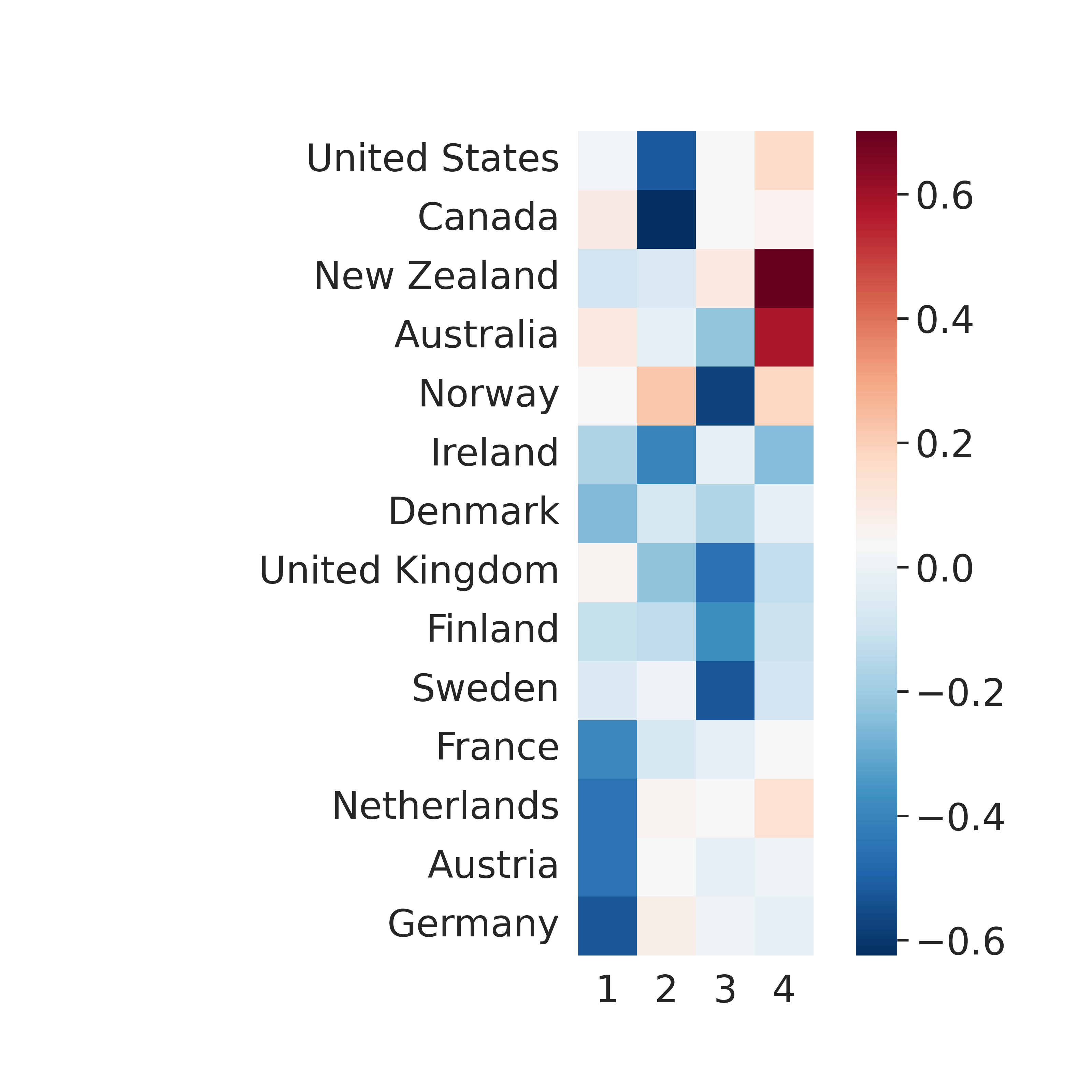
(a) $\widehat{}\boldsymbol{R}$ after varimax rotation

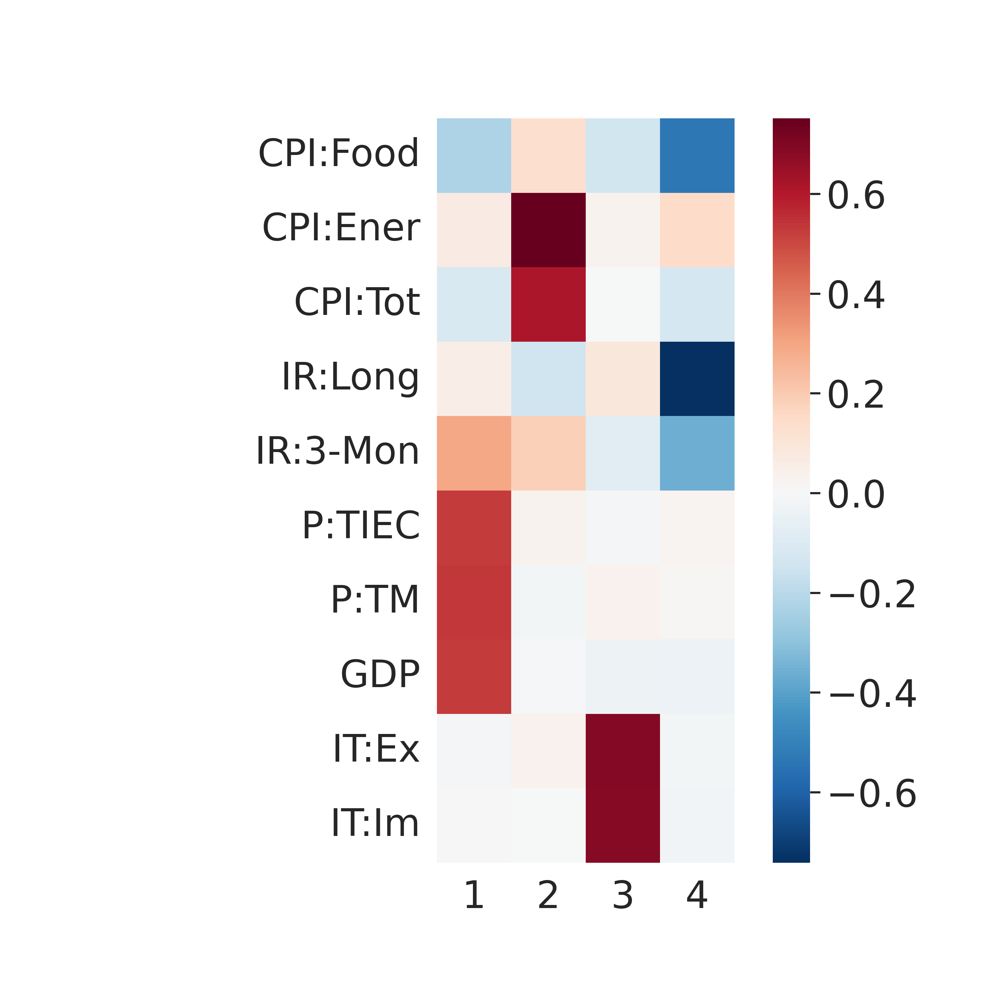
(b) $\widehat{}\boldsymbol{C}$ after varimax rotation

Figure 6: Estimations of row and column loading matrices (varimax rotated) of matrix factor model for multinational macroeconomic indices.

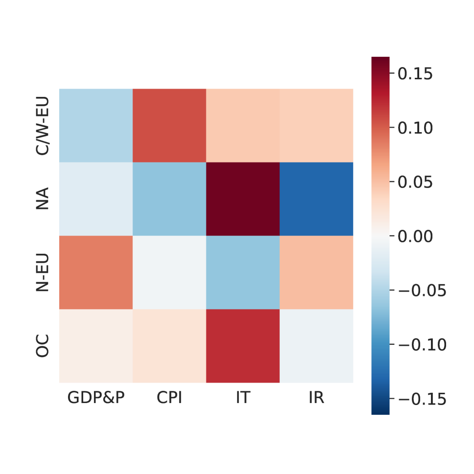
(a) USA

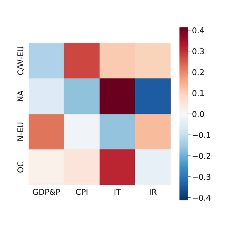
(b) GBR

(c) FRA

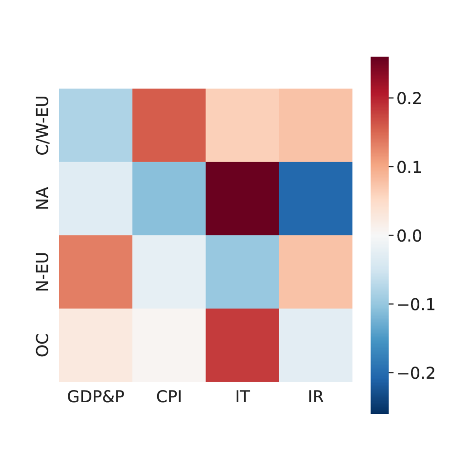
(d) DEU

Figure 7: Heatmap of $\widehat{}\boldsymbol{A}$ corresponding to the $\widehat{}\boldsymbol{F}_{i}$’s after rotation in Figure 6

Factors Impacts. To explore the impact of latent factors on the GDP of different countries, Figure 7 presents the heat map of $\widehat{}\boldsymbol{A}$ over the period. The heatmaps of $\widehat{}\boldsymbol{A}$ exhibit notable similarities across the four examined countries. A discernible pattern reveals several coordinates characterized by substantial magnitudes. Specifically, the four most significant coefficients, in terms of magnitude, correspond to the pairs: (IT, NA), (IR, NA), (IT, OC), and (CPI, C/W-EU). This implies that international trade and interest rates in North America, international trade in Oceania, and the CPI of Central and Western Europe play pivotal roles in forecasting the GDP of the countries.

6 Conclusion

We introduce Factor-Augmented Matrix Regression (FAMAR) as a powerful framework to tackle the growing complexity of matrix-variate data and its inherent high-dimensionality challenges. FAMAR comprises two pivotal algorithms, each designed to address distinct aspects of the problem. The first algorithm presents an innovative, non-iterative approach that efficiently estimates the factors and loadings within the matrix factor model. Leveraging advanced techniques such as pre-training, diverse projection, and block-wise averaging, it streamlines the estimation process. The second algorithm, equally crucial, offers an accelerated solution for nuclear-norm penalized matrix factor regression. Both algorithms are underpinned by robust statistical and numerical convergence guarantees, ensuring their reliability in practical applications.

Empirical assessments across a range of synthetic and real datasets substantiate the efficacy of FAMAR. Notably, it outperforms existing methods in terms of prediction accuracy, factor interpretability, and computational efficiency. FAMAR’s versatility and superior performance make it a valuable addition to the toolkit of researchers and practitioners working with matrix-variate data. Its potential applications extend across diverse domains, from economics and finance to machine learning and data mining, where handling high-dimensional matrix data efficiently and effectively is paramount. As we move forward in the era of big data, FAMAR stands as a testament to the ongoing innovation in statistical modeling and data analysis, promising new avenues for extracting valuable insights from complex datasets.

Appendix A Notations

We use the notation $[N]$ to refer to the positive integer set $\left\{1,\ldots,N\right\}$ for $N\in\mathbb{Z}_{+}$. For any matrix $\boldsymbol{X}$, we use $\boldsymbol{x}_{i\cdot}$, $\boldsymbol{x}_{j}$, and $x_{ij}$ to refer to its $i$-th row, $j$-th column, and $ij$-th entry, respectively. All vectors are column vectors and row vectors are written as $\boldsymbol{x}^{\top}$ for any vector $\boldsymbol{x}$. For any two scalers $p$, $q$, we denote $p\wedge q:=\min\{p,q\}$ and $p\vee q:=\max\{p,q\}$.

We use $\operatorname{vec}(\boldsymbol{X})$ as the vectorization of $\boldsymbol{X}$ and use $\mathbb{X}$ to denote a matrix whose rows are specifically vectorized matrices. That is, the $i$-th row of $\mathbb{X}$ is $\operatorname{vec}(\boldsymbol{X}_{i})^{\top}$. For two matrices $\boldsymbol{X}_{1}\in\mathbb{R}^{m\times n}$ and $\boldsymbol{X}_{2}\in\mathbb{R}^{p\times q}$, $\boldsymbol{X}_{1}\otimes\boldsymbol{X}_{2}\in\mathbb{R}^{pm\,\times\,qn}$ is the Kronecker product. Note that $\operatorname{vec}(\boldsymbol{A}\boldsymbol{X}\boldsymbol{B})=(\boldsymbol{B}^{\top}\otimes\boldsymbol{A})\operatorname{vec}(\boldsymbol{X})$. We denote $\operatorname{diag}(\boldsymbol{X}_{1},\boldsymbol{X}_{2})\in\mathbb{R}^{(m+p)\times(n+q)}$ as the block-diagonal matrix with $\boldsymbol{X}_{1}$ and $\boldsymbol{X}_{2}$ being its diagonal blocks.

For any vector $\boldsymbol{x}=(x_{1},\ldots,x_{p})^{\top}$, we let $\|\boldsymbol{x}\|:=\|\boldsymbol{x}\|_{2}=(\sum_{i=1}^{p}x_{i}^{2})^{1/2}$ be the $\ell_{2}$-norm, and let $\|\boldsymbol{x}\|_{1}=\sum_{i=1}^{p}|x_{i}|$ be the $\ell_{1}$-norm. Besides, we use the following matrix norms: $\ell_{2}$-norm $\left\lVert\boldsymbol{X}\right\rVert_{2}:=\sigma_{max}(\boldsymbol{X})$; $(2,1)$-norm $\left\lVert\boldsymbol{X}\right\rVert_{2,1}:=\underset{\left\lVert\boldsymbol{a}\right\rVert_{1}=1}{\max}\left\lVert\boldsymbol{X}\boldsymbol{a}\right\rVert_{2}=\max_{i}\left\lVert\boldsymbol{x}_{i}\right\rVert_{2}$; Frobenius norm $\|\boldsymbol{X}\|_{F}=(\sum_{i,j}x_{ij}^{2})^{1/2}$; nuclear norm $\|\boldsymbol{X}\|_{*}=\sum_{i=1}^{n}{\sigma_{i}(\boldsymbol{X})}$. When $\boldsymbol{X}$ is a square matrix, we denote by $\operatorname{Tr}\left(\boldsymbol{X}\right)$, $\lambda_{max}\left(\boldsymbol{X}\right)$, and $\lambda_{min}\left(\boldsymbol{X}\right)$ the trace, maximum and minimum singular value of $\boldsymbol{X}$, respectively. For two matrices of the same dimension, define the inner product $\left\langle\boldsymbol{X}_{1},\boldsymbol{X}_{2}\right\rangle=\operatorname{Tr}(\boldsymbol{X}_{1}^{\top}\boldsymbol{X}_{2})$.

Appendix B Computation

B.1 Explanation of the Accelerated Algorithm

To elucidate the accelerated algorithm, we first consider the vanilla gradient algorithm with the gradient step performed at the approximate solution $\{(\boldsymbol{A}^{(k)},\boldsymbol{B}^{(k)})\}$, which consists of a singular value thresholding (SVT) on the gradient step of estimating $\boldsymbol{B}^{*}$ and a regular update of $\boldsymbol{A}^{*}$. The partial gradient of $f_{n}$ with respect to $\boldsymbol{B}$ is

$$\nabla_{B}f_{n}(\boldsymbol{A},\boldsymbol{B})=-\frac{1}{n}\sum_{i=1}^{n}\left(y_{i}-\left\langle\boldsymbol{A},\boldsymbol{F}_{i}\right\rangle-\left\langle\boldsymbol{B},\boldsymbol{U}_{i}\right\rangle\right)\boldsymbol{U}_{i}.$$

Both $\nabla_{A}f_{n}(\boldsymbol{A},\boldsymbol{B})$ and $\nabla_{B}f_{n}(\boldsymbol{A},\boldsymbol{B})$ are $L$-Lipschitz with given $\{(\boldsymbol{F}_{i},\boldsymbol{U}_{i})\}_{i=1}^{n}$. Given a prescribed precision level $\epsilon$ and some initialization $\boldsymbol{A}^{(0)}$ and $\boldsymbol{B}^{(0)}$, we can estimate $\boldsymbol{A}^{*}$ and $\boldsymbol{B}^{*}$ alternatively. Given $\boldsymbol{A}^{(k-1)}$, $\boldsymbol{B}^{(k-1)}$ and the step size $L^{(k)}$, $\boldsymbol{B}$ can be updated by:

$$\boldsymbol{B}^{(k)}=\operatorname*{argmin}_{\boldsymbol{B}}\left\{\frac{L^{(k)}}{2}\left\lVert\boldsymbol{B}-\left(\boldsymbol{B}^{(k-1)}-\frac{1}{L^{(k)}}\nabla_{B}f_{n}(\boldsymbol{A}^{(k-1)},\boldsymbol{B}^{(k-1)})\right)\right\rVert_{F}^{2}+\lambda_{n}\left\lVert\boldsymbol{B}\right\rVert_{*}\right\},$$ (25)

which admits an analytic solution

$$\boldsymbol{B}^{(k)}={\cal T}_{\lambda_{n}/L^{(k)}}\left(\boldsymbol{B}^{(k-1)}-\frac{1}{L^{(k)}}\nabla_{B}f_{n}(\boldsymbol{A}^{(k-1)},\boldsymbol{B}^{(k-1)})\right):=p_{L^{(k)}}(\boldsymbol{A}^{(k-1)},\boldsymbol{B}^{(k-1)}),$$ (26)

where ${\cal T}_{\lambda}(\boldsymbol{C})$ is an operator defined as ${\cal T}_{\lambda}(\boldsymbol{C})=\boldsymbol{U}\boldsymbol{D}_{\lambda}\boldsymbol{V}^{\top}$ on a matrix $\boldsymbol{C}$ with SVD $\boldsymbol{C}=\boldsymbol{U}\boldsymbol{D}\boldsymbol{V}^{\top}$ and $\boldsymbol{D}_{\lambda}$ is diagonal with the soft thresholding $(d_{\lambda})_{ii}=\operatorname{sign}(d_{ii})\max\{0,\left\lvert d_{ii}\right\rvert-\lambda\}$. Since $\boldsymbol{A}$ is of low dimension, it can be updated directly by gradient descent:

$$\boldsymbol{A}^{(k)}=q_{L^{(k)}}(\boldsymbol{A}^{(k-1)},\boldsymbol{B}^{(k-1)}):=\boldsymbol{A}^{(k-1)}-\frac{1}{L^{(k)}}\nabla_{A}f_{n}(\boldsymbol{A}^{(k-1)},\boldsymbol{B}^{(k-1)}).$$ (27)

The accelerated algorithm performs the gradient step at the search point $\{(\boldsymbol{Q}^{(k)},\boldsymbol{P}^{(k)})\}$. So $\boldsymbol{A}^{(k)}$ and $\boldsymbol{B}^{(k)}$ are calculated according to equation (26) and (27) with $(\boldsymbol{A}^{(k-1)},\boldsymbol{B}^{(k-1)})$ replaced by the search point $(\boldsymbol{Q}^{(k)},\boldsymbol{P}^{(k)})$.

B.2 Numerical Convergence

Lemma 17.

Given $\boldsymbol{A}^{(k-1)}$, $\boldsymbol{B}^{(k-1)}$ and the step size $L^{(k)}$, $\boldsymbol{B}$ can be updated by:

$$\boldsymbol{B}^{(k)}=\operatorname*{argmin}_{\boldsymbol{B}}\left\{\frac{L^{(k)}}{2}\left\lVert\boldsymbol{B}-\left(\boldsymbol{B}^{(k-1)}-\frac{1}{L^{(k)}}\nabla_{B}f_{n}(\boldsymbol{A}^{(k-1)},\boldsymbol{B}^{(k-1)})\right)\right\rVert_{F}^{2}+\lambda_{n}\left\lVert\boldsymbol{B}\right\rVert_{*}\right\},$$ (28)

or, equivalently,

$$\boldsymbol{B}^{(k)}=p_{L^{(k)}}(\boldsymbol{A}^{(k-1)},\boldsymbol{B}^{(k-1)}):={\cal T}_{\lambda_{n}/L^{(k)}}\left(\boldsymbol{B}^{(k-1)}-\frac{1}{L^{(k)}}\nabla_{B}f_{n}(\boldsymbol{A}^{(k-1)},\boldsymbol{B}^{(k-1)})\right),$$ (29)

where ${\cal T}_{\lambda}(\boldsymbol{C})$ is an operator defined as ${\cal T}_{\lambda}(\boldsymbol{C})=\boldsymbol{U}\boldsymbol{D}_{\lambda}\boldsymbol{V}^{\top}$ on a matrix $\boldsymbol{C}$ with SVD $\boldsymbol{C}=\boldsymbol{U}\boldsymbol{D}\boldsymbol{V}^{\top}$ and $\boldsymbol{D}_{\lambda}$ is diagonal with $(d_{\lambda})_{ii}=\operatorname{sign}(d_{ii})\max\{0,\left\lvert d_{ii}\right\rvert-\lambda\}$.

Proof of Lemma 17.

Lemma 17 can be prove by invoking Theorem 2.1 in (Cai et al. 2010). ∎

Lemma 18.

Let

$$p_{L}(\boldsymbol{A},\boldsymbol{B})=\operatorname*{argmin}_{\boldsymbol{B}^{\prime}}\big{\{}H_{L,B}(\boldsymbol{B}^{\prime};\boldsymbol{A},\boldsymbol{B})+\lambda_{n}\|\boldsymbol{B}^{\prime}\|_{*}\big{\}},\quad q_{L}(\boldsymbol{A},\boldsymbol{B})=\operatorname*{argmin}_{\boldsymbol{A}^{\prime}}H_{L,A}(\boldsymbol{A}^{\prime};\boldsymbol{A},\boldsymbol{B}),$$

where

$$H_{L,A}(\boldsymbol{A}^{\prime};\boldsymbol{A},\boldsymbol{B}) :=\left\langle\boldsymbol{A}^{\prime}-\boldsymbol{A},\nabla_{A}f_{n}(\boldsymbol{A},\boldsymbol{B})\right\rangle+\frac{L}{2}\|\boldsymbol{A}^{\prime}-\boldsymbol{A}\|_{F}^{2},$$ (30)

$$H_{L,B}(\boldsymbol{B}^{\prime};\boldsymbol{A},\boldsymbol{B}) :=\left\langle\boldsymbol{B}^{\prime}-\boldsymbol{B},\nabla_{B}f_{n}(\boldsymbol{A},\boldsymbol{B})\right\rangle+\frac{L}{2}\|\boldsymbol{B}^{\prime}-\boldsymbol{B}\|_{F}^{2}.$$ (31)

Assume the following inequality holds:

$$F_{n}\big{(}p_{L}(\boldsymbol{A},\boldsymbol{B}),p_{L}(\boldsymbol{A},\boldsymbol{B})\big{)}\geq f_{n}(\boldsymbol{A},\boldsymbol{B})+H_{L,B}(p_{L}(\boldsymbol{A},\boldsymbol{B});\boldsymbol{A},\boldsymbol{B})$$ (32)

$$+H_{L,A}(q_{L}(\boldsymbol{A},\boldsymbol{B});\boldsymbol{A},\boldsymbol{B})+\lambda_{n}\|p_{L}(\boldsymbol{A},\boldsymbol{B})\|_{*}.$$

Then for any $\boldsymbol{B}^{\prime}\in\mathbb{R}^{p_{1}\times p_{2}}$ and $\boldsymbol{A}^{\prime}\in\mathbb{R}^{k_{1}\times k_{2}}$, we have

$$F_{n}\big{(}\boldsymbol{A}^{\prime},\boldsymbol{B}^{\prime}\big{)}-F_{n}\big{(}q_{L}(\boldsymbol{A},\boldsymbol{B}), \ p_{L}(\boldsymbol{A},\boldsymbol{B})\big{)}\geq\frac{L}{2}\big{(}\|p_{L}(\boldsymbol{A},\boldsymbol{B})-\boldsymbol{B}\|_{F}^{2}+\|q_{L}(\boldsymbol{A},\boldsymbol{B})-\boldsymbol{A}\|_{F}^{2}\big{)}$$ (33)

$$+L\big{(}\left\langle\boldsymbol{B}-\boldsymbol{B}^{\prime},p_{L}(\boldsymbol{A},\boldsymbol{B})-\boldsymbol{B}\right\rangle+\left\langle\boldsymbol{A}-\boldsymbol{A}^{\prime},q_{L}(\boldsymbol{A},\boldsymbol{B})-\boldsymbol{A}\right\rangle\big{)}.$$

Further, let $\{(\boldsymbol{A}^{(k)},\boldsymbol{B}^{(k)})\}_{k\geq 1}$ be the sequences generated by Algorithm 1. Then for any $k\geq 1$, we have

$$F_{n}(\boldsymbol{A}^{(k)},\boldsymbol{B}^{(k)})-F_{n}(\boldsymbol{A}^{*},\boldsymbol{B}^{*})\leq\frac{2\gamma L\big{(}\|\boldsymbol{A}^{(0)}-\boldsymbol{A}^{*}\|_{F}^{2}+\|\boldsymbol{B}^{(0)}-\boldsymbol{B}^{*}\|_{F}^{2}\big{)}}{(k+1)^{2}}.$$ (34)

Proof.

The $p_{L}(\boldsymbol{A},\boldsymbol{B})$ and $q_{L}(\boldsymbol{A},\boldsymbol{B})$ defined in Lemma 18 is equivalent to that defined in Section 2.2, which can be shown using Lemma 17 and Bertsekas et al. (1999), see also equation (5)-(7) in Ji & Ye (2009). The global convergence rate of Algorithm 1 is established by Lemma 18, whose proves are direct extensions of Theorem 4.1 in Ji & Ye (2009) and are therefore omitted. ∎

Appendix C Technical Assumptions

The following assumptions are needed for technical purposes. Assumption 19 and 20 imposes conditions on factors and idiosyncratic components, still allowing weak correlations. Assumption 21 is already satisfied by the data-driven method we have studied by its construction and by Proposition 7. Nevertheless, since some other reasonable projection matrices can also be used, we impose Assumption 21 for genreality. Assumption 22 is needed for asymptotic normality.

Assumption 19.

For MFM (1), there exists universal constants $c_{0}$ and $c_{1}$ such that

1. The elements of $\boldsymbol{F}_{i}\in\mathbb{R}^{k_{1}\times k_{2}}$ are mean zero, sub-Gaussian, and weakly correlated in the sense that: $\boldsymbol{F}_{i}=\boldsymbol{\Sigma}_{k_{1}}\boldsymbol{Z}_{i}\boldsymbol{\Sigma}_{k_{2}}$, where $\boldsymbol{Z}_{i}\in\mathbb{R}^{k_{1}\times k_{2}}$ has independent mean zero sub-Gaussian entries, and for $\boldsymbol{\Sigma}_{k_{1}}\in\mathbb{R}^{k_{1}\times k_{1}}$, $\boldsymbol{\Sigma}_{k_{2}}\in\mathbb{R}^{k_{2}\times k_{2}}$, assume that $0<\|\boldsymbol{\Sigma}_{k_{j}}\|_{2}<c_{0}$ for $j=1,2$.

2. The elements of $\boldsymbol{U}_{i}\in\mathbb{R}^{p_{1}\times p_{2}}$ are mean zero, sub-Gaussian, and weakly correlated in the same sense as above. Furthermore, assume that

   $$\text{for }i,k\in[p_{1}],i\neq k,\mathbb{E}\left[\sum_{j=1}^{p_{2}}u_{ij}u_{kj}\right]\leq c_{1}\sqrt{\frac{p_{2}}{p_{1}}};$$

   $$\text{and for }i,k\in[p_{2}],i\neq k,\mathbb{E}\left[\sum_{j=1}^{p_{1}}u_{ji}u_{jk}\right]\leq c_{1}\sqrt{\frac{p_{1}}{p_{2}}}.$$

Assumption 20.

There exist universal constants $c_{1},c_{2}$, and $C_{2}$ such that

1. $\frac{1}{n}\sum_{i=1}^{n}\sum_{j=1}^{n}\mathbb{E}\|\boldsymbol{F}_{j}\|_{F}\|\boldsymbol{F}_{i}\|_{F}\operatorname{Tr}\left(\mathbb{E}\left[\boldsymbol{U}_{j}\boldsymbol{U}_{i}^{\top}\mid\boldsymbol{F}\right]\right)<c_{1}.$

2. $c_{2}<\lambda_{\min}(\mathbb{F}^{\top}\mathbb{F}/n)<\lambda_{\max}(\mathbb{F}^{\top}\mathbb{F}/n)<C_{2}$, and $\sum_{i=1}^{n}\widetilde{}\boldsymbol{f}_{i}\widetilde{}\boldsymbol{f}_{i}^{\top}\xrightarrow{P}\boldsymbol{\Sigma}_{F}$ for some $k_{1}\!k_{2}\times k_{1}\!k_{2}$ positive definite matrix $\boldsymbol{\Sigma}_{F}$, where $\widetilde{\boldsymbol{f}}_{i}:=\operatorname{vec}(\boldsymbol{F}_{i})$ and $\mathbb{F}=\big{(}\widetilde{\boldsymbol{f}}_{1}\cdots\widetilde{\boldsymbol{f}}_{n}\big{)}^{\top}$.

Assumption 21.

There exist universal constants $c_{1},c_{2}$, $C_{1}$, and $C_{2}$ such that

1. $\nu_{\max}(\boldsymbol{H}_{i})\leq C_{i}\nu_{\min}(\boldsymbol{H}_{i})$, for $i=1,2$.

2. $\lambda_{\min}(\boldsymbol{W}_{i}^{\top}\boldsymbol{W}_{i}/p_{i})\geq c_{i}$, for $i=1,2$.

Assumption 22.

1. There exists a constant $M<\infty$ such that the $k_{1}\!k_{2}\times k_{1}\!k_{2}$ matrix satisfies

   $$\mathbb{E}\left\|\frac{1}{np_{1}\!p_{2}}\sum_{i=1}^{n}\sum_{j=1}^{p_{1}\!p_{2}}[\boldsymbol{W}_{2}^{\top}\otimes\boldsymbol{W}_{1}^{\top}]_{j}\widetilde{\boldsymbol{f}}_{i}^{\top}\widetilde{u}_{ij}\right\|^{2}\leq M,$$

   where $[\boldsymbol{W}_{2}^{\top}\otimes\boldsymbol{W}_{1}^{\top}]_{j}$ is the $j$-th column of $(\boldsymbol{W}_{2}^{\top}\otimes\boldsymbol{W}_{1}^{\top})$, $\widetilde{}\boldsymbol{f}_{i}^{\top}$ is the $i$-th row of $\mathbb{F}$, and $\widetilde{u}_{ij}$ is the $(i,j)$-th element of $\mathbb{U}$.

2. There exists a full-rank $k_{1}\!k_{2}\times k_{1}k_{2}$ matrix $\boldsymbol{\Lambda}_{H}$ such that

   $$\operatorname*{\mathit{p}lim}_{p_{1},p_{2}\rightarrow\infty}(\boldsymbol{H}_{2}\otimes\boldsymbol{H}_{1})=\boldsymbol{\Lambda}_{H}.$$

   This also implies $\nu_{\min}(\boldsymbol{H}_{i}),\nu_{\max}(\boldsymbol{H}_{i})=\Omega_{p}(1)$, for $i=1,2$.

3. There exists an $k_{1}\!k_{2}\times k_{1}\!k_{2}$ matrix $\boldsymbol{\Sigma}_{U}$ such that

   $$\lim_{p_{1},p_{2}\rightarrow\infty}\frac{1}{p_{1}\!p_{2}}\sum_{j=1}^{p_{1}\!p_{2}}\sum_{k=1}^{p_{1}\!p_{2}}[\boldsymbol{W}_{2}^{\top}\otimes\boldsymbol{W}_{1}^{\top}]_{j}[\boldsymbol{W}_{2}^{\top}\otimes\boldsymbol{W}_{1}^{\top}]_{k}^{\top}\mathbb{E}[\widetilde{u}_{ij}\widetilde{u}_{ik}]=\boldsymbol{\Sigma}_{U},\text{ for }i\in[n].$$

4. Assume that there exist a $k_{1}\!k_{2}\times k_{1}\!k_{2}$ matrix $\boldsymbol{\Phi}$ and a $p_{1}\!p_{2}\times p_{1}\!p_{2}$ matrix $\boldsymbol{\Psi}$ such that

   $$\frac{1}{\sqrt{n}}\sum_{i=1}^{n}\widetilde{\boldsymbol{f}}_{i}\widetilde{\boldsymbol{u}}_{i}^{\top}\xrightarrow[]{d}{\cal M}{\cal N}(\boldsymbol{0},\boldsymbol{\Phi},\boldsymbol{\Psi}),$$

   where $\widetilde{\boldsymbol{u}}_{i}=\operatorname{vec}(\boldsymbol{U}_{i})$, $\boldsymbol{\Psi}$ is divided into $p_{2}\times p_{2}$ blocks, denoted as $\boldsymbol{\Psi}_{ij}\in\mathbb{R}^{p_{1}\times p_{1}}$, for $i,j\in[p_{2}]$, and that $\boldsymbol{\Psi}_{ij}={\rm o_{p}}\left(p^{-1}\right)$ for all $i\neq j$.

5. There exists $M\leq\infty$ such that for all $n$, $p_{1},$ and $p_{2}$, $\mathbb{E}\widetilde{u}_{ij}=0$, $\mathbb{E}|\widetilde{u}_{ij}|^{8}\leq M$.

Appendix D Theoretical Analysis of “Pre-trained Projection” and “Block-wise Averaging”

D.1 Proof of Proposition 7

We denote $\boldsymbol{S}^{*}_{1}=\frac{1}{p_{1}}\boldsymbol{R}^{*}{\boldsymbol{R}^{*}}^{\top}$, $\boldsymbol{S}^{*}_{2}=\frac{1}{p_{2}}\boldsymbol{C}^{*}{\boldsymbol{C}^{*}}^{\top}$, $\widehat{\boldsymbol{S}}_{1}=\frac{1}{p_{1}p_{2}n}\sum_{i=1}^{n}{\boldsymbol{X}_{i}\boldsymbol{X}_{i}^{\top}}$, and $\widehat{}\boldsymbol{S}_{2}=\frac{1}{p_{1}p_{2}n}\sum_{i=1}^{n}{\boldsymbol{X}_{i}^{\top}\boldsymbol{X}_{i}}$. We first present a technical lemma that bounds the $\ell_{2}$ norm between $\widehat{\boldsymbol{S}}_{1}$ (resp. $\widehat{}\boldsymbol{S}_{2}$) and $\boldsymbol{S}^{*}_{1}$ (resp. $\boldsymbol{S}^{*}_{2}$). Its proof is provided at the end of this section.

Lemma 23.

Under Assumption 5 and 19, there exists a universal constant $c$ such that

$$\left\|\widehat{\boldsymbol{S}}_{1}-\boldsymbol{S}^{*}_{1}\right\|_{2}\leq c\left(\sqrt{t(k_{1}\vee k_{2})}\sqrt{\frac{\log k_{1}+t}{n}}+\frac{1}{\sqrt{p_{1}}}\right),$$

and

$$\left\|\widehat{}\boldsymbol{S}_{2}-\boldsymbol{S}^{*}_{2}\right\|_{2}\leq c\left(\sqrt{t(k_{1}\vee k_{2})}\sqrt{\frac{\log k_{2}+t}{n}}+\frac{1}{\sqrt{p_{2}}}\right)$$

with probability at least $1-11e^{-t}$

Proof of Proposition 7.

Since the proof for $\boldsymbol{H}_{1}$ and $\boldsymbol{H}_{2}$ are the same, we only provide that for $\boldsymbol{H}_{1}$ as follows. The argument below is deterministic, conditioned on the event in Lemma 23.

Let $\widehat{\boldsymbol{Z}}\in\mathbb{R}^{p_{1}\times k_{1}}$ be the matrix consists of the top $k_{1}$ top eigenvectors of $\widehat{\boldsymbol{S}}_{1}$. Then $\boldsymbol{W}_{1}=\sqrt{p_{1}}\widehat{\boldsymbol{Z}}$. Since $\boldsymbol{S}^{*}_{1}$ is symmetric, it has the eigen decomposition $\boldsymbol{S}^{*}_{1}=\boldsymbol{Z}^{*}\boldsymbol{\Lambda}^{*}{\boldsymbol{Z}^{*}}^{\top}$, where $\boldsymbol{\Lambda}^{*}$ is a $k_{1}\times k_{1}$ diagonal matrix, and $\boldsymbol{Z}^{*}\in\mathbb{R}^{p_{1}\times k_{1}}$ satisfies ${\boldsymbol{Z}^{*}}^{\top}\boldsymbol{Z}^{*}=\boldsymbol{I}_{k_{1}}$. Hence, $\boldsymbol{R}^{*}=\boldsymbol{Z}^{*}{\boldsymbol{\Lambda}^{*}}^{1/2}$. The upper bound is derived from

$$\nu_{\max}\left(\frac{1}{p_{1}}\boldsymbol{W}_{1}^{\top}\boldsymbol{R}^{*}\right) =\sup_{\boldsymbol{u}\in\SS^{k_{1}-1}}\left\|\frac{1}{p_{1}}{\boldsymbol{R}^{*}}^{\top}\boldsymbol{W}_{1}\boldsymbol{u}\right\|_{2}\leq\frac{1}{\sqrt{p_{1}}}\left\|{\boldsymbol{\Lambda}^{*}}^{1/2}\right\|\sup_{\boldsymbol{u}\in\SS^{k_{1}-1}}\left\|{\boldsymbol{Z}^{*}}^{\top}\widehat{\boldsymbol{Z}}\boldsymbol{u}\right\|_{2}$$

$$\leq C_{1}\sup_{\boldsymbol{u}\in\SS^{k_{1}-1}}\left\|{\boldsymbol{Z}^{*}}^{\top}\widehat{\boldsymbol{Z}}\boldsymbol{u}\right\|_{2}\leq C_{1}\sup_{\boldsymbol{u}\in\SS^{k_{1}-1}}\left\|\boldsymbol{u}\right\|_{2}=C_{1}$$

for some universal positive constant $C_{1}$, where the second inequality is because of Assumption 6.

As for the lower bound, we have

$$\nu_{\min}\left(\frac{1}{p_{1}}\boldsymbol{W}_{1}^{\top}\boldsymbol{R}^{*}\right)\geq\frac{1}{\sqrt{p_{1}}}\nu_{\min}\left(\widehat{\boldsymbol{Z}}\boldsymbol{Z}^{*}\right)\nu_{\min}\left({\boldsymbol{\Lambda}^{*}}^{1/2}\right)\geq c_{1}\nu_{\min}\left(\widehat{\boldsymbol{Z}}\boldsymbol{Z}^{*}\right),$$ (35)

where the last inequality follows from Assumption 6. Let $\lambda_{1},\ldots,\lambda_{p_{1}}$ be the eigenvalues of $\boldsymbol{S}^{*}_{1}$ in the non-decreasing order, and let $\widehat{\lambda}_{1},\ldots,\widehat{\lambda}_{p_{1}}$ be the eigenvalues of $\widehat{\boldsymbol{S}}_{1}$ in the non-decreasing order. Then by Assumption 6 and that $\operatorname{rank}(\boldsymbol{S})=k_{1}$, we have

$$\lambda_{k_{1}}\geq c_{1}\text{ for some constant }c_{1},\text{ and }\lambda_{k_{1}+1}=0.$$ (36)

Let $\delta:=\sqrt{t(k_{1}\vee k_{2})}\sqrt{\frac{\log k_{1}+t}{n}}+\frac{1}{\sqrt{p_{1}}}$. By Weyl’s Theorem and Lemma 23, there exists a universal constant $c_{2}$ such that

$$\left|\widehat{\lambda}_{i}-\lambda_{i}\right|\leq\left\|\widehat{\boldsymbol{S}}_{1}-\boldsymbol{S}^{*}_{1}\right\|_{2}\leq c_{2}\delta,\text{ for all }i\in[p_{1}].$$ (37)

with probability at least $1-11e^{-t}$.

We argue that

$$\nu_{\min}\left(\widehat{\boldsymbol{Z}}\boldsymbol{Z}^{*}\right)\geq\sqrt{1-\left(\frac{2c_{2}}{c_{1}}\delta\right)^{2}}\geq 1-\frac{2c_{2}}{c_{1}}\delta.$$

It suffices to prove the above inequality for $\delta<c_{1}/(2c_{2})$; otherwise, the inequality is trivial. In this case, combining (36) and (37), we bound the eigen-gap between $\widehat{\boldsymbol{S}}_{1}$ and $\boldsymbol{S}^{*}_{1}$ by

$$\widetilde{\delta}:= \inf\left\{|\lambda-\widehat{\lambda}|\mid\lambda\in[\lambda_{k_{1}},\lambda_{1}],\widehat{\lambda}\in(-\infty,\widehat{\lambda}_{k_{1}+1}]\right\}={{\lambda_{k_{1}}-\widehat{\lambda}_{k_{1}+1}}}$$

$$= {\lambda_{k_{1}}-\lambda_{k_{1}+1}+\lambda_{k_{1}+1}-\widehat{\lambda}_{k_{1}+1}}\geq c_{1}-|\lambda_{k_{1}+1}-\widehat{\lambda}_{k_{1}+1}|\geq c_{1}-c_{2}\delta\geq\frac{c_{1}}{2}.$$

Davis-Kahan $\sin\Theta$ theorem shows that

$$\|\sin\Theta(\widehat{\boldsymbol{Z}},\boldsymbol{Z}^{*})\|_{2}\leq\frac{\|\widehat{\boldsymbol{S}}_{1}-\boldsymbol{S}^{*}_{1}\|_{2}}{\widetilde{\delta}}\leq\frac{2c_{2}}{c_{1}}\delta.$$

Together with the fact that

$$\left[\sin\Theta(\widehat{\boldsymbol{Z}},\boldsymbol{Z}^{*})\right]^{2}+\left[\cos\Theta(\widehat{\boldsymbol{Z}},\boldsymbol{Z}^{*})\right]^{2}=\boldsymbol{I}_{k_{1}},$$

we have

$$\nu_{\min}^{2}\left(\widehat{\boldsymbol{Z}}\boldsymbol{Z}^{*}\right)\geq 1-\|\sin\Theta(\widehat{\boldsymbol{Z}},\boldsymbol{Z}^{*})\|_{2}^{2}\geq 1-\left(\frac{2c_{2}}{c_{1}}\delta\right)^{2}.$$

Hence,

$$\nu_{\min}\left(\widehat{\boldsymbol{Z}}\boldsymbol{Z}^{*}\right)\geq\sqrt{1-\left(\frac{2c_{2}}{c_{1}}\delta\right)^{2}}\geq 1-\frac{2c_{2}}{c_{1}}\delta.$$

Substituting this to (35) completes the proof. ∎

To prove Lemma 23, we first show the following Lemma.

Lemma 24.

Under Assumption 19 (a), there exists a universal constant $C$, such that

$$\mathbb{P}\left(\|\boldsymbol{F}_{i}\|\geq C(\sqrt{k_{1}}+\sqrt{k_{2}}+\sqrt{t})\right)\leq 2\exp(-t).$$

Proof of Lemma 24.

We can find an $\varepsilon$-net $\mathcal{M}$ of the sphere $\mathcal{S}^{k_{1}-1}$ and $\mathcal{N}$ of the sphere $\mathcal{S}^{k_{2}-1}$ with cardinalities:

$$|\mathcal{M}|\leq\left(\frac{2}{\varepsilon}+1\right)^{k_{1}}\quad\text{ and }\quad|\mathcal{N}|\leq\left(\frac{2}{\varepsilon}+1\right)^{k_{2}}.$$

Then the spectral norm of $\boldsymbol{F}_{i}$ can be bounded using these nets as follows:

$$\|\boldsymbol{F}_{i}\|\leq\frac{1}{1-2\varepsilon}\cdot\max_{\boldsymbol{x}\in\mathcal{N},\boldsymbol{y}\in\mathcal{M}}\langle\boldsymbol{F}_{i}\boldsymbol{x},\boldsymbol{y}\rangle,\quad\varepsilon\in\left[0,\frac{1}{2}\right)$$ (38)

Fix $\boldsymbol{x}\in\mathcal{N},\boldsymbol{y}\in\mathcal{M}$. By the decomposition of $\boldsymbol{F}_{i}$ in Assumption 19 (a) $\boldsymbol{F}_{i}=\boldsymbol{\Sigma}_{k_{1}}^{1/2}\boldsymbol{Z}\boldsymbol{\Sigma}_{k_{2}}^{1/2}$, we have

$$\langle\boldsymbol{F}_{i}\boldsymbol{x},\boldsymbol{y}\rangle=\left\langle\boldsymbol{Z}\left(\boldsymbol{\Sigma}_{k_{2}}^{1/2}\cdot\boldsymbol{x}\right),\boldsymbol{\Sigma}_{k_{1}}^{1/2}\boldsymbol{y}\right\rangle.$$

Denote $\widetilde{\boldsymbol{x}}=\boldsymbol{\Sigma}_{k_{2}}^{1/2}\boldsymbol{x}$ and $\widetilde{\boldsymbol{y}}=\boldsymbol{\Sigma}_{k_{1}}^{1/2}\boldsymbol{y}$, we have

$$\|\langle\boldsymbol{F}_{i}\boldsymbol{x},\boldsymbol{y}\rangle\|_{\psi_{2}}^{2} \leq\|\langle\boldsymbol{Z}\widetilde{\boldsymbol{x}},\widetilde{\boldsymbol{y}}\rangle\|_{\psi_{2}}^{2}\leq C\sum_{i=1}^{k_{1}}\sum_{j=1}^{k_{2}}\|Z_{ij}\widetilde{\boldsymbol{x}}_{i}\widetilde{\boldsymbol{y}}_{j}\|_{\psi_{2}}^{2}$$

$$\leq CK^{2}\sum_{i=1}^{k_{1}}\sum_{j=1}^{k_{2}}{\widetilde{x_{j}}}^{2}\widetilde{y}_{i}^{2}\leq CK^{2}\|\widetilde{\boldsymbol{x}}\|^{2}\|\widetilde{\boldsymbol{y}}\|^{2}\leq C\left\|\boldsymbol{\Sigma}_{k_{1}}\right\|\left\|\boldsymbol{\Sigma}_{k_{2}}\right\|,$$

where $K:=\max_{i,j}\|Z_{ij}\|_{\psi_{2}}$. That leads to the tail bound:

$$\mathbb{P}(\langle\boldsymbol{F}_{i}\boldsymbol{x},\boldsymbol{y}\rangle\geq u)\leq 2\exp\left(-\frac{cu^{2}}{\left\|\boldsymbol{\Sigma}_{k_{1}}\right\|\left\|\boldsymbol{\Sigma}_{k_{2}}\right\|}\right).$$

By $\varepsilon$-net argument, we have

$$\mathbb{P}\left(\max_{\boldsymbol{x}\in\mathcal{N},\boldsymbol{y}\in\mathcal{M}}\langle\boldsymbol{F}_{i}\boldsymbol{x},\boldsymbol{y}\rangle\geq u\right)\leq\sum_{\boldsymbol{x}\in\mathcal{N},\boldsymbol{y}\in\mathcal{M}}\mathbb{P}(\langle\boldsymbol{F}_{i}\boldsymbol{x},\boldsymbol{y}\rangle\geq u),$$

and setting $\varepsilon=\frac{1}{4}$, we bound the probability above by

$$9^{\left(k_{1}+k_{2}\right)}\cdot 2\exp\left(-\frac{cu^{2}}{\left\|\boldsymbol{\Sigma}_{k_{1}}\right\|\left\|\boldsymbol{\Sigma}_{k_{2}}\right\|}\right).$$

Choose $u=C\left\|\boldsymbol{\Sigma}_{k_{1}}^{1/2}\right\|\left\|\boldsymbol{\Sigma}_{k_{2}}^{1/2}\right\|\left(\sqrt{k_{2}}+\sqrt{k_{1}}+\sqrt{t}\right)$. If $C$ is chosen sufficiently large, such that $\frac{cu^{2}}{\left\|\boldsymbol{\Sigma}_{k_{1}}\right\|\left\|\boldsymbol{\Sigma}_{k_{2}}\right\|}\geq 3\left(k_{1}+k_{2}\right)+t$, we have

$$\mathbb{P}\left(\max_{\boldsymbol{x}\in\mathcal{N},\boldsymbol{y}\in\mathcal{M}}\langle\boldsymbol{F}_{i}\boldsymbol{x},\boldsymbol{y}\rangle\geq u\right)\leq 9^{\left(k_{1}+k_{2}\right)}\cdot 2\exp\left(-3\left(k_{1}+k_{2}\right)-t\right)\leq 2\exp\left(-t\right).$$

Finally, combining the above inequality with (38) and by the assumption that $\|\boldsymbol{\Sigma}_{k_{1}}\|$ and $\|\boldsymbol{\Sigma}_{k_{2}}$ are bounded, we conclude that

$$\mathbb{P}\left(\|\boldsymbol{F}_{i}\|\geq C(\sqrt{k_{1}}+\sqrt{k_{2}}+\sqrt{t})\right)\leq 2\exp(-t).$$

∎

Proof of Lemma 23.

We provide in details the proof for $\widehat{\boldsymbol{S}}_{1}$ as follows. The proof for $\widehat{\boldsymbol{S}}_{2}$ is similar and thus omitted here. By definition, we can decompose $\widehat{\boldsymbol{S}}_{1}-\boldsymbol{S}^{*}_{1}$ by

$$\widehat{\boldsymbol{S}}_{1}-\boldsymbol{S}^{*}_{1} =\frac{1}{p_{1}p_{2}n}\sum_{i=1}^{n}{\boldsymbol{X}_{i}\boldsymbol{X}_{i}^{\top}}-\frac{1}{p_{1}}\boldsymbol{R}^{*}{\boldsymbol{R}^{*}}^{\top}$$ (39)

$$=\frac{1}{p_{1}p_{2}n}\sum_{i=1}^{n}\left(\boldsymbol{R}^{*}\boldsymbol{F}_{i}{\boldsymbol{C}^{*}}^{\top}+\boldsymbol{U}_{i}\right)\left(\boldsymbol{R}^{*}\boldsymbol{F}_{i}{\boldsymbol{C}^{*}}^{\top}+\boldsymbol{U}_{i}\right)^{\top}-\frac{1}{p_{1}}\boldsymbol{R}^{*}{\boldsymbol{R}^{*}}^{\top}$$

$$=\underbrace{\frac{1}{p_{1}}\boldsymbol{R}^{*}\left(\frac{1}{p_{2}n}\sum_{i=1}^{n}\boldsymbol{F}_{i}{\boldsymbol{C}^{*}}^{\top}\boldsymbol{C}^{*}\boldsymbol{F}_{i}^{\top}-\boldsymbol{I}_{k_{1}}\right){\boldsymbol{R}^{*}}^{\top}}_{\boldsymbol{S}^{(1)}}+\underbrace{\left(\frac{1}{p_{1}p_{2}n}\sum_{i=1}^{n}\boldsymbol{U}_{i}\boldsymbol{U}_{i}^{\top}-\frac{1}{p_{1}p_{2}}\boldsymbol{\Sigma}_{U}^{(1)}\right)}_{\boldsymbol{S}^{(2)}}$$

$$\ \ +\underbrace{\frac{1}{p_{1}p_{2}n}\boldsymbol{R}^{*}\boldsymbol{F}_{i}{\boldsymbol{C}^{*}}^{\top}\boldsymbol{U}_{i}^{\top}}_{\boldsymbol{S}^{(3)}}+\underbrace{\frac{1}{p_{1}p_{2}n}\boldsymbol{U}_{i}(\boldsymbol{R}^{*}\boldsymbol{F}_{i}{\boldsymbol{C}^{*}}^{\top})^{\top}}_{(\boldsymbol{S}^{(3)})^{\top}}+\underbrace{\frac{1}{p_{1}p_{2}}\boldsymbol{\Sigma}_{U}^{(1)}}_{\boldsymbol{S}^{(4)}},$$

where $\boldsymbol{\Sigma}_{U}^{(1)}:=\mathbb{E}{\boldsymbol{U}\boldsymbol{U}^{\top}}$. Now we establish the upper bounds of the operator norm of each terms above.

For $\boldsymbol{S}^{(1)}$, by Lemma 24, there exist a constant $b$ such that

$$\|\boldsymbol{F}_{i}\|_{2}\leq b\left(\sqrt{k_{1}}+\sqrt{k_{2}}+\sqrt{t}\right)$$

with probability at lease $1-2e^{-t}$. In what follows, we analyze under this event. We have,

$$\|\boldsymbol{F}_{i}{\boldsymbol{C}^{*}}^{\top}\|_{2}\leq\|\boldsymbol{C}^{*}\|_{2}\|\boldsymbol{F}_{i}\|_{2}\leq b^{\prime}\sqrt{p_{2}}\left(\sqrt{k_{1}}+\sqrt{k_{2}}+\sqrt{t}\right)$$

for some universal constant $b^{\prime}$. Accordingly, $\frac{1}{p_{2}}\|\boldsymbol{F}_{i}{\boldsymbol{C}^{*}}^{\top}\boldsymbol{C}^{*}\boldsymbol{F}_{i}^{\top}\|_{2}\leq b^{\prime\prime}t(k_{1}\vee k_{2})$ for some universal constant $b^{\prime\prime}$. This indicates that $\frac{1}{p_{2}}\boldsymbol{F}_{i}{\boldsymbol{C}^{*}}^{\top}\boldsymbol{C}^{*}\boldsymbol{F}_{i}^{\top}$ satisfies Bernstein condition with parameter $b^{\prime\prime}t(k_{1}\vee k_{2})$. Together with Assumption 19 (a) and by Bernstein inequality (Theorem 6.17 in Wainwright (2019)), we have

$$\mathbb{P}\left(\left\|\frac{1}{np_{2}}\sum_{i=1}^{n}\boldsymbol{F}_{i}{\boldsymbol{C}^{*}}^{\top}\boldsymbol{C}^{*}\boldsymbol{F}_{i}^{\top}-\boldsymbol{I}_{k}\right\|_{2}\geq\epsilon\right)$$

$$\leq \mathbb{P}\left(\left\|\frac{1}{np_{2}}\sum_{i=1}^{n}\boldsymbol{F}_{i}{\boldsymbol{C}^{*}}^{\top}\boldsymbol{C}^{*}\boldsymbol{F}_{i}^{\top}-\boldsymbol{I}_{k}\right\|_{2}\geq\epsilon\;|\;\frac{1}{p_{2}}\|\boldsymbol{F}_{i}{\boldsymbol{C}^{*}}^{\top}\boldsymbol{C}^{*}\boldsymbol{F}_{i}^{\top}\|_{2}\leq b^{\prime\prime}t(k_{1}\vee k_{2})\right)$$

$$\ +\mathbb{P}\left(\frac{1}{p_{2}}\|\boldsymbol{F}_{i}{\boldsymbol{C}^{*}}^{\top}\boldsymbol{C}^{*}\boldsymbol{F}_{i}^{\top}\|_{2}>b^{\prime\prime}t(k_{1}\vee k_{2})\right)$$

$$\leq 2k_{1}\exp\left(-\frac{n\epsilon^{2}}{2b^{\prime\prime}t(k_{1}\vee k_{2})(1+\epsilon)}\right)+2e^{-t},$$

where we use that fact that

$$\operatorname{var}\left(\frac{1}{p_{2}}\boldsymbol{F}_{i}{\boldsymbol{C}^{*}}^{\top}\boldsymbol{C}^{*}\boldsymbol{F}_{i}^{\top}-\boldsymbol{I}_{k_{1}}\right) =\mathbb{E}\left[\left(\frac{1}{p_{2}}\boldsymbol{F}_{i}{\boldsymbol{C}^{*}}^{\top}\boldsymbol{C}^{*}\boldsymbol{F}_{i}^{\top}\right)^{2}\right]-\boldsymbol{I}_{k_{1}}$$

$$\preceq\mathbb{E}\left[\left\|\frac{1}{p_{2}}\boldsymbol{F}_{i}{\boldsymbol{C}^{*}}^{\top}\boldsymbol{C}^{*}\boldsymbol{F}_{i}^{\top}\right\|_{2}\frac{1}{p_{2}}\boldsymbol{F}_{i}{\boldsymbol{C}^{*}}^{\top}\boldsymbol{C}^{*}\boldsymbol{F}_{i}^{\top}\right]-\boldsymbol{I}_{k_{i}}$$

$$\preceq b^{\prime\prime}t(k_{1}\vee k_{2})\mathbb{E}\left[\frac{1}{p_{2}}\boldsymbol{F}_{i}{\boldsymbol{C}^{*}}^{\top}\boldsymbol{C}^{*}\boldsymbol{F}_{i}^{\top}\right]-\boldsymbol{I}_{k_{1}}=[b^{\prime\prime}t(k_{1}\vee k_{2})-1]\boldsymbol{I}_{k_{1}}.$$

Then we have

$$\left\|\frac{1}{np_{2}}\sum_{i=1}^{n}\boldsymbol{F}_{i}{\boldsymbol{C}^{*}}^{\top}\boldsymbol{C}^{*}\boldsymbol{F}_{i}^{\top}-\boldsymbol{I}_{k}\right\|_{2}\leq C_{1}\sqrt{t(k_{1}\vee k_{2})}\sqrt{\frac{\log k_{1}+t}{n}}$$

with probability at lease $1-3e^{-t}$, and thus

$$\|\boldsymbol{S}^{(1)}\|_{2}\leq C_{1}^{\prime}\sqrt{t(k_{1}\vee k_{2})}\sqrt{\frac{\log k_{1}+t}{n}}$$

with probability at lease $1-3e^{-t}$.

For $\boldsymbol{S}^{(2)}$, similarly to Lemma 24, there exist a constant $b$ such that $\|\boldsymbol{U}_{i}\boldsymbol{U}_{i}^{\top}\|/(p_{1}p_{2})\leq bt(p_{1}\vee p_{2})/(p_{1}p_{2})$ with probability at least $1-2e^{-t}$. Similar to the above part for $\boldsymbol{S}^{(1)}$, we have by Bernstein inequality,

$$\|\boldsymbol{S}^{(2)}\|_{2}\leq C_{2}\sqrt{\frac{t(p_{1}\vee p_{2})}{p_{1}p_{2}}}\sqrt{\frac{\log p_{1}+t}{n}}\leq C_{2}\sqrt{\frac{t}{n}}$$

with probability at least $1-3e^{-t}$.

Moreover, $\boldsymbol{S}^{(3)}$ can be decomposed to

$$\|\boldsymbol{S}^{(3)}\|_{2}\leq\left\|\frac{1}{p_{1}p_{2}}\mathbb{E}[\boldsymbol{R}^{*}\boldsymbol{F}{\boldsymbol{C}^{*}}^{\top}\boldsymbol{U}^{\top}]\right\|_{2}+\left\|\frac{1}{p_{1}p_{2}n}\sum_{i=1}^{n}\left(\boldsymbol{R}^{*}\boldsymbol{F}_{i}{\boldsymbol{C}^{*}}^{\top}\boldsymbol{U}_{i}^{\top}-\mathbb{E}[\boldsymbol{R}^{*}\boldsymbol{F}{\boldsymbol{C}^{*}}^{\top}\boldsymbol{U}^{\top}]\right)\right\|_{2},$$

and the first term can be bounded by $C_{3}/\sqrt{p_{1}p_{2}}$ by Assumption 5. The second term is bounded using the same technique as above. First, we have

$$\|\boldsymbol{R}^{*}\boldsymbol{F}_{i}{\boldsymbol{C}^{*}}^{\top}\boldsymbol{U}_{i}^{\top}\|_{2}\leq\|\boldsymbol{R}^{*}\|_{2}\|\boldsymbol{F}_{i}\|_{2}\|\boldsymbol{C}^{*}\|_{2}\|\boldsymbol{U}_{i}\|_{2}\leq c_{3}\sqrt{p_{1}p_{2}}(\sqrt{k_{1}}+\sqrt{k_{2}}+\sqrt{p_{1}}+\sqrt{p_{2}}+t)$$

with probability at least $1-4e^{-t}$. Hence $\frac{1}{p_{1}p_{2}}\boldsymbol{R}^{*}\boldsymbol{F}_{i}{\boldsymbol{C}^{*}}^{\top}\boldsymbol{U}_{i}$ satisfies Bernstein condition with parameter $c_{3}^{\prime}{\frac{\sqrt{k_{1}}+\sqrt{k_{2}}+\sqrt{p_{1}}+\sqrt{p_{2}}+t}{\sqrt{p_{1}p_{2}}}}$ with probability at least $1-4e^{-t}$. Therefore, by Bernstein inequality, we have

$$\left\|\frac{1}{p_{1}p_{2}n}\sum_{i=1}^{n}\left(\boldsymbol{R}^{*}\boldsymbol{F}_{i}{\boldsymbol{C}^{*}}^{\top}\boldsymbol{U}_{i}^{\top}-\mathbb{E}[\boldsymbol{R}^{*}\boldsymbol{F}_{i}{\boldsymbol{C}^{*}}^{\top}\boldsymbol{U}_{i}^{\top}]\right)\right\|_{2}\leq C_{3}^{\prime}\sqrt{\frac{\sqrt{k_{1}}+\sqrt{k_{2}}+\sqrt{p_{1}}+\sqrt{p_{2}}+t}{p_{1}p_{2}}}\sqrt{\frac{\log p_{1}+t}{n}}$$

with probability at least $1-5e^{-t}$. Thus, $\|\boldsymbol{S}^{(3)}\|_{2}\leq\frac{C_{3}}{\sqrt{p_{1}p_{2}}}+C_{3}^{\prime}\sqrt{\frac{\log p_{1}+t}{np_{1}p_{2}}}$ with probability at least $1-5e^{-t}$.

Finally, for $\boldsymbol{S}^{(4)}$, we take use of Assumption 19 (b), which leads to

$$\left\|\boldsymbol{\Sigma}_{U}^{(1)}\right\|_{F}^{2}=\sum_{i=1}^{p_{1}}\left(\mathbb{E}\sum_{j=1}^{p_{2}}u_{ij}^{2}\right)^{2}+\sum_{i,k\in[p_{1}]\\ i\neq k}\left(\mathbb{E}\sum_{j=1}^{p_{2}}u_{ij}u_{kj}\right)^{2}\leq p_{1}p_{2}^{2}b^{4}+p_{1}p_{2}c_{4}.$$

Thus, we have $\|\boldsymbol{S}^{(4)}\|_{2}\leq\frac{C_{4}}{\sqrt{p_{1}}}$.

All in all, substituting all the above results into (39) completes the proof.

∎

A straightforward corollary of Proposition 8 is stated as follows.

Corollary 25.

Under the same conditions as Proposition 8, we have

$$\|\widehat{\mathbb{F}}-\mathbb{F}(\boldsymbol{H}_{2}\otimes\boldsymbol{H}_{1})^{\top}\|_{2}=\mathcal{\mathcal{missing}}O_{p}\left(\sqrt{\frac{n(k_{1}\wedge k_{2})}{p_{1}p_{2}}}\right).$$

D.2 Analysis of OLS after pre-trained diversification

Proposition 26 (OLS after pre-trained diversification).

Suppose that the projection matrices $\boldsymbol{W}_{1}$ and $\boldsymbol{W}_{2}$ satisfy Definition 4, and Assumption 21, 20, and 22 in Section C in the supplementary hold. Furthermore, assume that $\sqrt{n}\ll p_{1}p_{2}$. Then we have

$$\sqrt{n}\left(\widetilde{}\boldsymbol{\Gamma}-\mathring{\boldsymbol{\Gamma}}\right) =\sqrt{n}\big{(}\widehat{\mathbb{F}}^{\top}\widehat{\mathbb{F}}\big{)}^{-1}(\boldsymbol{H}_{2}\otimes\boldsymbol{H}_{1})\mathbb{F}^{\top}\mathbb{U}+{\mathcal{\mathcal{missing}}O_{p}(\frac{1}{\sqrt{p_{1}p_{2}}}+\frac{\sqrt{n}}{p_{1}p_{2}})}$$

$$\xrightarrow{d}{\cal M}{\cal N}\big{(}\boldsymbol{0},(\boldsymbol{\Lambda}_{H}\boldsymbol{\Sigma}_{F}\boldsymbol{\Lambda}_{H}^{\top})^{-1}\boldsymbol{\Lambda}_{H}\boldsymbol{\Phi}\boldsymbol{\Lambda}_{H}^{\top}(\boldsymbol{\Lambda}_{H}\boldsymbol{\Sigma}_{F}\boldsymbol{\Lambda}_{H}^{\top})^{-1},\boldsymbol{\Psi}\big{)}$$

where $\boldsymbol{\Sigma}_{F}$, $\boldsymbol{\Lambda}_{H}$, $\boldsymbol{\Phi}$, and $\boldsymbol{\psi}$ are defined in Assumption 21, 20, and 22 in Section C in the supplementary.

Before providing the proof of Proposition 26, we first present two lemmas whose proofs will be given shortly after.

Lemma 27.

Let $\widehat{\mathbb{F}}:=\big{(}\operatorname{vec}(\widehat{\boldsymbol{F}}_{1}),\ldots,\operatorname{vec}(\widehat{\boldsymbol{F}}_{n})\big{)}^{\top}$ from the “pre-trained projection”. Suppose Assumption 6 (b), 20 (b), and 22 (a) - (c) hold, then we have

$$\operatorname*{\mathit{p}lim}_{n,p_{1},p_{2}\rightarrow\infty}\frac{1}{n}\widehat{\mathbb{F}}^{\top}\widehat{\mathbb{F}}=\boldsymbol{\Lambda}_{H}^{\top}\boldsymbol{\Sigma}_{F}\boldsymbol{\Lambda}_{H},$$

where $\boldsymbol{\Sigma}_{F}:=\operatorname*{\mathit{p}lim}_{n\rightarrow\infty}\sum_{i=1}^{n}\widetilde{}\boldsymbol{f}_{i}\widetilde{}\boldsymbol{f}_{i}^{\top}$ is positive definite, $\widetilde{\boldsymbol{f}}_{i}:=\operatorname{vec}(\boldsymbol{F}_{i})$, and $\boldsymbol{\Lambda}_{H}:=\operatorname*{\mathit{p}lim}_{p_{1},p_{2}\rightarrow\infty}(\boldsymbol{H}_{2}\otimes\boldsymbol{H}_{1})$ is full rank as been assumed in Assumption 22 (b) and Assumption 20 (b), respectively.

Lemma 28.

Suppose the same condition of Lemma 27 holds, we have

$$\big{(}\widehat{\mathbb{F}}^{\top}\widehat{\mathbb{F}}\big{)}^{-1}\widehat{\mathbb{F}}^{\top}{\left[{\mathbb{F}}-\widehat{\mathbb{F}}(\boldsymbol{H}_{2}^{-1}\otimes\boldsymbol{H}_{1}^{-1})^{\top}\right]=\mathcal{\mathcal{missing}}O_{p}\left({\frac{1}{\sqrt{np_{1}p_{2}}}}+\frac{1}{p_{1}p_{2}}\right).}$$

Proof of Proposition 26.

$$\widetilde{\boldsymbol{\Gamma}}^{\top} =\big{(}\widehat{\mathbb{F}}^{\top}\widehat{\mathbb{F}}\big{)}^{-1}\widehat{\mathbb{F}}^{\top}\mathbb{X}$$

$$=\big{(}\widehat{\mathbb{F}}^{\top}\widehat{\mathbb{F}}\big{)}^{-1}\widehat{\mathbb{F}}^{\top}\left[\mathring{\mathbb{F}}\mathring{\boldsymbol{\Gamma}}^{\top}+\mathbb{U}\right]$$

$$=\big{(}\widehat{\mathbb{F}}^{\top}\widehat{\mathbb{F}}\big{)}^{-1}\widehat{\mathbb{F}}^{\top}\left[\widehat{\mathbb{F}}-\widehat{\mathbb{F}}+\mathbb{F}(\boldsymbol{H}_{2}\otimes\boldsymbol{H}_{1})^{\top}\right]\mathring{\boldsymbol{\Gamma}}^{\top}+\big{(}\widehat{\mathbb{F}}^{\top}\widehat{\mathbb{F}}\big{)}^{-1}\widehat{\mathbb{F}}^{\top}\mathbb{U}$$

$$=\mathring{\boldsymbol{\Gamma}}^{\top}+\big{(}\widehat{\mathbb{F}}^{\top}\widehat{\mathbb{F}}\big{)}^{-1}\widehat{\mathbb{F}}^{\top}\left[{\mathbb{F}}-\widehat{\mathbb{F}}(\boldsymbol{H}_{2}^{-1}\otimes\boldsymbol{H}_{1}^{-1})^{\top}\right]{\boldsymbol{\Gamma}}^{*\top}$$

$$\ \ \ \ +\big{(}\widehat{\mathbb{F}}^{\top}\widehat{\mathbb{F}}\big{)}^{-1}\left[\widehat{\mathbb{F}}-\mathbb{F}(\boldsymbol{H}_{2}\otimes\boldsymbol{H}_{1})^{\top}\right]^{\top}\mathbb{U}+\big{(}\widehat{\mathbb{F}}^{\top}\widehat{\mathbb{F}}\big{)}^{-1}(\boldsymbol{H}_{2}\otimes\boldsymbol{H}_{1})\mathbb{F}^{\top}\mathbb{U}$$

$$=:\mathring{\boldsymbol{\Gamma}}^{\top}+\Romannum{1}+\Romannum{2}+\Romannum{3}.$$

Lemma 28 shows that $\Romannum{1}=\mathcal{\mathcal{missing}}O_{p}\left({\frac{1}{\sqrt{np_{1}p_{2}}}}+\frac{1}{p_{1}p_{2}}\right).$ Also, for part $\Romannum{2},$ for every $r\in[p_{1}\!p_{2}]$, let $\mathbb{U}_{\cdot\,r}$ be the $r$-th column of $\mathbb{U}$. Then we have

$$\big{(}\widehat{\mathbb{F}}^{\top}\widehat{\mathbb{F}}\big{)}^{-1}\left[\widehat{\mathbb{F}}-\mathbb{F}(\boldsymbol{H}_{2}\otimes\boldsymbol{H}_{1})^{\top}\right]^{\top}\mathbb{U}_{\cdot\,r}=\frac{1}{p_{1}\!p_{2}}\big{(}\widehat{\mathbb{F}}^{\top}\widehat{\mathbb{F}}\big{)}^{-1}(\boldsymbol{W}_{2}\otimes\boldsymbol{W}_{1})^{\top}\mathbb{U}^{\top}\mathbb{U}_{\cdot\,r}$$

$$= \big{[}n\big{(}\widehat{\mathbb{F}}^{\top}\widehat{\mathbb{F}}\big{)}^{-1}\big{]}\big{[}\frac{1}{np_{1}\!p_{2}}\sum_{i=1}^{n}\sum_{j=1}^{p_{1}\!p_{2}}(\boldsymbol{W}_{2}^{\top}\otimes\boldsymbol{W}_{1}^{\top})_{j}\widetilde{u}_{ij}\widetilde{u}_{ir}\big{]}=\mathcal{\mathcal{missing}}O_{p}(\frac{1}{\sqrt{np_{1}p_{2}}}),$$

where the last identity follows from Lemma 27 and Assumption 22 (c). As for part $\Romannum{3}$, by Assumption 22 (b), (d), Lemma 27, and Slutsky Theorem, we have

$$\sqrt{n}\big{(}\widehat{\mathbb{F}}^{\top}\widehat{\mathbb{F}}\big{)}^{-1}(\boldsymbol{H}_{2}\otimes\boldsymbol{H}_{1})\mathbb{F}^{\top}\mathbb{U}\xrightarrow{d}{\cal M}{\cal N}\big{(}\boldsymbol{0},(\boldsymbol{\Lambda}_{H}\boldsymbol{\Sigma}_{F}\boldsymbol{\Lambda}_{H}^{\top})^{-1}\boldsymbol{\Lambda}_{H}\boldsymbol{\Phi}\boldsymbol{\Lambda}_{H}^{\top}(\boldsymbol{\Lambda}_{H}\boldsymbol{\Sigma}_{F}\boldsymbol{\Lambda}_{H}^{\top})^{-1},\boldsymbol{\Psi}\big{)}.$$

Combining all the three parts gives the conclusion. ∎

Proof of Lemma 27.

By equation (5) and (7), we have

$$\frac{1}{n}\widehat{\mathbb{F}}^{\top}\widehat{\mathbb{F}} =\frac{1}{np_{1}^{2}p_{2}^{2}}(\boldsymbol{W}_{2}\otimes\boldsymbol{W}_{1})^{\top}\mathbb{X}^{\top}\mathbb{X}(\boldsymbol{W}_{2}\otimes\boldsymbol{W}_{1})$$

$$=\frac{1}{np_{1}^{2}p_{2}^{2}}(\boldsymbol{W}_{2}\otimes\boldsymbol{W}_{1})^{\top}(\boldsymbol{\Gamma}^{*}\mathbb{F}^{\top}+\mathbb{U}^{\top})(\mathbb{F}{\boldsymbol{\Gamma}^{*}}^{\top}+\mathbb{U})(\boldsymbol{W}_{2}\otimes\boldsymbol{W}_{1})$$

$$=\frac{1}{np_{1}^{2}p_{2}^{2}}(\boldsymbol{W}_{2}\otimes\boldsymbol{W}_{1})^{\top}\boldsymbol{\Gamma}^{*}\mathbb{F}^{\top}\mathbb{F}{\boldsymbol{\Gamma}^{*}}^{\top}(\boldsymbol{W}_{2}\otimes\boldsymbol{W}_{1})+\frac{1}{np_{1}^{2}p_{2}^{2}}(\boldsymbol{W}_{2}\otimes\boldsymbol{W}_{1})^{\top}\mathbb{U}^{\top}\mathbb{F}{\boldsymbol{\Gamma}^{*}}^{\top}(\boldsymbol{W}_{2}\otimes\boldsymbol{W}_{1})$$

$$\ \ \ \ +\frac{1}{np_{1}^{2}p_{2}^{2}}(\boldsymbol{W}_{2}\otimes\boldsymbol{W}_{1})^{\top}\boldsymbol{\Gamma}^{*}\mathbb{F}^{\top}\mathbb{U}(\boldsymbol{W}_{2}\otimes\boldsymbol{W}_{1})+\frac{1}{np_{1}^{2}p_{2}^{2}}(\boldsymbol{W}_{2}\otimes\boldsymbol{W}_{1})^{\top}\mathbb{U}^{\top}\mathbb{U}(\boldsymbol{W}_{2}\otimes\boldsymbol{W}_{1})$$

$$=\frac{1}{n}(\boldsymbol{H}_{2}\otimes\boldsymbol{H}_{1})\mathbb{F}^{\top}\mathbb{F}(\boldsymbol{H}_{2}\otimes\boldsymbol{H}_{1})^{\top}+\frac{1}{np_{1}p_{2}}(\boldsymbol{W}_{2}\otimes\boldsymbol{W}_{1})^{\top}\mathbb{U}^{\top}\mathbb{F}(\boldsymbol{H}_{2}\otimes\boldsymbol{H}_{1})^{\top}$$

$$\ \ \ \ +\frac{1}{np_{1}p_{2}}(\boldsymbol{H}_{2}\otimes\boldsymbol{H}_{1})\mathbb{F}^{\top}\mathbb{U}(\boldsymbol{W}_{2}\otimes\boldsymbol{W}_{1})+\frac{1}{np_{1}^{2}p_{2}^{2}}(\boldsymbol{W}_{2}\otimes\boldsymbol{W}_{1})^{\top}\mathbb{U}^{\top}\mathbb{U}(\boldsymbol{W}_{2}\otimes\boldsymbol{W}_{1})$$

$$=:\Romannum{1}+\Romannum{2}+\Romannum{3}+\Romannum{4}.$$

By Assumption 20 (b), 22 (b), and the continuous mapping theorem we know $\Romannum{1}\xrightarrow{P}\boldsymbol{\Lambda}_{H}^{\top}\boldsymbol{\Sigma}_{F}\boldsymbol{\Lambda}_{H}$. Moreover, Assumption 22 (a) indicates that $\Romannum{2},\Romannum{3}=\mathcal{\mathcal{missing}}o_{p}(1)$, and Assumption 22 (c) indicates that $\Romannum{4}=\mathcal{\mathcal{missing}}o_{p}(1)$. Combining all the four parts gives the conclusion. ∎

Proof of Lemma 28.

$$\left[{\mathbb{F}}-\widehat{\mathbb{F}}(\boldsymbol{H}_{2}^{-1}\otimes\boldsymbol{H}_{1}^{-1})^{\top}\right]^{\top}\widehat{\mathbb{F}}$$ (40)

$$= \left[{\mathbb{F}}-\widehat{\mathbb{F}}(\boldsymbol{H}_{2}^{-1}\otimes\boldsymbol{H}_{1}^{-1})^{\top}\right]^{\top}\mathbb{F}(\boldsymbol{H}_{2}\otimes\boldsymbol{H}_{1})^{\top}+\left[{\mathbb{F}}-\widehat{\mathbb{F}}(\boldsymbol{H}_{2}^{-1}\otimes\boldsymbol{H}_{1}^{-1})^{\top}\right]^{\top}\left[\widehat{\mathbb{F}}-\mathbb{F}(\boldsymbol{H}_{2}\otimes\boldsymbol{H}_{1})^{\top}\right]$$

$$= -\frac{1}{p_{1}\!p_{2}}(\boldsymbol{H}_{2}^{-1}\otimes\boldsymbol{H}_{1}^{-1})(\boldsymbol{W}_{2}\otimes\boldsymbol{W}_{1})^{\top}\mathbb{U}^{\top}\mathbb{F}(\boldsymbol{H}_{2}\otimes\boldsymbol{H}_{1})^{\top}$$

$$\quad-\frac{1}{(p_{1}\!p_{2})^{2}}(\boldsymbol{H}_{2}^{-1}\otimes\boldsymbol{H}_{1}^{-1})(\boldsymbol{W}_{2}\otimes\boldsymbol{W}_{1})^{\top}\mathbb{U}^{\top}\mathbb{U}(\boldsymbol{W}_{2}\otimes\boldsymbol{W}_{1})$$

$$= -\frac{1}{p_{1}\!p_{2}}(\boldsymbol{H}_{2}^{-1}\otimes\boldsymbol{H}_{1}^{-1})\left[\sum_{i=1}^{n}\sum_{j=1}^{p_{1}\!p_{2}}[\boldsymbol{W}_{2}^{\top}\otimes\boldsymbol{W}_{1}^{\top}]_{j}\widetilde{\boldsymbol{f}_{i}}^{\top}\widetilde{u}_{ij}\right](\boldsymbol{H}_{2}\otimes\boldsymbol{H}_{1})^{\top}$$

$$\quad-\frac{1}{(p_{1}\!p_{2})^{2}}(\boldsymbol{H}_{2}^{-1}\otimes\boldsymbol{H}_{1}^{-1})\left[\sum_{i=1}^{n}\sum_{j=1}^{p_{1}\!p_{2}}\sum_{k=1}^{p_{1}\!p_{2}}[\boldsymbol{W}_{2}^{\top}\otimes\boldsymbol{W}_{1}^{\top}]_{j}[\boldsymbol{W}_{2}^{\top}\otimes\boldsymbol{W}_{1}^{\top}]_{k}^{\top}\widetilde{u}_{ij}\widetilde{u}_{ik}\right]$$

$$= -\frac{1}{p_{1}\!p_{2}}\mathcal{\mathcal{missing}}O_{p}(1)\mathcal{\mathcal{missing}}O_{p}(\sqrt{p_{1}\!p_{2}n})\mathcal{\mathcal{missing}}O_{p}(1)-\frac{1}{(p_{1}\!p_{2})^{2}}\mathcal{\mathcal{missing}}O_{p}(1)\mathcal{\mathcal{missing}}O_{p}(np_{1}\!p_{2})$$

$$= \mathcal{\mathcal{missing}}O_{p}\left(\sqrt{\frac{n}{p_{1}\!p_{2}}}+\frac{n}{p_{1}\!p_{2}}\right),$$

where the second identity is by substituting all $\widehat{\mathbb{F}}$ by

$$\widehat{\mathbb{F}}=\mathbb{F}(\boldsymbol{H}_{2}\otimes\boldsymbol{H}_{1})^{\top}+\frac{1}{p_{1}\!p_{2}}\mathbb{U}(\boldsymbol{W}_{2}\otimes\boldsymbol{W}_{1})$$ (41)

according to equation (6), and the last identity is by Assumption 22 (a) - (c) and Law of Large Number.

Moreover, Lemma 27 indicates that $\big{(}\widehat{\mathbb{F}}^{\top}\widehat{\mathbb{F}}\big{)}^{-1}=\mathcal{\mathcal{missing}}O_{p}(n^{-1})$. The conclusion follows thereafter. ∎

D.3 Proof of Theorem 9

Proof.

By Proposition 26, we have that

$$\widetilde{}\boldsymbol{\Gamma}=\mathring{\boldsymbol{\Gamma}}+\widetilde{\boldsymbol{M}}\mathbb{U}+\mathcal{\mathcal{missing}}O_{p}(\frac{1}{\sqrt{np_{1}p_{2}}}+\frac{1}{p_{1}p_{2}}),$$

where $\widetilde{\boldsymbol{M}}:=\big{(}\widehat{\mathbb{F}}^{\top}\widehat{\mathbb{F}}\big{)}^{-1}(\boldsymbol{H}_{2}\otimes\boldsymbol{H}_{1})\mathbb{F}^{\top}\in\mathbb{R}^{k_{1}\!k_{2}\times n}$. Then

$$\widehat{\boldsymbol{R}}=\frac{1}{p_{2}k_{2}}\boldsymbol{E}_{p_{1}p_{2}}\widetilde{\boldsymbol{\Gamma}}^{\top}\boldsymbol{E}_{k_{1}k_{2}}^{\top}=\mathring{c}_{s}\mathring{\boldsymbol{R}}+\frac{1}{p_{2}k_{2}}\boldsymbol{E}_{p_{1}p_{2}}(\widetilde{\boldsymbol{M}}\mathbb{U})^{\top}\boldsymbol{E}_{k_{1}k_{2}}^{\top}+\mathcal{\mathcal{missing}}O_{p}(\frac{1}{\sqrt{np_{1}p_{2}}}+\frac{1}{p_{1}p_{2}}),$$ (42)

and by the proof of Proposition 26,

$$\sqrt{n}\left(\widetilde{\boldsymbol{M}}\mathbb{U}\right)^{\top}\xrightarrow{\ d\ }{\cal M}{\cal N}\big{(}\boldsymbol{0},\boldsymbol{\Psi},(\boldsymbol{\Lambda}_{H}\boldsymbol{\Sigma}_{F}\boldsymbol{\Lambda}_{H}^{\top})^{-1}\boldsymbol{\Lambda}_{H}\boldsymbol{\Phi}\boldsymbol{\Lambda}_{H}^{\top}(\boldsymbol{\Lambda}_{H}\boldsymbol{\Sigma}_{F}\boldsymbol{\Lambda}_{H}^{\top})^{-1}\big{)}.$$

By linear transformation of matrix Gaussian distribution, we have

$$\sqrt{\frac{n}{p_{2}k_{2}}}\boldsymbol{E}_{p_{1}p_{2}}(\widetilde{\boldsymbol{M}}\mathbb{U})^{\top}\boldsymbol{E}_{k_{1}k_{2}}^{\top}$$

$$\xrightarrow{\ d\ }{\cal M}{\cal N}\big{(}\boldsymbol{0},\frac{1}{p_{2}}\boldsymbol{E}_{p_{1}p_{2}}\boldsymbol{\Psi}\boldsymbol{E}_{p_{1}p_{2}}^{\top},\frac{1}{k_{2}}\boldsymbol{E}_{k_{1}k_{2}}(\boldsymbol{\Lambda}_{H}\boldsymbol{\Sigma}_{F}\boldsymbol{\Lambda}_{H}^{\top})^{-1}\boldsymbol{\Lambda}_{H}\boldsymbol{\Phi}\boldsymbol{\Lambda}_{H}^{\top}(\boldsymbol{\Lambda}_{H}\boldsymbol{\Sigma}_{F}\boldsymbol{\Lambda}_{H}^{\top})^{-1}\boldsymbol{E}_{k_{1}k_{2}}^{\top}\big{)}.$$

Since $\frac{1}{p_{2}}\boldsymbol{E}_{p_{1}p_{2}}\boldsymbol{\Psi}\boldsymbol{E}_{p_{1}p_{2}}^{\top}=\frac{1}{p_{2}}\left(\sum_{i=1}^{p_{2}}\boldsymbol{\Psi}_{ii}+\sum_{i\neq j}\boldsymbol{\Psi}_{ij}\right)\rightarrow\frac{1}{p_{2}}\sum_{i=1}^{p_{2}}\boldsymbol{\Psi}_{ii}$ as $p_{2}$ goes to infinity, by Assumption 22 (d), we have

$$\sqrt{\frac{n}{p_{2}k_{2}}}\boldsymbol{E}_{p_{1}p_{2}}(\widetilde{\boldsymbol{M}}\mathbb{U})^{\top}\boldsymbol{E}_{k_{1}k_{2}}^{\top}$$

$$\xrightarrow{\ d\ }{\cal M}{\cal N}\big{(}\boldsymbol{0},\frac{1}{p_{2}}\sum_{i=1}^{p_{2}}\boldsymbol{\Psi}_{ii},\frac{1}{k_{2}}\boldsymbol{E}_{k_{1}k_{2}}(\boldsymbol{\Lambda}_{H}\boldsymbol{\Sigma}_{F}\boldsymbol{\Lambda}_{H}^{\top})^{-1}\boldsymbol{\Lambda}_{H}\boldsymbol{\Phi}\boldsymbol{\Lambda}_{H}^{\top}(\boldsymbol{\Lambda}_{H}\boldsymbol{\Sigma}_{F}\boldsymbol{\Lambda}_{H}^{\top})^{-1}\boldsymbol{E}_{k_{1}k_{2}}^{\top}\big{)}$$

$$={\cal M}{\cal N}\big{(}\boldsymbol{0},\mathcal{\mathcal{missing}}O_{p}(1)_{p_{1}\times p_{1}},\mathcal{\mathcal{missing}}O_{p}(1)_{k_{1}\times k_{1}}\big{)}.$$

Bring back to equation (42), we have

$$\sqrt{np_{2}k_{2}}\left(\widehat{\boldsymbol{R}}-\mathring{c}_{s}\mathring{\boldsymbol{R}}\right)$$

$$=\sqrt{\frac{n}{p_{2}k_{2}}}\boldsymbol{E}_{p_{1}p_{2}}(\widetilde{\boldsymbol{M}}\mathbb{U})^{\top}\boldsymbol{E}_{k_{1}k_{2}}^{\top}+\mathcal{\mathcal{missing}}O_{p}\left(\sqrt{\frac{k_{2}}{p_{1}}}+\frac{\sqrt{nk_{2}}}{p_{1}\sqrt{p_{2}}}\right) \xrightarrow{\ d\ }{\cal M}{\cal N}\big{(}\boldsymbol{0},\mathcal{\mathcal{missing}}O_{p}(1)_{p_{1}\times p_{1}},\mathcal{\mathcal{missing}}O_{p}(1)_{k_{1}\times k_{1}}\big{)}.$$

With some linear shuffle transformation, we can similarly get that

$$\sqrt{np_{1}k_{1}}\left(\widehat{\boldsymbol{C}}-\mathring{r}_{s}\mathring{\boldsymbol{C}}\right)\xrightarrow{\ d\ }{\cal M}{\cal N}\big{(}\boldsymbol{0},\mathcal{\mathcal{missing}}O_{p}(1)_{p_{2}\times p_{2}},\mathcal{\mathcal{missing}}O_{p}(1)_{k_{2}\times k_{2}}\big{)}.$$

∎

D.4 Proof of Theorem 10

Proof.

For clear presentation of the proof, we assume that $\mathring{c}_{s}=1$ and let $\widehat{}\boldsymbol{U}_{i}=\boldsymbol{X}_{i}-\widehat{}\boldsymbol{R}\widehat{}\boldsymbol{F}_{i}\widehat{}\boldsymbol{C}/\widehat{r}_{s}$. The proof is similar under the general setting without this assumption but more tedious. By Theorem 9, we obtain that

$$\sqrt{np_{2}k_{2}}\left(\widehat{\boldsymbol{R}}-\mathring{\boldsymbol{R}}\right)\xrightarrow{\ d\ }{\cal M}{\cal N}\left(\boldsymbol{0},\mathcal{\mathcal{missing}}O_{p}(1)_{p_{1}\times p_{1}},\mathcal{\mathcal{missing}}O_{p}(1)_{k_{1}\times k_{1}}\right),$$

which implies that $\left\|\widehat{\boldsymbol{R}}_{i\cdot}-\mathring{\boldsymbol{R}}_{i\cdot}\right\|_{2}=\mathcal{\mathcal{missing}}O_{p}\left(\frac{1}{{\sqrt{np_{2}}}}\right)$, where $\widehat{\boldsymbol{R}}_{i\cdot}$ and $\mathring{\boldsymbol{R}}_{i\cdot}$ are columns of the $i$-th row of $\widehat{\boldsymbol{R}}$ and $\mathring{\boldsymbol{R}}$, respectively. Also, it indicates that element-wise, we have

$$\sqrt{np_{2}k_{2}}\left(\widehat{r}_{ij}-\mathring{r}_{ij}\right)\xrightarrow{\ d\ }{\cal N}(0,b_{ij}),\ \text{\ for }i\in[p_{1}]\text{ and }j\in[k_{1}],$$

where $b_{ij}$ are some constants. Thus, $|\widehat{r}_{ij}-\mathring{r}_{ij}|=\mathcal{\mathcal{missing}}O_{p}(1/\sqrt{np_{2}})$. Besides, Theorem 9 implies that ${\left\|\widehat{\boldsymbol{C}}_{i\cdot}-\mathring{r}_{s}\mathring{\boldsymbol{C}}_{i\cdot}\right\|_{2}}=\mathcal{\mathcal{missing}}O_{p}\left(\frac{1}{\sqrt{np_{1}}}\right)$. Hence, we have

$${\left\|\frac{1}{\widehat{r}_{s}}\widehat{\boldsymbol{C}}_{i\cdot}-\mathring{\boldsymbol{C}}_{i\cdot}\right\|_{2}}\leq\frac{1}{\mathring{r}_{s}}\left(\left\|\widehat{\boldsymbol{C}}-\mathring{r}_{s}\mathring{\boldsymbol{C}}\right\|_{2}+|\widehat{r}_{s}-r_{s}|\left\|\widehat{\boldsymbol{C}}\right\|_{2}\right)=\mathcal{\mathcal{missing}}O_{p}\left(\frac{1}{\sqrt{np_{1}}}+\frac{1}{\sqrt{np_{2}}}\right).$$

Now we can bound $|\widehat{u}_{i,jk}-u_{i,jk}|$ as follows.

$$|\widehat{u}_{i,jk}-u_{i,jk}| =\left|\frac{1}{\widehat{r}_{s}}(\widehat{\boldsymbol{R}}_{j\cdot})^{\top}\widehat{\boldsymbol{F}}_{i}\widehat{\boldsymbol{C}}_{k\cdot}-(\boldsymbol{R}^{*}_{j\cdot})^{\top}\boldsymbol{F}_{i}\boldsymbol{C}^{*}_{k\cdot}\right|$$

$$\leq\left|\frac{1}{\widehat{r}_{s}}(\widehat{\boldsymbol{R}}_{j\cdot})^{\top}\widehat{\boldsymbol{F}}_{i}\widehat{\boldsymbol{C}}_{k\cdot}-(\widehat{}\boldsymbol{R}_{j\cdot})^{\top}\widehat{}\boldsymbol{F}_{i}\mathring{\boldsymbol{C}}_{k\cdot}\right|+\left|(\widehat{\boldsymbol{R}}_{j\cdot})^{\top}\widehat{\boldsymbol{F}}_{i}\mathring{\boldsymbol{C}}_{k\cdot}-(\widehat{}\boldsymbol{R}_{j\cdot})^{\top}\boldsymbol{H}_{1}\boldsymbol{F}_{i}\boldsymbol{H}_{2}^{\top}\mathring{\boldsymbol{C}}_{k\cdot}\right|$$

$$\ \ \ \ +\left|(\widehat{\boldsymbol{R}}_{j\cdot})^{\top}\boldsymbol{H}_{1}\boldsymbol{F}_{i}\boldsymbol{C}^{*}_{k\cdot}-(\mathring{\boldsymbol{R}}_{j\cdot})^{\top}\boldsymbol{H}_{1}\boldsymbol{F}_{i}\boldsymbol{C}^{*}_{k\cdot}\right|$$

$$\leq\left\|(\widehat{\boldsymbol{R}}_{j\cdot})^{\top}\widehat{\boldsymbol{F}}_{i}\right\|_{2}\left\|\frac{1}{\widehat{r}_{s}}\widehat{}\boldsymbol{C}_{k\cdot}-\mathring{\boldsymbol{C}}_{k\cdot}\right\|_{2}+\left\|\widehat{}\boldsymbol{R}_{j\cdot}\right\|_{2}\left\|\widehat{}\boldsymbol{F}_{i}-\boldsymbol{H}_{1}\boldsymbol{F}_{i}\boldsymbol{H}_{2}^{\top}\right\|_{2}\left\|\mathring{\boldsymbol{C}}_{k\cdot}\right\|_{2}$$

$$\ \ \ \ +\left\|\widehat{\boldsymbol{R}}_{j\cdot}-\mathring{\boldsymbol{R}}_{j\cdot}\right\|_{2}\left\|\boldsymbol{H}_{1}\right\|_{2}\left\|\boldsymbol{F}_{i}\boldsymbol{C}_{k\cdot}\right\|_{2}$$

$$=\mathcal{\mathcal{missing}}O_{p}\left(\frac{1}{\sqrt{np_{1}}}+\frac{1}{\sqrt{np_{2}}}+\frac{1}{\sqrt{p_{1}p_{2}}}\right)$$

∎

Appendix E FAMAR-LowRank with Observed $\boldsymbol{F}_{t}$

We first establish the results of the general optimization problem (3) with $\boldsymbol{F}_{i}$ and $\boldsymbol{U}_{i}$ known. We start with introducing some notations. Let $\boldsymbol{G}_{i}:=\operatorname{diag}(\boldsymbol{F}_{i},\boldsymbol{U}_{i})\in\mathbb{R}^{(k_{1}+p_{1})\times(k_{2}+p_{2})}$ be the block-diagonal matrix of observations for $i\in[n]$. Let $\boldsymbol{\Theta}:=\operatorname{diag}(\boldsymbol{A},\boldsymbol{B})\in\mathbb{R}^{(k_{1}+p_{1})\times(k_{2}+p_{2})}$ be the block-diagonal matrix of matrix parameters. Then, the operator $\mathcal{G}_{n}:\mathbb{R}^{(k_{1}+p_{1})\times(k_{2}+p_{2})}\rightarrow\mathbb{R}^{n}$ is defined via $[\mathcal{G}_{n}(\boldsymbol{\Theta})]_{i}=\left\langle\boldsymbol{G}_{i},\boldsymbol{\Theta}\right\rangle$. Similarly, define mapping $\mathcal{F}:\mathbb{R}^{k_{1}\times k_{2}}\rightarrow\mathbb{R}^{n}$ via $[\mathcal{F}(\boldsymbol{A})]_{i}=\left\langle\boldsymbol{A},\boldsymbol{F}_{i}\right\rangle$ and mapping $\mathcal{U}:\mathbb{R}^{p_{1}\times p_{2}}\rightarrow\mathbb{R}^{n}$ via $[\mathcal{U}(\boldsymbol{B})]_{i}=\left\langle\boldsymbol{B},\boldsymbol{U}_{i}\right\rangle$. With these notations, the MFR model (1) can be re-written as

$$\boldsymbol{y}=\mathcal{G}_{n}(\boldsymbol{\Theta}^{*})+\boldsymbol{\varepsilon}=\mathcal{F}(\boldsymbol{A}^{*})+\mathcal{U}(\boldsymbol{B}^{*})+\boldsymbol{\varepsilon},$$

where $\boldsymbol{y}=(y_{1},\ldots,y_{n})^{\top}$, $\boldsymbol{\varepsilon}=(\varepsilon_{1},\ldots,\varepsilon_{n})^{\top}$, and $\boldsymbol{\Theta^{*}}=\operatorname{diag}(\boldsymbol{A}^{*},\boldsymbol{B}^{*})$ is the true parameter matrix. In addition, define the operator $\mathcal{G}_{n}^{*}:\mathbb{R}^{n}\rightarrow\mathbb{R}^{(k_{1}+p_{1})\times(k_{2}+p_{2})}$ by $\mathcal{G}_{n}^{*}(\boldsymbol{\varepsilon}):=\sum_{i=1}^{n}\varepsilon_{i}\boldsymbol{G}_{i}$. Moreover, considering the nuclear norm regularization on $\boldsymbol{B}$, the following notations are needed. For any true $\boldsymbol{B}^{*}\in\mathbb{R}^{p_{1}\times p_{2}}$, let $r:=\operatorname{rank}(\boldsymbol{B}^{*})$. Matrix $\boldsymbol{B}^{*}$ has a singular value decomposition of the form $\boldsymbol{B}^{*}=\boldsymbol{V}_{1}\boldsymbol{D}\boldsymbol{V}_{2}^{\top}$, where $\boldsymbol{V}_{1}\in\mathbb{R}^{p_{1}\times p_{1}}$ and $\boldsymbol{V}_{2}\in\mathbb{R}^{p_{2}\times p_{2}}$ are orthonormal matrices. Let $\boldsymbol{V}_{1}^{r}\in\mathbb{R}^{p_{1}\times r}$ and $\boldsymbol{V}_{2}^{r}\in\mathbb{R}^{p_{2}\times r}$ be matrices of singular vectors associated with the top $r$ singular values of $\boldsymbol{B}^{*}$. Two sub-spaces of $\mathbb{R}^{p_{1}\times p_{2}}$ are defined by

$$\mathcal{A}\left(\boldsymbol{V}_{1}^{r},\boldsymbol{V}_{2}^{r}\right):=\left\{\boldsymbol{\Delta}_{B}\in\mathbb{R}^{p_{1}\times p_{2}}\mid\operatorname{row}(\boldsymbol{\Delta}_{B})\subseteq\boldsymbol{V}_{2}^{r}\text{ and }\operatorname{col}(\boldsymbol{\Delta}_{B})\subseteq\boldsymbol{V}_{1}^{r}\right\}$$

and

$$\mathcal{B}\left(\boldsymbol{V}_{1}^{r},\boldsymbol{V}_{2}^{r}\right):=\left\{\boldsymbol{\Delta}_{B}\in\mathbb{R}^{p_{1}\times p_{2}}\mid\operatorname{row}(\boldsymbol{\Delta}_{B})\perp\boldsymbol{V}_{2}^{r}\text{ and }\operatorname{col}(\boldsymbol{\Delta}_{B})\perp\boldsymbol{V}_{1}^{r}\right\},$$

where row $(\boldsymbol{\Delta}_{B})\subseteq\mathbb{R}^{p_{2}}$ and $\operatorname{col}(\boldsymbol{\Delta}_{B})\subseteq\mathbb{R}^{p_{1}}$ are the row space and column space, respectively, of the matrix $\boldsymbol{\Delta}_{B}$. The shorthand notations $\mathcal{A}^{r}$ and $\mathcal{B}^{r}$ are used when $\left(\boldsymbol{V}_{1}^{r},\boldsymbol{V}_{2}^{r}\right)$ are already clear from the context.

With that, we are able to introduce an important technical condition called adjusted-restricted strong convexity condition (adjusted-RSC), which is a modification of the strong convexity condition (RSC) proposed by Negahban & Wainwright (2011). Letting $\mathcal{C}\subseteq\mathbb{R}^{(k_{1}+p_{1})\times(k_{2}+p_{2})}$ denote the restricted set, we say that the operator $\mathcal{G}_{n}$ satisfies adjusted-RSC over the set $\mathcal{C}$ if there exists some $\kappa(\mathcal{G}_{n})>0$ such that

$$\frac{1}{2n}\|\mathcal{G}_{n}(\boldsymbol{\Delta})\|^{2}\geq\kappa(\mathcal{G}_{n})\|\boldsymbol{\Delta}\|_{F}^{2}\ \text{ for all }\boldsymbol{\Delta}\in\mathcal{C}.$$

To specify the set of interest, let $\Pi_{\mathcal{B}^{r}}$ denote the projection operator onto the subspace $\mathcal{B}^{r}$, and let

$$\boldsymbol{\Delta}_{B}^{\prime\prime}=\Pi_{\mathcal{B}^{r}}(\boldsymbol{\Delta}),\quad\text{and}\quad\boldsymbol{\Delta}_{B}^{\prime}=\boldsymbol{\Delta}_{B}-\boldsymbol{\Delta}_{B}^{\prime\prime}.$$ (43)

The set of low-rank matrices is defined by:

$$\mathcal{C}:= \left\{\boldsymbol{\Delta}=\begin{pmatrix}\boldsymbol{\Delta}_{A}&\bf 0\\ \bf 0&\boldsymbol{\Delta}_{B}\end{pmatrix}\mid\boldsymbol{\Delta}_{A}\in\mathbb{R}^{k_{1}\times k_{2}},\boldsymbol{\Delta}_{B}\in\mathbb{R}^{p_{1}\times p_{2}},\|\boldsymbol{\Delta}_{B}^{\prime\prime}\|_{*}\leq 3\|\boldsymbol{\Delta}_{B}^{\prime}\|_{*}+\|\boldsymbol{\Delta}_{A}\|_{*}\right\}.$$

The following theorem presents the Frobenius norm error bound for the FARMA estimator.

Theorem 29.

Suppose that the operator $\mathcal{G}_{n}$ satisfies adjusted-RSC with constant $\kappa(\mathcal{G}_{n})>0$ over the set $\mathcal{C}$, and that the tuning parameter $\lambda_{n}$ is chosen such that $\lambda_{n}\geq 2\|\mathcal{G}_{n}^{*}(\boldsymbol{\varepsilon})\|_{2}/n$. Then any solution $\widehat{\boldsymbol{\Theta}}:=\begin{pmatrix}\widehat{}\boldsymbol{A}&\bf 0\\ \bf 0&\widehat{}\boldsymbol{B}\end{pmatrix}$ to (3) satisfies

$$\|\boldsymbol{\Theta}^{*}-\widehat{\boldsymbol{\Theta}}\|_{F}\leq\frac{\lambda_{n}}{\kappa(\mathcal{G}_{n})}\big{(}2\sqrt{k_{1}\wedge k_{2}}+6\sqrt{2\operatorname{rank}(\boldsymbol{B}^{*})}\big{)}.$$

Remark 7.

By taking $\lambda_{n}\asymp\big{\|}\mathcal{G}_{n}^{*}(\boldsymbol{\varepsilon})\big{\|}_{2}/n$, Theorem 29 indicates that

$$\|\boldsymbol{\Theta}^{*}-\widehat{\boldsymbol{\Theta}}\|_{F}=\mathcal{\mathcal{missing}}O_{p}\left(\frac{\big{\|}\mathcal{G}_{n}^{*}(\boldsymbol{\varepsilon})\big{\|}_{2}}{n\kappa(\mathcal{G}_{n})}\right)$$

with $k_{1}\asymp k_{1}\asymp\operatorname{rank}(\boldsymbol{B}^{*})\asymp 1$. The following proposition provides the convergence rate under this case with sub-Gaussian assumptions.

Assumption 30.

For $i\in[n]$, assume that

1. $\mathbb{E}\varepsilon_{i}\boldsymbol{G}_{i}=\boldsymbol{0}$;

2. $\varepsilon_{i}$ is $\sigma$-sub-Gaussian, and there exists a constant $N$ such that $\max_{i=1,\ldots,n}\|\boldsymbol{G}_{i}\|\leq N$.

Proposition 31.

Suppose that the operator $\mathcal{G}_{n}$ satisfies adjusted-RSC with constant $\kappa(\mathcal{G}_{n})>0$ over the set $\mathcal{C}$, and that the tuning parameter $\lambda_{n}$ is chosen such that $\lambda_{n}\asymp 2\|\mathcal{G}_{n}^{*}(\boldsymbol{\varepsilon})\|_{2}/n$. In addition, suppose Assumption 30 holds and $k_{1}\asymp k_{1}\asymp\operatorname{rank}(\boldsymbol{B}^{*})\asymp 1$. Then we have

$$\|\boldsymbol{\Theta}^{*}-\widehat{\boldsymbol{\Theta}}\|_{F}=\mathcal{\mathcal{missing}}O_{p}\left(\sqrt{\frac{\log(k_{1}+k_{2}+p_{1}+p_{2})}{n}}\right).$$

E.1 Proof of Theorem 29

We start with providing a Lemma on the estimation error.

Lemma 32.

Let $\boldsymbol{V}_{1}^{r}\in\mathbb{R}^{p_{1}\times r}$, and $\boldsymbol{V}_{2}^{r}\in\mathbb{R}^{p_{2}\times r}$ be matrices consisting of the top $r$ left and right (respectively) singular vectors of $\boldsymbol{B}^{*}$. Then there exists $\boldsymbol{\Delta}_{B}=\boldsymbol{\Delta}_{B}^{\prime}+\boldsymbol{\Delta}_{B}^{\prime\prime}$ of the error $\boldsymbol{\Delta}_{B}$ such that:

1. $\operatorname{rank}(\boldsymbol{\Delta}_{B}^{\prime})\leq 2r$;

2. if $\lambda_{n}\geq 2\left\|\mathcal{G}_{n}^{*}(\boldsymbol{\varepsilon})\right\|_{2}/n$, then the nuclear norm of $\boldsymbol{\Delta}_{B}^{\prime\prime}$ is bounded as

   $$\left\|\boldsymbol{\Delta}_{B}^{\prime\prime}\right\|_{*}\leq 3\left\|\boldsymbol{\Delta}_{B}^{\prime}\right\|_{*}+\left\|\boldsymbol{\Delta}_{A}\right\|_{*}$$

The proof of the Lemma will be provided shortly after, and with that, we are ready to prove Theorem 29.

Proof of Theorem 29.

Denote $\widetilde{\operatorname{vec}}(\boldsymbol{G}_{i})=(\operatorname{vec}(\boldsymbol{F}_{i})^{\top},\operatorname{vec}(\boldsymbol{U}_{i})^{\top})^{\top}$ and $\widetilde{\operatorname{vec}}(\boldsymbol{\Theta})=(\operatorname{vec}(\boldsymbol{A})^{\top},\operatorname{vec}(\boldsymbol{B})^{\top})^{\top}$. Then $[\mathcal{G}_{n}(\boldsymbol{\Theta})]_{i}=\widetilde{\operatorname{vec}}(\boldsymbol{G}_{i})^{\top}\widetilde{\operatorname{vec}}(\boldsymbol{\Theta})$. By optimality, we have

$$\frac{1}{2n}\big{\|}\boldsymbol{y}-\mathcal{G}_{n}(\widehat{\boldsymbol{\Theta}})\big{\|}^{2}+\lambda_{n}\|\widehat{\boldsymbol{B}}\|_{*}\leq\frac{1}{2n}\big{\|}\boldsymbol{y}-\mathcal{G}_{n}({\boldsymbol{\Theta}}^{*})\big{\|}^{2}+\lambda_{n}\|{\boldsymbol{B}}^{*}\|_{*}.$$

Letting $\boldsymbol{\Delta}_{B}:=\boldsymbol{B}^{*}-\widehat{}\boldsymbol{B}$, $\boldsymbol{\Delta}_{A}:=\boldsymbol{A}^{*}-\widehat{}\boldsymbol{A}$, and $\boldsymbol{\Delta}:=\boldsymbol{\Theta}^{*}-\widehat{\boldsymbol{\Theta}}$, we have

$$\frac{1}{2n}\|\mathcal{G}_{n}(\boldsymbol{\Delta})\|^{2} \leq-\frac{1}{n}\left\langle\boldsymbol{\varepsilon},\mathcal{G}_{n}(\boldsymbol{\Delta})\right\rangle+\lambda_{n}\big{(}\|\widehat{}\boldsymbol{B}+\boldsymbol{\Delta}_{B}\|_{*}-\|\widehat{}\boldsymbol{B}\|_{*}\big{)}$$ (44)

$$=\frac{1}{n}\big{|}\left\langle\mathcal{G}_{n}^{*}(\boldsymbol{\varepsilon}),\boldsymbol{\Delta}\right\rangle\big{|}+\lambda_{n}\big{(}\|\widehat{}\boldsymbol{B}+\boldsymbol{\Delta}_{B}\|_{*}-\|\widehat{}\boldsymbol{B}\|_{*}\big{)}$$

$$\leq\frac{1}{n}\|\mathcal{G}_{n}^{*}(\boldsymbol{\varepsilon})\|_{2}\|\boldsymbol{\Delta}\|_{*}+\lambda_{n}\big{(}\|\widehat{}\boldsymbol{B}+\boldsymbol{\Delta}_{B}\|_{*}-\|\widehat{}\boldsymbol{B}\|_{*}\big{)},$$

where the first identity is by definition, and the second inequality is by Hölder’s inequality. Lemma 32 (b) shows that $\boldsymbol{\Delta}\in\mathcal{C}$. Thus, by adjusted-RSC, we have

$$\frac{1}{2n}\|\mathcal{G}_{n}(\boldsymbol{\Delta})\|^{2}\geq\kappa(\mathcal{G}_{n})\|\boldsymbol{\Delta}\|_{F}^{2}.$$ (45)

Combining inequality (44) and (45) gives

$$\kappa(\mathcal{G}_{n})\|\boldsymbol{\Delta}\|_{F}^{2} \leq\frac{1}{2n}\|\mathcal{G}_{n}(\boldsymbol{\Delta})\|^{2}$$

$$\leq\frac{1}{n}\|\mathcal{G}_{n}^{*}(\boldsymbol{\varepsilon})\|_{2}\|\boldsymbol{\Delta}\|_{*}+\lambda_{n}\big{(}\|\widehat{}\boldsymbol{B}+\boldsymbol{\Delta}_{B}\|_{*}-\|\widehat{}\boldsymbol{B}\|_{*}\big{)}$$

$$\leq\lambda_{n}\big{(}\frac{1}{2}\|\boldsymbol{\Delta}\|_{*}+\|\boldsymbol{\Delta}_{B}\|_{*}\big{)}$$

$$=\lambda_{n}\big{(}\frac{1}{2}\|\boldsymbol{\Delta}_{A}\|_{*}+\frac{3}{2}\|\boldsymbol{\Delta}_{B}\|_{*}\big{)}$$

where the third inequality is by the condition that $\lambda_{n}\geq\frac{2}{n}\|\mathcal{G}_{n}^{*}(\boldsymbol{\varepsilon})\|_{2}$ and the triangular inequality. By triangular inequality and Lemma 32, we have

$$\|\boldsymbol{\Delta}_{B}\|_{*}\leq\|\boldsymbol{\Delta}_{B}^{\prime}\|_{*}+\|\boldsymbol{\Delta}_{B}^{\prime\prime}\|_{*}\leq 4\|\boldsymbol{\Delta}_{B}^{\prime}\|_{*}+\|\boldsymbol{\Delta}_{A}\|_{*}$$

which leads to

$$\kappa(\mathcal{G}_{n})\|\boldsymbol{\Delta}\|_{F}^{2}\leq\lambda_{n}\big{(}2\|\boldsymbol{\Delta}_{A}\|_{*}+6\|\boldsymbol{\Delta}_{B}^{\prime}\|_{*}\big{)}.$$

The proof is completed by the fact that for any matrix $\boldsymbol{D}$, $\|\boldsymbol{D}\|_{*}\leq\sqrt{\operatorname{rank}(\boldsymbol{D})}\|\boldsymbol{D}\|_{F}$, which leads to

$$\|\boldsymbol{\Delta}\|_{F}^{2} \leq\frac{\lambda_{n}}{\kappa(\mathcal{G}_{n})}\big{(}2\sqrt{k_{1}\wedge k_{2}}\|\boldsymbol{\Delta}_{A}\|_{F}+6\sqrt{2\operatorname{rank}(\boldsymbol{B}^{*})}\|\boldsymbol{\Delta}_{B}^{\prime}\|_{F}\big{)}$$

$${\leq\frac{\lambda_{n}}{\kappa(\mathcal{G}_{n})}\big{(}2\sqrt{k_{1}\wedge k_{2}}+6\sqrt{2\operatorname{rank}(\boldsymbol{B}^{*})}\big{)}\|\boldsymbol{\Delta}\|_{F}}.$$

∎

Proof of Lemma 32.

Part (a) of the Lemma was proved in Recht et al. (2010) and Negahban & Wainwright (2011). The proof is provided here for completeness. Recall that the SVD of $\boldsymbol{B}^{*}$ is $\boldsymbol{B}^{*}=\boldsymbol{V}_{1}\boldsymbol{D}\boldsymbol{V}_{2}^{\top}$, $\boldsymbol{V}_{1}^{r}\in\mathbb{R}^{p_{1}\times r}$ (resp. $\boldsymbol{V}_{2}^{r}\in\mathbb{R}^{p_{2}\times r}$) is the matrix of singular vectors associated with the top $r$ left (resp. right) singular values of $\boldsymbol{B}^{*}$. Let $\boldsymbol{H}=\boldsymbol{V}_{1}^{\top}\boldsymbol{\Delta}_{B}\boldsymbol{V}_{2}\in\mathbb{R}^{p_{1}\times p_{2}}$, and write it in block form as

$$\boldsymbol{H}=\begin{pmatrix}\boldsymbol{H}_{11}&\boldsymbol{H}_{12}\\ \boldsymbol{H}_{21}&\boldsymbol{H}_{22}\end{pmatrix},\text{ where }\boldsymbol{H}_{11}\in\mathbb{R}^{r\times r}\text{ and }\boldsymbol{H}_{22}\in\mathbb{R}^{(p_{1}-r)\times(p_{2}-r)}.$$

Let $\boldsymbol{\Delta}^{\prime\prime}:=\boldsymbol{V}_{1}\begin{pmatrix}\bf 0&\bf 0\\ \bf 0&\boldsymbol{H}_{22}\end{pmatrix}\in{\cal B}(\boldsymbol{V}_{1}^{r},\boldsymbol{V}_{2}^{r}$), and $\boldsymbol{\Delta}^{\prime}:=\boldsymbol{\Delta}-\boldsymbol{\Delta}^{\prime\prime}$. Note that

$$\operatorname{rank}(\boldsymbol{\Delta}^{\prime})=\operatorname{rank}\begin{pmatrix}\boldsymbol{H}_{11}&\boldsymbol{H}_{12}\\ \boldsymbol{H}_{21}&\bf 0\end{pmatrix}\leq\operatorname{rank}\begin{pmatrix}\boldsymbol{H}_{11}&\boldsymbol{H}_{12}\\ \bf 0&\bf 0\end{pmatrix}+\operatorname{rank}\begin{pmatrix}\boldsymbol{H}_{11}&\bf 0\\ \boldsymbol{H}_{21}&\bf 0\end{pmatrix}\leq 2r.$$

For part (b), we have derived in (44) that

$$0\leq\frac{1}{2n}\|\mathcal{G}_{n}(\boldsymbol{\Delta})\|^{2}\leq\frac{1}{n}\|\mathcal{G}_{n}^{*}(\boldsymbol{\varepsilon})\|_{2}\|\boldsymbol{\Delta}\|_{*}+\lambda_{n}\big{(}\|\boldsymbol{B}^{*}\|_{*}-\|\widehat{}\boldsymbol{B}\|_{*}\big{)}.$$ (46)

By construction of ${\cal A}^{r}$ and ${\cal B}^{r}$, we know $\boldsymbol{B}^{*}=\Pi_{{\cal B}^{r}}(\boldsymbol{B}^{*})$, and

$$\left\|\boldsymbol{B}^{*}+\boldsymbol{\Delta}_{B}^{\prime\prime}\right\|_{*}=\|\boldsymbol{B}^{*}\|_{*}+\|\boldsymbol{\Delta}_{B}^{\prime\prime}\|_{*}.$$

Hence

$$\left\|\widehat{}\boldsymbol{B}\right\|_{*}=\left\|\boldsymbol{B}^{*}+\boldsymbol{\Delta}_{B}^{\prime\prime}+\boldsymbol{\Delta}_{B}^{\prime}\right\|_{*}\geq\left\|\boldsymbol{B}^{*}+\boldsymbol{\Delta}_{B}^{\prime\prime}\right\|_{*}-\left\|\boldsymbol{\Delta}_{B}^{\prime}\right\|_{*}=\|\boldsymbol{B}^{*}\|_{*}+\|\boldsymbol{\Delta}_{B}^{\prime\prime}\|_{*}-\|\boldsymbol{\Delta}_{B}^{\prime}\|_{*}.$$

Thus

$$\|\boldsymbol{B}^{*}\|_{*}-\|\widehat{}\boldsymbol{B}\|_{*}\leq\|\boldsymbol{\Delta}_{B}^{\prime}\|_{*}-\|\boldsymbol{\Delta}_{B}^{\prime\prime}\|_{*}.$$

Substituting that to (46), we have

$$0\leq\frac{1}{n}\|\mathcal{G}_{n}^{*}(\boldsymbol{\varepsilon})\|_{2}\|\boldsymbol{\Delta}\|_{*}+\lambda_{n}\big{(}\|\boldsymbol{\Delta}_{B}^{\prime}\|_{*}-\|\boldsymbol{\Delta}_{B}^{\prime\prime}\|_{*}\big{)}.$$

Since $\lambda_{n}\geq 2\|\mathcal{G}_{n}^{*}(\boldsymbol{\varepsilon})\|_{2}/n$, that leads to

$$0\leq\|\boldsymbol{\Delta}_{B}^{\prime}\|_{*}-\|\boldsymbol{\Delta}_{B}^{\prime\prime}\|_{*}+\frac{1}{2}\|\boldsymbol{\Delta}\|_{*}=\|\boldsymbol{\Delta}_{B}^{\prime}\|_{*}-\|\boldsymbol{\Delta}_{B}^{\prime\prime}\|_{*}+\|\boldsymbol{\Delta}_{B}\|_{*}+\|\boldsymbol{\Delta}_{A}\|_{*}\leq\frac{3}{2}\|\boldsymbol{\Delta}_{B}^{\prime}\|_{*}-\frac{1}{2}\|\boldsymbol{\Delta}_{B}^{\prime\prime}\|_{*}+\|\boldsymbol{\Delta}_{A}\|_{*},$$

i.e.

$$\|\boldsymbol{\Delta}_{B}^{\prime\prime}\|_{*}\leq 3\|\boldsymbol{\Delta}_{B}^{\prime}\|_{*}+\|\boldsymbol{\Delta}_{A}\|_{*}.$$

∎

E.2 Proof of Proposition 31

Proof.

Let $\boldsymbol{Q}_{i}:=\operatorname{diag}(\boldsymbol{G}_{i},\boldsymbol{G}_{i}^{\top})\in\mathbb{R}^{d\times d}$, where $d:=k_{1}+k_{2}+p_{1}+p_{2}$. Then $\|\boldsymbol{Q}_{i}\|_{2}=\|\boldsymbol{G}_{i}\|_{2}$, and by the assumptions, $\varepsilon_{i}\boldsymbol{Q}_{i}$ is sub-Gaussian with parameter $\boldsymbol{V}=c^{2}\sigma^{2}N^{2}\boldsymbol{I}_{d}$, where $c$ is some universal constant. Hence, by Matrix Hoeffding’s inequality, we have

$$\mathbb{P}\left(\left\|\frac{1}{n}\mathcal{G}_{n}^{*}(\boldsymbol{\varepsilon})\right\|\geq C_{1}\sqrt{\frac{\log d}{n}}\right)\leq d^{-2}$$ (47)

for $C_{1}$ large enough. The conclusion follows directly from Theorem 29. ∎

Appendix F FAMAR-LowRank with Estimated $\boldsymbol{F}_{i}$

Let $\widetilde{}\boldsymbol{y}:=(\boldsymbol{I}_{n}-\widehat{\mathbb{P}})\boldsymbol{y}$ denote the residuals of the response vector $\boldsymbol{y}$ after projecting onto the column space of $\widehat{\mathbb{F}}$, where $\widehat{\mathbb{P}}:=\widehat{\mathbb{F}}(\widehat{\mathbb{F}}^{\top}\widehat{\mathbb{F}})^{-1}\widehat{\mathbb{F}}^{\top}$ is the corresponding projection matrix. Then $\widehat{\mathbb{U}}=(\boldsymbol{I}_{n}-\widehat{\mathbb{P}})\mathbb{X}$. Thus, $\widehat{\mathbb{F}}^{\top}\widehat{\mathbb{U}}=\boldsymbol{0}$, and it is straightforward to verify that the solution of (3) is equivalent to

$$\widehat{}\boldsymbol{B}\in\operatorname*{argmin}_{\boldsymbol{B}\in\mathbb{R}^{p_{1}\times p_{2}}}\left\{\frac{1}{2n}\sum_{i=1}^{n}\left(\widetilde{y}_{i}-\left\langle\boldsymbol{B},\widehat{\boldsymbol{U}}_{i}\right\rangle\right)^{2}+\lambda_{n}\|\boldsymbol{B}\|_{*}\right\},$$

$$\operatorname{vec}(\widehat{}\boldsymbol{A})=\big{(}\widehat{\mathbb{F}}^{\top}\widehat{\mathbb{F}}\big{)}^{-1}\widehat{\mathbb{F}}^{\top}\boldsymbol{y}.$$

F.1 Consistency of $\widehat{}\boldsymbol{A}$

Proof of Theorem 12 Part I.

Let $\boldsymbol{\Phi}^{*}:=\boldsymbol{A}^{*}-{\boldsymbol{R}^{*}}^{\top}\boldsymbol{B}^{*}\boldsymbol{C}^{*}\in\mathbb{R}^{k_{1}\times k_{2}}$, $\hbox{\vbox{\hrule height=0.4pt\kern 2.15277pt\hbox{\kern 0.0pt$\boldsymbol{\Phi}$\kern 0.0pt}}}^{*}:=(\boldsymbol{H}_{1}^{-1})^{\top}\boldsymbol{\Phi}^{*}\boldsymbol{H}_{2}^{-1}\in\mathbb{R}^{k_{1}\times k_{2}}$. Vectorizing them gives

$$\operatorname{vec}(\boldsymbol{\Phi}^{*}) =\operatorname{vec}(\boldsymbol{A}^{*})-(\boldsymbol{C}^{*}\otimes\boldsymbol{R}^{*})^{\top}\operatorname{vec}(\boldsymbol{B}^{*}),$$

$$\operatorname{vec}(\hbox{\vbox{\hrule height=0.4pt\kern 2.15277pt\hbox{\kern 0.0pt$\boldsymbol{\Phi}$\kern 0.0pt}}}^{*}) =(\boldsymbol{H}_{2}^{-1}\otimes\boldsymbol{H}_{1}^{-1})^{\top}\operatorname{vec}(\boldsymbol{\Phi}^{*}).$$

Recall that the true MFR (1) is

$$y_{i}=\left\langle\boldsymbol{A}^{*},\boldsymbol{F}_{i}\right\rangle+\left\langle\boldsymbol{B}^{*},\boldsymbol{U}_{i}\right\rangle+\varepsilon_{i}.$$

Thus, we have

$$y_{i}=\left\langle\boldsymbol{F}_{i},\boldsymbol{\Phi}^{*}\right\rangle+\left\langle\boldsymbol{X}_{i},\boldsymbol{B}^{*}\right\rangle+\varepsilon_{i}.$$

By the definition of $\widehat{\mathbb{U}}$ and MFM (1), it can be equivalently rewritten as

$$\boldsymbol{y}={\mathbb{F}}\operatorname{vec}(\boldsymbol{\Phi}^{*})+\big{(}\widehat{\mathbb{F}}\widehat{\boldsymbol{\Gamma}}^{\top}+\widehat{\mathbb{U}}\big{)}\operatorname{vec}(\boldsymbol{B}^{*})+\boldsymbol{\varepsilon},$$

where $\widehat{}\boldsymbol{\Gamma}:=\widehat{}\boldsymbol{C}\otimes\widehat{}\boldsymbol{R}$. We are now ready to calculate the error of $\widehat{}\boldsymbol{A}$ by

$$\operatorname{vec}(\widehat{}\boldsymbol{A})-(\boldsymbol{H}_{2}^{-1}\otimes\boldsymbol{H}_{1}^{-1})^{\top}\operatorname{vec}(\boldsymbol{A}^{*})$$

$$= \big{(}\widehat{\mathbb{F}}^{\top}\widehat{\mathbb{F}}\big{)}^{-1}\widehat{\mathbb{F}}^{\top}\left({\mathbb{F}}\operatorname{vec}(\boldsymbol{\Phi}^{*})+\widehat{\mathbb{F}}\widehat{\boldsymbol{\Gamma}}^{\top}\operatorname{vec}(\boldsymbol{B}^{*})+\boldsymbol{\varepsilon}\right)$$

$$~{}~{}~{}-\left[(\boldsymbol{H}_{2}^{-1}\otimes\boldsymbol{H}_{1}^{-1})^{\top}\operatorname{vec}(\boldsymbol{\Phi}^{*})-(\boldsymbol{H}_{2}^{-1}\otimes\boldsymbol{H}_{1}^{-1})^{\top}(\boldsymbol{C}^{*}\otimes\boldsymbol{R}^{*})^{\top}\operatorname{vec}(\boldsymbol{B}^{*})\right]$$

$$= \left[\big{(}\widehat{\mathbb{F}}^{\top}\widehat{\mathbb{F}}\big{)}^{-1}\widehat{\mathbb{F}}^{\top}{{\mathbb{F}}}-(\boldsymbol{H}_{2}^{-1}\otimes\boldsymbol{H}_{1}^{-1})^{\top}\right]\operatorname{vec}(\boldsymbol{\Phi}^{*})$$

$$~{}~{}~{}+\left[\widehat{\boldsymbol{\Gamma}}-(\boldsymbol{H}_{2}^{-1}\otimes\boldsymbol{H}_{1}^{-1})^{\top}(\boldsymbol{C}^{*}\otimes\boldsymbol{R}^{*})^{\top}\right]\operatorname{vec}(\boldsymbol{B}^{*})+\big{(}\widehat{\mathbb{F}}^{\top}\widehat{\mathbb{F}}\big{)}^{-1}\widehat{\mathbb{F}}^{\top}\boldsymbol{\varepsilon}$$

$$= \big{(}\widehat{\mathbb{F}}^{\top}\widehat{\mathbb{F}}\big{)}^{-1}\widehat{\mathbb{F}}^{\top}\left[\mathbb{F}-\widehat{\mathbb{F}}(\boldsymbol{H}_{2}^{-1}\otimes\boldsymbol{H}_{1}^{-1})^{\top}\right]\operatorname{vec}(\boldsymbol{\Phi}^{*})+\left(\widehat{\boldsymbol{\Gamma}}-\mathring{\boldsymbol{\Gamma}}\right)\operatorname{vec}(\boldsymbol{B}^{*})+\big{(}\widehat{\mathbb{F}}^{\top}\widehat{\mathbb{F}}\big{)}^{-1}\widehat{\mathbb{F}}^{\top}\boldsymbol{\varepsilon},$$

where the last identity uses the equality $\mathbb{F}=\widehat{\mathbb{F}}(\boldsymbol{H}_{2}^{-1}\otimes\boldsymbol{H}_{1}^{-1})^{\top}+\left[\mathbb{F}-\widehat{\mathbb{F}}(\boldsymbol{H}_{2}^{-1}\otimes\boldsymbol{H}_{1}^{-1})^{\top}\right]$. Applying the $\ell_{2}$-norm, we have

$$\big{\|}\operatorname{vec}(\widehat{}\boldsymbol{A})-(\boldsymbol{H}_{2}^{-1}\otimes\boldsymbol{H}_{1}^{-1})^{\top}\operatorname{vec}(\boldsymbol{A}^{*})\big{\|}$$

$$\leq\left\|\big{(}\widehat{\mathbb{F}}^{\top}\widehat{\mathbb{F}}\big{)}^{-1}\widehat{\mathbb{F}}^{\top}\left[\mathbb{F}-\widehat{\mathbb{F}}(\boldsymbol{H}_{2}^{-1}\otimes\boldsymbol{H}_{1}^{-1})^{\top}\right]\right\|\big{\|}\operatorname{vec}(\boldsymbol{\Phi}^{*})\big{\|}+\big{\|}(\widehat{\boldsymbol{\Gamma}}-\mathring{\boldsymbol{\Gamma}})\operatorname{vec}(\boldsymbol{B}^{*})\big{\|}+\big{\|}\big{(}\widehat{\mathbb{F}}^{\top}\widehat{\mathbb{F}}\big{)}^{-1}\widehat{\mathbb{F}}^{\top}\boldsymbol{\varepsilon}\big{\|}.$$

The first part, by Lemma 28, under Assumption 6 (b), 20 (b), and 22 (a) - (c), can be bounded by $\mathcal{\mathcal{missing}}O_{p}\left(\big{\|}\boldsymbol{\Phi}^{*}\big{\|}_{F}/\sqrt{np_{1}p_{2}}\right)$. The second part, by the definition of operator norm and Proposition 26, can be bounded by

$$\big{\|}(\widehat{\boldsymbol{\Gamma}}-\mathring{\boldsymbol{\Gamma}})\operatorname{vec}(\boldsymbol{B}^{*})\big{\|}\leq\|\operatorname{vec}(\boldsymbol{B}^{*})\|_{1}\big{\|}\widehat{\boldsymbol{\Gamma}}-\mathring{\boldsymbol{\Gamma}}\big{\|}_{2,1}\leq\mathcal{\mathcal{missing}}O_{p}\left(\|\operatorname{vec}(\boldsymbol{B}^{*})\|_{1}\sqrt{\frac{(k_{1}\wedge k_{2})k_{1}k_{2}}{p_{1}p_{2}}}\right).$$

As for the last term, we have shown that under the condition of Lemma 27, $\lambda_{\min}\big{(}\widehat{\mathbb{F}}^{\top}\widehat{\mathbb{F}}/n\big{)}^{1/2}\geq\Theta(1)$. Together with the fact that $\big{\|}\widehat{\mathbb{F}}^{\top}\boldsymbol{\varepsilon}\big{\|}=\mathcal{\mathcal{missing}}O_{p}(\sqrt{n})$, we have

$$\left\|\big{(}\widehat{\mathbb{F}}^{\top}\widehat{\mathbb{F}}\big{)}^{-1}\widehat{\mathbb{F}}^{\top}\boldsymbol{\varepsilon}\right\|\leq\frac{1}{n}\frac{1}{\lambda_{\min}\big{(}\widehat{\mathbb{F}}^{\top}\widehat{\mathbb{F}}/n)}\big{\|}\widehat{\mathbb{F}}^{\top}\boldsymbol{\varepsilon}\big{\|}\leq\mathcal{\mathcal{missing}}O_{p}\left(\frac{1}{\sqrt{n}}\right).$$

Combining the above results together, we get

$$\big{\|}\operatorname{vec}(\widehat{}\boldsymbol{A})-(\boldsymbol{H}_{2}^{-1}\otimes\boldsymbol{H}_{1}^{-1})^{\top}\operatorname{vec}(\boldsymbol{A}^{*})\big{\|}\leq\mathcal{\mathcal{missing}}O_{p}\left(\frac{\big{\|}\boldsymbol{\Phi}^{*}\big{\|}_{F}}{\sqrt{np_{1}p_{2}}}+\frac{\|\operatorname{vec}(\boldsymbol{B}^{*})\|_{1}}{\sqrt{p_{1}p_{2}}}+\frac{1}{\sqrt{n}}\right).$$

Moreover, by the assumption that $\|\boldsymbol{A}^{*}\|_{F}=O(p_{1}p_{2})$ and $\|\boldsymbol{B}^{*}\|_{*}$ is bounded (so $\|\operatorname{vec}(\boldsymbol{B}^{*})\|_{1}=\mathcal{\mathcal{missing}}O_{p}(\sqrt{p_{1}p_{2}})$), we complete the proof of the first part of the theorem by

$$\frac{\left\|\boldsymbol{H}_{1}^{\top}\widehat{}\boldsymbol{A}\boldsymbol{H}_{2}-\boldsymbol{A}^{*}\right\|_{F}}{\|\boldsymbol{A}^{*}\|_{F}}= \frac{\big{\|}\operatorname{vec}(\widehat{}\boldsymbol{A})-(\boldsymbol{H}_{2}^{-1}\otimes\boldsymbol{H}_{1}^{-1})^{\top}\operatorname{vec}(\boldsymbol{A}^{*})\big{\|}}{\|\boldsymbol{A}^{*}\|_{F}}$$

$$= \mathcal{\mathcal{missing}}O_{p}\left(\frac{\big{\|}\boldsymbol{\Phi}^{*}\big{\|}_{F}}{p_{1}p_{2}\sqrt{np_{1}p_{2}}}+\frac{\|\operatorname{vec}(\boldsymbol{B}^{*})\|_{1}}{p_{1}p_{2}\sqrt{p_{1}p_{2}}}+\frac{1}{p_{1}p_{2}\sqrt{n}}\right)$$

$$= \mathcal{\mathcal{missing}}O_{p}\left(\frac{1}{\sqrt{np_{1}p_{2}}}\right)$$

∎

F.2 Consistency of $\widehat{}\boldsymbol{B}$

Proof of Theorem 12 Part II.

Replacing the true $(\boldsymbol{F}_{i},\boldsymbol{U}_{i})$ in MFM (1) by the estimated $(\widehat{}\boldsymbol{F}_{i}.\widehat{\boldsymbol{U}}_{i})$, we have

$$y_{i} =\left\langle\boldsymbol{F}_{i},\boldsymbol{A}^{*}\right\rangle+\left\langle\boldsymbol{U}_{i},\boldsymbol{B}^{*}\right\rangle+\varepsilon_{i}$$

$$=\left\langle(\boldsymbol{H}_{1}^{-1})^{\top}\widehat{}\boldsymbol{F}_{i}\boldsymbol{H}_{2}^{-1},\boldsymbol{A}^{*}\right\rangle+\left\langle\widehat{}\boldsymbol{U}_{i},\boldsymbol{B}^{*}\right\rangle+\hbox{\vbox{\hrule height=0.4pt\kern 2.15277pt\hbox{\kern 0.0pt$\varepsilon$\kern 0.0pt}}}_{i}=\left\langle\hbox{\vbox{\hrule height=0.4pt\kern 2.15277pt\hbox{\kern 0.0pt$\boldsymbol{G}$\kern 0.0pt}}}_{i},\boldsymbol{\Theta}^{*}\right\rangle+\hbox{\vbox{\hrule height=0.4pt\kern 2.15277pt\hbox{\kern 0.0pt$\varepsilon$\kern 0.0pt}}}_{i},$$

where $\hbox{\vbox{\hrule height=0.4pt\kern 2.15277pt\hbox{\kern 0.0pt$\varepsilon$\kern 0.0pt}}}_{i}:=y_{i}-\left\langle\hbox{\vbox{\hrule height=0.4pt\kern 2.15277pt\hbox{\kern 0.0pt$\boldsymbol{G}$\kern 0.0pt}}}_{i},\boldsymbol{\Theta}^{*}\right\rangle$ and $\hbox{\vbox{\hrule height=0.4pt\kern 2.15277pt\hbox{\kern 0.0pt$\boldsymbol{G}$\kern 0.0pt}}}_{i}=\operatorname{diag}(\boldsymbol{H}_{1}^{-1}\widehat{}\boldsymbol{F}_{i}(\boldsymbol{H}_{2}^{-1})^{\top},\widehat{}\boldsymbol{U}_{i})$. Consider the optimization problem (3). Let

$$\big{(}\hbox{\vbox{\hrule height=0.4pt\kern 2.15277pt\hbox{\kern 0.0pt$\boldsymbol{A}$\kern 0.0pt}}},\widehat{\boldsymbol{B}}\big{)}\in\operatorname*{argmin}_{\boldsymbol{A}\in\mathbb{R}^{k_{1}\times k_{2}},\\ \boldsymbol{B}\in\mathbb{R}^{p_{1}\times p_{2}}}\left\{\frac{1}{2n}\sum_{i=1}^{n}\left(y_{i}-\left\langle\boldsymbol{A},\boldsymbol{H}_{1}^{-1}\widehat{\boldsymbol{F}}_{i}(\boldsymbol{H}_{2}^{-1})^{\top}\right\rangle-\left\langle\boldsymbol{B},\widehat{\boldsymbol{U}}_{i}\right\rangle\right)^{2}+\lambda_{n}\|\boldsymbol{B}\|_{*}\right\}.$$ (48)

Let $\hbox{\vbox{\hrule height=0.4pt\kern 2.15277pt\hbox{\kern 0.0pt$\boldsymbol{\Theta}$\kern 0.0pt}}}:=\operatorname{diag}(\hbox{\vbox{\hrule height=0.4pt\kern 2.15277pt\hbox{\kern 0.0pt$\boldsymbol{A}$\kern 0.0pt}}},\widehat{\boldsymbol{B}})$, and recall that $\boldsymbol{\Theta}^{*}=\operatorname{diag}(\boldsymbol{A}^{*},\boldsymbol{B}^{*})$ and the operator $\hbox{\vbox{\hrule height=0.4pt\kern 2.15277pt\hbox{\kern 0.0pt$\mathcal{G}$\kern 0.0pt}}}_{n}:\mathbb{R}^{(k_{1}+p_{1})\times(k_{2}+p_{2})}\rightarrow\mathbb{R}$ is defined such that $\hbox{\vbox{\hrule height=0.4pt\kern 2.15277pt\hbox{\kern 0.0pt$\mathcal{G}$\kern 0.0pt}}}_{n}(\boldsymbol{\Theta})=\left\langle\hbox{\vbox{\hrule height=0.4pt\kern 2.15277pt\hbox{\kern 0.0pt$\boldsymbol{G}$\kern 0.0pt}}}_{i},\boldsymbol{\Theta}\right\rangle$. Letting $\boldsymbol{\Delta}:={\boldsymbol{\Theta}}^{*}-\hbox{\vbox{\hrule height=0.4pt\kern 2.15277pt\hbox{\kern 0.0pt$\boldsymbol{\Theta}$\kern 0.0pt}}}$, $\boldsymbol{\Delta}_{B}:=\boldsymbol{B}^{*}-\widehat{}\boldsymbol{B}$, we have $\|\boldsymbol{\Delta}_{B}\|_{F}\leq\|\boldsymbol{\Delta}\|_{F}$. Optimality of  $\boldsymbol{\Theta}$ gives

$$\frac{1}{2n}\big{\|}\boldsymbol{y}-\hbox{\vbox{\hrule height=0.4pt\kern 2.15277pt\hbox{\kern 0.0pt$\mathcal{G}$\kern 0.0pt}}}_{n}(\hbox{\vbox{\hrule height=0.4pt\kern 2.15277pt\hbox{\kern 0.0pt$\boldsymbol{\Theta}$\kern 0.0pt}}})\big{\|}^{2}+\lambda_{n}\|\widehat{\boldsymbol{B}}\|_{*}\leq\frac{1}{2n}\big{\|}\boldsymbol{y}-\hbox{\vbox{\hrule height=0.4pt\kern 2.15277pt\hbox{\kern 0.0pt$\mathcal{G}$\kern 0.0pt}}}_{n}({\boldsymbol{\Theta}}^{*})\big{\|}^{2}+\lambda_{n}\|{\boldsymbol{B}}^{*}\|_{*}=\frac{1}{2n}\|\hbox{\vbox{\hrule height=0.4pt\kern 2.15277pt\hbox{\kern 0.0pt$\boldsymbol{\varepsilon}$\kern 0.0pt}}}\|^{2}+\lambda_{n}\|{\boldsymbol{B}}^{*}\|_{*}.$$

By elementary algebra, we get

$$\frac{1}{2n}\|\hbox{\vbox{\hrule height=0.4pt\kern 2.15277pt\hbox{\kern 0.0pt$\mathcal{G}$\kern 0.0pt}}}_{n}(\boldsymbol{\Delta})\|^{2}\leq\frac{1}{n}\left\langle\hbox{\vbox{\hrule height=0.4pt\kern 2.15277pt\hbox{\kern 0.0pt$\boldsymbol{\varepsilon}$\kern 0.0pt}}},\mathcal{G}_{n}(\boldsymbol{\Delta})\right\rangle+\lambda_{n}\big{(}\|\widehat{}\boldsymbol{B}+\boldsymbol{\Delta}_{B}\|_{*}-\|\widehat{}\boldsymbol{B}\|_{*}\big{)}.$$ (49)

Based on the proof of Theorem 29 and Lemma 32, to upper bound the error of $\widehat{}\boldsymbol{B}$, we only need to show that all the regularization conditions in Theorem 29 hold for optimization problem (48) with respect to the error $\boldsymbol{\Delta}$ and the residual ${\boldsymbol{\varepsilon}}$.

There are two parts to be verified. The first is to show that the error $\boldsymbol{\Delta}\in\mathcal{C}$, where the set $\mathcal{C}$ is defined following Definition 11, with the projections of $\boldsymbol{\Delta}_{b}$ defined based on the SVD of $\boldsymbol{B}^{*}$, the lower-right part of $\boldsymbol{\Theta}^{*}$. This is straightforward from Lemma 32 and the condition that $\lambda_{n}\geq 2\|\hbox{\vbox{\hrule height=0.4pt\kern 2.15277pt\hbox{\kern 0.0pt$\mathcal{G}$\kern 0.0pt}}}_{n}^{*}({{\hbox{\vbox{\hrule height=0.4pt\kern 2.15277pt\hbox{\kern 0.0pt$\boldsymbol{\varepsilon}$\kern 0.0pt}}}}})\|_{2}/n$, where $\hbox{\vbox{\hrule height=0.4pt\kern 2.15277pt\hbox{\kern 0.0pt$\mathcal{G}$\kern 0.0pt}}}_{n}^{*}(\hbox{\vbox{\hrule height=0.4pt\kern 2.15277pt\hbox{\kern 0.0pt$\boldsymbol{\varepsilon}$\kern 0.0pt}}})$, as a reminder, is defined as $\sum_{i=1}^{n}\hbox{\vbox{\hrule height=0.4pt\kern 2.15277pt\hbox{\kern 0.0pt$\varepsilon$\kern 0.0pt}}}_{i}\hbox{\vbox{\hrule height=0.4pt\kern 2.15277pt\hbox{\kern 0.0pt$\boldsymbol{G}$\kern 0.0pt}}}_{i}$.

What left is to show that the adjust-RSC holds for $\hbox{\vbox{\hrule height=0.4pt\kern 2.15277pt\hbox{\kern 0.0pt$\mathcal{G}$\kern 0.0pt}}}_{n}$ with some constant ${\kappa}(\hbox{\vbox{\hrule height=0.4pt\kern 2.15277pt\hbox{\kern 0.0pt$\mathcal{G}$\kern 0.0pt}}}_{n})$ for all matrices in $\mathcal{C}$ based on the assumption that $\mathcal{G}_{n}$ satisfied adjusted-RSC with constant $\kappa(\mathcal{G}_{n})$ over the set $\mathcal{C}$. That is, to show for all $\boldsymbol{\Delta}\in\mathcal{C}$,

$$\|\mathcal{G}_{n}(\boldsymbol{\Delta})\|_{2}^{2}/(2n)\geq\kappa_{2}(\mathcal{G}_{n})\|\boldsymbol{\Delta}\|_{F}^{2}\Rightarrow\|\hbox{\vbox{\hrule height=0.4pt\kern 2.15277pt\hbox{\kern 0.0pt$\mathcal{G}$\kern 0.0pt}}}_{n}(\boldsymbol{\Delta})\|_{2}^{2}/(2n)\geq\kappa(\hbox{\vbox{\hrule height=0.4pt\kern 2.15277pt\hbox{\kern 0.0pt$\mathcal{G}$\kern 0.0pt}}}_{n})\|\boldsymbol{\Delta}\|_{F}^{2},\text{ for some }\kappa(\hbox{\vbox{\hrule height=0.4pt\kern 2.15277pt\hbox{\kern 0.0pt$\mathcal{G}$\kern 0.0pt}}}_{n}).$$

By triangular inequality,

$$\|\hbox{\vbox{\hrule height=0.4pt\kern 2.15277pt\hbox{\kern 0.0pt$\mathcal{G}$\kern 0.0pt}}}_{n}(\boldsymbol{\Delta})\|_{2}\geq\|\mathcal{G}_{n}(\boldsymbol{\Delta})\|_{2}-\|\hbox{\vbox{\hrule height=0.4pt\kern 2.15277pt\hbox{\kern 0.0pt$\mathcal{G}$\kern 0.0pt}}}_{n}(\boldsymbol{\Delta})-\mathcal{G}_{n}(\boldsymbol{\Delta})\|_{2}.$$

By the definition of $\mathcal{G}_{n}$ and Cauchy-Schwartz inequality, we have

$$\|\hbox{\vbox{\hrule height=0.4pt\kern 2.15277pt\hbox{\kern 0.0pt$\mathcal{G}$\kern 0.0pt}}}_{n}(\boldsymbol{\Delta})-\mathcal{G}_{n}(\boldsymbol{\Delta})\|_{2} =\left(\sum_{i=1}^{n}\left\langle\hbox{\vbox{\hrule height=0.4pt\kern 2.15277pt\hbox{\kern 0.0pt$\boldsymbol{G}$\kern 0.0pt}}}_{i}-\boldsymbol{G}_{i},\boldsymbol{\Delta}\right\rangle^{2}\right)^{1/2}$$ (50)

$$\leq\|\boldsymbol{\Delta}\|_{F}\left(\sum_{i=1}^{n}\|\hbox{\vbox{\hrule height=0.4pt\kern 2.15277pt\hbox{\kern 0.0pt$\boldsymbol{G}$\kern 0.0pt}}}_{i}-\boldsymbol{G}_{i}\|_{F}^{2}\right)^{1/2}.$$

By proof of Theorem 10, we have

$$\left\|\frac{1}{\widehat{c}_{s}}{\widehat{\boldsymbol{R}}}-\mathring{\boldsymbol{R}}\right\|_{2}=\mathcal{\mathcal{missing}}O_{p}\left(\sqrt{\frac{p_{1}}{np_{2}}}\right),\ \text{ and }\ \left\|\frac{1}{\widehat{r}_{s}}{\widehat{\boldsymbol{C}}}-\mathring{\boldsymbol{C}}\right\|_{2}=\mathcal{\mathcal{missing}}O_{p}\left(\sqrt{\frac{p_{2}}{np_{1}}}+\frac{1}{\sqrt{n}}\right).$$

Moreover, by the Assumption 19, we know that for any $j\in[k_{1}]$ and $\ell\in[k_{2}]$, $F_{1,j\ell},\ldots,F_{n,j\ell}$ are independent sub-Gaussian random variables, where $F_{i,j\ell}$ is the $(j,\ell)$-th element of $\boldsymbol{F}_{i}$. Therefore, $\frac{1}{n}\sum_{i=1}^{n}F_{i,j\ell}^{2}$ is sub-Exponential. By Maximal tail inequality, we have

$$\mathbb{P}\left(\max_{j,\ell}\frac{1}{n}\sum_{i=1}^{n}F_{i,j\ell}^{2}\geq C\log k_{1}k_{2}+Cu\right)\leq e^{-u}.$$

Thus, $\frac{1}{n}\sum_{i=1}^{n}\|\boldsymbol{F}_{i}\|_{F}^{2}=\mathcal{\mathcal{missing}}O_{p}(1)$. With the assumption $\|\boldsymbol{R}\|_{2}=O(p_{1})$ and $\|\boldsymbol{C}\|_{2}=O(p_{2})$, by Cauchy-Schwartz inequality, we obtain the following bound.

$$\frac{1}{n}\sum_{i=1}^{n}\|\widehat{\boldsymbol{U}}_{i}-\boldsymbol{U}_{i}\|_{F}^{2} =\frac{1}{n}\sum_{i=1}^{n}\left\|\frac{1}{\widehat{r}_{s}\widehat{c}_{s}}\widehat{\boldsymbol{R}}\widehat{\boldsymbol{F}}_{i}\widehat{\boldsymbol{C}}^{\top}-\boldsymbol{R}^{*}\boldsymbol{F}_{i}\boldsymbol{C}^{*\top}\right\|_{F}^{2}$$

$$\leq 7\left\|\frac{1}{\widehat{c}_{s}}\widehat{\boldsymbol{R}}-\mathring{c}_{s}\mathring{\boldsymbol{R}}\right\|_{2}^{2}\|\boldsymbol{H}_{1}\|_{2}^{2}\|\boldsymbol{H}_{2}\|_{2}^{2}\frac{1}{n}\sum_{i=1}^{n}\|\boldsymbol{F}_{i}\|_{F}^{2}\left\|\frac{1}{\widehat{c}_{s}}\widehat{\boldsymbol{C}}-\mathring{r}_{s}\mathring{\boldsymbol{C}}\right\|_{2}^{2}$$

$$\qquad+7\left\|\frac{1}{\widehat{c}_{s}}\widehat{\boldsymbol{R}}-\mathring{\boldsymbol{R}}\right\|_{2}^{2}\frac{1}{n}\sum_{i=1}^{n}\|\widehat{}\boldsymbol{F}_{i}-\boldsymbol{H}_{1}\boldsymbol{F}_{i}\boldsymbol{H}_{2}^{\top}\|_{F}^{2}\left\|\frac{1}{\widehat{r}_{s}}\widehat{\boldsymbol{C}}-\mathring{\boldsymbol{C}}\right\|_{2}^{2}$$

$$\qquad+7\left\|\mathring{\boldsymbol{R}}\right\|_{2}^{2}\|\boldsymbol{H}_{1}\|_{2}^{2}\|\boldsymbol{H}_{2}\|_{2}^{2}\frac{1}{n}\sum_{i=1}^{n}\|\widehat{}\boldsymbol{F}_{i}\|_{F}^{2}\left\|\frac{1}{\widehat{r}_{s}}\widehat{\boldsymbol{C}}-\mathring{\boldsymbol{C}}\right\|_{2}^{2}$$

$$\qquad+7\left\|\mathring{\boldsymbol{R}}\right\|_{2}^{2}\frac{1}{n}\sum_{i=1}^{n}\|\widehat{}\boldsymbol{F}_{i}-\boldsymbol{H}_{1}\boldsymbol{F}_{i}\boldsymbol{H}_{2}^{\top}\|_{F}^{2}\left\|\frac{1}{\widehat{r}_{s}}\widehat{\boldsymbol{C}}-\mathring{\boldsymbol{C}}\right\|_{2}^{2}$$

$$\qquad+7\left\|\frac{1}{\widehat{c}_{s}}\widehat{\boldsymbol{R}}-\mathring{\boldsymbol{R}}\right\|_{2}^{2}\frac{1}{n}\sum_{i=1}^{n}\|\widehat{}\boldsymbol{F}_{i}-\boldsymbol{H}_{1}\boldsymbol{F}_{i}\boldsymbol{H}_{2}^{\top}\|_{F}^{2}\left\|\mathring{\boldsymbol{C}}\right\|_{2}^{2}$$

$$\qquad+7\left\|\mathring{\boldsymbol{R}}\right\|_{2}^{2}\frac{1}{n}\sum_{i=1}^{n}\|\widehat{}\boldsymbol{F}_{i}-\boldsymbol{H}_{1}\boldsymbol{F}_{i}\boldsymbol{H}_{2}^{\top}\|_{F}^{2}\left\|\mathring{\boldsymbol{C}}\right\|_{2}^{2}$$

$$\qquad+7\left\|\frac{1}{\widehat{c}_{s}}\widehat{\boldsymbol{R}}-\mathring{\boldsymbol{R}}\right\|_{2}^{2}\|\boldsymbol{H}_{1}\|_{2}^{2}\|\boldsymbol{H}_{2}\|_{2}^{2}\frac{1}{n}\sum_{i=1}^{n}\|\boldsymbol{F}_{i}\|_{F}^{2}\left\|\mathring{\boldsymbol{C}}\right\|_{2}^{2}$$

$$=\mathcal{\mathcal{missing}}O_{p}\left(\frac{p_{1}}{n}+\frac{p_{2}}{n}+1\right)$$

Together with inequality (50) and Proposition 8, we have

$$\frac{\|\hbox{\vbox{\hrule height=0.4pt\kern 2.15277pt\hbox{\kern 0.0pt$\mathcal{G}$\kern 0.0pt}}}_{n}(\boldsymbol{\Delta})-\mathcal{G}_{n}(\boldsymbol{\Delta})\|_{2}^{2}}{n\|\boldsymbol{\Delta}\|_{F}^{2}} \leq\frac{1}{n}\sum_{i=1}^{n}\|\hbox{\vbox{\hrule height=0.4pt\kern 2.15277pt\hbox{\kern 0.0pt$\boldsymbol{G}$\kern 0.0pt}}}_{i}-\boldsymbol{G}_{i}\|_{F}^{2}$$

$$=\frac{1}{n}\sum_{i=1}^{n}\left[\|\hbox{\vbox{\hrule height=0.4pt\kern 2.15277pt\hbox{\kern 0.0pt$\boldsymbol{F}$\kern 0.0pt}}}_{i}-\boldsymbol{F}_{i}\|_{F}^{2}+\|\widehat{}\boldsymbol{U}_{i}-\boldsymbol{U}_{i}\|_{F}^{2}\right]\leq C_{1}\left(\frac{p_{1}\vee p_{2}}{n}+1\right)$$

for some constant $C_{1}$. Together with the assumption $\frac{p_{1}\vee p_{2}}{n}<C_{0}$ and that $\kappa(\mathcal{G}_{n})>2C_{1}(C_{0}+1)$, we have

$$\frac{\|\hbox{\vbox{\hrule height=0.4pt\kern 2.15277pt\hbox{\kern 0.0pt$\mathcal{G}$\kern 0.0pt}}}_{n}(\boldsymbol{\Delta})\|_{2}^{2}}{n\|\boldsymbol{\Delta}\|_{F}^{2}}\geq\kappa(\mathcal{G}_{n})-C_{1}(C_{0}+1)\geq\frac{\kappa(\mathcal{G}_{n})}{2}=:\kappa(\hbox{\vbox{\hrule height=0.4pt\kern 2.15277pt\hbox{\kern 0.0pt$\mathcal{G}$\kern 0.0pt}}}_{n}).$$

Finally, we can prove following the idea in the proof of Theorem 29, as briefly outlined the the follows. From inequality (49), we have

$$\frac{1}{2n}\|\hbox{\vbox{\hrule height=0.4pt\kern 2.15277pt\hbox{\kern 0.0pt$\mathcal{G}$\kern 0.0pt}}}_{n}(\boldsymbol{\Delta})\|^{2} \leq\frac{1}{n}\left\langle\hbox{\vbox{\hrule height=0.4pt\kern 2.15277pt\hbox{\kern 0.0pt$\boldsymbol{\varepsilon}$\kern 0.0pt}}},\mathcal{G}_{n}(\boldsymbol{\Delta})\right\rangle+\lambda_{n}\big{(}\|\widehat{}\boldsymbol{B}+\boldsymbol{\Delta}_{B}\|_{*}-\|\widehat{}\boldsymbol{B}\|_{*}\big{)}$$

$$=\frac{1}{n}\left\langle\hbox{\vbox{\hrule height=0.4pt\kern 2.15277pt\hbox{\kern 0.0pt$\mathcal{G}$\kern 0.0pt}}}_{n}^{*}(\hbox{\vbox{\hrule height=0.4pt\kern 2.15277pt\hbox{\kern 0.0pt$\boldsymbol{\varepsilon}$\kern 0.0pt}}}),\boldsymbol{\Delta}\right\rangle+\lambda_{n}\big{(}\|\widehat{}\boldsymbol{B}+\boldsymbol{\Delta}_{B}\|_{*}-\|\widehat{}\boldsymbol{B}\|_{*}\big{)}$$

$$\leq\frac{1}{n}\|\hbox{\vbox{\hrule height=0.4pt\kern 2.15277pt\hbox{\kern 0.0pt$\mathcal{G}$\kern 0.0pt}}}_{n}^{*}(\hbox{\vbox{\hrule height=0.4pt\kern 2.15277pt\hbox{\kern 0.0pt$\boldsymbol{\varepsilon}$\kern 0.0pt}}})\|_{2}\|\boldsymbol{\Delta}\|_{*}+\lambda_{n}\big{(}\|\widehat{}\boldsymbol{B}+\boldsymbol{\Delta}_{B}\|_{*}-\|\widehat{}\boldsymbol{B}\|_{*}\big{)}$$

$$\leq\lambda_{n}\big{(}\frac{\|\boldsymbol{\Delta}\|_{*}}{2}+\|\boldsymbol{\Delta}_{B}\|_{*}\big{)}=\lambda_{n}\big{(}\frac{1}{2}\|\boldsymbol{\Delta}_{A}\|_{*}+\frac{3}{2}\|\boldsymbol{\Delta}_{B}\|_{*}\big{)},$$

where the last inequality is by the assumption that $\lambda_{n}\geq 2\|\hbox{\vbox{\hrule height=0.4pt\kern 2.15277pt\hbox{\kern 0.0pt$\mathcal{G}$\kern 0.0pt}}}_{n}^{*}(\hbox{\vbox{\hrule height=0.4pt\kern 2.15277pt\hbox{\kern 0.0pt$\boldsymbol{\varepsilon}$\kern 0.0pt}}})\|_{2}/n$, and $\boldsymbol{\Delta}_{A}$ is defined as $\boldsymbol{A}^{*}-\hbox{\vbox{\hrule height=0.4pt\kern 2.15277pt\hbox{\kern 0.0pt$\boldsymbol{A}$\kern 0.0pt}}}$. Combining the above bound with the fact that $\boldsymbol{\Delta}\in\mathcal{C}$ and $\|\hbox{\vbox{\hrule height=0.4pt\kern 2.15277pt\hbox{\kern 0.0pt$\mathcal{G}$\kern 0.0pt}}}_{n}(\boldsymbol{\Delta})\|_{2}^{2}/(2n)\geq\kappa(\hbox{\vbox{\hrule height=0.4pt\kern 2.15277pt\hbox{\kern 0.0pt$\mathcal{G}$\kern 0.0pt}}}_{n})\|\boldsymbol{\Delta}\|_{F}^{2}$, we derive that

$$\|\boldsymbol{B}^{*}-\widehat{}\boldsymbol{B}\|_{F}\leq\|\hbox{\vbox{\hrule height=0.4pt\kern 2.15277pt\hbox{\kern 0.0pt$\boldsymbol{\Theta}$\kern 0.0pt}}}-{\boldsymbol{\Theta}}^{*}\|_{F}\leq\frac{2\lambda_{n}}{\kappa_{2}(\mathcal{G}_{n})}\big{(}2\sqrt{k_{1}\wedge k_{2}}+6\sqrt{2\operatorname{rank}(\boldsymbol{B}^{*})}\big{)}.$$

∎

F.3 Proof of Proposition 13

In cases where FAMAR simplifies to matrix regression with MFM covariates (2), specifically when $\boldsymbol{A}^{*}=\boldsymbol{R}^{\top}\boldsymbol{B}^{*}\boldsymbol{C}$, it becomes possible to eliminate $\bar{}\boldsymbol{\varepsilon}$ and directly utilize the true error $\boldsymbol{\varepsilon}$ in determining the tuning parameter $\lambda_{n}$.

Corollary 33.

Suppose the assumptions inTheorem 12 hold. When $\boldsymbol{A}^{*}=\boldsymbol{R}^{\top}\boldsymbol{B}^{*}\boldsymbol{C}$, when $\lambda_{n}\geq 2\|\hbox{\vbox{\hrule height=0.4pt\kern 2.15277pt\hbox{\kern 0.0pt$\mathcal{G}$\kern 0.0pt}}}_{n}^{*}(\boldsymbol{\varepsilon})\|_{2}/n$, the result for $\|\widehat{\boldsymbol{B}}-\boldsymbol{B}^{*}\|_{F}$ still holds.

Proof of Corollary 33.

Consider the same optimization problem as (3):

$$\big{(}\hbox{\vbox{\hrule height=0.4pt\kern 2.15277pt\hbox{\kern 0.0pt$\boldsymbol{A}$\kern 0.0pt}}},\widehat{\boldsymbol{B}}\big{)}\in\operatorname*{argmin}_{\boldsymbol{A}\in\mathbb{R}^{k_{1}\times k_{2}},\\ \boldsymbol{B}\in\mathbb{R}^{p_{1}\times p_{2}}}\left\{\frac{1}{2n}\sum_{i=1}^{n}\left(y_{i}-\left\langle\boldsymbol{A},\boldsymbol{H}_{1}^{-1}\widehat{\boldsymbol{F}}_{i}(\boldsymbol{H}_{2}^{-1})^{\top}\right\rangle-\left\langle\boldsymbol{B},\widehat{\boldsymbol{U}}_{i}\right\rangle\right)^{2}+\lambda_{n}\|\boldsymbol{B}\|_{*}\right\}.$$ (51)

Let $\hbox{\vbox{\hrule height=0.4pt\kern 2.15277pt\hbox{\kern 0.0pt$\boldsymbol{\Theta}$\kern 0.0pt}}}:=\operatorname{diag}(\hbox{\vbox{\hrule height=0.4pt\kern 2.15277pt\hbox{\kern 0.0pt$\boldsymbol{A}$\kern 0.0pt}}},\widehat{\boldsymbol{B}})$. Different from the proof of Theorem 12, we define

$$\hbox{\vbox{\hrule height=0.4pt\kern 2.15277pt\hbox{\kern 0.0pt$\boldsymbol{\Theta}$\kern 0.0pt}}}^{*}=\operatorname{diag}(\boldsymbol{H}_{1}^{-1}\widehat{}\boldsymbol{R}^{\top}\boldsymbol{B}^{*}\widehat{}\boldsymbol{C}(\boldsymbol{H}_{2}^{-1})^{\top},\boldsymbol{B}^{*}).$$

Recall that $\hbox{\vbox{\hrule height=0.4pt\kern 2.15277pt\hbox{\kern 0.0pt$\boldsymbol{G}$\kern 0.0pt}}}_{i}=\operatorname{diag}((\boldsymbol{H}_{1}^{-1})^{\top}\widehat{}\boldsymbol{F}_{i}\boldsymbol{H}_{2}^{-1},\widehat{}\boldsymbol{U}_{i})$, and the operator $\hbox{\vbox{\hrule height=0.4pt\kern 2.15277pt\hbox{\kern 0.0pt$\mathcal{G}$\kern 0.0pt}}}_{n}:\mathbb{R}^{(k_{1}+p_{1})\times(k_{2}+p_{2})}\rightarrow\mathbb{R}$ is defined that $\hbox{\vbox{\hrule height=0.4pt\kern 2.15277pt\hbox{\kern 0.0pt$\mathcal{G}$\kern 0.0pt}}}_{n}(\boldsymbol{\Theta})=\left\langle\hbox{\vbox{\hrule height=0.4pt\kern 2.15277pt\hbox{\kern 0.0pt$\boldsymbol{G}$\kern 0.0pt}}}_{i},\boldsymbol{\Theta}\right\rangle$. By the decomposition $\boldsymbol{X}_{i}=\widehat{}\boldsymbol{R}\widehat{}\boldsymbol{F}_{i}\widehat{}\boldsymbol{C}^{\top}+\widehat{}\boldsymbol{U}_{i}$, we have

$$\varepsilon_{i}=y_{i}-\left\langle\boldsymbol{X}_{i},\boldsymbol{B}^{*}\right\rangle=y_{i}-\left\langle\hbox{\vbox{\hrule height=0.4pt\kern 2.15277pt\hbox{\kern 0.0pt$\boldsymbol{G}$\kern 0.0pt}}}_{i},\hbox{\vbox{\hrule height=0.4pt\kern 2.15277pt\hbox{\kern 0.0pt$\boldsymbol{\Theta}$\kern 0.0pt}}}^{*}\right\rangle.$$

Letting $\boldsymbol{\Delta}:={\hbox{\vbox{\hrule height=0.4pt\kern 2.15277pt\hbox{\kern 0.0pt$\boldsymbol{\Theta}$\kern 0.0pt}}}}^{*}-\hbox{\vbox{\hrule height=0.4pt\kern 2.15277pt\hbox{\kern 0.0pt$\boldsymbol{\Theta}$\kern 0.0pt}}}$, $\boldsymbol{\Delta}_{B}:=\boldsymbol{B}^{*}-\widehat{}\boldsymbol{B}$, we have $\|\boldsymbol{\Delta}_{B}\|_{F}\leq\|\boldsymbol{\Delta}\|_{F}$. Optimality of  $\boldsymbol{\Theta}$ gives

$$\frac{1}{2n}\big{\|}\boldsymbol{y}-\hbox{\vbox{\hrule height=0.4pt\kern 2.15277pt\hbox{\kern 0.0pt$\mathcal{G}$\kern 0.0pt}}}_{n}(\hbox{\vbox{\hrule height=0.4pt\kern 2.15277pt\hbox{\kern 0.0pt$\boldsymbol{\Theta}$\kern 0.0pt}}})\big{\|}^{2}+\lambda_{n}\|\widehat{\boldsymbol{B}}\|_{*}\leq\frac{1}{2n}\big{\|}\boldsymbol{y}-\hbox{\vbox{\hrule height=0.4pt\kern 2.15277pt\hbox{\kern 0.0pt$\mathcal{G}$\kern 0.0pt}}}_{n}({\hbox{\vbox{\hrule height=0.4pt\kern 2.15277pt\hbox{\kern 0.0pt$\boldsymbol{\Theta}$\kern 0.0pt}}}}^{*})\big{\|}^{2}+\lambda_{n}\|{\boldsymbol{B}}^{*}\|_{*}=\frac{1}{2n}\|\boldsymbol{\varepsilon}\|^{2}+\lambda_{n}\|{\boldsymbol{B}}^{*}\|_{*}.$$

By elementary algebra, we get

$$\frac{1}{2n}\|\hbox{\vbox{\hrule height=0.4pt\kern 2.15277pt\hbox{\kern 0.0pt$\mathcal{G}$\kern 0.0pt}}}_{n}(\boldsymbol{\Delta})\|^{2}\leq\frac{1}{n}\left\langle{\boldsymbol{\varepsilon}},\mathcal{G}_{n}(\boldsymbol{\Delta})\right\rangle+\lambda_{n}\big{(}\|\widehat{}\boldsymbol{B}+\boldsymbol{\Delta}_{B}\|_{*}-\|\widehat{}\boldsymbol{B}\|_{*}\big{)}.$$ (52)

Similar to Theorem 12, to upper bound the error of $\widehat{}\boldsymbol{B}$, we only need to show that all the regularization conditions in Theorem 29 hold for optimization problem (48) with respect to the error $\boldsymbol{\Delta}$ and the residual ${\boldsymbol{\varepsilon}}$.

Lemma 32 and the condition that $\lambda_{n}\geq 2\|\hbox{\vbox{\hrule height=0.4pt\kern 2.15277pt\hbox{\kern 0.0pt$\mathcal{G}$\kern 0.0pt}}}_{n}^{*}({{\boldsymbol{\varepsilon}}})\|_{2}/n$ shows that $\boldsymbol{\Delta}\in\hbox{\vbox{\hrule height=0.4pt\kern 2.15277pt\hbox{\kern 0.0pt$\mathcal{C}$\kern 0.0pt}}}$, where the set  $\mathcal{C}$ is defined following Definition 11, with the projections of $\boldsymbol{\Delta}_{b}$ defined based on the SVD of $\boldsymbol{B}^{*}$, the lower-right part of $\hbox{\vbox{\hrule height=0.4pt\kern 2.15277pt\hbox{\kern 0.0pt$\boldsymbol{\Theta}$\kern 0.0pt}}}^{*}$. It is straightforward to show that  $\mathcal{C}$ = $\mathcal{C}$, where  $\mathcal{C}$ is defined based on $\hbox{\vbox{\hrule height=0.4pt\kern 2.15277pt\hbox{\kern 0.0pt$\boldsymbol{\Theta}$\kern 0.0pt}}}^{*}$ while $\mathcal{C}$ is defined based on $\boldsymbol{\Theta}^{*}$, for both $\hbox{\vbox{\hrule height=0.4pt\kern 2.15277pt\hbox{\kern 0.0pt$\boldsymbol{\Theta}$\kern 0.0pt}}}^{*}$ and $\boldsymbol{\Theta}^{*}$ have the structure $\operatorname{diag}(*,\boldsymbol{B}^{*})$. Thus, we have $\boldsymbol{\Delta}:={\hbox{\vbox{\hrule height=0.4pt\kern 2.15277pt\hbox{\kern 0.0pt$\boldsymbol{\Theta}$\kern 0.0pt}}}}^{*}-\hbox{\vbox{\hrule height=0.4pt\kern 2.15277pt\hbox{\kern 0.0pt$\boldsymbol{\Theta}$\kern 0.0pt}}}\in\mathcal{C}$.

The rest of the proof is exactly the same as that for Theorem 12 by replacing  $\boldsymbol{\varepsilon}$ with $\boldsymbol{\varepsilon}$.

∎

Proof of Proposition 13.

By taking $\lambda_{n}\asymp 2\big{\|}\hbox{\vbox{\hrule height=0.4pt\kern 2.15277pt\hbox{\kern 0.0pt$\mathcal{G}$\kern 0.0pt}}}_{n}^{*}(\boldsymbol{\varepsilon})\big{\|}_{2}/n$, Corollary 33 indicates that

$$\frac{\|\widehat{\boldsymbol{B}}-\boldsymbol{B}^{*}\|_{F}}{\big{\|}\hbox{\vbox{\hrule height=0.4pt\kern 2.15277pt\hbox{\kern 0.0pt$\mathcal{G}$\kern 0.0pt}}}_{n}^{*}({\boldsymbol{\varepsilon}})\big{\|}_{2}/n}={\mathcal{O}_{p}}\left(1\right),$$

when all other quantities are finite. By triangular inequality,

$$\big{\|}\hbox{\vbox{\hrule height=0.4pt\kern 2.15277pt\hbox{\kern 0.0pt$\mathcal{G}$\kern 0.0pt}}}_{n}^{*}(\boldsymbol{\varepsilon})\big{\|}_{2}\leq\big{\|}{\mathcal{G}}_{n}^{*}(\boldsymbol{\varepsilon})\big{\|}_{2}+\big{\|}\hbox{\vbox{\hrule height=0.4pt\kern 2.15277pt\hbox{\kern 0.0pt$\mathcal{G}$\kern 0.0pt}}}_{n}^{*}(\boldsymbol{\varepsilon})-{\mathcal{G}}_{n}^{*}(\boldsymbol{\varepsilon})\big{\|}_{2}=\big{\|}\sum_{i=1}^{n}\varepsilon_{i}\boldsymbol{G}_{i}\big{\|}_{2}+\big{\|}\sum_{i=1}^{n}\varepsilon_{i}(\hbox{\vbox{\hrule height=0.4pt\kern 2.15277pt\hbox{\kern 0.0pt$\boldsymbol{G}$\kern 0.0pt}}}_{i}-\boldsymbol{G}_{i})\big{\|}_{2}.$$ (53)

By inequality (47) in the proof of Proposition 31, we already have

$$\mathbb{P}\left(\left\|\frac{1}{n}\mathcal{G}_{n}^{*}(\boldsymbol{\varepsilon})\right\|\geq C_{1}\sqrt{\frac{\log d}{n}}\right)\leq d^{-2}$$ (54)

for $C_{1}$ large enough.

For the second term, by Cauchy-Schwartz inequality, we have

$$\big{\|}\sum_{i=1}^{n}\varepsilon_{i}(\hbox{\vbox{\hrule height=0.4pt\kern 2.15277pt\hbox{\kern 0.0pt$\boldsymbol{G}$\kern 0.0pt}}}_{i}-\boldsymbol{G}_{i})\big{\|}_{2}\leq\sum_{i=1}^{n}|\varepsilon_{i}|\big{\|}\hbox{\vbox{\hrule height=0.4pt\kern 2.15277pt\hbox{\kern 0.0pt$\boldsymbol{G}$\kern 0.0pt}}}_{i}-\boldsymbol{G}_{i}\big{\|}_{2}\leq\left(\sum_{i=1}^{n}\varepsilon_{i}^{2}\right)^{1/2}\left(\sum_{i=1}^{n}\big{\|}\hbox{\vbox{\hrule height=0.4pt\kern 2.15277pt\hbox{\kern 0.0pt$\boldsymbol{G}$\kern 0.0pt}}}_{i}-\boldsymbol{G}_{i}\big{\|}_{2}^{2}\right)^{1/2}.$$

Since $\varepsilon_{i}$ is $\sigma-$sub-Gaussian, we know $\varepsilon_{i}^{2}$ is sub-exponential with parameters $(4\sqrt{2}\sigma^{2},\,4\sigma^{2})$, i.e.

$$\mathbb{E}\left[e^{\lambda\varepsilon_{i}^{2}}\right]\leq e^{16\sigma^{4}\lambda^{2}},\ \forall|\lambda|<\frac{1}{4\sigma^{2}}.$$

Hence $\sum_{i=1}^{n}\varepsilon_{i}^{2}/n$ is sub-Exponential with parameters $(4\sqrt{2}\sigma^{2},\,4\sqrt{n}\sigma^{2})$, and therefore

$$\mathbb{P}\left(\frac{1}{n}\sum_{i=1}^{n}\varepsilon_{i}^{2}\geq C_{2}\sqrt{\frac{\log n}{n}}\right)\leq n^{-1}$$ (55)

for large enough $C_{2}$. In addition, by Corollary 25 and Theorem 10, we have

$$\sum_{i=1}^{n}\big{\|}\hbox{\vbox{\hrule height=0.4pt\kern 2.15277pt\hbox{\kern 0.0pt$\boldsymbol{G}$\kern 0.0pt}}}_{i}-\boldsymbol{G}_{i}\big{\|}_{2}^{2} \leq\sum_{i=1}^{n}\big{\|}\hbox{\vbox{\hrule height=0.4pt\kern 2.15277pt\hbox{\kern 0.0pt$\boldsymbol{G}$\kern 0.0pt}}}_{i}-\boldsymbol{G}_{i}\big{\|}_{F}^{2}\leq\sum_{i=1}^{n}\big{\|}\hbox{\vbox{\hrule height=0.4pt\kern 2.15277pt\hbox{\kern 0.0pt$\boldsymbol{F}$\kern 0.0pt}}}_{i}-\boldsymbol{F}_{i}\big{\|}_{F}^{2}+\sum_{i=1}^{n}\big{\|}\hbox{\vbox{\hrule height=0.4pt\kern 2.15277pt\hbox{\kern 0.0pt$\boldsymbol{U}$\kern 0.0pt}}}_{i}-\boldsymbol{U}_{i}\big{\|}_{F}^{2}$$ (56)

$$=\mathcal{\mathcal{missing}}O_{p}\left(p_{1}p_{2}\big{(}\sqrt{\frac{n(k_{1}\wedge k_{2})k_{1}k_{2}}{p_{1}p_{2}}}+1\big{)}^{2}\right).$$

Plugging (54), (55), and (56) into (53), we get

$$\frac{\big{\|}\hbox{\vbox{\hrule height=0.4pt\kern 2.15277pt\hbox{\kern 0.0pt$\mathcal{G}$\kern 0.0pt}}}_{n}^{*}(\boldsymbol{\varepsilon})\big{\|}_{2}}{n}=\mathcal{\mathcal{missing}}O_{p}\left(\sqrt{\frac{\log(k_{1}+k_{2}+p_{1}+p_{2})}{n}}+\frac{(\log n)^{1/4}}{n^{1/4}}\sqrt{(k_{1}\wedge k_{2})k_{1}k_{2}}+\frac{(\log n)^{1/4}}{n^{3/4}}\sqrt{p_{1}p_{2}}\right),$$

where the second term is negligible. The proof is completed by Corollary 33. ∎

Appendix G FAMAR-Sparse with Observed $\boldsymbol{F}_{i}$

When the true $\boldsymbol{B}^{*}$ is sparse, the results from Fan, Ke & Wang (2020) can be similarly applied by vectorizing the matrices and applying sparse regularization. Here, we take Lasso as example. Let $\boldsymbol{\theta}:=(\operatorname{vec}(\boldsymbol{B})^{\top},\operatorname{vec}(\boldsymbol{A})^{\top})^{\top}\in\mathbb{R}^{p_{1}p_{2}+K_{1}K_{2}}$, and $\boldsymbol{\beta}:=\boldsymbol{\theta}_{[p_{1}p_{2}]}=\operatorname{vec}(\boldsymbol{B})$. Denote $S:=\operatorname{supp}(\boldsymbol{\theta}^{*})$, $S_{1}=\operatorname{supp}(\boldsymbol{\beta}^{*})$, and $S_{2}=[p_{1}p_{2}+K_{1}K_{2}]\setminus S$. Further, let $\boldsymbol{w}_{i}:=(\operatorname{vec}(\boldsymbol{U}_{i})^{\top},\operatorname{vec}(\boldsymbol{F}_{i})^{\top})^{\top}$, $\widehat{}\boldsymbol{w}_{i}:=(\operatorname{vec}(\widehat{}\boldsymbol{U}_{i})^{\top},\operatorname{vec}(\widehat{}\boldsymbol{F}_{i})^{\top})^{\top}$, and $\hbox{\vbox{\hrule height=0.4pt\kern 2.15277pt\hbox{\kern 0.0pt$\boldsymbol{w}$\kern 0.0pt}}}_{i}:=(\operatorname{vec}(\widehat{}\boldsymbol{U}_{i})^{\top},\operatorname{vec}(\boldsymbol{H}_{1}^{-1}\widehat{}\boldsymbol{F}_{i}(\boldsymbol{H}_{2}^{\top})^{-1})^{\top})^{\top}$, Let $\boldsymbol{W}:=(\boldsymbol{w}_{1},\ldots,\boldsymbol{w}_{n})^{\top}$, $\widehat{}\boldsymbol{W}:=(\widehat{}\boldsymbol{w}_{1},\ldots,\widehat{}\boldsymbol{w}_{n})^{\top}$, and $\hbox{\vbox{\hrule height=0.4pt\kern 2.15277pt\hbox{\kern 0.0pt$\boldsymbol{W}$\kern 0.0pt}}}:=(\hbox{\vbox{\hrule height=0.4pt\kern 2.15277pt\hbox{\kern 0.0pt$\boldsymbol{w}$\kern 0.0pt}}}_{1},\ldots,\hbox{\vbox{\hrule height=0.4pt\kern 2.15277pt\hbox{\kern 0.0pt$\boldsymbol{w}$\kern 0.0pt}}}_{n})^{\top}$. By adding the subscript $S$, we only take the $j$-th column for all $j\in S$. Define the loss function

$$L_{n}(\boldsymbol{y},\boldsymbol{W}\boldsymbol{\theta})=\frac{1}{2n}\|\boldsymbol{y}-\boldsymbol{W}\boldsymbol{\theta}\|^{2}.$$

We solve

$$\big{(}\widehat{\boldsymbol{A}}^{*},\widehat{\boldsymbol{B}}^{*}\big{)}\in\operatorname*{argmin}_{\boldsymbol{A},\boldsymbol{B}}\left\{\frac{1}{2n}\sum_{i=1}^{n}\left(y_{i}-\left\langle\boldsymbol{A},{\boldsymbol{F}}_{i}\right\rangle-\left\langle\boldsymbol{B},{\boldsymbol{U}}_{i}\right\rangle\right)^{2}+\lambda_{n}\|\operatorname{vec}(\boldsymbol{B})\|_{1}\right\}.$$

After vectorization, this equals to

$$\widehat{}\boldsymbol{\theta}^{*}\in\operatorname*{argmin}_{\boldsymbol{\theta}\in\mathbb{R}^{p_{1}p_{2}+K_{1}K_{2}}}\left\{L_{n}(\boldsymbol{y},\boldsymbol{W}\boldsymbol{\theta})+\lambda_{n}\|\boldsymbol{\theta}_{[p_{1}p_{2}]}\|_{1}\right\},$$

where $\widehat{}\boldsymbol{\theta}^{*}=(\operatorname{vec}(\widehat{}\boldsymbol{B}^{*})^{\top},\operatorname{vec}(\widehat{}\boldsymbol{A}^{*})^{\top})^{\top}$.

We make the following assumptions.

Assumption 34.

All elements of $\boldsymbol{W}$ are sub-Gaussian.

Proposition 35.

• Error bounds : Under Assumptions 14, if $\lambda_{n}>\frac{7}{\tau}\left\|\frac{1}{n}(\boldsymbol{W}^{\top}\boldsymbol{W})\right\|_{\infty},$ then $\operatorname{supp}(\widehat{\boldsymbol{\theta}^{*}})\subseteq S$ and

  $$\left\|\widehat{\boldsymbol{\theta}}^{*}-\boldsymbol{\theta}^{*}\right\|_{\infty}\leq\frac{3}{5\kappa_{\infty}}\left(\left\|\nabla_{S}L_{n}\left(\boldsymbol{y},\boldsymbol{W}\boldsymbol{\theta}^{*}\right)\right\|_{\infty}+\lambda_{n}\right),$$

  $$\left\|\widehat{\boldsymbol{\theta}}^{*}-\boldsymbol{\theta}^{*}\right\|_{2}\leq\frac{2}{\kappa_{2}}\left(\left\|\nabla_{S}L_{n}\left(\boldsymbol{y},\boldsymbol{W}\boldsymbol{\theta}^{*}\right)\right\|_{2}+\lambda_{n}\sqrt{\left|S_{1}\right|}\right),$$

  $$\left\|\widehat{\boldsymbol{\theta}}^{*}-\boldsymbol{\theta}^{*}\right\|_{1}\leq\min\left\{\frac{3}{5\kappa_{\infty}}\left(\left\|\nabla_{S}L_{n}\left(\boldsymbol{y},\boldsymbol{W}\boldsymbol{\theta}^{*}\right)\right\|_{1}+\lambda_{n}\left|S_{1}\right|\right),\frac{2\sqrt{|S|}}{\kappa_{2}}\left(\left\|\nabla_{S}L_{n}\left(\boldsymbol{y},\boldsymbol{W}\boldsymbol{\theta}^{*}\right)\right\|_{2}+\lambda_{n}\sqrt{\left|S_{1}\right|}\right)\right\}.$$

• Sign consistency : In addition, if the following condition

  $$\min\left\{\left|\boldsymbol{\beta}_{j}^{*}\right|:\boldsymbol{\beta}_{j}^{*}\neq 0,j\in[p]\right\}>\frac{C}{\kappa_{\infty}\tau}\left\|\nabla L_{n}\left(\boldsymbol{\theta}^{*}\right)\right\|_{\infty}$$

  holds for some $C\geq 5$, then by taking $\lambda\in\left(\frac{7}{\tau}\left\|\nabla L_{n}\left(\boldsymbol{\theta}^{*}\right)\right\|_{\infty},\frac{1}{\tau}\left(\frac{5C}{3}-1\right)\left\|\nabla L_{n}\left(\boldsymbol{\theta}^{*}\right)\right\|_{\infty}\right)$, the estimator achieves the sign consistency $\operatorname{sign}(\widehat{\boldsymbol{\beta}}^{*})=\operatorname{sign}\left(\boldsymbol{\beta}^{*}\right)$.

Proof of Proposition 35.

Taking gradient w.r.t. $\boldsymbol{\theta}_{S}$, we get

$$\triangledown_{S}L_{n}(\boldsymbol{y},\boldsymbol{W}\boldsymbol{\theta})=\frac{1}{n}\boldsymbol{W}_{S}^{\top}(\boldsymbol{W}\boldsymbol{\theta}-\boldsymbol{y})\in\mathbb{R}^{|S|},$$

$$\triangledown_{SS}^{2}L_{n}(\boldsymbol{y},\boldsymbol{W}\boldsymbol{\theta})=\frac{1}{n}\boldsymbol{W}_{S}^{\top}\boldsymbol{W}_{S}\in\mathbb{R}^{|S|\times|S|},$$

$$\triangledown_{jS}^{2}L_{n}(\boldsymbol{y},\boldsymbol{W}\boldsymbol{\theta})=\frac{1}{n}\sum_{i=1}^{n}w_{ij}\boldsymbol{w}_{iS}.$$

Thus, for any $\boldsymbol{\theta}\in\mathbb{R}^{p_{1}p_{1}+K_{1}K_{2}}$, $\|\triangledown_{\cdot S}^{2}L_{n}(\boldsymbol{y},\boldsymbol{W}\boldsymbol{\theta})-\triangledown_{\cdot S}^{2}L_{n}(\boldsymbol{y},\boldsymbol{W}\boldsymbol{\theta}^{*})\|_{\infty}=0.$ Assumption 4.1 in Fan, Ke & Wang (2020) holds with $M=1$ and $A=\infty$. Assumption 4.2 and 4.3 in Fan, Ke & Wang (2020) are satisfied by Assumption 14. Therefore, by Theorem 4.1 in Fan, Ke & Wang (2020), we get the results. ∎

Corollary 36.

Suppose all the conditions in Proposition 35 hold, and moreover, Assumption 34 holds. Then, by taking $\lambda_{n}>\frac{7}{\tau}\left\|\frac{1}{n}(\boldsymbol{W}^{\top}\boldsymbol{W})\right\|_{\infty}$ and $\lambda_{n}\asymp\frac{7}{\tau}\left\|\frac{1}{n}(\boldsymbol{W}^{\top}\boldsymbol{W})\right\|_{\infty}$, we have $\operatorname{supp}(\widehat{\boldsymbol{\theta}^{*}})\subseteq S$ and

$$\left\|\widehat{\boldsymbol{\theta}}^{*}-\boldsymbol{\theta}^{*}\right\|_{\infty}=\mathcal{O}_{p}\left(\sqrt{\frac{|S|}{n}}+\frac{(\log(dn))^{2}}{n}\right)$$

$$\left\|\widehat{\boldsymbol{\theta}}^{*}-\boldsymbol{\theta}^{*}\right\|_{2}=\mathcal{O}_{p}\left(\sqrt{\frac{|S|}{n}}+\frac{\sqrt{|S|}(\log(dn))^{2}}{n}\right)$$

$$\left\|\widehat{\boldsymbol{\theta}}^{*}-\boldsymbol{\theta}^{*}\right\|_{1}=\mathcal{O}_{p}\left(\frac{|S|}{\sqrt{n}}+\frac{{|S|}(\log(dn))^{2}}{n}\right),$$

where $d=p_{1}p_{2}+K_{1}K_{2}$.

Proof of Corollary 36.

Recall that $\boldsymbol{\varepsilon}=\boldsymbol{y}-\boldsymbol{W}\boldsymbol{\theta}^{*}$. We have

$$\|\triangledown_{S}L_{n}(\boldsymbol{y},\boldsymbol{W}\boldsymbol{\theta}^{*})\|_{\infty}=\frac{1}{n}\|\boldsymbol{W}_{S}^{\top}\boldsymbol{\varepsilon}\|_{\infty}=\mathcal{O}_{p}\left(\sqrt{\frac{|S|}{n}}\right),$$

$$\|\triangledown_{S}L_{n}(\boldsymbol{y},\boldsymbol{W}\boldsymbol{\theta}^{*})\|_{2}=\frac{1}{n}\|\boldsymbol{W}_{S}^{\top}\boldsymbol{\varepsilon}\|_{2}={\mathcal{O}_{p}\left(\sqrt{\frac{|S|}{n}}\right)},$$

$$\|\triangledown_{S}L_{n}(\boldsymbol{y},\boldsymbol{W}\boldsymbol{\theta}^{*})\|_{1}=\frac{1}{n}\|\boldsymbol{W}_{S}^{\top}\boldsymbol{\varepsilon}\|_{1}=\mathcal{O}_{p}\left({\frac{|S|}{\sqrt{n}}}\right).$$

We also have to determine the order of $\lambda_{n}$. By taking $d=p_{1}p_{2}+K_{1}K_{2}$ and by Assumption 34, we have

$$\mathbb{P}(|w_{ij}|\|\boldsymbol{w}_{i}\|\leq t) \geq\mathbb{P}(|w_{ij}|\leq\sqrt{t},\|\boldsymbol{w}_{i}\|\leq\sqrt{t})$$

$$\geq\mathbb{P}(\|\boldsymbol{w}_{i}\|\leq\sqrt{t}\wedge C\sqrt{d})-\mathbb{P}(|w_{ij}|>\sqrt{t})$$

$$\geq 1-e^{-c_{1}t}-e^{-c_{2}t}.$$

Thus,

$$\mathbb{P}(\sum_{i=1}^{n}|w_{ij}|\|\boldsymbol{w}_{i}\|\leq t) =1-\mathbb{P}(\sum_{i=1}^{n}|w_{ij}|\|\boldsymbol{w}_{i}\|>t)$$

$$\geq 1-\sum_{i=1}^{n}\mathbb{P}(|w_{ij}|\|\boldsymbol{w}_{i}\|>t)$$

$$\geq 1-n\cdot(e^{-c_{1i}t}+e^{-c_{2i}t}).$$

Therefore,

$$\mathbb{P}(\|\boldsymbol{W}^{\top}\boldsymbol{W}\|_{\infty}\leq t) =\mathbb{P}(\max_{j\in[d]}\|\sum_{i=1}w_{ij}\boldsymbol{w}_{i}\|\leq t)$$

$$\geq\mathbb{P}(\max_{j\in[d]}\sum_{i=1}|w_{ij}|\|\boldsymbol{w}_{i}\|\leq t)$$

$$=\mathbb{P}(\forall j\in[d],\sum_{i=1}|w_{ij}|\|\boldsymbol{w}_{i}\|\leq t)$$

$$\geq\sum_{i=1}^{d}\mathbb{P}(\sum_{i=1}|w_{ij}|\|\boldsymbol{w}_{i}\|\leq t)-(d-1)$$

$$\geq 1-dn(e^{-c_{1}t}+e^{-c_{2}t}).$$

By taking $t=(\log(dn))^{2}$, we have

$$\lambda_{n}=C\cdot\frac{7}{\tau}\left\|\frac{1}{n}(\boldsymbol{W}^{\top}\boldsymbol{W})\right\|_{\infty}=\mathcal{O}_{p}\left(\frac{(\log(dn))^{2}}{n}\right).$$

∎

Appendix H FAMAR-Sparse with Estimated $\boldsymbol{F}_{i}$

Recall that we defined $\boldsymbol{W}:=(\boldsymbol{w}_{1},\ldots,\boldsymbol{w}_{n})^{\top}$, $\widehat{}\boldsymbol{W}:=(\widehat{}\boldsymbol{w}_{1},\ldots,\widehat{}\boldsymbol{w}_{n})^{\top}$, and $\hbox{\vbox{\hrule height=0.4pt\kern 2.15277pt\hbox{\kern 0.0pt$\boldsymbol{W}$\kern 0.0pt}}}:=(\hbox{\vbox{\hrule height=0.4pt\kern 2.15277pt\hbox{\kern 0.0pt$\boldsymbol{w}$\kern 0.0pt}}}_{1},\ldots,\hbox{\vbox{\hrule height=0.4pt\kern 2.15277pt\hbox{\kern 0.0pt$\boldsymbol{w}$\kern 0.0pt}}}_{n})^{\top}$, where $\hbox{\vbox{\hrule height=0.4pt\kern 2.15277pt\hbox{\kern 0.0pt$\boldsymbol{w}$\kern 0.0pt}}}_{i}:=(\operatorname{vec}(\widehat{}\boldsymbol{U}_{i})^{\top},\operatorname{vec}(\boldsymbol{H}_{1}^{-1}\widehat{}\boldsymbol{F}_{i}(\boldsymbol{H}_{2}^{\top})^{-1})^{\top})^{\top}$. The estimators solves the following optimization problem:

$$\big{(}\widehat{\boldsymbol{A}},\widehat{\boldsymbol{B}}\big{)}\in\operatorname*{argmin}_{\boldsymbol{A},\boldsymbol{B}}\left\{\frac{1}{2n}\sum_{i=1}^{n}\left(y_{i}-\left\langle\boldsymbol{A},\widehat{\boldsymbol{F}}_{i}\right\rangle-\left\langle\boldsymbol{B},\widehat{\boldsymbol{U}}_{i}\right\rangle\right)^{2}+\lambda_{n}\|\operatorname{vec}(\boldsymbol{B})\|_{1}\right\}.$$

The analysis on $\widehat{\boldsymbol{A}}$ is similar to that of Theorem 12 based on the fact that $\widehat{\mathbb{F}}^{\top}\widehat{\mathbb{U}}=\boldsymbol{0}$, which leads to

$$\operatorname{vec}(\widehat{}\boldsymbol{A})=\big{(}\widehat{\mathbb{F}}^{\top}\widehat{\mathbb{F}}\big{)}^{-1}\widehat{\mathbb{F}}^{\top}\boldsymbol{y}.$$

The consistency of $\widehat{}\boldsymbol{B}$ is established in Theorem 15. Before proving Theorem 15, we first introduce a technical lemma and proposition.

Lemma 37.

Suppose $\mathbf{A}\in\mathbb{R}^{q\times r}$ and $\mathbf{B},\mathbf{C}\in\mathbb{R}^{r\times r}$ and $\left\|\mathbf{CB}^{-1}\right\|<1$, where $\|\cdot\|$ is an induced norm. Then $\left\|\mathbf{A}\left[(\mathbf{B}+\mathbf{C})^{-1}-\mathbf{B}^{-1}\right]\right\|\leq\frac{\left\|\mathbf{A}\mathbf{B}^{-1}\right\|\cdot\left\|\mathbf{CB}^{-1}\right\|}{1-\left\|\mathbf{C}\mathbf{B}^{-1}\right\|}$.

Proposition 38.

For the element-wise error of $\widehat{}\boldsymbol{U}_{i}$’s, we have the following results.

• $\max_{j\in[p_{1}],k\in[p_{2}]}\frac{1}{n}\sum_{i=1}^{n}|u_{i,jk}-\widehat{u}_{i,jk}|=\mathcal{O}_{p}\left(\frac{logp_{1}p_{2}}{n}+\sqrt{\frac{\log p_{1}p_{2}}{n}}\left(\frac{p_{1}}{p_{2}}\vee\frac{p_{2}}{p_{1}}\right)^{1/2}\right).$

• $\max_{j\in[p_{1}],k\in[p_{2}]}\frac{1}{n}\sum_{i=1}^{n}|u_{i,jk}-\widehat{u}_{i,jk}|^{2}=\mathcal{O}_{p}\left(\frac{log^{2}p_{1}p_{2}}{n^{2}}+\frac{\log p_{1}p_{2}}{n}\left(\frac{p_{1}}{p_{2}}\vee\frac{p_{2}}{p_{1}}\right)\right)$;

• $\max_{j\in[p_{1}],k\in[p_{2}]}|u_{i,jk}-\widehat{u}_{i,jk}|=\mathcal{O}_{p}\left(\frac{logp_{1}p_{2}}{n}+\left[\frac{\log p_{1}p_{2}}{n}\left(\frac{p_{1}}{p_{2}}\vee\frac{p_{2}}{p_{1}}\right)\right]^{1/2}+\sqrt{\frac{\log np_{1}p_{2}}{p_{2}p_{2}}}\right)$.

Proof of Proposition 38.

To start with, By Definition 4 (a), we have

$$\left\|\widehat{\mathbb{F}}-\mathbb{F}(\boldsymbol{H}_{2}\otimes\boldsymbol{H}_{1})^{\top}\right\|_{F}^{2}=\frac{1}{p_{1}^{2}p_{2}^{2}}\|\mathbb{U}(\boldsymbol{W}_{2}\otimes\boldsymbol{W}_{1})\|_{F}^{2}\leq\frac{1}{p_{1}^{2}p_{2}^{2}}\|\mathbb{U}\|_{F}^{2}\|\boldsymbol{W}_{2}\|_{2}^{2}\|\boldsymbol{W}_{1}\|_{2}^{2}=\mathcal{O}_{p}\left(\frac{n}{p_{1}p_{2}}\right).$$

Moreover, similar to Fan et al. (2013), we have

$$\frac{1}{n}\|\mathbb{F}^{\top}\mathbb{U}\|_{\max}=\max_{j\in[p_{1}p_{2}],k\in[k_{1}k_{2}]}\left|\frac{1}{n}\sum_{i=1}^{n}u_{ij}f_{ik}\right|=\mathcal{O}_{p}\left(\sqrt{\frac{\log p_{1}p_{2}}{n}}\right).$$

Thus, by Proposition 26, we have

$$\left\|\frac{1}{\widehat{r}_{s}}\widehat{\boldsymbol{C}}-\mathring{\boldsymbol{C}}\right\|_{\max} =\left\|\frac{1}{p_{1}k_{1}}\boldsymbol{E}_{p_{2}p_{1}}\boldsymbol{S}_{p_{2}p_{1}}\left[\big{(}\widehat{\mathbb{F}}^{\top}\widehat{\mathbb{F}}\big{)}^{-1}(\boldsymbol{H}_{2}\otimes\boldsymbol{H}_{1})\mathbb{F}^{\top}\mathbb{U}\right]^{\top}\boldsymbol{S}_{k_{2}k_{1}}^{\top}\boldsymbol{E}_{k_{2}k_{1}}^{\top}\right\|_{\max}+\mathcal{O}_{p}\left(\sqrt{\frac{p_{2}}{np_{1}}}+\frac{1}{\sqrt{n}}\right)$$

$$\leq\frac{C}{np_{1}}\sqrt{p_{2}}\|\boldsymbol{E}_{p_{2}p_{1}}\|_{2}\|\boldsymbol{S}_{p_{2}p_{1}}\|_{2}\dfrac{1}{\lambda_{\min}(\widehat{\mathbb{F}}^{\top}\widehat{\mathbb{F}}/n)}\|\boldsymbol{H}_{2}\otimes\boldsymbol{H}_{1}\|_{2}\|\mathbb{F}^{\top}\mathbb{U}\|_{\max}\|\boldsymbol{S}_{k_{2}k_{1}}\|_{2}\|\boldsymbol{E}_{k_{2}k_{1}}\|_{2}$$

$$\qquad\qquad\qquad\qquad\qquad\qquad\qquad\qquad\qquad\qquad\qquad\qquad+\mathcal{O}_{p}\left(\sqrt{\frac{p_{1}}{np_{2}}}+\frac{1}{\sqrt{n}}\right)$$

$$=\mathcal{O}_{p}\left(\sqrt{\frac{p_{1}\log p_{1}p_{2}}{np_{2}}}+\frac{1}{\sqrt{n}}\right).$$

Similarly, we have $\|\frac{1}{\widehat{c}_{s}}\widehat{}\boldsymbol{R}-\mathring{\boldsymbol{R}}\|_{\max}=\mathcal{O}_{p}\left(\sqrt{\frac{p_{2}\log p_{1}p_{2}}{np_{1}}}+\frac{1}{\sqrt{n}}\right)$. Therefore, by triangle inequality, we have

$$\max_{j\in[p_{1}],k\in[p_{2}]}\frac{1}{n}\sum_{i=1}^{n}|\widehat{u}_{i,jk}-u_{i,jk}|$$

$$\leq\max_{j\in[p_{1}]}\left\|\frac{1}{\widehat{c}_{s}}\widehat{\boldsymbol{R}}_{j\cdot}-\mathring{\boldsymbol{R}}_{j\cdot}\right\|\|\boldsymbol{H}_{1}\|_{2}\|\boldsymbol{H}_{2}\|_{2}\frac{1}{n}\sum_{i=1}^{n}\|\boldsymbol{F}_{i}\|_{F}\max_{k\in[p_{2}]}\left\|\frac{1}{\widehat{r}_{s}}\widehat{\boldsymbol{C}}_{k\cdot}-\mathring{\boldsymbol{C}}_{k\cdot}\right\|$$

$$\qquad+\max_{j\in[p_{1}]}\left\|\frac{1}{\widehat{c}_{s}}\widehat{\boldsymbol{R}}_{j\cdot}-\mathring{\boldsymbol{R}}_{j\cdot}\right\|\frac{1}{n}\sum_{i=1}^{n}\|\widehat{}\boldsymbol{F}_{i}-\boldsymbol{H}_{1}\boldsymbol{F}_{i}\boldsymbol{H}_{2}^{\top}\|_{F}\max_{k\in[p_{2}]}\left\|\frac{1}{\widehat{c}_{s}}\widehat{\boldsymbol{C}}_{k\cdot}-\mathring{\boldsymbol{C}}_{k\cdot}\right\|$$

$$\qquad+\max_{j\in[p_{1}]}\left\|\mathring{\boldsymbol{R}}_{j\cdot}\right\|\|\boldsymbol{H}_{1}\|_{2}\|\boldsymbol{H}_{2}\|_{2}\frac{1}{n}\sum_{i=1}^{n}\|\widehat{}\boldsymbol{F}_{i}\|_{F}\max_{k\in[p_{2}]}\left\|\frac{1}{\widehat{r}_{s}}\widehat{\boldsymbol{C}}_{k\cdot}-\mathring{\boldsymbol{C}}_{k\cdot}\right\|$$

$$\qquad+\max_{j\in[p_{1}]}\left\|\mathring{\boldsymbol{R}}_{j\cdot}\right\|\frac{1}{n}\sum_{i=1}^{n}\|\widehat{}\boldsymbol{F}_{i}-\boldsymbol{H}_{1}\boldsymbol{F}_{i}\boldsymbol{H}_{2}^{\top}\|_{F}\max_{k\in[p_{2}]}\left\|\frac{1}{\widehat{r}_{s}}\widehat{\boldsymbol{C}}_{k\cdot}-\mathring{\boldsymbol{C}}_{k\cdot}\right\|$$

$$\qquad+\max_{j\in[p_{1}]}\left\|\frac{1}{\widehat{c}_{s}}\widehat{\boldsymbol{R}}_{j\cdot}-\mathring{\boldsymbol{R}}_{j\cdot}\right\|\frac{1}{n}\sum_{i=1}^{n}\|\widehat{}\boldsymbol{F}_{i}-\boldsymbol{H}_{1}\boldsymbol{F}_{i}\boldsymbol{H}_{2}^{\top}\|_{F}\max_{k\in[p_{2}]}\left\|\mathring{\boldsymbol{C}}_{k\cdot}\right\|$$

$$\qquad+\max_{j\in[p_{1}]}\left\|\mathring{\boldsymbol{R}}_{j\cdot}\right\|\frac{1}{n}\sum_{i=1}^{n}\|\widehat{}\boldsymbol{F}_{i}-\boldsymbol{H}_{1}\boldsymbol{F}_{i}\boldsymbol{H}_{2}^{\top}\|_{F}\max_{k\in[p_{2}]}\left\|\mathring{\boldsymbol{C}}_{k\cdot}\right\|$$

$$\qquad+\max_{j\in[p_{1}]}\left\|\frac{1}{\widehat{c}_{s}}\widehat{\boldsymbol{R}}_{j\cdot}-\mathring{\boldsymbol{R}}_{j\cdot}\right\|\|\boldsymbol{H}_{1}\|_{2}\|\boldsymbol{H}_{2}\|_{2}\frac{1}{n}\sum_{i=1}^{n}\|\boldsymbol{F}_{i}\|_{F}\max_{k\in[p_{2}]}\left\|\mathring{\boldsymbol{C}}_{k\cdot}\right\|$$

$$=\mathcal{O}_{p}\left(\frac{logp_{1}p_{2}}{n}+\sqrt{\frac{\log p_{1}p_{2}}{n}}\left(\frac{p_{1}}{p_{2}}\vee\frac{p_{2}}{p_{1}}\right)^{1/2}\right).$$

Similarly, by Cauchy-Schwartz inequality, we have

$$\max_{j\in[p_{1}],k\in[p_{2}]}\frac{1}{n}\sum_{i=1}^{n}|\widehat{u}_{i,jk}-u_{i,jk}|^{2}$$

$$\leq 7\max_{j\in[p_{1}]}\left\|\frac{1}{\widehat{c}_{s}}\widehat{\boldsymbol{R}}_{j\cdot}-\mathring{\boldsymbol{R}}_{j\cdot}\right\|^{2}\|\boldsymbol{H}_{1}\|_{2}^{2}\|\boldsymbol{H}_{2}\|_{2}^{2}\frac{1}{n}\sum_{i=1}^{n}\|\boldsymbol{F}_{i}\|_{F}^{2}\max_{k\in[p_{2}]}\left\|\frac{1}{\widehat{r}_{s}}\widehat{\boldsymbol{C}}_{k\cdot}-\mathring{\boldsymbol{C}}_{k\cdot}\right\|^{2}$$

$$\qquad+7\max_{j\in[p_{1}]}\left\|\frac{1}{\widehat{c}_{s}}\widehat{\boldsymbol{R}}_{j\cdot}-\mathring{\boldsymbol{R}}_{j\cdot}\right\|^{2}\frac{1}{n}\sum_{i=1}^{n}\|\widehat{}\boldsymbol{F}_{i}-\boldsymbol{H}_{1}\boldsymbol{F}_{i}\boldsymbol{H}_{2}^{\top}\|_{F}^{2}\max_{k\in[p_{2}]}\left\|\frac{1}{\widehat{r}_{s}}\widehat{\boldsymbol{C}}_{k\cdot}-\mathring{\boldsymbol{C}}_{k\cdot}\right\|^{2}$$

$$\qquad+7\max_{j\in[p_{1}]}\left\|\mathring{\boldsymbol{R}}_{j\cdot}\right\|^{2}\|\boldsymbol{H}_{1}\|_{2}^{2}\|\boldsymbol{H}_{2}\|_{2}^{2}\frac{1}{n}\sum_{i=1}^{n}\|\widehat{}\boldsymbol{F}_{i}\|_{F}^{2}\max_{k\in[p_{2}]}\left\|\frac{1}{\widehat{r}_{s}}\widehat{\boldsymbol{C}}_{k\cdot}-\mathring{\boldsymbol{C}}_{k\cdot}\right\|^{2}$$

$$\qquad+7\max_{j\in[p_{1}]}\left\|\mathring{\boldsymbol{R}}_{j\cdot}\right\|^{2}\frac{1}{n}\sum_{i=1}^{n}\|\widehat{}\boldsymbol{F}_{i}-\boldsymbol{H}_{1}\boldsymbol{F}_{i}\boldsymbol{H}_{2}^{\top}\|_{F}^{2}\max_{k\in[p_{2}]}\left\|\frac{1}{\widehat{r}_{s}}\widehat{\boldsymbol{C}}_{k\cdot}-\mathring{\boldsymbol{C}}_{k\cdot}\right\|^{2}$$

$$\qquad+7\max_{j\in[p_{1}]}\left\|\frac{1}{\widehat{c}_{s}}\widehat{\boldsymbol{R}}_{j\cdot}-\mathring{\boldsymbol{R}}_{j\cdot}\right\|^{2}\frac{1}{n}\sum_{i=1}^{n}\|\widehat{}\boldsymbol{F}_{i}-\boldsymbol{H}_{1}\boldsymbol{F}_{i}\boldsymbol{H}_{2}^{\top}\|_{F}^{2}\max_{k\in[p_{2}]}\left\|\mathring{\boldsymbol{C}}_{k\cdot}\right\|^{2}$$

$$\qquad+7\max_{j\in[p_{1}]}\left\|\mathring{\boldsymbol{R}}_{j\cdot}\right\|^{2}\frac{1}{n}\sum_{i=1}^{n}\|\widehat{}\boldsymbol{F}_{i}-\boldsymbol{H}_{1}\boldsymbol{F}_{i}\boldsymbol{H}_{2}^{\top}\|_{F}^{2}\max_{k\in[p_{2}]}\left\|\mathring{\boldsymbol{C}}_{k\cdot}\right\|^{2}$$

$$\qquad+7\max_{j\in[p_{1}]}\left\|\frac{1}{\widehat{c}_{s}}\widehat{\boldsymbol{R}}_{j\cdot}-\mathring{\boldsymbol{R}}_{j\cdot}\right\|^{2}\|\boldsymbol{H}_{1}\|_{2}^{2}\|\boldsymbol{H}_{2}\|_{2}^{2}\frac{1}{n}\sum_{i=1}^{n}\|\boldsymbol{F}_{i}\|_{F}^{2}\max_{k\in[p_{2}]}\left\|\mathring{\boldsymbol{C}}_{k\cdot}\right\|^{2}$$

$$=\mathcal{O}_{p}\left(\frac{log^{2}p_{1}p_{2}}{n^{2}}+\frac{\log p_{1}p_{2}}{n}\left(\frac{p_{1}}{p_{2}}\vee\frac{p_{2}}{p_{1}}\right)\right).$$

Furthermore, replacing the average over $i$ in the above inequality with maximum over $i$ and $n^{-1}\sum_{i=1}^{n}\|\widehat{}\boldsymbol{F}_{i}-\boldsymbol{H}_{1}\boldsymbol{F}_{i}\boldsymbol{H}_{2}^{\top}\|_{F}^{2}$ with $k_{1}k_{2}\|\widehat{\mathbb{F}}-\mathbb{F}(\boldsymbol{H}_{2}\otimes\boldsymbol{H}_{1})^{\top}\|_{\max}$, we can can also derive

$$\max_{i\in[n],j\in[p_{1}],k\in[p_{2}]}|\widehat{u}_{i,jk}-u_{i,jk}|^{2}=\mathcal{O}_{p}\left(\frac{log^{2}p_{1}p_{2}}{n^{2}}+\frac{\log p_{1}p_{2}}{n}\left(\frac{p_{1}}{p_{2}}\vee\frac{p_{2}}{p_{1}}+\frac{\log np_{1}p_{2}}{p_{1}p_{2}}\right)\right).$$

∎

H.1 Proof of Theorem 15

Proof of Theorem 15.

Replacing the true $(\boldsymbol{F}_{i},\boldsymbol{U}_{i})$ in MFM (1) by the estimated $(\widehat{}\boldsymbol{F}_{i}.\widehat{\boldsymbol{U}}_{i})$, we have

$$y_{i} =\left\langle\boldsymbol{F}_{i},\boldsymbol{A}^{*}\right\rangle+\left\langle\boldsymbol{U}_{i},\boldsymbol{B}^{*}\right\rangle+\varepsilon_{i}$$

$$=\left\langle(\boldsymbol{H}_{1}^{-1})^{\top}\widehat{}\boldsymbol{F}_{i}\boldsymbol{H}_{2}^{-1},\boldsymbol{A}^{*}\right\rangle+\left\langle\widehat{}\boldsymbol{U}_{i},\boldsymbol{B}^{*}\right\rangle+\hbox{\vbox{\hrule height=0.4pt\kern 2.15277pt\hbox{\kern 0.0pt$\varepsilon$\kern 0.0pt}}}_{i}=\hbox{\vbox{\hrule height=0.4pt\kern 2.15277pt\hbox{\kern 0.0pt$\boldsymbol{w}$\kern 0.0pt}}}_{i}^{\top}\boldsymbol{\theta}^{*}+\hbox{\vbox{\hrule height=0.4pt\kern 2.15277pt\hbox{\kern 0.0pt$\varepsilon$\kern 0.0pt}}}_{i},$$

where $\hbox{\vbox{\hrule height=0.4pt\kern 2.15277pt\hbox{\kern 0.0pt$\varepsilon$\kern 0.0pt}}}_{i}:=y_{i}-\hbox{\vbox{\hrule height=0.4pt\kern 2.15277pt\hbox{\kern 0.0pt$\boldsymbol{w}$\kern 0.0pt}}}_{i}^{\top}\boldsymbol{\theta}^{*}$. Consider the optimization problem

$$\hbox{\vbox{\hrule height=0.4pt\kern 2.15277pt\hbox{\kern 0.0pt$\boldsymbol{\theta}$\kern 0.0pt}}}\in\operatorname*{argmin}_{\boldsymbol{\theta}\in\mathbb{R}^{p_{1}p_{2}+K_{1}K_{2}}}\left\{L_{n}(\boldsymbol{y},\hbox{\vbox{\hrule height=0.4pt\kern 2.15277pt\hbox{\kern 0.0pt$\boldsymbol{W}$\kern 0.0pt}}}\boldsymbol{\theta})+\lambda_{n}\|\operatorname{vec}(\boldsymbol{B})\|_{1}\right\}.$$

We have $\|\operatorname{vec}(\widehat{}\boldsymbol{B})-\operatorname{vec}(\boldsymbol{B}^{*})\|\leq\|\hbox{\vbox{\hrule height=0.4pt\kern 2.15277pt\hbox{\kern 0.0pt$\boldsymbol{\theta}$\kern 0.0pt}}}-\boldsymbol{\theta}^{*}\|$ for any norm $\|\cdot\|$.

To apply Proposition 35, we need to show that the conditions on $\boldsymbol{W}$ needed to hold for Proposition 35 also hold for  $\boldsymbol{W}$ . We start with checking the restricted strong convexity. By Proposition 7, 8, and 38 (c), we have

$$\max_{i\in[n],j\in[d]}|\hbox{\vbox{\hrule height=0.4pt\kern 2.15277pt\hbox{\kern 0.0pt$w$\kern 0.0pt}}}_{ij}-w_{ij}|=\mathcal{O}_{p}\left(\frac{logp_{1}p_{2}}{n}+\left[\frac{\log p_{1}p_{2}}{n}\left(\frac{p_{1}}{p_{2}}\vee\frac{p_{2}}{p_{1}}\right)\right]^{1/2}+\sqrt{\frac{\log np_{1}p_{2}}{p_{2}p_{2}}}\right).$$

Moreover, by Assumption 34 and maximal tail inequality, we have

$$\max_{j\in[p_{1}],k\in[p_{2}]}\frac{1}{n}\sum_{i=1}^{n}|\hbox{\vbox{\hrule height=0.4pt\kern 2.15277pt\hbox{\kern 0.0pt$w$\kern 0.0pt}}}_{i,jk}-\widehat{w}_{i,jk}|=\mathcal{O}_{p}\left(\frac{logp_{1}p_{2}}{n}+\sqrt{\frac{\log p_{1}p_{2}}{n}}\left(\frac{p_{1}}{p_{2}}\vee\frac{p_{2}}{p_{1}}\right)^{1/2}\right).$$

Also, by Assumption 34 and maximal tail inequality, we have $\max_{i\in[n],j\in[d]}|w_{ik}|=\mathcal{O}_{p}(\sqrt{\log(np_{1}p_{2})})$. Therefore, for $j\in[d]$,

$$\max_{j\in[d]}\|\frac{1}{n}\sum_{i=1}^{n}\hbox{\vbox{\hrule height=0.4pt\kern 2.15277pt\hbox{\kern 0.0pt$w$\kern 0.0pt}}}_{ij}\hbox{\vbox{\hrule height=0.4pt\kern 2.15277pt\hbox{\kern 0.0pt$\boldsymbol{w}$\kern 0.0pt}}}_{iS}-w_{ij}\boldsymbol{w}_{iS}\|_{1}$$ (57)

$$\leq\max_{j\in[d]}\frac{1}{n}\sum_{i=1}^{n}\left[\|\hbox{\vbox{\hrule height=0.4pt\kern 2.15277pt\hbox{\kern 0.0pt$w$\kern 0.0pt}}}_{ij}\hbox{\vbox{\hrule height=0.4pt\kern 2.15277pt\hbox{\kern 0.0pt$\boldsymbol{w}$\kern 0.0pt}}}_{iS}-\hbox{\vbox{\hrule height=0.4pt\kern 2.15277pt\hbox{\kern 0.0pt$w$\kern 0.0pt}}}_{ij}\boldsymbol{w}_{iS}\|_{1}+\|\hbox{\vbox{\hrule height=0.4pt\kern 2.15277pt\hbox{\kern 0.0pt$w$\kern 0.0pt}}}_{ij}\boldsymbol{w}_{iS}-w_{ij}\boldsymbol{w}_{iS}\|_{1}\right]$$

$$\leq\max_{j\in[d]}\frac{1}{n}\sum_{i=1}^{n}\left[|\hbox{\vbox{\hrule height=0.4pt\kern 2.15277pt\hbox{\kern 0.0pt$w$\kern 0.0pt}}}_{ij}|\sum_{k\in S}|\hbox{\vbox{\hrule height=0.4pt\kern 2.15277pt\hbox{\kern 0.0pt$w$\kern 0.0pt}}}_{ik}-w_{ik}|+|\hbox{\vbox{\hrule height=0.4pt\kern 2.15277pt\hbox{\kern 0.0pt$w$\kern 0.0pt}}}_{ij}-w_{ij}|\sum_{k\in S}|w_{ik}|\right]$$

$$\leq\max_{i\in[n],j\in[d]}|\hbox{\vbox{\hrule height=0.4pt\kern 2.15277pt\hbox{\kern 0.0pt$w$\kern 0.0pt}}}_{ij}|\cdot\sum_{k\in S}\left[\frac{1}{n}\sum_{i=1}^{n}|\hbox{\vbox{\hrule height=0.4pt\kern 2.15277pt\hbox{\kern 0.0pt$w$\kern 0.0pt}}}_{ik}-w_{ik}|\right]+\max_{i\in[n],j\in[d]}|\hbox{\vbox{\hrule height=0.4pt\kern 2.15277pt\hbox{\kern 0.0pt$w$\kern 0.0pt}}}_{ij}-w_{ij}|\cdot\sum_{k\in S}\left[\frac{1}{n}\sum_{i=1}^{n}|w_{ik}|\right]$$

$$=\mathcal{O}_{p}\left\{\sqrt{\log(np_{1}p_{2})}\cdot|S|\left[\frac{logp_{1}p_{2}}{n}+\left[\frac{\log p_{1}p_{2}}{n}\left(\frac{p_{1}}{p_{2}}\vee\frac{p_{2}}{p_{1}}\right)\right]^{1/2}+\left(\frac{\log np_{1}p_{2}}{p_{2}p_{2}}\right)^{1/2}\right]\right\}$$

$$=o_{p}(1).$$

Let $\alpha_{\infty}=\|(\boldsymbol{W}_{S}^{\top}\boldsymbol{W}_{S})^{-1}(\hbox{\vbox{\hrule height=0.4pt\kern 2.15277pt\hbox{\kern 0.0pt$\boldsymbol{W}$\kern 0.0pt}}}_{S}^{\top}\hbox{\vbox{\hrule height=0.4pt\kern 2.15277pt\hbox{\kern 0.0pt$\boldsymbol{W}$\kern 0.0pt}}}_{S}-\boldsymbol{W}_{S}^{\top}\boldsymbol{W}_{S})\|_{\infty}$. With the assumption $\|n(\boldsymbol{W}_{S}^{\top}\boldsymbol{W}_{S})^{-1}\|_{\infty}\leq\kappa_{\infty}^{-1}$ and bound (57), we have

$$\alpha_{\infty} \leq\|n(\boldsymbol{W}_{S}^{\top}\boldsymbol{W}_{S})^{-1}\|_{\infty}\|\frac{1}{n}\hbox{\vbox{\hrule height=0.4pt\kern 2.15277pt\hbox{\kern 0.0pt$\boldsymbol{W}$\kern 0.0pt}}}_{S}^{\top}\hbox{\vbox{\hrule height=0.4pt\kern 2.15277pt\hbox{\kern 0.0pt$\boldsymbol{W}$\kern 0.0pt}}}_{S}-\frac{1}{n}\boldsymbol{W}_{S}^{\top}\boldsymbol{W}_{S})\|_{\infty}$$ (58)

$$=\|n(\boldsymbol{W}_{S}^{\top}\boldsymbol{W}_{S})^{-1}\|_{\infty}\max_{j\in S}\|\frac{1}{n}\sum_{i=1}^{n}\hbox{\vbox{\hrule height=0.4pt\kern 2.15277pt\hbox{\kern 0.0pt$w$\kern 0.0pt}}}_{ij}\hbox{\vbox{\hrule height=0.4pt\kern 2.15277pt\hbox{\kern 0.0pt$\boldsymbol{w}$\kern 0.0pt}}}_{iS}-w_{ij}\boldsymbol{w}_{iS}\|_{1}$$

$$\leq\frac{1}{\kappa_{\infty}}\cdot C\sqrt{\log(np_{1}p_{2})}\cdot|S|\left[\frac{logp_{1}p_{2}}{n}+\left[\frac{\log p_{1}p_{2}}{n}\left(\frac{p_{1}}{p_{2}}\vee\frac{p_{2}}{p_{1}}\right)\right]^{1/2}+\left(\frac{\log np_{1}p_{2}}{p_{2}p_{2}}\right)^{1/2}\right]$$

$$<\frac{1}{2}$$

with high probability for some constant $C$ when $n,p_{1},p_{2}$ are large enough. Hence, by Lemma 37, we have

$$\|n(\hbox{\vbox{\hrule height=0.4pt\kern 2.15277pt\hbox{\kern 0.0pt$\boldsymbol{W}$\kern 0.0pt}}}_{S}^{\top}\hbox{\vbox{\hrule height=0.4pt\kern 2.15277pt\hbox{\kern 0.0pt$\boldsymbol{W}$\kern 0.0pt}}}_{S})^{-1}-n(\boldsymbol{W}_{S}^{\top}\boldsymbol{W}_{S})^{-1}\|_{\infty}\leq\|n(\boldsymbol{W}_{S}^{\top}\boldsymbol{W}_{S})^{-1}\|_{\infty}\cdot\frac{\alpha_{\infty}}{1-\alpha_{\infty}}\leq\frac{2\alpha_{\infty}}{\kappa_{\infty}}\leq\frac{1}{2\kappa_{\infty}}.$$

Together with Assumption 14 and triangle inequality, we have

$$\|n(\hbox{\vbox{\hrule height=0.4pt\kern 2.15277pt\hbox{\kern 0.0pt$\boldsymbol{W}$\kern 0.0pt}}}_{S}^{\top}\hbox{\vbox{\hrule height=0.4pt\kern 2.15277pt\hbox{\kern 0.0pt$\boldsymbol{W}$\kern 0.0pt}}}_{S})^{-1}\|_{\infty}\leq\|n(\boldsymbol{W}_{S}^{\top}\boldsymbol{W}_{S})^{-1}\|_{\infty}\leq\|+\frac{1}{2\kappa_{\infty}}\leq\frac{1}{\kappa_{\infty}},$$

$$\left\|\frac{1}{n}\hbox{\vbox{\hrule height=0.4pt\kern 2.15277pt\hbox{\kern 0.0pt$\boldsymbol{W}$\kern 0.0pt}}}^{\top}\hbox{\vbox{\hrule height=0.4pt\kern 2.15277pt\hbox{\kern 0.0pt$\boldsymbol{W}$\kern 0.0pt}}}-\frac{1}{n}\boldsymbol{W}^{\top}\boldsymbol{W}\right\|_{2} \leq\sqrt{|S|}\|\frac{1}{n}\hbox{\vbox{\hrule height=0.4pt\kern 2.15277pt\hbox{\kern 0.0pt$\boldsymbol{W}$\kern 0.0pt}}}^{\top}\hbox{\vbox{\hrule height=0.4pt\kern 2.15277pt\hbox{\kern 0.0pt$\boldsymbol{W}$\kern 0.0pt}}}-\frac{1}{n}\boldsymbol{W}^{\top}\boldsymbol{W}\|_{\infty}.$$

Meanwhile, for matrix 2-norm, let $\alpha_{2}=\|(\boldsymbol{W}_{S}^{\top}\boldsymbol{W}_{S})^{-1}(\hbox{\vbox{\hrule height=0.4pt\kern 2.15277pt\hbox{\kern 0.0pt$\boldsymbol{W}$\kern 0.0pt}}}_{S}^{\top}\hbox{\vbox{\hrule height=0.4pt\kern 2.15277pt\hbox{\kern 0.0pt$\boldsymbol{W}$\kern 0.0pt}}}_{S}-\boldsymbol{W}_{S}^{\top}\boldsymbol{W}_{S})\|_{2}$. Then

$$\alpha_{2} \leq\|n(\boldsymbol{W}_{S}^{\top}\boldsymbol{W}_{S})^{-1}\|_{2}\|\frac{1}{n}\hbox{\vbox{\hrule height=0.4pt\kern 2.15277pt\hbox{\kern 0.0pt$\boldsymbol{W}$\kern 0.0pt}}}_{S}^{\top}\hbox{\vbox{\hrule height=0.4pt\kern 2.15277pt\hbox{\kern 0.0pt$\boldsymbol{W}$\kern 0.0pt}}}_{S}-\frac{1}{n}\boldsymbol{W}_{S}^{\top}\boldsymbol{W}_{S}\|_{2}$$

$$\leq\|n(\boldsymbol{W}_{S}^{\top}\boldsymbol{W}_{S})^{-1}\|_{2}\sqrt{|S|}\|\frac{1}{n}\hbox{\vbox{\hrule height=0.4pt\kern 2.15277pt\hbox{\kern 0.0pt$\boldsymbol{W}$\kern 0.0pt}}}_{S}^{\top}\hbox{\vbox{\hrule height=0.4pt\kern 2.15277pt\hbox{\kern 0.0pt$\boldsymbol{W}$\kern 0.0pt}}}_{S}-\frac{1}{n}\boldsymbol{W}_{S}^{\top}\boldsymbol{W}_{S}\|_{\infty}$$

$$\leq\frac{1}{\kappa_{2}}\cdot C\sqrt{\log(p_{1}p_{2})}|S|^{3/2}\left[\frac{logp_{1}p_{2}}{n}+\left[\frac{\log p_{1}p_{2}}{n}\left(\frac{p_{1}}{p_{2}}\vee\frac{p_{2}}{p_{1}}\right)\right]^{1/2}+\left(\frac{\log np_{1}p_{2}}{p_{2}p_{2}}\right)^{1/2}\right]$$

$$<\frac{1}{2}$$

By Lemma 37, we have

$$\left\|n(\hbox{\vbox{\hrule height=0.4pt\kern 2.15277pt\hbox{\kern 0.0pt$\boldsymbol{W}$\kern 0.0pt}}}_{S}^{\top}\hbox{\vbox{\hrule height=0.4pt\kern 2.15277pt\hbox{\kern 0.0pt$\boldsymbol{W}$\kern 0.0pt}}}_{S})^{-1}-n(\boldsymbol{W}_{S}^{\top}\boldsymbol{W}_{S})^{-1}\right\|_{2}\leq\|n(\boldsymbol{W}_{S}^{\top}\boldsymbol{W}_{S})^{-1}\|_{2}\cdot\frac{\alpha_{2}}{1-\alpha_{2}}\leq\frac{1}{2\kappa_{2}}.$$

when $p_{1},p_{2}$ are large enough. Together with Assumption 14 and triangle inequality, we have

$$\|n(\hbox{\vbox{\hrule height=0.4pt\kern 2.15277pt\hbox{\kern 0.0pt$\boldsymbol{W}$\kern 0.0pt}}}_{S}^{\top}\hbox{\vbox{\hrule height=0.4pt\kern 2.15277pt\hbox{\kern 0.0pt$\boldsymbol{W}$\kern 0.0pt}}}_{S})^{-1}\|_{2}\leq\|n(\boldsymbol{W}_{S}^{\top}\boldsymbol{W}_{S})^{-1}\|_{2}+\frac{1}{2\kappa_{2}}\leq\frac{1}{\kappa_{2}}.$$

Therefore, the restricted strong convexity holds for  $\boldsymbol{W}$ .

We also need to show that the irrepresentable condition holds for  $\boldsymbol{W}$ .

$$\left\|\hbox{\vbox{\hrule height=0.4pt\kern 2.15277pt\hbox{\kern 0.0pt$\boldsymbol{W}$\kern 0.0pt}}}_{S_{2}}^{\top}\hbox{\vbox{\hrule height=0.4pt\kern 2.15277pt\hbox{\kern 0.0pt$\boldsymbol{W}$\kern 0.0pt}}}_{S}(\hbox{\vbox{\hrule height=0.4pt\kern 2.15277pt\hbox{\kern 0.0pt$\boldsymbol{W}$\kern 0.0pt}}}_{S}^{\top}\hbox{\vbox{\hrule height=0.4pt\kern 2.15277pt\hbox{\kern 0.0pt$\boldsymbol{W}$\kern 0.0pt}}}_{S})^{-1}-\boldsymbol{W}_{S_{2}}^{\top}\boldsymbol{W}_{S}(\boldsymbol{W}_{S}^{\top}\boldsymbol{W}_{S})^{-1}\right\|_{\infty}$$

$$\leq \big{\|}\frac{1}{n}\hbox{\vbox{\hrule height=0.4pt\kern 2.15277pt\hbox{\kern 0.0pt$\boldsymbol{W}$\kern 0.0pt}}}_{S_{2}}^{\top}\hbox{\vbox{\hrule height=0.4pt\kern 2.15277pt\hbox{\kern 0.0pt$\boldsymbol{W}$\kern 0.0pt}}}_{S}-\frac{1}{n}\boldsymbol{W}_{S_{2}}^{\top}\boldsymbol{W}_{S}\big{\|}_{\infty}\|n(\hbox{\vbox{\hrule height=0.4pt\kern 2.15277pt\hbox{\kern 0.0pt$\boldsymbol{W}$\kern 0.0pt}}}_{S}^{\top}\hbox{\vbox{\hrule height=0.4pt\kern 2.15277pt\hbox{\kern 0.0pt$\boldsymbol{W}$\kern 0.0pt}}}_{S})^{-1}\|_{\infty}+\left\|\frac{1}{n}\boldsymbol{W}_{S_{2}}^{\top}\boldsymbol{W}_{S}\left[n(\hbox{\vbox{\hrule height=0.4pt\kern 2.15277pt\hbox{\kern 0.0pt$\boldsymbol{W}$\kern 0.0pt}}}_{S}^{\top}\hbox{\vbox{\hrule height=0.4pt\kern 2.15277pt\hbox{\kern 0.0pt$\boldsymbol{W}$\kern 0.0pt}}}_{S})^{-1}-n(\boldsymbol{W}_{S}^{\top}\boldsymbol{W}_{S})^{-1}\right]\right\|_{\infty}$$

$$=: I+II.$$

By (57) and Assumption 14 (a), we have

$$I =\|n(\boldsymbol{W}_{S}^{\top}\boldsymbol{W}_{S})^{-1}\|_{\infty}\max_{j\in S_{2}}\|\frac{1}{n}\sum_{i=1}^{n}\hbox{\vbox{\hrule height=0.4pt\kern 2.15277pt\hbox{\kern 0.0pt$w$\kern 0.0pt}}}_{ij}\hbox{\vbox{\hrule height=0.4pt\kern 2.15277pt\hbox{\kern 0.0pt$\boldsymbol{w}$\kern 0.0pt}}}_{iS}-w_{ij}\boldsymbol{w}_{iS}\|_{1}$$

$$\leq\frac{1}{\kappa_{\infty}}\cdot C\sqrt{\log(np_{1}p_{2})}\cdot|S|\left[\frac{logp_{1}p_{2}}{n}+\left[\frac{\log p_{1}p_{2}}{n}\left(\frac{p_{1}}{p_{2}}\vee\frac{p_{2}}{p_{1}}\right)\right]^{1/2}+\left(\frac{\log np_{1}p_{2}}{p_{2}p_{2}}\right)^{1/2}\right].$$

with high probability. By Lemma 37 and Assumption 14 (b), we have

$$II \leq\|\boldsymbol{W}_{S_{2}}^{\top}\boldsymbol{W}_{S}(\boldsymbol{W}_{S}^{\top}\boldsymbol{W}_{S})^{-1}\|_{\infty}\frac{\|(\frac{1}{n}\hbox{\vbox{\hrule height=0.4pt\kern 2.15277pt\hbox{\kern 0.0pt$\boldsymbol{W}$\kern 0.0pt}}}_{S}^{\top}\hbox{\vbox{\hrule height=0.4pt\kern 2.15277pt\hbox{\kern 0.0pt$\boldsymbol{W}$\kern 0.0pt}}}_{S}-\frac{1}{n}\boldsymbol{W}_{S}^{\top}\boldsymbol{W}_{S})\cdot n(\boldsymbol{W}_{S}^{\top}\boldsymbol{W}_{S})^{-1}\|_{\infty}}{1-\|(\frac{1}{n}\hbox{\vbox{\hrule height=0.4pt\kern 2.15277pt\hbox{\kern 0.0pt$\boldsymbol{W}$\kern 0.0pt}}}_{S}^{\top}\hbox{\vbox{\hrule height=0.4pt\kern 2.15277pt\hbox{\kern 0.0pt$\boldsymbol{W}$\kern 0.0pt}}}_{S}-\frac{1}{n}\boldsymbol{W}_{S}^{\top}\boldsymbol{W}_{S})\cdot n(\boldsymbol{W}_{S}^{\top}\boldsymbol{W}_{S})^{-1}\|_{\infty}}$$

$$\leq\frac{\|(\frac{1}{n}\hbox{\vbox{\hrule height=0.4pt\kern 2.15277pt\hbox{\kern 0.0pt$\boldsymbol{W}$\kern 0.0pt}}}_{S}^{\top}\hbox{\vbox{\hrule height=0.4pt\kern 2.15277pt\hbox{\kern 0.0pt$\boldsymbol{W}$\kern 0.0pt}}}_{S}-\frac{1}{n}\boldsymbol{W}_{S}^{\top}\boldsymbol{W}_{S})\|_{\infty}\|n(\boldsymbol{W}_{S}^{\top}\boldsymbol{W}_{S})^{-1}\|_{\infty}}{1-\|(\frac{1}{n}\hbox{\vbox{\hrule height=0.4pt\kern 2.15277pt\hbox{\kern 0.0pt$\boldsymbol{W}$\kern 0.0pt}}}_{S}^{\top}\hbox{\vbox{\hrule height=0.4pt\kern 2.15277pt\hbox{\kern 0.0pt$\boldsymbol{W}$\kern 0.0pt}}}_{S}-\frac{1}{n}\boldsymbol{W}_{S}^{\top}\boldsymbol{W}_{S})\|_{\infty}\|n(\boldsymbol{W}_{S}^{\top}\boldsymbol{W}_{S})^{-1}\|_{\infty}}$$

$$\leq\frac{\frac{1}{\kappa_{\infty}}\cdot C\sqrt{\log(np_{1}p_{2})}\cdot|S|\left[\frac{logp_{1}p_{2}}{n}+\left[\frac{\log p_{1}p_{2}}{n}\left(\frac{p_{1}}{p_{2}}\vee\frac{p_{2}}{p_{1}}\right)\right]^{1/2}+\left(\frac{\log np_{1}p_{2}}{p_{2}p_{2}}\right)^{1/2}\right]}{1-1/2}$$

$$\leq\frac{2C}{\kappa_{\infty}}\cdot C\sqrt{\log(np_{1}p_{2})}\cdot|S|\left[\frac{logp_{1}p_{2}}{n}+\left[\frac{\log p_{1}p_{2}}{n}\left(\frac{p_{1}}{p_{2}}\vee\frac{p_{2}}{p_{1}}\right)\right]^{1/2}+\left(\frac{\log np_{1}p_{2}}{p_{2}p_{2}}\right)^{1/2}\right]$$

with high probability, where the third inequality is by (57).

Combining these two bounds, we have

$$\|\hbox{\vbox{\hrule height=0.4pt\kern 2.15277pt\hbox{\kern 0.0pt$\boldsymbol{W}$\kern 0.0pt}}}_{S_{2}}^{\top}\hbox{\vbox{\hrule height=0.4pt\kern 2.15277pt\hbox{\kern 0.0pt$\boldsymbol{W}$\kern 0.0pt}}}_{S}(\hbox{\vbox{\hrule height=0.4pt\kern 2.15277pt\hbox{\kern 0.0pt$\boldsymbol{W}$\kern 0.0pt}}}_{S}^{\top}\hbox{\vbox{\hrule height=0.4pt\kern 2.15277pt\hbox{\kern 0.0pt$\boldsymbol{W}$\kern 0.0pt}}}_{S})^{-1}-\boldsymbol{W}_{S_{2}}^{\top}\boldsymbol{W}_{S}(\boldsymbol{W}_{S}^{\top}\boldsymbol{W}_{S})^{-1}\|_{\infty}$$

$$\leq C\sqrt{\log(p_{1}p_{2})}|S|\left[\frac{logp_{1}p_{2}}{n}+\left[\frac{\log p_{1}p_{2}}{n}\left(\frac{p_{1}}{p_{2}}\vee\frac{p_{2}}{p_{1}}\right)\right]^{1/2}+\left(\frac{\log np_{1}p_{2}}{p_{2}p_{2}}\right)^{1/2}\right]\leq\tau/2$$

with high probability when $n,p_{1},p_{2}$ are large enough. Therefore, by triangle inequality and Assumption 14 (b), we have

$$\|\hbox{\vbox{\hrule height=0.4pt\kern 2.15277pt\hbox{\kern 0.0pt$\boldsymbol{W}$\kern 0.0pt}}}_{S_{2}}^{\top}\hbox{\vbox{\hrule height=0.4pt\kern 2.15277pt\hbox{\kern 0.0pt$\boldsymbol{W}$\kern 0.0pt}}}_{S}(\hbox{\vbox{\hrule height=0.4pt\kern 2.15277pt\hbox{\kern 0.0pt$\boldsymbol{W}$\kern 0.0pt}}}_{S}^{\top}\hbox{\vbox{\hrule height=0.4pt\kern 2.15277pt\hbox{\kern 0.0pt$\boldsymbol{W}$\kern 0.0pt}}}_{S})^{-1}\|_{\infty}\leq 1-\tau+\frac{\tau}{2}=1-\frac{\tau}{2}.$$

To sum up, we have verified that the conditions needed for Proposition 35 also holds for  $\boldsymbol{W}$ , and thus, by Proposition 35, we have

$$\left\|\widehat{\boldsymbol{\theta}}^{*}-\boldsymbol{\theta}^{*}\right\|_{\infty}\leq\frac{6}{5\kappa_{\infty}}\left(\left\|\nabla_{S}L_{n}\left(\boldsymbol{y},\hbox{\vbox{\hrule height=0.4pt\kern 2.15277pt\hbox{\kern 0.0pt$\boldsymbol{W}$\kern 0.0pt}}}\boldsymbol{\theta}^{*}\right)\right\|_{\infty}+\lambda\right),$$ (59)

$$\left\|\widehat{\boldsymbol{\theta}}^{*}-\boldsymbol{\theta}^{*}\right\|_{2}\leq\frac{4}{\kappa_{2}}\left(\left\|\nabla_{S}L_{n}\left(\boldsymbol{y},\hbox{\vbox{\hrule height=0.4pt\kern 2.15277pt\hbox{\kern 0.0pt$\boldsymbol{W}$\kern 0.0pt}}}\boldsymbol{\theta}^{*}\right)\right\|_{2}+\lambda\sqrt{\left|S_{1}\right|}\right),$$

$$\left\|\widehat{\boldsymbol{\theta}}^{*}-\boldsymbol{\theta}^{*}\right\|_{1}\leq\min\left\{\frac{6}{5\kappa_{\infty}}\left(\left\|\nabla_{S}L_{n}\left(\boldsymbol{y},\hbox{\vbox{\hrule height=0.4pt\kern 2.15277pt\hbox{\kern 0.0pt$\boldsymbol{W}$\kern 0.0pt}}}\boldsymbol{\theta}^{*}\right)\right\|_{1}+\lambda\left|S_{1}\right|\right),\frac{4\sqrt{|S|}}{\kappa_{2}}\left(\left\|\nabla_{S}L_{n}\left(\boldsymbol{y},\hbox{\vbox{\hrule height=0.4pt\kern 2.15277pt\hbox{\kern 0.0pt$\boldsymbol{W}$\kern 0.0pt}}}\boldsymbol{\theta}^{*}\right)\right\|_{2}+\lambda\sqrt{\left|S_{1}\right|}\right)\right\}.$$

Notice that

$$\nabla_{S}L_{n}\left(\boldsymbol{y},\hbox{\vbox{\hrule height=0.4pt\kern 2.15277pt\hbox{\kern 0.0pt$\boldsymbol{W}$\kern 0.0pt}}}\boldsymbol{\theta}^{*}\right)=\frac{1}{n}\hbox{\vbox{\hrule height=0.4pt\kern 2.15277pt\hbox{\kern 0.0pt$\boldsymbol{W}$\kern 0.0pt}}}_{S}^{\top}(\hbox{\vbox{\hrule height=0.4pt\kern 2.15277pt\hbox{\kern 0.0pt$\boldsymbol{W}$\kern 0.0pt}}}\boldsymbol{\theta}^{*}-\boldsymbol{y}).$$

Thus

$$\left\|\nabla_{S}L_{n}\left(\boldsymbol{y},\hbox{\vbox{\hrule height=0.4pt\kern 2.15277pt\hbox{\kern 0.0pt$\boldsymbol{W}$\kern 0.0pt}}}\boldsymbol{\theta}^{*}\right)\right\|_{\infty}\leq\hbox{\vbox{\hrule height=0.4pt\kern 2.15277pt\hbox{\kern 0.0pt$\delta$\kern 0.0pt}}},\quad\left\|\nabla_{S}L_{n}\left(\boldsymbol{y},\hbox{\vbox{\hrule height=0.4pt\kern 2.15277pt\hbox{\kern 0.0pt$\boldsymbol{W}$\kern 0.0pt}}}\boldsymbol{\theta}^{*}\right)\right\|_{2}\leq\hbox{\vbox{\hrule height=0.4pt\kern 2.15277pt\hbox{\kern 0.0pt$\delta$\kern 0.0pt}}}\sqrt{|S|},\quad\left\|\nabla_{S}L_{n}\left(\boldsymbol{y},\hbox{\vbox{\hrule height=0.4pt\kern 2.15277pt\hbox{\kern 0.0pt$\boldsymbol{W}$\kern 0.0pt}}}\boldsymbol{\theta}^{*}\right)\right\|_{1}\leq\hbox{\vbox{\hrule height=0.4pt\kern 2.15277pt\hbox{\kern 0.0pt$\delta$\kern 0.0pt}}}|S|.$$

In addition, $\lambda>14\delta/\tau\geq\hbox{\vbox{\hrule height=0.4pt\kern 2.15277pt\hbox{\kern 0.0pt$\delta$\kern 0.0pt}}}$. We conclude the proof by substituting the above bounds to (59).

∎

H.2 Proof of Theorem 16

Proof of Theorem 16.

Define $\hbox{\vbox{\hrule height=0.4pt\kern 2.15277pt\hbox{\kern 0.0pt$\boldsymbol{\theta}$\kern 0.0pt}}}^{*}=(\operatorname{vec}(\boldsymbol{B}^{*})^{\top},[(\boldsymbol{H}_{2}\otimes\boldsymbol{H}_{1})^{\top}(\widehat{}\boldsymbol{C}\otimes\widehat{\boldsymbol{R}})\operatorname{vec}(\boldsymbol{B}^{*})]^{\top})^{\top}$. Then we still have $\|\operatorname{vec}(\widehat{}\boldsymbol{B})-\operatorname{vec}(\boldsymbol{B}^{*})\|\leq\|\hbox{\vbox{\hrule height=0.4pt\kern 2.15277pt\hbox{\kern 0.0pt$\boldsymbol{\theta}$\kern 0.0pt}}}-\hbox{\vbox{\hrule height=0.4pt\kern 2.15277pt\hbox{\kern 0.0pt$\boldsymbol{\theta}$\kern 0.0pt}}}^{*}\|$ for any norm $\|\cdot\|$. Also, $\boldsymbol{w}_{i}^{\top}\boldsymbol{\theta}^{*}=\hbox{\vbox{\hrule height=0.4pt\kern 2.15277pt\hbox{\kern 0.0pt$\boldsymbol{w}$\kern 0.0pt}}}_{i}^{\top}\hbox{\vbox{\hrule height=0.4pt\kern 2.15277pt\hbox{\kern 0.0pt$\boldsymbol{\theta}$\kern 0.0pt}}}^{*}$. Let $\delta=\max_{j\in S}\delta_{j},$ where

$$\delta_{j} =\left|\frac{1}{n}\sum_{i=1}^{n}\hbox{\vbox{\hrule height=0.4pt\kern 2.15277pt\hbox{\kern 0.0pt$w$\kern 0.0pt}}}_{ij}(\hbox{\vbox{\hrule height=0.4pt\kern 2.15277pt\hbox{\kern 0.0pt$\boldsymbol{w}$\kern 0.0pt}}}_{i}\hbox{\vbox{\hrule height=0.4pt\kern 2.15277pt\hbox{\kern 0.0pt$\boldsymbol{\theta}$\kern 0.0pt}}}^{*}-y_{i})\right|=\left|\frac{1}{n}\sum_{i=1}^{n}\hbox{\vbox{\hrule height=0.4pt\kern 2.15277pt\hbox{\kern 0.0pt$w$\kern 0.0pt}}}_{ij}(\boldsymbol{w}_{i}\boldsymbol{\theta}^{*}-y_{i})\right|=\left|\frac{1}{n}\sum_{i=1}^{n}\hbox{\vbox{\hrule height=0.4pt\kern 2.15277pt\hbox{\kern 0.0pt$w$\kern 0.0pt}}}_{ij}\varepsilon_{i}\right|$$

$$=\left|\frac{1}{n}\sum_{i=1}^{n}w_{ij}\varepsilon_{i}+\frac{1}{n}\sum_{i=1}^{n}(\hbox{\vbox{\hrule height=0.4pt\kern 2.15277pt\hbox{\kern 0.0pt$w$\kern 0.0pt}}}_{ij}-w_{ij})\varepsilon_{i}\right|$$

$$\leq\left|\frac{1}{n}\sum_{i=1}^{n}w_{ij}\varepsilon_{i}\right|+\left(\frac{1}{n}\sum_{i=1}^{n}(\hbox{\vbox{\hrule height=0.4pt\kern 2.15277pt\hbox{\kern 0.0pt$w$\kern 0.0pt}}}_{ij}-w_{ij})^{2}\right)^{1/2}\left(\frac{1}{n}\sum_{i=1}^{n}\varepsilon_{i}^{2}\right)^{1/2}$$

$$=\mathcal{O}_{p}\left(\frac{1}{\sqrt{n}}+\frac{logp_{1}p_{2}}{n}+\sqrt{\frac{\log p_{1}p_{2}}{n}}\left(\frac{p_{1}}{p_{2}}\vee\frac{p_{2}}{p_{1}}\right)^{1/2}\right),$$

where the inequality is by triangle inequality, Cauchy-Schwartz inequality, and Proposition 38 (b). By union bound, we have

$$\delta=\mathcal{O}_{p}\left(\frac{|S|\log p_{1}p_{2}}{n}+|S|\sqrt{\frac{\log p_{1}p_{2}}{n}}\left(\frac{p_{1}}{p_{2}}\vee\frac{p_{2}}{p_{1}}\right)^{1/2}\right).$$

∎

Appendix I Extra Experiment Results

I.1 FAMAR Coefficient Estimation and Prediction

As an extension of the simulations in Section 4, we present three more settings with a different way of generating true $\boldsymbol{A}^{*}$. Recall that previously in Section 4, $\boldsymbol{A}^{*}$ is generated as $\boldsymbol{A}^{*}=0.5\cdot\boldsymbol{R}^{\top}\boldsymbol{B}*\boldsymbol{C}$. As mentioned in Section 1, we can also deal with cases where $\boldsymbol{A}^{*}$ is not related with $\boldsymbol{R}^{\top}\boldsymbol{B}^{*}\boldsymbol{C}$ at all. To show this in simulations, Figure 9 to 10 present the result for matrix factor and idiosyncratic component estimation, FAMAR coefficient estimation, and dependent variable prediction. The detailed settings for each group of simulations are as follows.

• Figure 8: Fix $n=1000$, increase $p_{1}=p_{2}$ from $20$ to $100$. All other settings are the same as that for simulations in Figure 4 except that $\boldsymbol{A}^{*}$ is generated such that each elements are i.i.d from ${\cal N}(1000,1000^{2})$.

• Figure 9: All other settings are the same as that for simulations in Figure 8 except that the elements of $\boldsymbol{A}^{*}$ are i.i.d. from ${\cal N}(p_{1}p_{2},(p_{1}p_{2})^{2})$, with mean and standard deviation growing with the dimension $p_{1},p_{2}$.

• Figure 10: Fix $(p_{1},p_{2})=(70,50)$, increase $n$ from $500$ to $4000$. All other settings are the same as that for simulations in Figure 5 except that $\boldsymbol{A}^{*}$ is generated such that each elements are i.i.d from ${\cal N}(1000,1000^{2})$.

The results are mostly similar to that in Section 4, showing the efficiency of FAMAR. Notice that the trend of relative errors on $y$ is different from what we see in Figure 4 as $p_{1}$ and $p_{2}$ increases. Since the dimension of factors is fixed as (2,2) and does not change with $p_{1}$ and $p_{2}$, the contribution of $\left\langle\boldsymbol{A}^{*},\boldsymbol{F}_{i}\right\rangle$ decreases as the dimension increases. To verify that, we make the elements in $\boldsymbol{A}^{*}$ to have mean and std grow with problem dimensions with order $O(\sqrt{p_{1}p_{2}})$. The results are shown in Figure 9, where the errors on $y$ present similar patterns as that in Figure 4 .

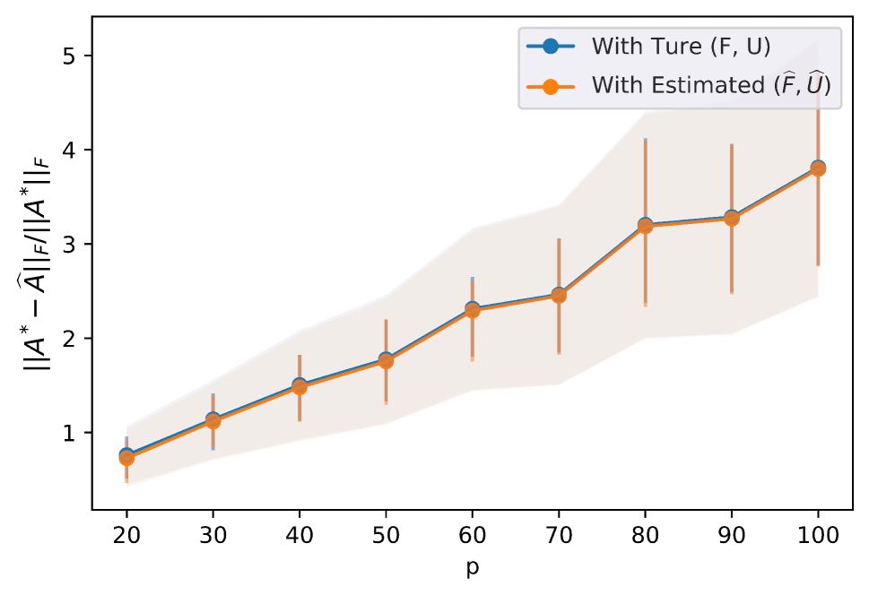
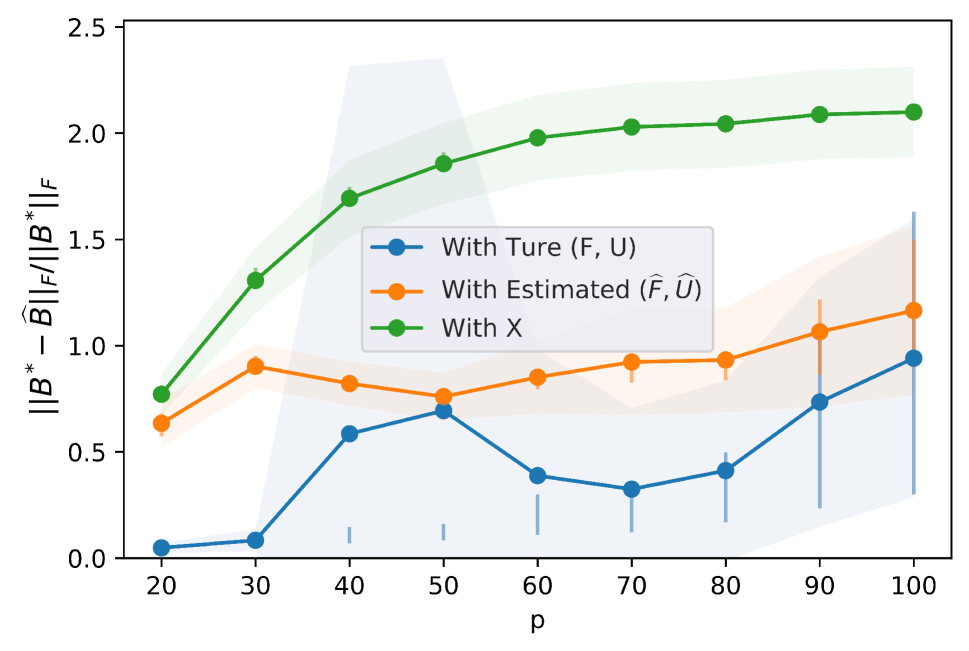
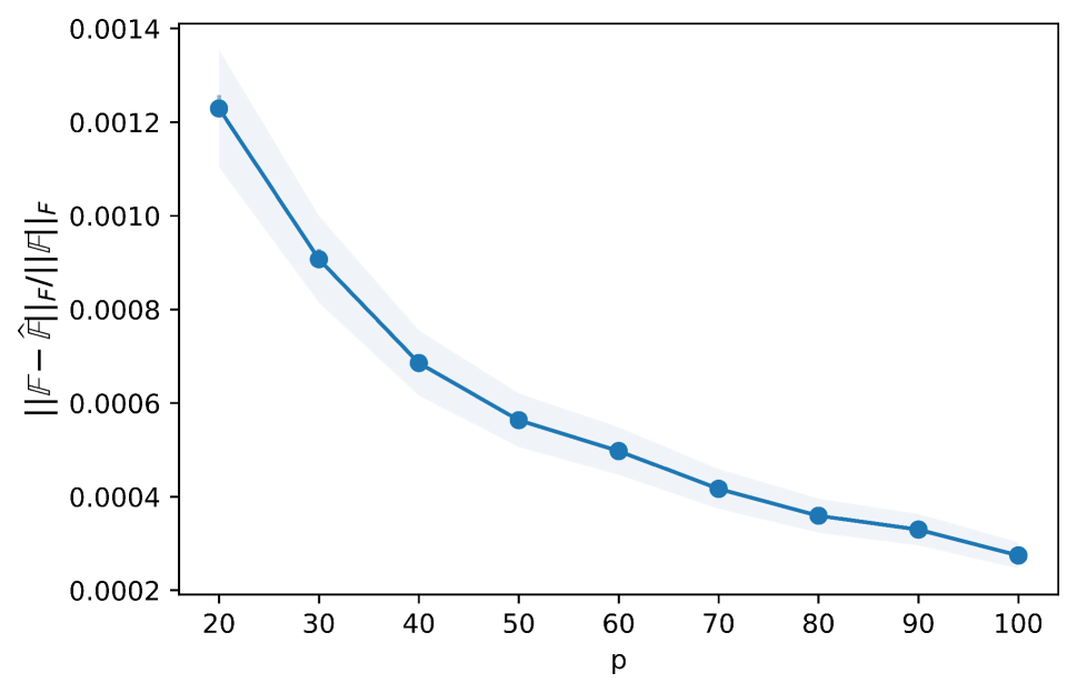
Figure 8: Fix $n=1000$, increase $p_{1}=p_{2}$ from $20$ to $100$. $\boldsymbol{A}^{*}$ is generated such that each elements are i.i.d from ${\cal N}(1000,1000^{2})$. The blue, orange, and green lines correspond to doing the regression with true $(\boldsymbol{F},\boldsymbol{U})$, estimated $(\widehat{\boldsymbol{F}},\widehat{\boldsymbol{U}})$, and $\boldsymbol{X}$, respectively. The experiments are repeated 100 times. The solid lines are the means, the shadows show the standard deviation, and the vertical lines present the quartiles.

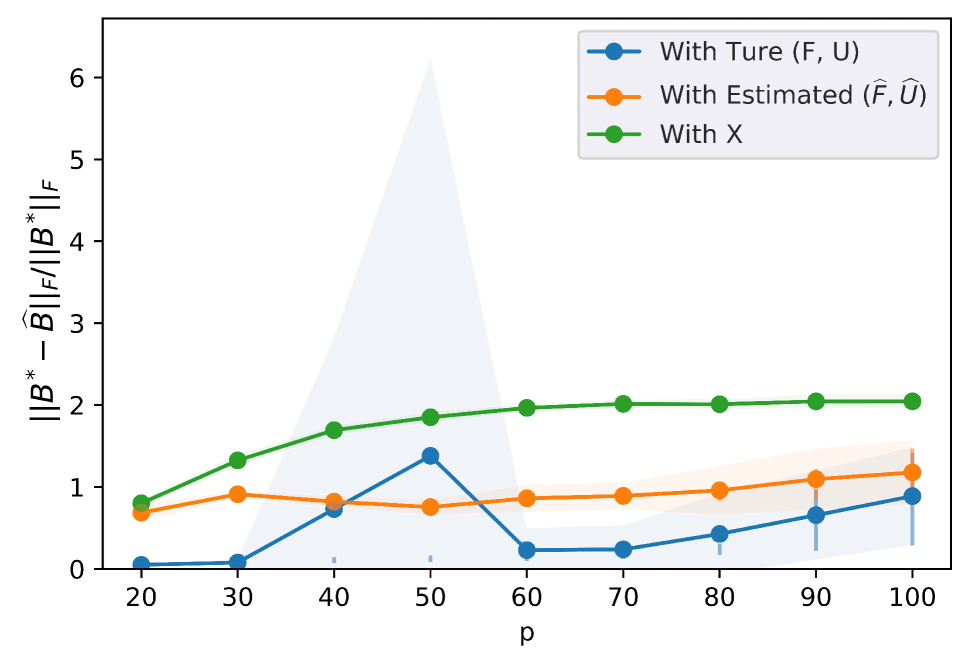
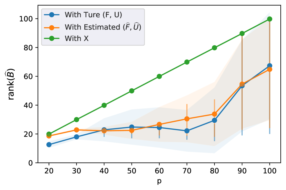
Figure 9: Fix $n=1000$, increase $p_{1}=p_{2}$ from $20$ to $100$. $\boldsymbol{A}^{*}$ is generated such that each elements are i.i.d from ${\cal N}(p_{1}p_{2},(p_{1}p_{2})^{2})$. The blue, orange, and green lines correspond to doing the regression with true $(\boldsymbol{F},\boldsymbol{U})$, estimated $(\widehat{\boldsymbol{F}},\widehat{\boldsymbol{U}})$, and $\boldsymbol{X}$, respectively. The experiments are repeated 100 times. The solid lines are the means, the shadows show the standard deviation, and the vertical lines present the quartiles.

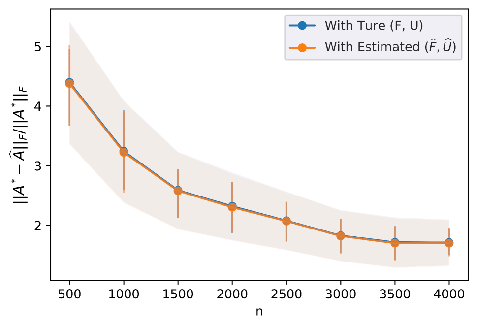
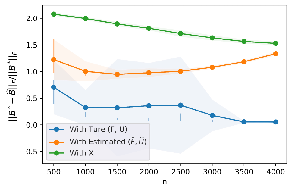
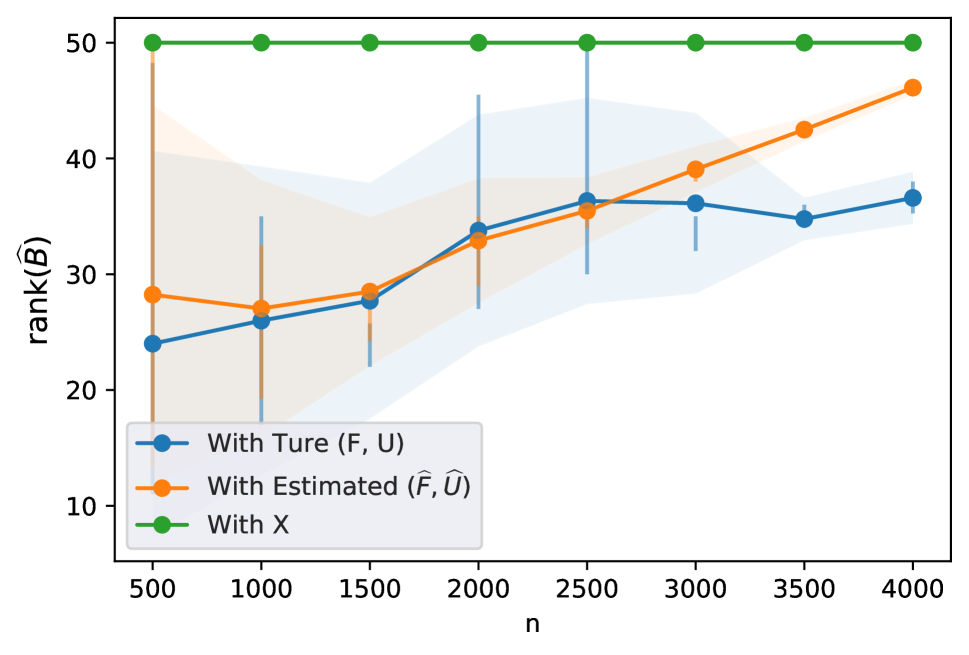
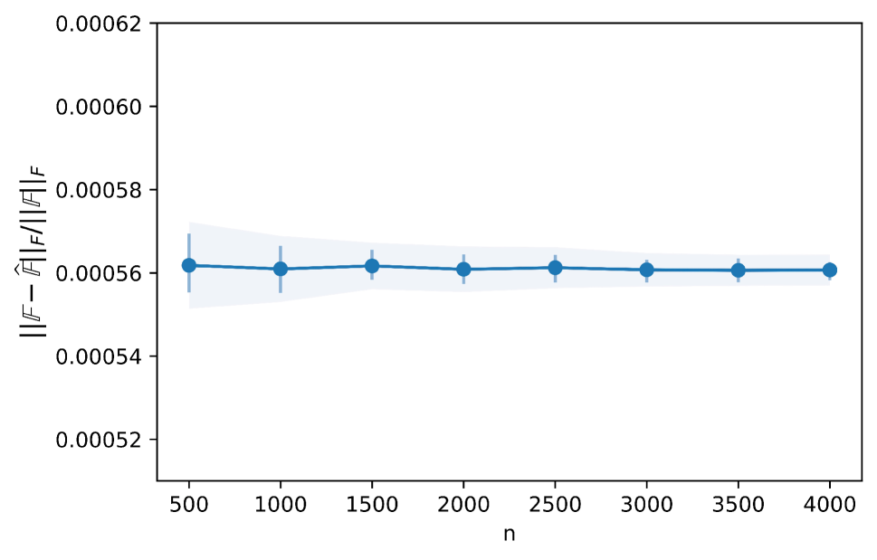
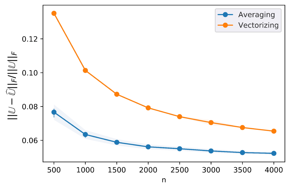
Figure 10: Fix $(p_{1},p_{2})=(70,50)$, increase $n$ from $500$ to $4000$. $\boldsymbol{A}^{*}$ is generated such that each elements are i.i.d from ${\cal N}(1000,1000^{2})$. The blue, orange, and green lines correspond to doing the regression with true $(\boldsymbol{F},\boldsymbol{U})$, estimated $(\widehat{\boldsymbol{F}},\widehat{\boldsymbol{U}})$, and $\boldsymbol{X}$, respectively. The experiments are repeated 100 times. The solid lines are the means, the shadows show the standard deviation, and the vertical lines present the quartiles.

I.2 FAMAR Matrix Loading Asymptotically Normality.

We present the full graph of the asymptotic normality check of the estimated loadings $\widehat{\boldsymbol{R}}$ and $\widehat{\boldsymbol{C}}$ according to Theorem 9 in Figure 11.

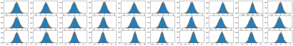
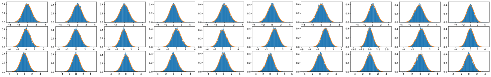
(a) Elements for $\sqrt{np_{2}k_{2}}\left(\widehat{\boldsymbol{R}}-\mathring{c}_{s}\mathring{\boldsymbol{R}^{*}}\right)^{\top}/\widehat{s}_{1}\in\mathbb{R}^{3\times 20}$

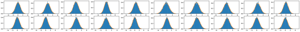
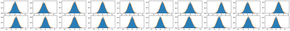
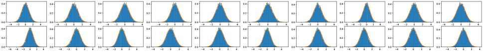
(b) Elements for $\sqrt{np_{1}k_{1}}\left(\widehat{\boldsymbol{C}}-\mathring{r}_{s}\mathring{\boldsymbol{C}^{*}}\right)^{\top}/\widehat{s}_{2}\in\mathbb{R}^{2\times 30}$

Figure 11: Elementwise normality check for the estimated loadings $\widehat{\boldsymbol{R}}$ and $\widehat{\boldsymbol{C}}$ according to Theorem 9. The blue histograms are empirical densities, and the orange lines are the standard Gaussian density functions.

References

- (1)
- Banerjee et al. (2005) Banerjee, A., Marcellino, M. & Masten, I. (2005), ‘Leading indicators for euro-area inflation and gdp growth’, Oxford Bulletin of Economics and Statistics 67, 785–813.
- Bertsekas et al. (1999) Bertsekas, D. P., Hager, W. & Mangasarian, O. (1999), ‘Nonlinear programming. athena scientific belmont’, Massachusets, USA .
- Cai et al. (2010) Cai, J.-F., Candès, E. J. & Shen, Z. (2010), ‘A singular value thresholding algorithm for matrix completion’, SIAM Journal on optimization 20(4), 1956–1982.
- Chen & Fan (2021) Chen, E. Y. & Fan, J. (2021), ‘Statistical inference for high-dimensional matrix-variate factor models’, Journal of the American Statistical Association pp. 1–18.
- Chen et al. (2023) Chen, E. Y., Fan, J. & Zhu, X. (2023), ‘Community network auto-regression for high-dimensional time series’, Journal of Econometrics 235(2), 1239–1256.
- Chen et al. (2019) Chen, E. Y., Tsay, R. S. & Chen, R. (2019), ‘Constrained factor models for high-dimensional matrix-variate time series’, Journal of the American Statistical Association .
- Chen et al. (2020) Chen, E. Y., Xia, D., Cai, C. & Fan, J. (2020), ‘Semiparametric tensor factor analysis by iteratively projected svd’, arXiv preprint arXiv:2007.02404 .
- Fan et al. (2019) Fan, J., Gong, W. & Zhu, Z. (2019), ‘Generalized high-dimensional trace regression via nuclear norm regularization’, Journal of econometrics 212(1), 177–202.
- Fan & Gu (2022) Fan, J. & Gu, Y. (2022), ‘Factor augmented sparse throughput deep relu neural networks for high dimensional regression’, arXiv preprint arXiv:2210.02002 .
- Fan, Ke & Wang (2020) Fan, J., Ke, Y. & Wang, K. (2020), ‘Factor-adjusted regularized model selection’, Journal of econometrics 216(1), 71–85.
- Fan, Li, Zhang & Zou (2020) Fan, J., Li, R., Zhang, C.-H. & Zou, H. (2020), Statistical foundations of data science, Chapman and Hall/CRC.
- Fan & Liao (2022) Fan, J. & Liao, Y. (2022), ‘Learning latent factors from diversified projections and its applications to over-estimated and weak factors’, Journal of the American Statistical Association 117(538), 909–924.
- Fan et al. (2013) Fan, J., Liao, Y. & Mincheva, M. (2013), ‘Large covariance estimation by thresholding principal orthogonal complements’, Journal of the Royal Statistical Society Series B: Statistical Methodology 75(4), 603–680.
- Fan et al. (2023) Fan, J., Lou, Z. & Yu, M. (2023), ‘Are latent factor regression and sparse regression adequate?’, Journal of the American Statistical Association (just-accepted), 1–77.
- Hastie et al. (2015) Hastie, T., Tibshirani, R. & Wainwright, M. (2015), ‘Statistical learning with sparsity’, Monographs on statistics and applied probability 143(143), 8.
- Ji & Ye (2009) Ji, S. & Ye, J. (2009), An accelerated gradient method for trace norm minimization, in ‘Proceedings of the 26th annual international conference on machine learning’, pp. 457–464.
- Kopoin et al. (2013) Kopoin, A., Moran, K. & Paré, J.-P. (2013), ‘Forecasting regional gdp with factor models: How useful are national and international data?’, Economics Letters 121(2), 267–270.
- Liu & Chen (2022) Liu, X. & Chen, E. Y. (2022), ‘Identification and estimation of threshold matrix-variate factor models’, Scandinavian Journal of Statistics 49(3), 1383–1417.
- Negahban & Wainwright (2011) Negahban, S. & Wainwright, M. J. (2011), ‘Estimation of (near) low-rank matrices with noise and high-dimensional scaling’.
- Nesterov (2013) Nesterov, Y. (2013), ‘Gradient methods for minimizing composite functions’, Mathematical programming 140(1), 125–161.
- Nogay & Adeli (2020) Nogay, H. S. & Adeli, H. (2020), ‘Machine learning (ml) for the diagnosis of autism spectrum disorder (asd) using brain imaging’, Reviews in the Neurosciences 31(8), 825–841.
- Obozinski et al. (2011) Obozinski, G., Wainwright, M. J. & Jordan, M. I. (2011), ‘Support union recovery in high-dimensional multivariate regression’.
- Recht et al. (2010) Recht, B., Fazel, M. & Parrilo, P. A. (2010), ‘Guaranteed minimum-rank solutions of linear matrix equations via nuclear norm minimization’, SIAM review 52(3), 471–501.
- Simon et al. (2013) Simon, N., Friedman, J., Hastie, T. & Tibshirani, R. (2013), ‘A sparse-group lasso’, Journal of computational and graphical statistics 22(2), 231–245.
- Wainwright (2019) Wainwright, M. J. (2019), High-dimensional statistics: A non-asymptotic viewpoint, Vol. 48, Cambridge University Press.
- Wang et al. (2017) Wang, X., Zhu, H. & Initiative, A. D. N. (2017), ‘Generalized scalar-on-image regression models via total variation’, Journal of the American Statistical Association 112(519), 1156–1168.
- Yang & Zou (2015) Yang, Y. & Zou, H. (2015), ‘A fast unified algorithm for solving group-lasso penalize learning problems’, Statistics and Computing 25, 1129–1141.
- Yu et al. (2015) Yu, D., Won, J.-H., Lee, T., Lim, J. & Yoon, S. (2015), ‘High-dimensional fused lasso regression using majorization–minimization and parallel processing’, Journal of Computational and Graphical Statistics 24(1), 121–153.
- Yu et al. (2022) Yu, L., He, Y., Kong, X. & Zhang, X. (2022), ‘Projected estimation for large-dimensional matrix factor models’, Journal of Econometrics 229(1), 201–217.
- Yuan & Lin (2006) Yuan, M. & Lin, Y. (2006), ‘Model selection and estimation in regression with grouped variables’, Journal of the Royal Statistical Society Series B: Statistical Methodology 68(1), 49–67.
- Zhou & Li (2014) Zhou, H. & Li, L. (2014), ‘Regularized matrix regression’, Journal of the Royal Statistical Society: Series B (Statistical Methodology) 76(2), 463–483.
- Zhou et al. (2021) Zhou, Y., Xue, L., Shi, Z., Wu, L. & Fan, J. (2021), ‘Measuring housing activeness from multi-source big data and machine learning’, Available at SSRN 3940180 .
SUPPLEMENTARY MATERIAL of