Probabilistic Verification of Neural Networks using Branch and Bound

Abstract

Probabilistic verification of neural networks is concerned with formally analysing the output distribution of a neural network under a probability distribution of the inputs. Examples of probabilistic verification include verifying the demographic parity fairness notion or quantifying the safety of a neural network. We present a new algorithm for the probabilistic verification of neural networks based on an algorithm for computing and iteratively refining lower and upper bounds on probabilities over the outputs of a neural network. By applying state-of-the-art bound propagation and branch and bound techniques from non-probabilistic neural network verification, our algorithm significantly outpaces existing probabilistic verification algorithms, reducing solving times for various benchmarks from the literature from tens of minutes to tens of seconds. Furthermore, our algorithm compares favourably even to dedicated algorithms for restricted subsets of probabilistic verification. We complement our empirical evaluation with a theoretical analysis, proving that our algorithm is sound and, under mildly restrictive conditions, also complete when using a suitable set of heuristics.

1 Introduction

As deep learning spreads through society, it becomes increasingly important to ensure the reliability of artificial neural networks, including aspects of fairness and safety. However, manually introspecting neural networks is infeasible due to their opaque nature, and empirical assessments of neural networks are challenged by neural networks being fragile with respect to various types of input perturbations [SzegedyZarembaSutskeverEtAl2014, HendrycksZhaoBasartEtAl2021, HendrycksDietterich2019, HosseiniXiaoPoovendran2017, CarliniWagner2018, EbrahimiRaoLowdEtAl2018, BibiAlfadlyGhanem2018]. In contrast, neural network verification analyses neural networks with mathematical rigour, facilitating the faithful auditing of neural networks.

In this paper, we consider probabilistic verification of neural networks, which is concerned with proving statements about the output distribution of a neural network. An example of probabilistic verification is proving that a neural network $\mathsf{net}$ making a binary decision affecting a person (for example, hire/do not hire, credit approved/denied) satisfies the demographic parity fairness notion [BarocasHardtNarayanan2023] under a probability distribution $\mathbb{P}_{\mathbf{x}}$ of the network inputs $\mathbf{x}$ representing the person

$$\frac{\mathbb{P}_{\mathbf{x}}{\mathchoice{\left[\mathsf{net}(\mathbf{x})=\texttt{yes}\mid\mathbf{x}\ \text{is disadvantaged}\right]}{[\mathsf{net}(\mathbf{x})=\texttt{yes}\mid\mathbf{x}\ \text{is disadvantaged}]}{\left[\mathsf{net}(\mathbf{x})=\texttt{yes}\mid\mathbf{x}\ \text{is disadvantaged}\right]}{\left[\mathsf{net}(\mathbf{x})=\texttt{yes}\mid\mathbf{x}\ \text{is disadvantaged}\right]}}}{\mathbb{P}_{\mathbf{x}}{\mathchoice{\left[\mathsf{net}(\mathbf{x})=\texttt{yes}\mid\mathbf{x}\ \text{is advantaged}\right]}{[\mathsf{net}(\mathbf{x})=\texttt{yes}\mid\mathbf{x}\ \text{is advantaged}]}{\left[\mathsf{net}(\mathbf{x})=\texttt{yes}\mid\mathbf{x}\ \text{is advantaged}\right]}{\left[\mathsf{net}(\mathbf{x})=\texttt{yes}\mid\mathbf{x}\ \text{is advantaged}\right]}}}\geq\gamma,$$ (1)

where $\gamma\in[0,1]$ with $\gamma=0.8$ being a common choice [FeldmanFriedlerMoellerEtAl2015]. A closely related problem to probabilistic verification is computing bounds on probabilities over a neural network. An example of this is quantifying the safety of a neural network by bounding

$$\mathbb{P}_{\mathbf{x}}{\mathchoice{\left[\mathsf{net}(\mathbf{x})\ \text{is unsafe}\right]}{[\mathsf{net}(\mathbf{x})\ \text{is unsafe}]}{\left[\mathsf{net}(\mathbf{x})\ \text{is unsafe}\right]}{\left[\mathsf{net}(\mathbf{x})\ \text{is unsafe}\right]}}.$$ (2)

In this paper, we introduce a novel algorithm for computing bounds on probabilities such as Equation 2 using a branch and bound framework [LandDoig2010, MorrisonJacobsonSauppeEtAl2016]. These bounds then allow us to verify probabilistic statements like Equation 1 using ideas from the probabilistic verification algorithm FairSquare [AlbarghouthiDAntoniDrewsEtAl2017].

More concretely, we recombine neural network verification using branch and bound [BunelLuTurkaslanEtAl2020], linear relaxations of neural networks [ZhangWengChenEtAl2018, SinghGehrPueschelEtAl2019], and massively parallel branch and bound [XuZhangWangEtAl2021] with ideas from FairSquare [AlbarghouthiDAntoniDrewsEtAl2017] for probabilistic neural network verification, to obtain the Probabilistic Verification (PV) algorithm, a fast and generally applicable probabilistic verification algorithm for neural networks. Our theoretical analysis of PV shows that PV is sound and, under mildly restrictive conditions, complete when using suitable branching and splitting heuristics.

Our experimental evaluation reveals that PV significantly outpaces the probabilistic verification algorithms FairSquare [AlbarghouthiDAntoniDrewsEtAl2017] and SpaceScanner [ConverseFilieriGopinathEtAl2020]. In particular, we solve benchmark instances that FairSquare can not solve within 15 minutes in less than 10 seconds and solve the ACAS Xu [KatzBarrettDillEtAl2017] probabilistic robustness case study of [ConverseFilieriGopinathEtAl2020] in a mean runtime of 18 seconds, compared to 33 minutes for SpaceScanner.

Applying PV to #DNN verification [MarzariCorsiCicaleseEtAl2023], a subset of probabilistic verification, reveals that PV also compares favourably to the ProVe_SLR algorithm [MarzariRoncolatoFarinelli2023] specialised to #DNN verification and even the $\varepsilon$-ProVe algorithm [MarzariCorsiMarchesiniEtAl2024] that relaxes #DNN verification to computing a confidence interval on the solution. In contrast to $\varepsilon$-ProVe and similar approaches [WengChenNguyenEtAl2019, BastaniZhangSolarLezama2019, BalutaShenShindeEtAl2019], PV computes lower and upper bounds on probabilities like Equation 2 that are guaranteed to hold with absolute certainty. Such bounds are preferable to confidence intervals in high-risk machine-learning applications.

To test the limits of PV and fuel further research in probabilistic verification, we introduce a significantly more challenging probabilistic verification benchmark: MiniACSIncome is a benchmark based on the ACSIncome dataset [DingHardtMillerEtAl2021] and is concerned with verifying the demographic parity of neural networks for datasets of increasing input dimensionality. In summary, our contributions are

• the PV algorithm for the probabilistic verification of neural networks,

• a theoretical analysis of PV,

• a thorough experimental comparison of PV with existing probabilistic verifiers for neural networks and tools dedicated to restricted subsets of probabilistic verification, and

• MiniACSIncome: a new, challenging probabilistic verification benchmark.

2 Related Work

Non-probabilistic neural network verification is concerned with proving that the outputs of a neural network satisfy some condition for all inputs in an input set. Approaches for non-probablistic neural network verification include Satisfiability Modulo Theories (SMT) solving [KatzBarrettDillEtAl2017, WuIsacZeljicEtAl2024, DuongLiNguyenEtAl2023], Mixed Integer Linear Programming (MILP) [TjengXiaoTedrake2019, ChengNuehrenbergRuess2017, AndersonHuchetteMaEtAl2020], and Reachability Analysis [BakTranHobbsEtAl2020, TranBakXiangEtAl2020, TranYangLopezEtAl2020]. Many of these approaches can be understood as branch and bound algorithms [BunelLuTurkaslanEtAl2020]. Branch and bound [LandDoig2010, MorrisonJacobsonSauppeEtAl2016] also powers the $\alpha,\!\beta$-CROWN [ZhangWangXuEtAl2022], MN-BaB [FerrariMuellerJovanovicEtAl2022] and VeriNet [HenriksenLomuscio2021] verifiers that lead the table in recent international neural network verifier competitions [MuellerBrixBakEtAl2022, BrixBakLiuEtAl2023].

A critical component of a branch and bound verification algorithm is computing bounds on the output of a neural network. Approaches for bounding neural network outputs include interval arithmetic [PulinaTacchella2010, ChengNuehrenbergRuess2017], dual approaches [WongKolter2018], linear bound propagation techniques [WengZhangChenEtAl2018, SinghGehrPueschelEtAl2019, ZhangWengChenEtAl2018], multi-neuron linear relaxations [MuellerMakarchukSinghEtAl2022], and further optimisation-based approaches [XuZhangWangEtAl2021, PalmaBehlBunelEtAl2021, BunelPalmaDesmaisonEtAl2020].

Probabilistic verification algorithms can be divided into sound algorithms that provide valid proofs and probably sound algorithms that provide valid proofs with a certain predefined probability. FairSquare [AlbarghouthiDAntoniDrewsEtAl2017] is a fairness verification algorithm, a subset of probabilistic verification that studies problems such as Equation 1. FairSquare uses SMT solving for splitting the input space into disjoint hyperrectangles, integrating over which yields bounds on a target probability. [ConverseFilieriGopinathEtAl2020] (SpaceScanner) and [BorcaTasciucGuoBakEtAl2023] divide the input space into disjoint polytopes using concolic execution and reachable set verification, respectively, to perform probabilistic verification. [MorettinPasseriniSebastiani2024] use weighted model integration [BellePasseriniBroeck2015] to obtain a general probabilistic verification algorithm but neither provide code nor report runtimes. A restricted subset of probabilistic verification is #DNN verification [MarzariCorsiCicaleseEtAl2023], corresponding to probabilistic verification under uniformly distributed inputs. The #DNN verifier ProVe_SLR [MarzariRoncolatoFarinelli2023] uses a similar massively parallel branch and bound approach as our algorithm but does not perform general probabilistic verification.

Probably sound verification algorithms [BastaniZhangSolarLezama2019, BalutaShenShindeEtAl2019, MarzariCorsiCicaleseEtAl2023, MarzariCorsiMarchesiniEtAl2024] obtain efficiency at the cost of potentially unsound results. $\varepsilon$-ProVe [MarzariCorsiMarchesiniEtAl2024] is a probably sound #DNN verification algorithm. [ConverseFilieriGopinathEtAl2020, BastaniZhangSolarLezama2019, MarzariRoncolatoFarinelli2023] compare sound and probably sound approaches for fairness verification, general probabilistic verification, and #DNN verification, respectively. We study sound probabilistic verification since certainly sound results are preferable in critical applications, such as education [EuropeanParliament2023], medical applications, or autonomous driving and flight.

Besides probabilistic fairness notions, such as demographic parity [BarocasHardtNarayanan2023], several approaches [RuossBalunovicFischerEtAl2020, UrbanChristakisWuestholzEtAl2020, BiswasRajan2023, MohammadiSivaramanFarnadi2023] verify dependency fairness [GalhotraBrunMeliou2017, UrbanChristakisWuestholzEtAl2020], an individual fairness notion [DworkHardtPitassiEtAl2012] that states that persons that only differ by their protected attribute (for example, gender or race) need to be assigned to the same class. However, dependency fairness can be satisfied trivially by withholding the protected attribute from the classifier. Since withholding the protected attribute is insufficient [PedreschiRuggieriTurini2008] or even harmful [KusnerLoftusRussellEtAl2017] for fairness, dependency fairness is an insufficient fairness notion.

3 Preliminaries and Problem Statement

Throughout this paper, we are concerned with computing (provable) lower and upper bounds on various functions.

Definition 1 (Bounds).

For $f:\mathbb{R}^{n}\to\mathbb{R}^{m}$, we call $\ell,u\in\mathbb{R}^{m}$ a lower, respectively, upper bound on $f$ for $\mathcal{X}^{\prime}\subseteq\mathbb{R}^{n}$ if $\ell\leq f(\mathbf{x})\leq u,\forall\mathbf{x}\in\mathcal{X}^{\prime}$.

Neural Networks.

In particular, we are concerned with computing bounds on functions involving neural networks $\mathsf{net}:\mathcal{X}\to\mathbb{R}^{m}$, where $\mathcal{X}\subset\mathbb{R}^{n}$ is the input space of the neural network. A neural network is a composition of linear functions and a predefined set of non-linear functions, such as ReLU, Tanh, and max pooling. We refrain from further defining neural networks but refer the interested reader to the auto_LiRPA library [XuShiZhangEtAl2020b] that practically defines the class of neural networks to which our algorithm can be applied. For the scope of this paper, we only consider fully-connected feed-forward neural networks.

Throughout this paper, we assume that the input space $\mathcal{X}$ is a bounded hyperrectangle. Bounded input spaces are common in machine learning. Examples include the space of normalised images ${[0,1]}^{n}$ in computer vision and tabular input spaces of practically bounded variables, such as age, working hours per week, income, etc.

Notation and Terminology.

We use bold letters ($\mathbf{x}$, $\mathbf{y}$) for vectors and calligraphic letters ($\mathcal{X}$) for sets. Let $\underline{\mathbf{x}},\overline{\mathbf{x}}\in\mathbb{R}^{n}$ with $\underline{\mathbf{x}}\leq\overline{\mathbf{x}}$. We use $[\underline{\mathbf{x}},\overline{\mathbf{x}}]=\{\mathbf{x}\in\mathbb{R}^{n}\mid\underline{\mathbf{x}}\leq\mathbf{x}\leq\overline{\mathbf{x}}\}$ to denote the hyperrectangle with the minimal element $\underline{\mathbf{x}}$ and the maximal element $\overline{\mathbf{x}}$. When we speak of bounds on a certain quantity in this paper, we refer to a pair of a lower and an upper bound. Throughout this paper, $\ell,\mathdcal{k}$ denote lower bounds, and $u$ denotes an upper bound. When convenient, we also use $\underline{\mathbf{y}}\leq\mathbf{y}\leq\overline{\mathbf{y}}$ to denote bounds, especially on vectors. We assume that all random objects are defined on the same abstract probability space $(\Omega,\mathcal{F},\mathbb{P})$ and that all continuous random variables admit a probability density function.

3.1 Probabilistic Verification of Neural Networks

Let $\mathcal{X}\subset\mathbb{R}^{n}$ be a bounded hyperrectangle and let $v\in\mathbb{N}$. In this paper, we are concerned with proving or disproving whether $\mathsf{net}:\mathcal{X}\to\mathbb{R}^{m}$ is feasible for the probabilistic verification problem

$$P:\left\{\,\begin{array}[]{l}f_{\mathrm{Sat}}(p_{1},\ldots,p_{v})\geq 0,\\ p_{i}=\mathbb{P}_{\mathbf{x}^{(i)}}{\mathchoice{\left[g_{\mathrm{Sat}}^{(i)}(\mathbf{x}^{(i)},\mathsf{net}(\mathbf{x}^{(i)}))\geq 0\right]}{[g_{\mathrm{Sat}}^{(i)}(\mathbf{x}^{(i)},\mathsf{net}(\mathbf{x}^{(i)}))\geq 0]}{\left[g_{\mathrm{Sat}}^{(i)}(\mathbf{x}^{(i)},\mathsf{net}(\mathbf{x}^{(i)}))\geq 0\right]}{\left[g_{\mathrm{Sat}}^{(i)}(\mathbf{x}^{(i)},\mathsf{net}(\mathbf{x}^{(i)}))\geq 0\right]}}\quad\forall i\in\{1,\ldots,v\},\end{array}\right.$$ (3)

where $\mathbf{x}^{(i)}$, $i\in\{1,\ldots,v\}$, is a $\mathcal{X}$-valued random variable with distribution $\mathbb{P}_{\mathbf{x}^{(i)}}$ and $f_{\mathrm{Sat}}:\mathbb{R}^{v}\to\mathbb{R}$, $g_{\mathrm{Sat}}^{(i)}:\mathbb{R}^{n}\times\mathbb{R}^{m}\to\mathbb{R}$, $i\in\{1,\ldots,v\}$ are satisfaction functions. We only consider satisfaction functions that are compositions of linear functions, multiplication, division, and monotone functions, such as ReLU, Sigmoid, $\min$ and $\max$. Throughout this paper, we assume all probabilistic verification problems to be well-defined.

Example 1.

We express the demographic parity fairness notion from Equation 1 as a probabilistic verification problem. Let $\mathcal{X}\subset\mathbb{R}^{n}$ be an input space containing a categorical protected attribute, such as gender, race, or disability status that is one-hot encoded at the indices $A\subset\{1,\ldots,n\}$. We assume a single historically advantaged category encoded at the index $a\in A$. Consider a neural network $\mathsf{net}:\mathbb{R}^{n}\to\mathbb{R}^{2}$ that acts as a binary classifier making a decision affecting a person, such as hiring or credit approval. The neural network produces a score for each class and assigns the class with the higher score to an input. We express Equation 1 as a probabilistic verification problem, that is,

$$\frac{\mathbb{P}_{\mathbf{x}}{\mathchoice{\left[\mathsf{net}(\mathbf{x})=\texttt{yes}\mid\mathbf{x}\ \text{is disadvantaged}\right]}{[\mathsf{net}(\mathbf{x})=\texttt{yes}\mid\mathbf{x}\ \text{is disadvantaged}]}{\left[\mathsf{net}(\mathbf{x})=\texttt{yes}\mid\mathbf{x}\ \text{is disadvantaged}\right]}{\left[\mathsf{net}(\mathbf{x})=\texttt{yes}\mid\mathbf{x}\ \text{is disadvantaged}\right]}}}{\mathbb{P}_{\mathbf{x}}{\mathchoice{\left[\mathsf{net}(\mathbf{x})=\texttt{yes}\mid\mathbf{x}\ \text{is advantaged}\right]}{[\mathsf{net}(\mathbf{x})=\texttt{yes}\mid\mathbf{x}\ \text{is advantaged}]}{\left[\mathsf{net}(\mathbf{x})=\texttt{yes}\mid\mathbf{x}\ \text{is advantaged}\right]}{\left[\mathsf{net}(\mathbf{x})=\texttt{yes}\mid\mathbf{x}\ \text{is advantaged}\right]}}}\geq\gamma\quad\Longleftrightarrow\quad\mathsf{net}\ \text{is feasible in \lx@cref{creftype~refnum}{eqn:pvp}},$$

where, $f_{\mathrm{Sat}}(p_{1},p_{2},p_{3},p_{4})=(p_{1}p_{4})/(p_{2}p_{3})-\gamma$, $g_{\mathrm{Sat}}^{(1)}(\mathbf{x},\mathsf{net}(\mathbf{x}))=\min({\mathsf{net}(\mathbf{x})}_{1}-{\mathsf{net}(\mathbf{x})}_{2},-\mathbf{x}_{a})$, $g_{\mathrm{Sat}}^{(2)}(\mathbf{x},\mathsf{net}(\mathbf{x}))=-\mathbf{x}_{a}$, $g_{\mathrm{Sat}}^{(3)}(\mathbf{x},\mathsf{net}(\mathbf{x}))=\min({\mathsf{net}(\mathbf{x})}_{1}-{\mathsf{net}(\mathbf{x})}_{2},\mathbf{x}_{a}-1)$, and $g_{\mathrm{Sat}}^{(4)}(\mathbf{x},\mathsf{net}(\mathbf{x}))=\mathbf{x}_{a}-1$. LABEL:sec:spec-extended-example contains a detailed derivation of this equivalence.

If all inputs $\mathbf{x}^{(i)}$ are uniformly distributed, probabilistic verification corresponds to #DNN verification [MarzariCorsiCicaleseEtAl2023]. As [MarzariCorsiCicaleseEtAl2023] prove, #DNN verification is #P complete, implying that probabilistic verification is #P hard. Since #P is at least as hard as NP, we can not expect to obtain efficient algorithms, but which probabilistic verification problems are practically solvable remains undetermined.

3.2 Non-Probabilistic Neural Network Verification

The goal of non-probabilistic neural network verification is to prove or disprove whether a neural network $\mathsf{net}:\mathcal{X}\to\mathbb{R}^{m}$ is feasible for

$$V:\;g_{\mathrm{Sat}}(\mathbf{x},\mathsf{net}(\mathbf{x}))\geq 0{}\quad\forall\mathbf{x}\in\mathcal{X}^{\prime},$$ (4)

where $\mathcal{X}^{\prime}\subseteq\mathcal{X}$ is a hyperrectangle, and $g_{\mathrm{Sat}}:\mathbb{R}^{n}\times\mathbb{R}^{m}\to\mathbb{R}$ is a satisfaction function that indicates whether the output of $\mathsf{net}$ is desirable ($g_{\mathrm{Sat}}(\cdot,\mathsf{net}(\cdot))\geq 0$) or undesirable ($g_{\mathrm{Sat}}(\cdot,\mathsf{net}(\cdot))<0$). In (non-probabilistic) neural network verification, $g_{\mathrm{Sat}}$ can generally be considered a part of $\mathsf{net}$ [BunelLuTurkaslanEtAl2020, XuShiZhangEtAl2020b]. Neural network verifiers are algorithms for proving or disproving Equation 4. Two desirable properties of neural network verifiers are soundness and completeness.

Definition 2 (Soundness and Completeness).

A verification algorithm is sound if it only produces genuine counterexamples and valid proofs for Equation 4. It is complete if it produces a counterexample or proof for Equation 4 for any neural network in a finite amount of time.

Analogous notions of soundness and completeness also apply to probabilistic verifiers. Generally unsound but probably sound probabilistic verification approaches are discussed in Section 2. We introduce incomplete and complete neural network verification through two examples: interval arithmetic and branch and bound.

3.2.1 Interval Arithmetic

Interval arithmetic [MooreKearfottCloud2009] is a bound propagation technique that derives bounds on the output of a neural network from bounds on the network input. Assume $\underline{\mathbf{x}missing}\leq\mathbf{x}\leq\overline{\mathbf{x}}$ are bounds on the network input $\mathbf{x}$ and we apply interval arithmetic to compute $\ell\leq g_{\mathrm{Sat}}(\mathbf{x},\mathsf{net}(\mathbf{x}))\leq u$, $\forall\mathbf{x}\in[\underline{\mathbf{x}missing},\overline{\mathbf{x}}]$. If the lower bound is large enough or the upper bound small enough, we can prove or disprove Equation 4 using

$$\ell\geq 0\Longrightarrow g_{\mathrm{Sat}}(\mathbf{x},\mathsf{net}(\mathbf{x}))\geq 0,\qquad\text{respectively,}\qquad u<0\Longrightarrow g_{\mathrm{Sat}}(\mathbf{x},\mathsf{net}(\mathbf{x}))<0.$$

However, if the bounds are inconclusive, that is $\ell<0\leq u$, we can neither prove nor disprove Equation 4. The possibility of inconclusive results makes interval arithmetic an incomplete technique for neural network verification. In particular, interval arithmetic is relatively imprecise, meaning that bounds derived using interval arithmetic are frequently inconclusive [GehrMirmanDrachslerCohenEtAl2018]. More precise approaches include DeepPoly [SinghGehrPueschelEtAl2019] and CROWN [ZhangWengChenEtAl2018] that follow the same overall scheme but propagate linear bounds through a neural network. We primarily employ interval arithmetic to compute bounds on the $f_{\mathrm{Sat}}$ function in Equation 3 given bounds on $p_{1},\ldots,p_{v}$.

Let $f:\mathbb{R}^{n}\to\mathbb{R}$ be a function that we want to bound for inputs $\mathbf{x}\in[\underline{\mathbf{x}missing},\overline{\mathbf{x}}]$. Interval arithmetic and other bound propagation techniques rely on $f=f^{(K)}\circ\cdots\circ f^{(1)}$ being a composition of more fundamental functions $f^{(k)}:\mathbb{R}^{n_{k}}\to\mathbb{R}^{n_{k+1}}$ for which we can already compute $\ell^{(k)}\leq f^{(k)}(\mathbf{z})\leq u^{(k)}$ given $\underline{\mathbf{z}}\leq\mathbf{z}\leq\overline{\mathbf{z}}$. Examples of such functions include monotone non-decreasing functions, for which $f^{(k)}(\underline{\mathbf{z}})\leq f^{(k)}(\mathbf{z})\leq f^{(k)}(\overline{\mathbf{z}})$, or monotone non-increasing functions, for which $f^{(k)}(\overline{\mathbf{z}})\leq f^{(k)}(\mathbf{z})\leq f^{(k)}(\underline{\mathbf{z}})$. These two bounding rules already allow us to bound addition, subtraction, $\min$, $\max$, and many popular neural network activation functions like ReLU, Sigmoid, and Tanh. LABEL:sec:interval-arithmetic-extra contains bounding rules for linear functions, multiplication, and division. Algorithm 1 describes how interval arithmetic computes bounds on $f$ using the bounding rules for $f^{(K)}\ldots,f^{(1)}$.

Input: Function $f=f^{(K)}\circ\ldots\circ f^{(1)}$, Input Bounds $\underline{\mathbf{x}missing},\overline{\mathbf{x}}$

1 $\underline{\mathbf{z}}^{(0)}\leftarrow\underline{\mathbf{x}missing}$, $\overline{\mathbf{z}}^{(0)}\leftarrow\overline{\mathbf{x}}$

2 for $k\in\{1,\ldots,K\}$ do $(\underline{\mathbf{z}}^{(k)},\overline{\mathbf{z}}^{(k)})\leftarrow\textsf{BoundingRule}(f^{(k)},\underline{\mathbf{z}}^{(k-1)},\overline{\mathbf{z}}^{(k-1)})$

3 return $\underline{\mathbf{z}}^{(K)},\overline{\mathbf{z}}^{(K)}$

Algorithm 1 Interval Arithmetic

3.2.2 Branch and Bound

Irrespective of their relative precision, bound propagation approaches such as interval arithmetic, DeepPoly [SinghGehrPueschelEtAl2019], and CROWN [ZhangWengChenEtAl2018] are incomplete according to 2. To obtain a complete verifier, bound propagation can be combined with branching to gain completeness. This algorithmic framework is called branch and bound [LandDoig2010, MorrisonJacobsonSauppeEtAl2016, BunelLuTurkaslanEtAl2020]. In branch and bound, when the computed bounds are inconclusive ($\ell<0\leq u$), the search space is split (branching). The idea is that splitting improves the precision of the bounds for each part of the split (each branch).

Algorithm 2 contains an abstract branch and bound algorithm for neural network verification. This algorithm has three subprocedures that we need to instantiate for running Algorithm 2: Select, ComputeBounds, and Split. One instantiation that yields a complete algorithm is selecting branches in a FIFO order, computing bounds using interval arithmetic and splitting the search space by bisecting the input space [WangPeiWhitehouseEtAl2018b]. [XuZhangWangEtAl2021] present an improved complete branch and bound algorithm that selects branches in batches to utilise massively parallel hardware such as GPUs, computes bounds using a combined bound propagation and optimisation procedure, and splits the search space by splitting on hidden ReLU nodes in the network [WangPeiWhitehouseEtAl2018]. We refer to [ZhangWangXuEtAl2022] for a state-of-the-art neural network verifier [MuellerBrixBakEtAl2022, BrixBakLiuEtAl2023] based on branch and bound. In the next section, we introduce a branch and bound algorithm for the probabilistic verification of neural networks.

Input: Verification Problem $g_{\mathrm{Sat}}(\mathbf{x},\mathsf{net}(\mathbf{x}))\geq 0,\forall\mathbf{x}\in\mathcal{X}^{\prime}$ where $\mathcal{X}^{\prime}=[\underline{\mathbf{x}missing},\overline{\mathbf{x}}]$

1 $\mathrm{branches}\leftarrow\{\mathcal{X}^{\prime}\}$

2 while $\mathrm{branches}\neq\emptyset$ do

      $[\underline{\mathbf{x}}^{\prime},\overline{\mathbf{x}}^{\prime}]\leftarrow\textsf{Select}(\mathrm{branches})$

        (Select one branch)

       $(\underline{y},\overline{y})\leftarrow\textsf{ComputeBounds}(g_{\mathrm{Sat}}(\cdot,\mathsf{net}(\cdot)),\underline{\mathbf{x}missing},\overline{\mathbf{x}})$

        (E.g. interval arithmetic)

3       if $\overline{y}<0$ then return Violated

4        (Every $\mathbf{x}\in[\underline{\mathbf{x}}^{\prime},\overline{\mathbf{x}}^{\prime}]$ is a counterexample) else if $\underline{y}\geq 0$ then $\mathrm{branches}\leftarrow(\mathrm{branches}\setminus\{[\underline{\mathbf{x}}^{\prime},\overline{\mathbf{x}}^{\prime}]\})$

5        (Prune branch) else

            $\mathrm{new}\leftarrow\textsf{Split}([\underline{\mathbf{x}}^{\prime},\overline{\mathbf{x}}^{\prime}])$

              (E.g. by bisection)

6             $\mathrm{branches}\leftarrow(\mathrm{branches}\setminus\{[\underline{\mathbf{x}}^{\prime},\overline{\mathbf{x}}^{\prime}]\})\cup\mathrm{new}$

7            

8      

return Satisfied

  (All branches pruned)

Algorithm 2 Branch and Bound for Non-Probabilistic Neural Network Verification

4 Algorithm

This section introduces Probabilistic Verification (PV), our algorithm for probabilistic verification of neural networks as defined in Equation 3. For conciseness, we use $p_{i}$ for $i\in\{1,\ldots,v\}$ as in Equation 3 and drop the index and superscripts ⁽ⁱ⁾ whenever we only consider a single probability $p$. PV uses the same overall approach as FairSquare [AlbarghouthiDAntoniDrewsEtAl2017]: Iteratively refine bounds on each $p_{i}$ until interval arithmetic allows us to prove or disprove $f_{\mathrm{Sat}}(p_{1},\ldots,p_{v})\geq 0$ (see Section 3.2.1). We also follow FairSquare in splitting the input space into hyperrectangles since this allows for computing probabilities efficiently. However, while FairSquare uses expensive SMT solving for refining the input space, we use a branch and bound algorithm utilising computationally inexpensive input splitting and bound propagation techniques from non-probabilistic neural network verification for refining the input splitting. Figure 1 illustrates our approach for computing and refining bounds on a probability $p$. The following sections first introduce the algorithm that solves Equation 3 given bounds on $p_{1},\ldots,p_{v}$ before introducing the algorithm for computing the bounds on each $p_{i}$.

0.05em

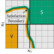
(a) After four Splits.

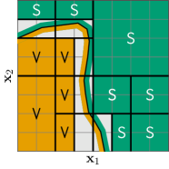
(b) After 17 Splits.

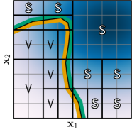
(c) Probability Density Function.

Figure 1: Computing Bounds on Probabilities. This figure illustrates the steps for computing bounds on $p=\mathbb{P}_{\mathbf{x}}{\mathchoice{\left[g_{\mathrm{Sat}}(\mathbf{x},\mathsf{net}(\mathbf{x}))\geq 0\right]}{[g_{\mathrm{Sat}}(\mathbf{x},\mathsf{net}(\mathbf{x}))\geq 0]}{\left[g_{\mathrm{Sat}}(\mathbf{x},\mathsf{net}(\mathbf{x}))\geq 0\right]}{\left[g_{\mathrm{Sat}}(\mathbf{x},\mathsf{net}(\mathbf{x}))\geq 0\right]}}$. Our algorithm successively splits the input space to find regions that do not intersect the satisfaction boundary $g_{\mathrm{Sat}}(\mathbf{x},\mathsf{net}(\mathbf{x}))\geq 0$ (orange/green line  ). Green, orange, and grey rectangles ( / / ) denote regions for which we could prove $g_{\mathrm{Sat}}(\mathbf{x},\mathsf{net}(\mathbf{x}))\geq 0$ (satisfaction)  , $g_{\mathrm{Sat}}(\mathbf{x},\mathsf{net}(\mathbf{x}))<0$ (violation)  , or neither  , respectively. By integrating the probability density $f_{\mathbf{x}}$ in 1(c) (darker means higher density) over the green rectangles  , we obtain a lower bound on $p$. Similarly, we can integrate over the orange rectangles  to construct an upper bound on $p$. Refining the input splitting from 1(a) to 1(b) tightens the bounds on $p$.

4.1 Probabilistic Verification Algorithm

Algorithm 3 describes the PV algorithm. The centrepiece of PV is the procedure ProbabilityBounds for computing bounds $\ell_{i}^{(t)}\leq p_{i}\leq u_{i}^{(t)}$ on a probability $p_{i}$ from Equation 3. Given $\ell_{i}^{(t)}\leq p_{i}\leq u_{i}^{(t)}$, we apply interval arithmetic as introduced in Section 3.2.1 to prove or disprove $f_{\mathrm{Sat}}(p_{1},\ldots,p_{v})$. As described in Section 3.2.1, this analysis may be inconclusive. In this case, ProbabilityBounds refines $\ell_{i}^{(t)},u_{i}^{(t)}$ to obtain $\ell_{i}^{(t+1)},u_{i}^{(t+1)}$ with $\ell_{i}^{(t)}\leq\ell_{i}^{(t+1)}\leq p_{i}\leq u_{i}^{(t+1)}\leq u_{i}^{(t)}$. We again apply interval arithmetic to $f_{\mathrm{Sat}}(p_{1},\ldots,p_{v})$, this time using $\ell_{i}^{(t+1)},u_{i}^{(t+1)}$. If the result remains inconclusive, we iterate refining the bounds on each $p_{i}$ until we obtain a conclusive result. PV applies ProbabilityBounds for each $p_{i}$ in parallel, making use of several CPU cores or several GPUs. Our main contribution is the ProbabilityBounds algorithm for computing a converging sequence of lower and upper bounds on $p_{i}$. Section 4.2 describes ProbabilityBounds in detail.

Input: Probabilistic Verification Problem as in Equation 3, Batch Size $N$

1 for $i\in\{1,\ldots,v\}$ do (Launch $v$ parallel instances of ProbabilityBounds)

2      ${P\!B}_{i}\leftarrow$ Launch $\textsf{ProbabilityBounds}(p_{i},N)$

3      

4for $t\in\mathbb{N}$ do

5      for $i\in\{1,\ldots,v\}$ do Gather $\ell_{i}^{(t)},u_{i}^{(t)}$ from ${P\!B}_{i}$

6       $\ell^{(t)},u^{(t)}\leftarrow\textsf{IntervalArithmetic}(f_{\mathrm{Sat}},(\ell_{1}^{(t)},u_{1}^{(t)}),\ldots,(\ell_{v}^{(t)},u_{v}^{(t)}))$

7       if $\ell^{(t)}\geq 0$ then return Satisfied

8       if $u^{(t)}<0$ then return Violated

9      

Algorithm 3 Probabilistic Verification (PV)

Input: Probability $\mathbb{P}_{\mathbf{x}}{\mathchoice{\left[g_{\mathrm{Sat}}(\mathbf{x},\mathsf{net}(\mathbf{x}))\geq 0\right]}{[g_{\mathrm{Sat}}(\mathbf{x},\mathsf{net}(\mathbf{x}))\geq 0]}{\left[g_{\mathrm{Sat}}(\mathbf{x},\mathsf{net}(\mathbf{x}))\geq 0\right]}{\left[g_{\mathrm{Sat}}(\mathbf{x},\mathsf{net}(\mathbf{x}))\geq 0\right]}}$, Batch Size $N$

$\mathrm{branches}\leftarrow\{\mathcal{X}\}$

  ($\mathcal{X}$ is the input space of $\mathsf{net}$)

1 $\ell^{(0)}\leftarrow 0,u^{(0)}\leftarrow 1$

2 for $t\in\mathbb{N}$ do

      $\mathrm{batch}\leftarrow\textsf{Select}(\mathrm{branches},N)$

        (e.g., branches $\mathcal{B}_{i}$ with largest $\mathbb{P}_{\mathbf{x}}{\mathchoice{\left[\mathcal{B}_{i}\right]}{[\mathcal{B}_{i}]}{\left[\mathcal{B}_{i}\right]}{\left[\mathcal{B}_{i}\right]}}$)

3       $(\underline{\mathbf{y}},\overline{\mathbf{y}})\leftarrow\textsf{ComputeBounds}(g_{\mathrm{Sat}}(\cdot,\mathsf{net}(\cdot)),\mathrm{batch})$

4       $(\mathrm{batch},{\mathcal{X}}_{sat}^{(t)},{\mathcal{X}}_{viol}^{(t)})\leftarrow\textsf{Prune}{}(\mathrm{batch},\underline{\mathbf{y}},\overline{\mathbf{y}})$

5       $\ell^{(t)}\leftarrow\ell^{(t-1)}+\mathbb{P}_{\mathbf{x}}{\mathchoice{\left[{\mathcal{X}}_{sat}^{(t)}\right]}{[{\mathcal{X}}_{sat}^{(t)}]}{\left[{\mathcal{X}}_{sat}^{(t)}\right]}{\left[{\mathcal{X}}_{sat}^{(t)}\right]}}$

6       $u^{(t)}\leftarrow u^{(t-1)}-\mathbb{P}_{\mathbf{x}}{\mathchoice{\left[{\mathcal{X}}_{viol}^{(t)}\right]}{[{\mathcal{X}}_{viol}^{(t)}]}{\left[{\mathcal{X}}_{viol}^{(t)}\right]}{\left[{\mathcal{X}}_{viol}^{(t)}\right]}}$

       yield $\ell^{(t)},u^{(t)}$

        (Report new bounds to PV)

       $\mathrm{new}\leftarrow\textsf{Split}{}(\mathrm{batch})$

        (e.g., BaBSB [BunelLuTurkaslanEtAl2020])

7       $\mathrm{branches}\leftarrow(\mathrm{branches}\setminus\mathrm{batch})\cup\mathrm{new}$

8      

Algorithm 4 ProbabilityBounds

4.2 Bounding Probabilities

Our ProbabilityBounds algorithm for deriving and refining bounds on a probability is described in detail in Algorithm 4 and illustrated in Figure 1. ProbabilityBounds is a massively parallel input-splitting branch and bound procedure that leverages a bound propagation algorithm for non-probabilistic neural network verification (ComputeBounds). Since we only consider a single probability $p_{i}$ as in Equation 3 in this section, we denote this probability as $p=\mathbb{P}_{\mathbf{x}}{\mathchoice{\left[g_{\mathrm{Sat}}(\mathbf{x},\mathsf{net}(\mathbf{x}))\geq 0\right]}{[g_{\mathrm{Sat}}(\mathbf{x},\mathsf{net}(\mathbf{x}))\geq 0]}{\left[g_{\mathrm{Sat}}(\mathbf{x},\mathsf{net}(\mathbf{x}))\geq 0\right]}{\left[g_{\mathrm{Sat}}(\mathbf{x},\mathsf{net}(\mathbf{x}))\geq 0\right]}}$.

ProbabilityBounds receives $p$ and a batch size $N\in\mathbb{N}$ as input. The algorithm iteratively computes $\ell^{(t)},u^{(t)}\in[0,1]$, such that $\ell^{(t)}\leq\ell^{(t^{\prime})}\leq p\leq u^{(t^{\prime})}\leq u^{(t)}$, $\forall t,t^{\prime}\in\mathbb{N},t^{\prime}\geq t$. The following sections describe each step of ProbabilityBounds in detail.

4.2.1 Initialisation

Initially, we consider a single branch encompassing $\mathsf{net}$’s entire input space $\mathcal{X}$. As in Section 3, we assume $\mathcal{X}$ to be a bounded hyperrectangle. We use the trivial bounds $\ell^{(0)}=0\leq p\leq 1=u^{(0)}$ as initial bounds on $p$.

4.2.2 Selecting Branches

First, we select a batch of $N\in\mathbb{N}$ branches. In the spirit of [XuZhangWangEtAl2021], we leverage the data parallelism of modern CPUs and GPUs to process several branches at once. In iteration $t=1$, the batch only contains the branch $\mathcal{X}$. Which branches we select determines how fast we obtain tight bounds on $p$. We propose two heuristics for selecting branches:

• SelectProb: Inspired by FairSquare [AlbarghouthiDAntoniDrewsEtAl2017], this heuristic selects the $N$ branches $\mathcal{B}_{i}$ with the largest $\mathbb{P}_{\mathbf{x}}{\mathchoice{\left[\mathcal{B}_{i}\right]}{[\mathcal{B}_{i}]}{\left[\mathcal{B}_{i}\right]}{\left[\mathcal{B}_{i}\right]}}$. This heuristic is motivated by the observation that pruning these branches would lead to the largest improvement of $\ell^{(t)},u^{(t)}$.

• SelectProbLogBounds: This heuristic selects the $N$ branches $\mathcal{B}_{i}$ with the largest $\frac{\mathbb{P}_{\mathbf{x}}{\mathchoice{\left[\mathcal{B}_{i}\right]}{[\mathcal{B}_{i}]}{\left[\mathcal{B}_{i}\right]}{\left[\mathcal{B}_{i}\right]}}}{\log(e+\overline{\mathbf{y}}_{i}-\underline{\mathbf{y}}_{i})}$ where $\underline{\mathbf{y}},\overline{\mathbf{y}}$ are as in ProbabilityBounds. The motivation for this heuristic is to select the branches with the largest probability while $\underline{\mathbf{y}},\overline{\mathbf{y}}$ are loose to focus on the most relevant regions of the input space, but greedily select branches that have tight bounds with the expectation that these will be pruned soon.

We compare SelectProb and SelectProbLogBounds experimentally in LABEL:sec:heuristics-additional. The comparison reveals that SelectProbLogBounds slightly speeds up PV compared to SelectProb.

4.2.3 Pruning

The next step is to prune those branches $\mathcal{B}_{j}\in\mathrm{batch}$, for which we can determine that $y=g_{\mathrm{Sat}}(\mathbf{x},\mathsf{net}(\mathbf{x}))\geq 0$ is either certainly satisfied or certainly violated. For this, we first compute $\underline{\mathbf{y}}\leq g_{\mathrm{Sat}}(\cdot,\mathsf{net}(\cdot))\leq\overline{\mathbf{y}}$ for the entire $\mathrm{batch}$ using a sound neural network verifier like interval arithmetic, CROWN [ZhangWengChenEtAl2018], or $\alpha$-CROWN [XuZhangWangEtAl2021]. If $\underline{\mathbf{y}}_{j}\geq 0$ ($y\geq 0$ is certainly satisfied) or $\overline{\mathbf{y}}_{j}<0$ ($y\geq 0$ is certainly violated), we can prune $\mathcal{B}_{j}$ analogously to Algorithm 2. We collect the branches with $\underline{\mathbf{y}}_{j}\geq 0$ in the set ${\mathcal{X}}_{sat}^{(t)}$ and the branches with $\overline{\mathbf{y}}_{j}<0$ in ${\mathcal{X}}_{viol}^{(t)}$, where $t\in\mathbb{N}$ is the current iteration.

4.2.4 Updating Bounds

Let ${\hat{\mathcal{X}}}_{sat}^{(t)}=\bigcup_{t^{\prime}=1}^{t}{\mathcal{X}}_{sat}^{(t^{\prime})}$ and ${\hat{\mathcal{X}}}_{viol}^{(t)}=\bigcup_{t^{\prime}=1}^{t}{\mathcal{X}}_{viol}^{(t^{\prime})}$, where $t\in\mathbb{N}$ is the current iteration. Then, $\ell^{(t)}=\mathbb{P}_{\mathbf{x}}{\mathchoice{\left[{\hat{\mathcal{X}}}_{sat}^{(t)}\right]}{[{\hat{\mathcal{X}}}_{sat}^{(t)}]}{\left[{\hat{\mathcal{X}}}_{sat}^{(t)}\right]}{\left[{\hat{\mathcal{X}}}_{sat}^{(t)}\right]}}\leq p$. Similarly, $\mathdcal{k}^{(t)}=\mathbb{P}_{\mathbf{x}}{\mathchoice{\left[{\hat{\mathcal{X}}}_{viol}^{(t)}\right]}{[{\hat{\mathcal{X}}}_{viol}^{(t)}]}{\left[{\hat{\mathcal{X}}}_{viol}^{(t)}\right]}{\left[{\hat{\mathcal{X}}}_{viol}^{(t)}\right]}}\leq\mathbb{P}_{\mathbf{x}}{\mathchoice{\left[f_{\mathrm{Sat}}(\mathbf{x},\mathsf{net}(\mathbf{x}))<0\right]}{[f_{\mathrm{Sat}}(\mathbf{x},\mathsf{net}(\mathbf{x}))<0]}{\left[f_{\mathrm{Sat}}(\mathbf{x},\mathsf{net}(\mathbf{x}))<0\right]}{\left[f_{\mathrm{Sat}}(\mathbf{x},\mathsf{net}(\mathbf{x}))<0\right]}}=1-p$. Therefore, $1-\mathdcal{k}^{(t)}=u^{(t)}\geq p$. Practically, we only have to maintain the current bounds $\ell^{(t)}$ and $u^{(t)}$ instead of the sets ${\hat{\mathcal{X}}}_{sat}^{(t)}$ and ${\hat{\mathcal{X}}}_{viol}^{(t)}$.

Because ${\hat{\mathcal{X}}}_{sat}^{(t)}$ and ${\hat{\mathcal{X}}}_{viol}^{(t)}$ are a union of disjoint hyperrectangles, exactly computing $\mathbb{P}_{\mathbf{x}}{\mathchoice{\left[{\hat{\mathcal{X}}}_{sat}^{(t)}\right]}{[{\hat{\mathcal{X}}}_{sat}^{(t)}]}{\left[{\hat{\mathcal{X}}}_{sat}^{(t)}\right]}{\left[{\hat{\mathcal{X}}}_{sat}^{(t)}\right]}}$ and $\mathbb{P}_{\mathbf{x}}{\mathchoice{\left[{\hat{\mathcal{X}}}_{viol}^{(t)}\right]}{[{\hat{\mathcal{X}}}_{viol}^{(t)}]}{\left[{\hat{\mathcal{X}}}_{viol}^{(t)}\right]}{\left[{\hat{\mathcal{X}}}_{viol}^{(t)}\right]}}$ is feasible for a large class of probability distributions, including discrete, uniform, and univariate continuous distributions, as well as Mixture Models and Bayesian Networks of such distributions, but not, for example, multivariate normal distributions. Practically, one must also accommodate floating point errors in these computations. While we do not address this in this paper, our approach can be extended to this end.

ProbabilityBounds now reports the refined bounds $\ell^{(t)}\leq p\leq u^{(t)}$ to PV, which applies interval arithmetic to determine whether $\mathsf{net}$ is feasible for the probabilistic verification problem. If this remains inconclusive, we proceed with splitting the selected branches.

4.2.5 Splitting

Splitting refines a branch $\mathcal{B}=[\underline{\mathbf{x}missing},\overline{\mathbf{x}}]$ by selecting a dimension $d\in\{1,\ldots,n\}$ to split. We first describe how $d$ is split before discussing how to select $d$. A dimension can encode several types of variables. We consider continuous variables, such as normalised pixel values, integer variables, such as age, and dimensions containing one indicator of a one-hot encoded categorical variable like gender. The type of variable encoded in $d$ determines how we split $d$.

• For a continuous variable, we bisect $\mathcal{B}$ along $d$ resulting in two new branches $[\underline{\mathbf{x}missing}^{\prime},\overline{\mathbf{x}}^{\prime}]$ and $[\underline{\mathbf{x}missing}^{\prime\prime},\overline{\mathbf{x}}^{\prime\prime}]$. Concretely, $\underline{\mathbf{x}missing}^{\prime}_{d^{\prime}}=\underline{\mathbf{x}missing}^{\prime\prime}_{d^{\prime}}=\underline{\mathbf{x}missing}_{d^{\prime}}$ and $\overline{\mathbf{x}}^{\prime}_{d^{\prime}}=\overline{\mathbf{x}}^{\prime\prime}_{d^{\prime}}=\overline{\mathbf{x}}_{d^{\prime}}$ for all $d^{\prime}\in\{1,\ldots,n\}\setminus\{d\}$ while $\overline{\mathbf{x}}^{\prime}_{d}=\underline{\mathbf{x}missing}^{\prime\prime}_{d}=(\underline{\mathbf{x}missing}_{d}+\overline{\mathbf{x}}_{d})/2$, $\underline{\mathbf{x}missing}^{\prime}_{d}=\underline{\mathbf{x}missing}_{d}$, and $\overline{\mathbf{x}}^{\prime\prime}_{d}=\overline{\mathbf{x}}_{d}$.

• For integer variables, we bisect along $d$ to obtain $[\underline{\mathbf{x}missing}^{\prime},\overline{\mathbf{x}}^{\prime}]$, $[\underline{\mathbf{x}missing}^{\prime\prime},\overline{\mathbf{x}}^{\prime\prime}]$ and round $\overline{\mathbf{x}}^{\prime}_{d}$ to the next smaller integer while rounding $\underline{\mathbf{x}missing}^{\prime\prime}_{d}$ to the next larger integer.

• For a one-hot encoded categorical variable $A$ encoded in the dimensions $D\in\{1,\ldots,n\}$ with $d\in D$, we create one split where $A$ is equal to the category represented by $d$ and one where $A$ is different from this category. Formally, $\underline{\mathbf{x}}_{d}^{\prime}=\overline{\mathbf{x}}_{d}^{\prime}=1$ and $\underline{\mathbf{x}}_{d^{\prime}}^{\prime}=\overline{\mathbf{x}}_{d^{\prime}}^{\prime}=0$ for $d^{\prime}\in D\setminus\{d\}$ defines $[\underline{\mathbf{x}}^{\prime},\overline{\mathbf{x}}^{\prime}]$. For $[\underline{\mathbf{x}}^{\prime\prime},\overline{\mathbf{x}}^{\prime\prime}]$, we set $\underline{\mathbf{x}}_{d}^{\prime\prime}=\overline{\mathbf{x}}_{d}^{\prime\prime}=0$ and leave the remaining values are they are in $\underline{\mathbf{x}}$ and $\overline{\mathbf{x}}$.

In any case, we need to ensure not to select $d$ if $\underline{\mathbf{x}missing}_{d}=\overline{\mathbf{x}}_{d}$. We introduce two heuristics for selecting a dimension:

• LongestEdge: This well-known heuristic [BunelLuTurkaslanEtAl2020] selects the dimension with the largest edge length $\overline{\mathbf{x}}_{d}-\underline{\mathbf{x}missing}_{d}$.

• BaBSB: We use a variant of the BaBSB heuristic of [BunelLuTurkaslanEtAl2020]. The idea of BaBSB is to estimate the improvement in bounds that splitting dimension $d$ yields by using a yet less expensive technique than ComputeBounds. Our variant of BaBSB uses interval arithmetic, assuming that we use CROWN or $\alpha$-CROWN for ComputeBounds. Let $[\underline{\mathbf{x}missing}^{(d,1)},\overline{\mathbf{x}}^{(d,1)}]$ and $[\underline{\mathbf{x}missing}^{(d,2)},\overline{\mathbf{x}}^{(d,2)}]$ be the two new branches originating from splitting dimension $d\in\{1,\ldots,n\}$ and let $\underline{y}^{(d,1)},\overline{y}^{(d,1)}$, $\underline{y}^{(d,2)},\overline{y}^{(d,2)}$ be the bounds that interval arithmetic computes on $g_{\mathrm{Sat}}(\cdot,\mathsf{net}(\cdot))$ for these branches. Our BaBSB selects $d=\operatorname*{arg\,max}_{d\in\{1,\ldots,n\}}\tilde{y}^{(d)}$, where $\tilde{y}^{(d)}=\max(\max(\underline{y}^{(d,1)},\underline{y}^{(d,2)}),-{\min(\overline{y}^{(d,1)},\overline{y}^{(d,2)})})$.

While LongestEdge is more theoretically accessible, BaBSB is practically advantageous, as discussed in LABEL:sec:heuristics-additional.

5 Theoretical Analysis

In this section, we prove that PV is a sound probabilistic verification algorithm when instantiated with a suitable ComputeBounds procedure. We also prove that PV instantiated with SelectProb, LongestEdge, and interval arithmetic for ComputeBounds is complete under mild assumptions on the probabilistic verification problem. Soundness and completeness are defined in 2. As in Section 4.2, we omit index and superscripts when considering only a single probability $p=\mathbb{P}_{\mathbf{x}}{\mathchoice{\left[g_{\mathrm{Sat}}(\mathbf{x},\mathsf{net}(\mathbf{x}))\geq 0\right]}{[g_{\mathrm{Sat}}(\mathbf{x},\mathsf{net}(\mathbf{x}))\geq 0]}{\left[g_{\mathrm{Sat}}(\mathbf{x},\mathsf{net}(\mathbf{x}))\geq 0\right]}{\left[g_{\mathrm{Sat}}(\mathbf{x},\mathsf{net}(\mathbf{x}))\geq 0\right]}}$.

5.1 Soundness

First, we prove that ProbabilityBounds produces sound bounds on $p$ when using a sound ComputeBounds procedure, that is, a procedure that computes valid bounds, such as interval arithmetic or CROWN [ZhangWengChenEtAl2018]. The soundness of PV then follows immediately.

Theorem 1 (Sound Bounds).

Let $N\in\mathbb{N}$ be a batch size and assume ComputeBounds produces valid bounds. Let ${\left((\ell^{(t)},u^{(t)})\right)}_{t\in\mathbb{N}}$ be the iterates of $\textsf{ProbabilityBounds}(\mathbb{P}_{\mathbf{x}}{\mathchoice{\left[g_{\mathrm{Sat}}(\mathbf{x},\mathsf{net}(\mathbf{x}))\geq 0\right]}{[g_{\mathrm{Sat}}(\mathbf{x},\mathsf{net}(\mathbf{x}))\geq 0]}{\left[g_{\mathrm{Sat}}(\mathbf{x},\mathsf{net}(\mathbf{x}))\geq 0\right]}{\left[g_{\mathrm{Sat}}(\mathbf{x},\mathsf{net}(\mathbf{x}))\geq 0\right]}},N)$. It holds that $\ell^{(t)}\leq\mathbb{P}_{\mathbf{x}}{\mathchoice{\left[g_{\mathrm{Sat}}(\mathbf{x},\mathsf{net}(\mathbf{x}))\geq 0\right]}{[g_{\mathrm{Sat}}(\mathbf{x},\mathsf{net}(\mathbf{x}))\geq 0]}{\left[g_{\mathrm{Sat}}(\mathbf{x},\mathsf{net}(\mathbf{x}))\geq 0\right]}{\left[g_{\mathrm{Sat}}(\mathbf{x},\mathsf{net}(\mathbf{x}))\geq 0\right]}}\leq u^{(t)}$ for all $t\in\mathbb{N}$.

Proof.

Let $t\in\mathbb{N}$ and let ${\mathcal{X}}_{sat}^{(t)}$ and ${\mathcal{X}}_{viol}^{(t)}$ be as in Algorithm 4. ProbabilityBounds computes $\ell^{(t)}$ as the total probability of all previously pruned satisfied branches ${\hat{\mathcal{X}}}_{sat}^{(t)}=\bigcup_{t^{\prime}=1}^{t}{\mathcal{X}}_{sat}^{(t^{\prime})}$. Similarly, $u^{(t)}=1-\mathdcal{k}^{(t)}$ where $\mathdcal{k}^{(t)}$ is the total probability of all previously pruned violated branches ${\hat{\mathcal{X}}}_{viol}^{(t)}=\bigcup_{t^{\prime}=1}^{t}{\mathcal{X}}_{viol}^{(t^{\prime})}$. Since we assumed that ComputeBounds produces valid bounds, Prune only prunes branches that are actually satisfied or violated. Therefore, ${\hat{\mathcal{X}}}_{sat}^{(t)}\subseteq\{\mathbf{x}\in\mathcal{X}\mid g_{\mathrm{Sat}}(\mathbf{x},\mathsf{net}(\mathbf{x}))\geq 0\}$ and ${\hat{\mathcal{X}}}_{viol}^{(t)}\subseteq\{\mathbf{x}\in\mathcal{X}\mid g_{\mathrm{Sat}}(\mathbf{x},\mathsf{net}(\mathbf{x}))<0\}$. From this, it follows directly that

$$\ell^{(t)} =\mathbb{P}_{\mathbf{x}}{\mathchoice{\left[{\hat{\mathcal{X}}}_{sat}^{(t)}\right]}{[{\hat{\mathcal{X}}}_{sat}^{(t)}]}{\left[{\hat{\mathcal{X}}}_{sat}^{(t)}\right]}{\left[{\hat{\mathcal{X}}}_{sat}^{(t)}\right]}}\leq\mathbb{P}_{\mathbf{x}}{\mathchoice{\left[g_{\mathrm{Sat}}(\mathbf{x},\mathsf{net}(\mathbf{x}))\geq 0\right]}{[g_{\mathrm{Sat}}(\mathbf{x},\mathsf{net}(\mathbf{x}))\geq 0]}{\left[g_{\mathrm{Sat}}(\mathbf{x},\mathsf{net}(\mathbf{x}))\geq 0\right]}{\left[g_{\mathrm{Sat}}(\mathbf{x},\mathsf{net}(\mathbf{x}))\geq 0\right]}}$$

$$\mathdcal{k}^{(t)} =\mathbb{P}_{\mathbf{x}}{\mathchoice{\left[{\hat{\mathcal{X}}}_{viol}^{(t)}\right]}{[{\hat{\mathcal{X}}}_{viol}^{(t)}]}{\left[{\hat{\mathcal{X}}}_{viol}^{(t)}\right]}{\left[{\hat{\mathcal{X}}}_{viol}^{(t)}\right]}}\leq\mathbb{P}_{\mathbf{x}}{\mathchoice{\left[g_{\mathrm{Sat}}(\mathbf{x},\mathsf{net}(\mathbf{x}))<0\right]}{[g_{\mathrm{Sat}}(\mathbf{x},\mathsf{net}(\mathbf{x}))<0]}{\left[g_{\mathrm{Sat}}(\mathbf{x},\mathsf{net}(\mathbf{x}))<0\right]}{\left[g_{\mathrm{Sat}}(\mathbf{x},\mathsf{net}(\mathbf{x}))<0\right]}},$$

which implies $u^{(t)}=1-\mathdcal{k}^{(t)}\geq 1-\mathbb{P}_{\mathbf{x}}{\mathchoice{\left[g_{\mathrm{Sat}}(\mathbf{x},\mathsf{net}(\mathbf{x}))<0\right]}{[g_{\mathrm{Sat}}(\mathbf{x},\mathsf{net}(\mathbf{x}))<0]}{\left[g_{\mathrm{Sat}}(\mathbf{x},\mathsf{net}(\mathbf{x}))<0\right]}{\left[g_{\mathrm{Sat}}(\mathbf{x},\mathsf{net}(\mathbf{x}))<0\right]}}=\mathbb{P}_{\mathbf{x}}{\mathchoice{\left[g_{\mathrm{Sat}}(\mathbf{x},\mathsf{net}(\mathbf{x}))\geq 0\right]}{[g_{\mathrm{Sat}}(\mathbf{x},\mathsf{net}(\mathbf{x}))\geq 0]}{\left[g_{\mathrm{Sat}}(\mathbf{x},\mathsf{net}(\mathbf{x}))\geq 0\right]}{\left[g_{\mathrm{Sat}}(\mathbf{x},\mathsf{net}(\mathbf{x}))\geq 0\right]}}$. This shows that ProbabilityBounds is sound. ∎

Corollary 1 (Soundness).

PV is sound when using a ComputeBounds procedure that computes valid bounds.

Proof.

Corollary 1 follows from Theorem 1 and the soundness of interval arithmetic [MooreKearfottCloud2009, Theorem 5.1]. ∎

5.2 Completeness

We study the completeness of PV. Concretely, we prove that PV instantiated with SelectProb, interval arithmetic for ComputeBounds, and LongestEdge is complete under a mildly restrictive condition on Equation 3.

Assumption 1.

Let $v$, $f_{\mathrm{Sat}}$, $g_{\mathrm{Sat}}^{(i)}$, and $\mathbf{x}^{(i)}$ be as in Equation 3. Assume $f_{\mathrm{Sat}}(p_{1},\ldots,p_{v})\neq 0$ and $\forall i\in\{1,\ldots,v\}:\mathbb{P}_{\mathbf{x}^{(i)}}{\mathchoice{\left[g_{\mathrm{Sat}}^{(i)}(\mathbf{x}^{(i)},\mathsf{net}(\mathbf{x}^{(i)})){}=0\right]}{[g_{\mathrm{Sat}}^{(i)}(\mathbf{x}^{(i)},\mathsf{net}(\mathbf{x}^{(i)})){}=0]}{\left[g_{\mathrm{Sat}}^{(i)}(\mathbf{x}^{(i)},\mathsf{net}(\mathbf{x}^{(i)})){}=0\right]}{\left[g_{\mathrm{Sat}}^{(i)}(\mathbf{x}^{(i)},\mathsf{net}(\mathbf{x}^{(i)})){}=0\right]}}=0$.

To prove the completeness of PV, we first establish that ProbabilityBounds produces a sequence of lower and upper bounds that converge towards each other. Intuitively, we require 1 since converging bounds on $f_{\mathrm{Sat}}(p_{1},\ldots,p_{n})$ are insufficient for proving $f_{\mathrm{Sat}}(p_{1},\ldots,p_{n})\geq 0$ if $f_{\mathrm{Sat}}(p_{1},\ldots,p_{n})=0$ [AlbarghouthiDAntoniDrewsEtAl2017]. However, excluding $f_{\mathrm{Sat}}(p_{1},\ldots,p_{v})=0$ is only mildly restrictive as we can always tighten the constraint to $f_{\mathrm{Sat}}(p_{1},\ldots,p_{n})\geq\varepsilon$ for an arbitrarily small $\varepsilon>0$. The second assumption $\mathbb{P}_{\mathbf{x}}{\mathchoice{\left[g_{\mathrm{Sat}}(\mathbf{x},\mathsf{net}(\mathbf{x})){}=0\right]}{[g_{\mathrm{Sat}}(\mathbf{x},\mathsf{net}(\mathbf{x})){}=0]}{\left[g_{\mathrm{Sat}}(\mathbf{x},\mathsf{net}(\mathbf{x})){}=0\right]}{\left[g_{\mathrm{Sat}}(\mathbf{x},\mathsf{net}(\mathbf{x})){}=0\right]}}=0$ is only mildly restrictive for similar reasons. In particular, we can tighten $\mathbb{P}_{\mathbf{x}}{\mathchoice{\left[g_{\mathrm{Sat}}(\mathbf{x},\mathsf{net}(\mathbf{x}))\geq 0\right]}{[g_{\mathrm{Sat}}(\mathbf{x},\mathsf{net}(\mathbf{x}))\geq 0]}{\left[g_{\mathrm{Sat}}(\mathbf{x},\mathsf{net}(\mathbf{x}))\geq 0\right]}{\left[g_{\mathrm{Sat}}(\mathbf{x},\mathsf{net}(\mathbf{x}))\geq 0\right]}}$ to $\mathbb{P}_{\mathbf{x}}{\mathchoice{\left[g_{\mathrm{Sat}}(\mathbf{x},\mathsf{net}(\mathbf{x})){}\geq\varepsilon\right]}{[g_{\mathrm{Sat}}(\mathbf{x},\mathsf{net}(\mathbf{x})){}\geq\varepsilon]}{\left[g_{\mathrm{Sat}}(\mathbf{x},\mathsf{net}(\mathbf{x})){}\geq\varepsilon\right]}{\left[g_{\mathrm{Sat}}(\mathbf{x},\mathsf{net}(\mathbf{x})){}\geq\varepsilon\right]}}$ for $\varepsilon>0$ such that $\mathbb{P}_{\mathbf{x}}{\mathchoice{\left[g_{\mathrm{Sat}}(\mathbf{x},\mathsf{net}(\mathbf{x})){}=\varepsilon\right]}{[g_{\mathrm{Sat}}(\mathbf{x},\mathsf{net}(\mathbf{x})){}=\varepsilon]}{\left[g_{\mathrm{Sat}}(\mathbf{x},\mathsf{net}(\mathbf{x})){}=\varepsilon\right]}{\left[g_{\mathrm{Sat}}(\mathbf{x},\mathsf{net}(\mathbf{x})){}=\varepsilon\right]}}=0$. Such a $\varepsilon>0$ exists because $\mathbb{P}_{\mathbf{x}}{\mathchoice{\left[g_{\mathrm{Sat}}(\mathbf{x},\mathsf{net}(\mathbf{x})){}=0\right]}{[g_{\mathrm{Sat}}(\mathbf{x},\mathsf{net}(\mathbf{x})){}=0]}{\left[g_{\mathrm{Sat}}(\mathbf{x},\mathsf{net}(\mathbf{x})){}=0\right]}{\left[g_{\mathrm{Sat}}(\mathbf{x},\mathsf{net}(\mathbf{x})){}=0\right]}}=0$ means that the satisfaction boundary has positive volume, but any neural network has only finitely many flat regions that can produce a satisfaction boundary of positive volume.

Lemma 1 (Converging Probability Bounds).

Let $N\in\mathbb{N}$ be a batch size. Let ${\left((\ell^{(t)},u^{(t)})\right)}_{t\in\mathbb{N}}$ be the iterates of $\textsf{ProbabilityBounds}{}(\mathbb{P}_{\mathbf{x}}{\mathchoice{\left[g_{\mathrm{Sat}}(\mathbf{x},\mathsf{net}(\mathbf{x}))\geq 0\right]}{[g_{\mathrm{Sat}}(\mathbf{x},\mathsf{net}(\mathbf{x}))\geq 0]}{\left[g_{\mathrm{Sat}}(\mathbf{x},\mathsf{net}(\mathbf{x}))\geq 0\right]}{\left[g_{\mathrm{Sat}}(\mathbf{x},\mathsf{net}(\mathbf{x}))\geq 0\right]}},N)$ instantiated with SelectProb, interval arithmetic for ComputeBounds and LongestEdge. Assume $\mathbb{P}_{\mathbf{x}}{\mathchoice{\left[g_{\mathrm{Sat}}(\mathbf{x},\mathsf{net}(\mathbf{x}))=0\right]}{[g_{\mathrm{Sat}}(\mathbf{x},\mathsf{net}(\mathbf{x}))=0]}{\left[g_{\mathrm{Sat}}(\mathbf{x},\mathsf{net}(\mathbf{x}))=0\right]}{\left[g_{\mathrm{Sat}}(\mathbf{x},\mathsf{net}(\mathbf{x}))=0\right]}}=0$ as in 1. Then,

$$\lim_{t\to\infty}\ell^{(t)}=\lim_{t\to\infty}u^{(t)}=\mathbb{P}_{\mathbf{x}}{\mathchoice{\left[g_{\mathrm{Sat}}(\mathbf{x},\mathsf{net}(\mathbf{x}))\geq 0\right]}{[g_{\mathrm{Sat}}(\mathbf{x},\mathsf{net}(\mathbf{x}))\geq 0]}{\left[g_{\mathrm{Sat}}(\mathbf{x},\mathsf{net}(\mathbf{x}))\geq 0\right]}{\left[g_{\mathrm{Sat}}(\mathbf{x},\mathsf{net}(\mathbf{x}))\geq 0\right]}}.$$

Purely Discrete Input Spaces.

In the following, we assume that the input space $\mathcal{X}$ of $\mathsf{net}$ contains at least one continuous variable. Otherwise, $\mathcal{X}$ contains only finitely many discrete values. This implies that ProbabilityBounds eventually reaches an iteration where no branch can be split further. However, in this iteration, all branches are points in the input space, for which interval arithmetic computes $\underline{\mathbf{y}}=\overline{\mathbf{y}}$ [MooreKearfottCloud2009, see LABEL:sec:ia-theorem-six-one-moore-et-al]. In turn, this implies that all branches are pruned, making ProbabilityBounds complete.

We require the following intermediate result for proving Lemma 1. We write $\mathcal{B}\leadsto\mathcal{B}_{t}$ if $\mathcal{B}_{t}$ is a branch in iteration $t$ of ProbabilityBounds that originates from splitting $\mathcal{B}$, meaning that $\mathcal{B}_{t}\subset\mathcal{B}$.

Lemma 2.

Let $N\in\mathbb{N}$. ProbabilityBounds instantiated as in Lemma 1 satisfies

$$\forall t\in\mathbb{N}:\forall\mathcal{B}\in\mathrm{branches}^{(t)}:\mathbb{P}_{\mathbf{x}}{\mathchoice{\left[\mathcal{B}\right]}{[\mathcal{B}]}{\left[\mathcal{B}\right]}{\left[\mathcal{B}\right]}}>0\Longrightarrow\exists t^{\prime}\geq t:\mathcal{B}\in\textsf{SelectProb}{}(\mathrm{branches}^{(t^{\prime})},N),$$

where $\mathrm{branches}^{(t)}$ is the value of the $\mathrm{branches}$ variable of ProbabilityBounds in iteration $t$.

Proof.

Let $N\in\mathbb{N}$ and let $\mathcal{B}\notin\textsf{SelectProb}{}(\mathrm{branches}^{(t)},N)$ in iteration $t\in\mathbb{N}$ of ProbabilityBounds with $\mathbb{P}_{\mathbf{x}}{\mathchoice{\left[\mathcal{B}\right]}{[\mathcal{B}]}{\left[\mathcal{B}\right]}{\left[\mathcal{B}\right]}}>0$. There are at least $N$ branches $\mathcal{B}_{t}^{\prime}$ in iteration $t$ with $\mathbb{P}_{\mathbf{x}}{\mathchoice{\left[\mathcal{B}_{t}^{\prime}\right]}{[\mathcal{B}_{t}^{\prime}]}{\left[\mathcal{B}_{t}^{\prime}\right]}{\left[\mathcal{B}_{t}^{\prime}\right]}}\geq\mathbb{P}_{\mathbf{x}}{\mathchoice{\left[\mathcal{B}\right]}{[\mathcal{B}]}{\left[\mathcal{B}\right]}{\left[\mathcal{B}\right]}}$. We show

$$\exists t^{\prime}>t:\forall\mathcal{B}_{t}^{\prime},\mathbb{P}_{\mathbf{x}}{\mathchoice{\left[\mathcal{B}_{t}^{\prime}\right]}{[\mathcal{B}_{t}^{\prime}]}{\left[\mathcal{B}_{t}^{\prime}\right]}{\left[\mathcal{B}_{t}^{\prime}\right]}}\geq\mathbb{P}_{\mathbf{x}}{\mathchoice{\left[\mathcal{B}\right]}{[\mathcal{B}]}{\left[\mathcal{B}\right]}{\left[\mathcal{B}\right]}}:\underbrace{\forall\mathcal{B}_{t^{\prime}}^{\prime},\mathcal{B}_{t}^{\prime}\leadsto\mathcal{B}_{t^{\prime}}^{\prime}:\mathbb{P}_{\mathbf{x}}{\mathchoice{\left[\mathcal{B}_{t^{\prime}}^{\prime}\right]}{[\mathcal{B}_{t^{\prime}}^{\prime}]}{\left[\mathcal{B}_{t^{\prime}}^{\prime}\right]}{\left[\mathcal{B}_{t^{\prime}}^{\prime}\right]}}<\mathbb{P}_{\mathbf{x}}{\mathchoice{\left[\mathcal{B}\right]}{[\mathcal{B}]}{\left[\mathcal{B}\right]}{\left[\mathcal{B}\right]}}}_{(\ast)}.$$ (5)

Let $\mathcal{B}_{t}^{\prime}$ be a branch in iteration $t$ with $\mathbb{P}_{\mathbf{x}}{\mathchoice{\left[\mathcal{B}_{t}^{\prime}\right]}{[\mathcal{B}_{t}^{\prime}]}{\left[\mathcal{B}_{t}^{\prime}\right]}{\left[\mathcal{B}_{t}^{\prime}\right]}}\geq\mathbb{P}_{\mathbf{x}}{\mathchoice{\left[\mathcal{B}_{t}\right]}{[\mathcal{B}_{t}]}{\left[\mathcal{B}_{t}\right]}{\left[\mathcal{B}_{t}\right]}}$. We first show that there is an iteration $t^{\prime}>t$ such that $(\ast)$ holds for $\mathcal{B}_{t}^{\prime}$.

First of all, if $\mathcal{B}_{t}^{\prime}$ is pruned by ProbabilityBounds in iteration $t$, then there are no new branches originating from $\mathcal{B}_{t}^{\prime}$, so that $(\ast)$ holds vacuously. Otherwise, ProbabilityBounds splits $\mathcal{B}_{t}^{\prime}$.

Without loss of generality, assume that the dimension selected for splitting encodes a continuous variable. This does not harm generality since discrete variables in a bounded input space can only be split finitely often and will, therefore, eventually become unavailable for splitting. Since we split continuous variables by bisection, we have that the volume of all branches $\mathcal{B}_{t^{\prime}}^{\prime}$ originating from $\mathcal{B}_{t}^{\prime}$ decreases towards zero as $t^{\prime}$ increases.

As stated in Section 3, we assume that all continuous random variables admit a probability density function. This implies that the probability in all branches $\mathcal{B}_{t^{\prime}}^{\prime}$ originating from $\mathcal{B}_{t}^{\prime}$ decreases towards zero as the volume decreases towards zero. Therefore, there is a $t^{\prime}$, such that $(\ast)$ is satisfied for $\mathcal{B}_{t}^{\prime}$. Since there are only finitely many branches in any iteration of ProbabilityBounds, the above implies that Equation 5 is satisfied. In turn, this directly implies that $\mathcal{B}$ is eventually selected by ProbabilityBounds, proving Lemma 2. ∎

Proof of Lemma 1.

We first prove that $\lim_{t\to\infty}\ell^{(t)}=\mathbb{P}_{\mathbf{x}}{\mathchoice{\left[g_{\mathrm{Sat}}(\mathbf{x},\mathsf{net}(\mathbf{x}))\geq 0\right]}{[g_{\mathrm{Sat}}(\mathbf{x},\mathsf{net}(\mathbf{x}))\geq 0]}{\left[g_{\mathrm{Sat}}(\mathbf{x},\mathsf{net}(\mathbf{x}))\geq 0\right]}{\left[g_{\mathrm{Sat}}(\mathbf{x},\mathsf{net}(\mathbf{x}))\geq 0\right]}}$. The convergence of the upper bound, $\lim_{t\to\infty}u^{(t)}=\mathbb{P}_{\mathbf{x}}{\mathchoice{\left[g_{\mathrm{Sat}}(\mathbf{x},\mathsf{net}(\mathbf{x}))\geq 0\right]}{[g_{\mathrm{Sat}}(\mathbf{x},\mathsf{net}(\mathbf{x}))\geq 0]}{\left[g_{\mathrm{Sat}}(\mathbf{x},\mathsf{net}(\mathbf{x}))\geq 0\right]}{\left[g_{\mathrm{Sat}}(\mathbf{x},\mathsf{net}(\mathbf{x}))\geq 0\right]}}$ follows with a similar argument.

Let ${\mathcal{X}}_{sat}^{\ast}=\{\mathbf{x}\in\mathcal{X}\mid g_{\mathrm{Sat}}(\mathbf{x},\mathsf{net}(\mathbf{x}))>0\}$, where $\mathcal{X}$ is the input space of $\mathsf{net}$. Note that $\mathbb{P}_{\mathbf{x}}{\mathchoice{\left[{\mathcal{X}}_{sat}^{\ast}\right]}{[{\mathcal{X}}_{sat}^{\ast}]}{\left[{\mathcal{X}}_{sat}^{\ast}\right]}{\left[{\mathcal{X}}_{sat}^{\ast}\right]}}=\mathbb{P}_{\mathbf{x}}{\mathchoice{\left[\{\mathbf{x}\in\mathcal{X}\mid g_{\mathrm{Sat}}(\mathbf{x},\mathsf{net}(\mathbf{x}))\geq 0\}\right]}{[\{\mathbf{x}\in\mathcal{X}\mid g_{\mathrm{Sat}}(\mathbf{x},\mathsf{net}(\mathbf{x}))\geq 0\}]}{\left[\{\mathbf{x}\in\mathcal{X}\mid g_{\mathrm{Sat}}(\mathbf{x},\mathsf{net}(\mathbf{x}))\geq 0\}\right]}{\left[\{\mathbf{x}\in\mathcal{X}\mid g_{\mathrm{Sat}}(\mathbf{x},\mathsf{net}(\mathbf{x}))\geq 0\}\right]}}$ due to 1. Further, let ${\hat{\mathcal{X}}}_{sat}^{(t)}$ be as in the proof of Theorem 1 and recall $\ell^{(t)}=\mathbb{P}_{\mathbf{x}}{\mathchoice{\left[{\hat{\mathcal{X}}}_{sat}^{(t)}\right]}{[{\hat{\mathcal{X}}}_{sat}^{(t)}]}{\left[{\hat{\mathcal{X}}}_{sat}^{(t)}\right]}{\left[{\hat{\mathcal{X}}}_{sat}^{(t)}\right]}}$.

First, we give an argument why the limit $\lim_{t\to\infty}\ell^{(t)}$ exists. Due to Theorem 1, $\ell^{(t)}$ is bounded from above. Furthermore, $\ell^{(t)}$ is non-decreasing in $t$ since ProbabilityBounds only adds elements to ${\hat{\mathcal{X}}}_{sat}^{(t)}$. Therefore, $\lim_{t\to\infty}\ell^{(t)}$ exists. Given this, we now show R’rCl & ℓ^(t) t →∞→ P_x^ ^[g_Sat^(x^ , net_(x^ )) ≥ 0]
⟺ P_x^ ^[^X_sat^(t)] t →∞→ P_x^ ^[X_sat^∗]
⟺ P_x^ ^[^X_sat^(t)] - P_x^ ^[X_sat^∗] t →∞→ 0
⟺ P