Approximately-symmetric neural networks for quantum spin liquids
Abstract
We propose and analyze a family of approximately-symmetric neural networks for quantum spin liquid problems. These tailored architectures are parameter-efficient, scalable, and significantly outperform existing symmetry-unaware neural network architectures. Utilizing the mixed-field toric code model, we demonstrate that our approach is competitive with the state-of-the-art tensor network and quantum Monte Carlo methods. Moreover, at the largest system sizes (), our method allows us to explore Hamiltonians with sign problems beyond the reach of both quantum Monte Carlo and finite-size matrix-product states. The network comprises an exactly symmetric block following a non-symmetric block, which we argue learns a transformation of the ground state analogous to quasiadiabatic continuation. Our work paves the way toward investigating quantum spin liquid problems within interpretable neural network architectures.
Quantum spin liquids represent exotic phases of strongly-correlated matter exhibiting long-range entanglement and fractionalization [1, 2, 3, 4]. Their detection and characterization remain the subject of intense experimental interest in both quantum materials and simulators [5, 6, 7, 8, 9, 10, 11, 12]. On the numerical front, the exploration of spin-liquid phases inevitably runs into the wall of an exponential Hilbert space. Quantum Monte Carlo (QMC) can efficiently explore this space, but suffers from the sign problem which limits its applicability.
Alternatively, variational methods, such as tensor networks [15, 16, 17] or variational Monte Carlo [18, 19, 20, 21], avoid the sign problem but instead restrict themselves to a small subspace, parameterized by physically-motivated variational ansatze.
A tremendous amount of recent attention has focused on a new approach, which utilizes neural networks as the variational ansatze (Fig. 1) [22]. The interest in such neural quantum states (NQS), owes in part, to theoretical guarantees of their expressivity [23], which is strictly greater than that of efficiently-contractible tensor networks [24]. Moreover, from a more pragmatic perspective, NQS have achieved state-of-the-art ground state energies in certain archetypal models [25, 26], such as the two-dimensional transverse-field Ising model [25].
The simulation of more exotic and delicate quantum phases, such as spin liquids, remains challenging for both NQS and more traditional methods [27, 4, 28, 29]. Indeed, for neural quantum states, despite recent progress on the - Heisenberg model [30, 31, 32], the long-range entangled nature of quantum spin liquids leads to inherently complicated optimization landscapes [33]. This causes the training of generic network architectures to become trapped in local minima [Fig. 2(b)].
One strategy for simplifying the optimization landscape is to make use of symmetries. Indeed, by imposing symmetries on the neural network via group equivariant methods [34, 31], one can significantly reduce the number of optimization parameters without sacrificing expressivity. This strategy has been extensively employed for both lattice translation and point group symmetries [35, 33]. In the context of quantum spin liquids, exploiting symmetry ought to yield even greater dividends as the ground states are invariant under an exponentially large emergent “gauge” group [14]. For certain models, for which these emergent symmetries are exactly known, group-equivariant neural networks have been shown to yield significant improvements over more conventional methods such as restricted Boltzmann machines or multi-layered perceptrons [36, 37, 38].
Unfortunately, for generic spin liquids, it is only possible to specify the exact form of the emergent symmetry operators at particular points in phase space [39]. Away from these special regions, applying such operators will only leave the ground state approximately invariant. This precludes their strict imposition on the neural network.
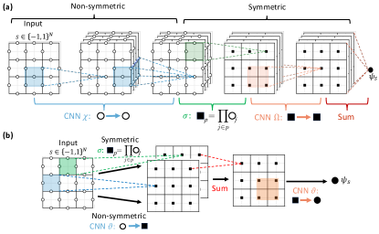
In this Letter, we demonstrate that approximately-invariant neural networks can impose a soft inductive bias on the ground-state search while maintaining the flexibility to capture complex quantum states (e.g. spin liquids) that are not exactly symmetric [Fig. 1(a)].
Our main results are threefold. First, to impose approximate symmetries on neural quantum states, we leverage techniques from the field of approximately group-equivariant networks [40, 41]. We modify these constructions for quantum many-body problems, incorporating physical insights into the structure of the neural network. Next, we demonstrate the accuracy of our approach on a paradigmatic quantum spin liquid model: the toric code perturbed by a magnetic field. We show that the variational energies obtained: (i) outperform conventional NQS methods; (ii) converge to exact diagonalization results for small system sizes [Fig. 2(b)]; (iii) match state-of-the-art tensor network and quantum Monte Carlo results for larger system sizes [Fig. 2(c)]; and (iv) enable access to large system sizes () even when the Hamiltonian has a significant sign problem, beyond the reach of both QMC and finite-size matrix product state methods [Fig. 1(c)]. Finally, we discuss how the approximate-symmetries framework facilitates NQS interpretability. In particular, we argue that the neural network discovers a representation of the emergent ground-state symmetries of spin liquids in the spirit of the quasi-adiabatic continuation of Hastings and Wen [Fig. 1(a)] [14].
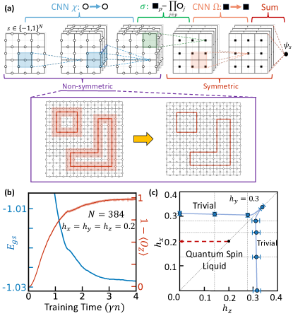
Emergent symmetries and the toric code—Consider an square lattice with open boundary conditions and qubits placed on its edges [Fig. 1(a)]. The mixed-field, toric-code model is given by the following Hamiltonian:
| (1) |
where , and are Pauli operators, the vertex operator acts on qubits neighboring a lattice vertex , and the plaquette operator acts on qubits around a square plaquette . Let us begin by considering the case where . In this regime, it is well-understood that the phase diagram hosts a gapped quantum spin liquid up to finite values of and [42, 43, 44]. Along the line, there is an exact local symmetry group, , generated by the operators. To wit, the ground state is invariant under , . We refer to elements of as loop operators, , since they have support on closed loops on the dual lattice.
For , exact symmetry under no longer holds. Nonetheless, as long as the system remains in the gapped spin liquid phase, it is possible to quasi-adiabatically continue the ground state back to the line, where is again exact [14]. Crucially, the continuation is accomplished by a local unitary, , which implies that for there are a set of “fattened” loop operators, , which remain symmetries of the ground state. The fattened loop operators are supported on ribbons of finite width about the unperturbed contours , up to exponentially small errors [Fig. 1(a)].
Approximate symmetries in neural networks—In order to exploit the emergent symmetries to improve the NQS ansatz, we must first construct an approximately-invariant neural network. For a system composed of qubits, each with state-space , a many-body quantum state vector can be decomposed into a complete basis labeled by bit strings : , where is a complex amplitude and is the quantum state associated with the bit string (e.g. ).
The key idea underlying NQS is to represent as a neural network that gives a complex scalar output for a particular bit string input, . To compute the ground state of a Hamiltonian, , one solves a variational energy-minimization problem with respect to the parameters, , of the neural network: . The energy is typically evaluated via Monte Carlo Markov chain sampling [22], while the network parameters are optimized via either gradient descent or more complicated second order methods (e.g. stochastic reconfiguration [45, 46, 47]).
Let us now consider the problem of incorporating approximate symmetries into an NQS ansatz. Suppose that the ground state, , exhibits a particular group of symmetries , such that for all . We will assume that the basis is chosen such that the group acts as a permutation on bit-string basis elements. In such a basis, the invariance of the state under is ensured if two inputs of the network connected by symmetry yield the same output (i.e. complex amplitude): for all [31, 34].
For approximate symmetries, the strict invariance condition above is relaxed to , where the expectation value is taken over all group elements and input bit strings [48]. Given a fully invariant neural network with , one can lift the strict constraints by adding an extra non-invariant layer to the network or by using a non-invariant skip-connection [41, 40]. In principle, for sufficiently large invariance breaking, , a neural network constructed in such a fashion can target any vector in the Hilbert space. In practice, the appropriate value of is learnt by the network itself, and is independent of network hyperparameters [13].
Approximately-invariant neural quantum states for the toric code—We propose a family of approximately-symmetric neural networks utilizing the so-called “combo” architecture [41, 13]. While we focus on the mixed field toric code model [Eqn. 1], our approach is applicable to a broad class of quantum spin liquid problems.
Our proposed architecture is schematically depicted in Fig. 2(a) and structured as follows: we first impose the constraints on the neural network and then weakly break these constraints by transforming the input with a non-invariant layer. More specifically, the neural network is defined by . Here, is the bit string input, is a non-invariant convolutional layer acting on the qubits and is a -invariant non-linearity which maps qubits to plaquettes. Finally, is a further convolutional layer (consisting of square-shaped kernels) acting on the plaquettes themselves followed by a summation and exponentiation to calculate [Fig. 2(a)]. The non-invariant convolutional layer has a kernel centered at each link of the lattice, and explicitly breaks the symmetry. Meanwhile, the non-linear layer, , is constructed using the -invariant operators, (since ) and ensures the -invariance of any further layers [36, 49]. We describe a number of other choices for approximately-symmetric architectures, along with their implementation details, in the Suppl. Mat. [13].
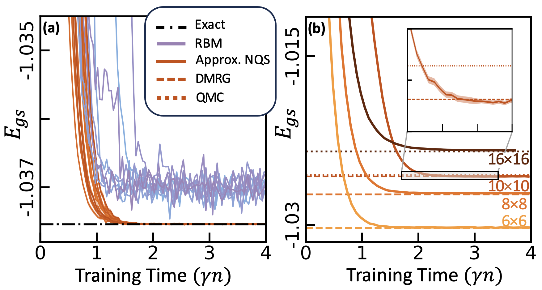
Let us begin benchmarking the accuracy of the approximately-symmetric NQS architecture for the mixed-field toric-code Hamiltonian in the sign-problem-free case (with and ). Starting with small lattices ( spins), we compute the ground state energy density, , using (i) our architecture; (ii) a conventional restricted Boltzmann machine (RBM), with lattice symmetries implemented; and (iii) exact diagonalization. The energy as a function of training time (measured in units of stochastic reconfiguration stepsize times iteration number ) is depicted in Fig. 2(b). While the RBM becomes stuck in local minima for all runs (with different initializations and hyperparameters) [22, 50], the approximately-symmetric architecture converges to the exact diagonalization energy with a relative error, .
We further find that the performance of the approximately-symmetric NQS is not limited to small values of the symmetry-violating field. Indeed, it is accurate to a relative error of even outside of the topological phase at [13]. This suggests that the ansatz is more widely applicable than naively expected and enables us to identify the phases and phase transitions out of the spin-liquid state within one NQS architecture.
To demonstrate the scalability of the architecture, we perform an extensive set of numerical simulations on lattices up to ( spins) using three methods: state-of-the-art DMRG (density matrix renormalization group) [51, 52, 53, 15], continuous-time QMC [42, 54, 55], and the approximately-symmetric NQS architecture. As illustrated in Fig. 2(c), the approximately-symmetric NQS yields competitive energies at all system sizes [inset, Fig. 2(c)]. Due to memory constraints, we were unable to obtain converged DMRG results for the lattice.
Toric code with a sign problem—Many physical perturbations naturally lead to sign problems, including magnetic fields, frustrated long-range couplings, and antiferromagnetic Heisenberg interactions [3, 56, 57]. In principle, variational methods such as DMRG can be used to study such models, even as QMC hits an exponential sampling barrier. However, as we have just seen in the sign-problem-free case, the memory requirements for DMRG on finite-size two-dimensional clusters can quickly become prohibitive. Accordingly, this is a regime in which the NQS approach should be uniquely well-suited.
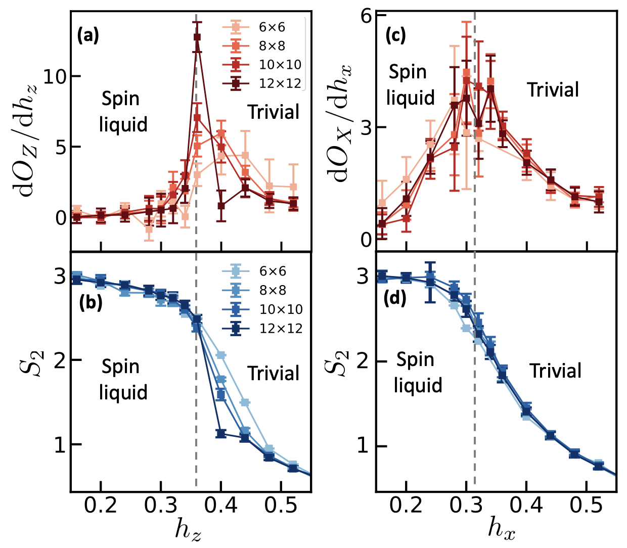
We introduce a sign problem in the toric code by turning on . We compute the ground state phase diagram as a function of and [Fig. 1(c)]. We utilize two diagnostics to identify the transition out of the spin liquid phase: (i) the string order parameter due to Bricmont, Frölich, Fredenhagen, and Marcu [58, 59] and (ii) the entanglement entropy.
The string order parameter, , diagnoses the confinement of the e-type excitations of the toric code. Consider a closed square loop of side length on the primal lattice. The order parameter is defined in the limit ,
| (2) |
where is the open string corresponding to half of the square . One expects to be finite in the trivial, confining, phase, while it vanishes in the spin liquid phase because each end of the open string creates a deconfined excitation [59, 58, 60]. An analogous order parameter, , diagnosing the confinement of m-type excitations, can be defined with strings on the dual lattice and Pauli operators. Our second diagnostic is the entanglement entropy, , where represents a particular subsystem. One expects the entanglement entropy to be larger deep in the spin liquid phase, since the trivial phase is smoothly connected to an unentangled product state.
As shown in Fig. 3, both of these expectations are borne out by the NQS simulations (at ). In particular, fixing and sweeping , we observe a pronounced peak in the derivative of the string order parameter, [Fig. 3(a)], as well as a sharp change in the entanglement entropy at the same field strength [Fig. 3(b)]. Analogous results fixing and sweeping are depicted in Figs. 3(c,d). To estimate the location of the thermodynamic critical point [Fig. 1(c)], we perform a power-law extrapolation in of the location of the observed finite-size cross-over [13]. After this finite-size extrapolation, the phase boundaries in [Fig. 1(c)] match those obtained by “infinite system-size” iPEPS and PCUT computations to about (Fig. 2 of [61, 62]).
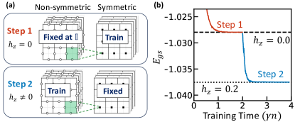
Interpretability—The approximately-symmetric NQS architecture facilitates partial interpretation of which physical features are learnt by different sections of the network. In particular, the non-invariant block maps the model from an approximately-symmetric regime to an exactly-symmetric one, which the -invariant block of the architecture can then learn efficiently. This mapping is analogous to the quasi-adiabatic continuation of Hastings and Wen [14], in which the exact “emergent” symmetries of the model (i.e. the “fattened” loops) are constructed by applying a finite-depth unitary circuit to the unperturbed toric code. We hypothesize that the dominant effect of the non-invariant block of the network is to reverse this finite-depth unitary dressing.
To test this hypothesis, we investigate the following two-step training scheme [Fig. 4(a]): First, we train the network in the fully symmetric regime at , by optimizing only the parameters of the invariant layer and keeping the non-invariant layer fixed to the identity. Second, we fix the invariant layer at these optimized parameters and turn on a field () which breaks the exact invariance of the state under the group, ; then, we find the ground state by only optimizing the parameters of the layer. Despite this restricted training procedure, we still obtain an excellent ground state energy [Fig. 4(b)], strongly suggesting that the network is indeed effectively learning the “fattened” loops [Fig. 1(a), red arrow] [13].
Outlook—Our work opens the door to a number of intriguing directions. First, by generalizing our approach to arbitrary groups [63, 64], it may be possible to apply the approximately-symmetric NQS framework to Dirac spin liquids or chiral spin liquids [65]. Second, on the numerical front, there are multiple avenues for further improvement, including: (i) tuning the depth of the architecture, (ii) exploring alternative representations for the complex amplitudes required for models with sign problems, (iii) increasing parameter efficiency with pooling layers, or (iv) replacing the CNNs with more elaborate backbone architectures (e.g. transformers) [26]. Finally, although our focus here is on the toric code spin liquid ground states, the approximately-symmetric architecture can be applied for any model with approximate symmetries, as well as real-time evolution problems.
Acknowledgements We gratefully thank DinhDuy Vu, Andrea Pizzi, Johannes Feldmeier, Quynh Nguyen, Rui Wang, Wen-Tao Xu, Marc Machaczek, Di Luo, Phil Crowley, Yichen Huang, Marc Finzi, Max Welling, Shivaji Sondhi, Saumya Shivam, Ruben Verresen, Robert Huang, Leo Lo, Joaquin Rodriguez-Nieva, Lode Pollet, Arthur Pesah for interesting discussions. We also thank Curtis McMullen for an inspiring group theory class. We acknowledge support from the NSF via the STAQ II program and the QLCI program (grant no. OMA-2016245), and from the Wellcome Leap under the Q for Bio program. D.K. acknowledges support from a Generation-Q AWS and HQI fellowship. S.M.L. acknowledges support from the European Research Council (ERC) under the European Union’s Horizon 2020 research and innovation program (Grant Agreement no 948141) from ERC Starting Grant SimUcQuam. N.Y.Y. acknowledges support from a Simons Investigator Award.
References
- Anderson [1973] P. W. Anderson, Resonating valence bonds: A new kind of insulator?, Materials Research Bulletin 8, 153 (1973).
- Kitaev [2006] A. Kitaev, Anyons in an exactly solved model and beyond, Annals of Physics 321, 2 (2006).
- Savary and Balents [2016] L. Savary and L. Balents, Quantum spin liquids: a review, Reports on Progress in Physics 80, 016502 (2016).
- Verresen et al. [2021] R. Verresen, M. D. Lukin, and A. Vishwanath, Prediction of toric code topological order from rydberg blockade, Physical Review X 11, 031005 (2021).
- Semeghini et al. [2021] G. Semeghini, H. Levine, A. Keesling, S. Ebadi, T. T. Wang, D. Bluvstein, R. Verresen, H. Pichler, M. Kalinowski, R. Samajdar, et al., Probing topological spin liquids on a programmable quantum simulator, Science 374, 1242 (2021).
- Satzinger et al. [2021] K. Satzinger, Y.-J. Liu, A. Smith, C. Knapp, M. Newman, C. Jones, Z. Chen, C. Quintana, X. Mi, A. Dunsworth, et al., Realizing topologically ordered states on a quantum processor, Science 374, 1237 (2021).
- Iqbal et al. [2024] M. Iqbal, N. Tantivasadakarn, R. Verresen, S. L. Campbell, J. M. Dreiling, C. Figgatt, J. P. Gaebler, J. Johansen, M. Mills, S. A. Moses, et al., Non-abelian topological order and anyons on a trapped-ion processor, Nature 626, 505 (2024).
- goo [2023] Non-abelian braiding of graph vertices in a superconducting processor, Nature 618, 264 (2023).
- Broholm et al. [2020] C. Broholm, R. J. Cava, S. A. Kivelson, D. G. Nocera, M. R. Norman, and T. Senthil, Quantum spin liquids, Science 367, eaay0668 (2020), https://www.science.org/doi/pdf/10.1126/science.aay0668 .
- Xu et al. [2023] S. Xu, R. Bag, N. E. Sherman, L. Yadav, A. I. Kolesnikov, A. A. Podlesnyak, J. E. Moore, and S. Haravifard, Realization of u (1) dirac quantum spin liquid in ybzn2gao5, arXiv preprint arXiv:2305.20040 (2023).
- Scheie et al. [2024] A. Scheie, E. Ghioldi, J. Xing, J. Paddison, N. Sherman, M. Dupont, L. Sanjeewa, S. Lee, A. Woods, D. Abernathy, et al., Proximate spin liquid and fractionalization in the triangular antiferromagnet kybse2, Nature Physics 20, 74 (2024).
- Zhang et al. [2024] Q. Zhang, W.-Y. He, Y. Zhang, Y. Chen, L. Jia, Y. Hou, H. Ji, H. Yang, T. Zhang, L. Liu, H.-J. Gao, T. A. Jung, and Y. Wang, Quantum spin liquid signatures in monolayer 1T-NbSe2, Nature Communications 15, 2336 (2024).
- [13] Please see the Supplementary Materials.
- Hastings and Wen [2005] M. B. Hastings and X.-G. Wen, Quasiadiabatic continuation of quantum states: The stability of topological ground-state degeneracy and emergent gauge invariance, Physical review b 72, 045141 (2005).
- Schollwöck [2011] U. Schollwöck, The density-matrix renormalization group in the age of matrix product states, Annals of Physics 326, 96 (2011), january 2011 Special Issue.
- Haegeman et al. [2011] J. Haegeman, J. I. Cirac, T. J. Osborne, I. Pižorn, H. Verschelde, and F. Verstraete, Time-dependent variational principle for quantum lattices, Physical review letters 107, 070601 (2011).
- Bañuls [2023] M. C. Bañuls, Tensor network algorithms: A route map, Annual Review of Condensed Matter Physics 14, 173 (2023).
- McMillan [1965] W. L. McMillan, Ground state of liquid , Phys. Rev. 138, A442 (1965).
- Ceperley et al. [1977] D. Ceperley, G. V. Chester, and M. H. Kalos, Monte carlo simulation of a many-fermion study, Phys. Rev. B 16, 3081 (1977).
- Kent et al. [1999] P. R. C. Kent, R. J. Needs, and G. Rajagopal, Monte carlo energy and variance-minimization techniques for optimizing many-body wave functions, Phys. Rev. B 59, 12344 (1999).
- Foulkes et al. [2001] W. M. C. Foulkes, L. Mitas, R. J. Needs, and G. Rajagopal, Quantum monte carlo simulations of solids, Rev. Mod. Phys. 73, 33 (2001).
- Carleo and Troyer [2017] G. Carleo and M. Troyer, Solving the quantum many-body problem with artificial neural networks, Science 355, 602 (2017).
- Hornik et al. [1989] K. Hornik, M. Stinchcombe, and H. White, Multilayer feedforward networks are universal approximators, Neural networks 2, 359 (1989).
- Sharir et al. [2022] O. Sharir, A. Shashua, and G. Carleo, Neural tensor contractions and the expressive power of deep neural quantum states, Physical Review B 106, 205136 (2022).
- Sharir et al. [2020] O. Sharir, Y. Levine, N. Wies, G. Carleo, and A. Shashua, Deep autoregressive models for the efficient variational simulation of many-body quantum systems, Physical review letters 124, 020503 (2020).
- Sprague and Czischek [2023] K. Sprague and S. Czischek, Variational monte carlo with large patched transformers, arXiv preprint arXiv:2306.03921 (2023).
- Patil [2023] P. Patil, Quantum monte carlo simulations in the restricted hilbert space of rydberg atom arrays, arXiv preprint arXiv:2309.00482 (2023).
- Viteritti et al. [2022] L. L. Viteritti, F. Ferrari, and F. Becca, Accuracy of restricted boltzmann machines for the one-dimensional heisenberg model, SciPost Physics 12, 166 (2022).
- Valenti et al. [2022] A. Valenti, E. Greplova, N. H. Lindner, and S. D. Huber, Correlation-enhanced neural networks as interpretable variational quantum states, Physical Review Research 4, L012010 (2022).
- Choo et al. [2019] K. Choo, T. Neupert, and G. Carleo, Two-dimensional frustrated j 1- j 2 model studied with neural network quantum states, Physical Review B 100, 125124 (2019).
- Roth et al. [2023] C. Roth, A. Szabó, and A. H. MacDonald, High-accuracy variational monte carlo for frustrated magnets with deep neural networks, Physical Review B 108, 054410 (2023).
- Chen et al. [2023] Z. Chen, L. Newhouse, E. Chen, D. Luo, and M. Soljačić, Autoregressive neural tensornet: Bridging neural networks and tensor networks for quantum many-body simulation, arXiv preprint arXiv:2304.01996 (2023).
- Zhang et al. [2022] K. Zhang, S. Lederer, K. Choo, T. Neupert, G. Carleo, and E.-A. Kim, Hamiltonian reconstruction as metric for variational studies, SciPost Physics 13, 063 (2022).
- Cohen and Welling [2016] T. Cohen and M. Welling, Group equivariant convolutional networks, in International conference on machine learning (PMLR, 2016) pp. 2990–2999.
- Reh et al. [2023] M. Reh, M. Schmitt, and M. Gärttner, Optimizing design choices for neural quantum states, Physical Review B 107, 195115 (2023).
- Luo et al. [2021] D. Luo, G. Carleo, B. K. Clark, and J. Stokes, Gauge equivariant neural networks for quantum lattice gauge theories, Physical review letters 127, 276402 (2021).
- Luo et al. [2022] D. Luo, S. Yuan, J. Stokes, and B. Clark, Gauge equivariant neural networks for 2+ 1d u (1) gauge theory simulations in hamiltonian formulation, in NeurIPS 2022 AI for Science: Progress and Promises (2022).
- Luo et al. [2023] D. Luo, Z. Chen, K. Hu, Z. Zhao, V. M. Hur, and B. K. Clark, Gauge-invariant and anyonic-symmetric autoregressive neural network for quantum lattice models, Physical Review Research 5, 013216 (2023).
- [39] Of course, for some spin liquids, there may not even be exactly solvable lattice models for which the exact symmetry operators are known.
- Finzi et al. [2021] M. Finzi, G. Benton, and A. G. Wilson, Residual pathway priors for soft equivariance constraints, Advances in Neural Information Processing Systems 34, 30037 (2021).
- Wang et al. [2022] R. Wang, R. Walters, and R. Yu, Approximately equivariant networks for imperfectly symmetric dynamics, in International Conference on Machine Learning (PMLR, 2022) pp. 23078–23091.
- Wu et al. [2012] F. Wu, Y. Deng, and N. Prokof’ev, Phase diagram of the toric code model in a parallel magnetic field, Physical Review B 85, 195104 (2012).
- Trebst et al. [2007] S. Trebst, P. Werner, M. Troyer, K. Shtengel, and C. Nayak, Breakdown of a topological phase: Quantum phase transition in a loop gas model with tension, Physical review letters 98, 070602 (2007).
- Fradkin and Shenker [1979] E. Fradkin and S. H. Shenker, Phase diagrams of lattice gauge theories with higgs fields, Phys. Rev. D 19, 3682 (1979).
- Sorella [1998] S. Sorella, Green function monte carlo with stochastic reconfiguration, Physical review letters 80, 4558 (1998).
- Amari [1998] S.-I. Amari, Natural gradient works efficiently in learning, Neural computation 10, 251 (1998).
- Stokes et al. [2020] J. Stokes, J. Izaac, N. Killoran, and G. Carleo, Quantum natural gradient, Quantum 4, 269 (2020).
- [48] Here the expectation is calculated with respect to the probability .
- Favoni et al. [2022] M. Favoni, A. Ipp, D. I. Müller, and D. Schuh, Lattice gauge equivariant convolutional neural networks, Physical Review Letters 128, 032003 (2022).
- Vicentini et al. [2022] F. Vicentini, D. Hofmann, A. Szabó, D. Wu, C. Roth, C. Giuliani, G. Pescia, J. Nys, V. Vargas-Calderón, N. Astrakhantsev, et al., Netket 3: machine learning toolbox for many-body quantum systems, SciPost Physics Codebases , 007 (2022).
- White [1992] S. R. White, Density matrix formulation for quantum renormalization groups, Phys. Rev. Lett. 69, 2863 (1992).
- White [1993] S. R. White, Density-matrix algorithms for quantum renormalization groups, Phys. Rev. B 48, 10345 (1993).
- Schollwöck [2005] U. Schollwöck, The density-matrix renormalization group, Rev. Mod. Phys. 77, 259 (2005).
- Linsel et al. [2024] S. M. Linsel, A. Bohrdt, L. Homeier, L. Pollet, and F. Grusdt, Percolation as a confinement order parameter in lattice gauge theories (2024), arXiv:2401.08770 [quant-ph] .
- Greitemann and Pollet [2018] J. Greitemann and L. Pollet, Lecture notes on diagrammatic monte carlo for the fröhlich polaron, SciPost Physics Lecture Notes , 002 (2018).
- Chaloupka et al. [2010] J. c. v. Chaloupka, G. Jackeli, and G. Khaliullin, Kitaev-heisenberg model on a honeycomb lattice: Possible exotic phases in iridium oxides , Phys. Rev. Lett. 105, 027204 (2010).
- Jiang et al. [2012] H.-C. Jiang, H. Yao, and L. Balents, Spin liquid ground state of the spin- square - heisenberg model, Phys. Rev. B 86, 024424 (2012).
- Bricmont and Frölich [1983] J. Bricmont and J. Frölich, An order parameter distinguishing between different phases of lattice gauge theories with matter fields, Physics Letters B 122, 73 (1983).
- Fredenhagen and Marcu [1983] K. Fredenhagen and M. Marcu, Charged states in 2 gauge theories, Communications in Mathematical Physics 92, 81 (1983).
- Gregor et al. [2011] K. Gregor, D. A. Huse, R. Moessner, and S. L. Sondhi, Diagnosing deconfinement and topological order, New Journal of Physics 13, 025009 (2011).
- Dusuel et al. [2011] S. Dusuel, M. Kamfor, R. Orús, K. P. Schmidt, and J. Vidal, Robustness of a perturbed topological phase, Physical review letters 106, 107203 (2011).
- [62] Note the factor of rescaling in the definition of magnetic fields between our work and [61].
- Diaconu and Worrall [2019] N. Diaconu and D. Worrall, Learning to convolve: A generalized weight-tying approach, in International Conference on Machine Learning (PMLR, 2019) pp. 1586–1595.
- Vieijra and Nys [2021] T. Vieijra and J. Nys, Many-body quantum states with exact conservation of non-abelian and lattice symmetries through variational monte carlo, Physical Review B 104, 045123 (2021).
- Glasser et al. [2018] I. Glasser, N. Pancotti, M. August, I. D. Rodriguez, and J. I. Cirac, Neural-network quantum states, string-bond states, and chiral topological states, Physical Review X 8, 011006 (2018).
Supplementary Information:
Approximately-symmetric neural networks for quantum spin liquids
Dominik S. Kufel*1,2, Jack Kemp*1,2, Simon M. Linsel 3,4, Chris R. Laumann5, Norman Y. Yao1,2
1Department of Physics, Harvard University, 17 Oxford St., MA 02138, USA
2Harvard Quantum Initiative, 60 Oxford St., MA 02138, USA
3Faculty of Physics, Arnold Sommerfeld Centre for Theoretical Physics (ASC),
Ludwig-Maximilians-Universität München, Theresienstr. 37, 80333 München, Germany
4Munich Center for Quantum Science and Technology (MCQST), Schellingstr. 4, 80799 München, Germany
5Department of Physics, Boston University, 590 Commonwealth Avenue, Boston, Massachusetts 02215, USA
I Neural quantum states and symmetries of many-body systems
In the main text, we discussed the concept of approximately-symmetric networks and illustrated an explicit example of an approximately-symmetric NQS. Here we discuss the general methodology for constructing approximately-invariant NQS architectures. We start by discussing different ways of imposing many-body system symmetries on neural networks, followed by highlighting connections between our approach and group-equivariant neural network research in the ML community. We detail an explicit example of a different approximately-invariant architecture from the “combo” architecture in the main text, based on an alternate approach in the ML literature known as “residual pathway priors” (RPP).
I.1 Overview of different ways of imposing NQS symmetries
Symmetries of many body states () might be imposed on a neural network in multiple ways. If the symmetries of the states are also symmetries of the Hamiltonian, then the approach perhaps most familiar to a physicist is that of mimicking imposing symmetries in the exact diagonalization (ED). As discussed in the main text, in NQS one decomposes an arbitrary state in a certain basis where is typically chosen to be an eigenbasis of the operators. Then a simple way of imposing Hamiltonian symmetries is to turn to the shared eigenbasis of the Hamiltonian and symmetry group . This approach works for an arbitrary group and has been demonstrated in NQS for e.g., Heisenberg symmetric model by [1]. Within such approach one rotates the basis while recalculating matrix elements of the Hamiltonian (in a new basis) and picks a symmetry sector (particular representation of the symmetry group) e.g., for by selecting a subset of input bit strings. This approach plays well together with the standard MCMC sampling of bit string configurations in NQS: one initializes the MCMC chain in the symmetry-consistent configuration and then applies a symmetry-preserving update rule. For instance for a symmetry (e.g., of a quantum model) one would only sample configurations with a total spin by initializing the chain accordingly and later using total spin conserving rule for its updates (e.g., one which only exchanges individual spins within the configuration). It should be noted that within this approach the architecture of the neural network does not need to be constrained in any way, yet requires many less parameters to achieve the same relative error in ground state energy (see Fig. 2 in Ref. [1]).
Alternatively, another commonly used approach to imposing symmetries is “post-symmetrization” [2, 3] where one averages the output of the unconstrained NQS over the symmetry group i.e. in the simplest form where are characters of a chosen representation of the symmetry group (where is abelian). This approach suffers from an extra computational overhead proportional to the size of the group, and thus becomes infeasible for gauge groups or continuous symmetry groups. Its success also heavily depends on the specific choice of the post-symmetrization method: see Ref. [3] for details.
Finally in the autoregressive NQS, another method is instead to simply enforce that the probability of sampling configurations violating the state symmetry constraints vanishes [4, 5, 6].
We note that, for all the above methods, it is not immediately clear how to generalize them to the approximate symmetries context. We therefore turn to a class of methods which put constraints on the neural-network architecture itself, and allow flexible inclusion of approximate symmetries: group-equivariant neural networks.
I.2 (Approximately) group-equivariant neural networks
Group-equivariance and group-invariance
Group-equivariant networks [7] are neural network architectures which by construction are equivariant under the action of a particular symmetry group. Group equivariance is one of the essential building blocks for the success of the accurate protein structure prediction with AlphaFold 2 architecture [8]. So far, in the NQS context, group-equivariant networks have mostly been applied within the context of imposing lattice symmetries [9]. Within this approach, one restricts the NQS to (by construction) fulfill a certain constraint: in our case i.e. that of group-invariance of the output. Here we assume that the group action maps bit strings to bit strings 111Extending the applicability of the method beyond bit string to bit string mapping is perhaps possible by proceeding along lines of Ref. [49] where one imposes + lattice symmetries within the constrained neural network architecture utilizing idea of an equivariant Clebsch-Gordan nets [50]..
The usual way of imposing group-invariance on a neural network is to ensure group-equivariance of each of its layers, , and non-linearities. Group-equivariance of each layer means that where is an -dimensional input vector space, is an -dimensional output space, and and are the input and output representations of the symmetry group . In other words, for a -equivariant neural network, transforming the input by a certain group element corresponds to transforming features by the same group element (though perhaps expressed in a different representation). The difference between “equivariance” and “invariance” is intuitively illustrated in the animation [11]. As one transforms (rotates) an input (image in the left panel) to the -equivariant neural network, features extracted by the neural network transform accordingly (i.e. rotate; see middle panel). In a -invariant neural network (see right panel), as one transforms the input (left panel), feature fields remain unchanged. In other words, rotational equivariance might be thought of as an invariance in a co-transforming (co-rotating) frame. The fact that generic neural network architectures are not -equivariant might be illustrated on the case of the convolutional neural networks (CNNs) for the case of e.g., rotation group symmetries. CNNs are by construction translationally equivariant but are not rotationally equivariant. For any equivariant network, a final layer with a scalar output can be used to promote the equivarance to invariance, because it can be chosen to transform under the trivial representation of the symmetry group.
Approximate invariance
Critically, generalizing the above approach to approximate symmetries is straightforward: instead of demanding we demand for some as discussed in the main text (and where we average over group elements in and bit strings ). We emphasize that is learnt by the network itself, perhaps with a help of initialization at the fully symmetric point .
For completeness, we mention that our approach to imposing approximate symmetries within NQS might be perhaps also extended to the framework of Ref. [12]. Therein one evaluates NQS only on “canonical” bit strings which ensures equivariance of the output (for any Abelian group). A “canonical” bit string is a fixed representative of each equivalence class under the group action. Although it is unclear how efficient evaluation of such cannonicalization would be for general Abelian (gauge) groups, we point out an interesting connection to the recent ML literature: [13]. Therein a related cannonicalization function is learnt efficiently by an equivariant neural network. It is thus potentially feasible that the above approximate-symmetries framework might be carried on to this context as well (akin to [14]) - we leave this direction for future work.
I.3 General construction for approximately-symmetric NQS
Exactly-symmetric architecture
Here we present a general approach for imposing group equivariance in quantum many-body physics problems, provided that group action maps bit strings to bit strings i.e. . Following [15], we construct group-equivariant / group-invariant layers of the network by using equivariant multi-layered perceptrons (EMLP). There, equivariance is achieved by appropriately restricting weights of the multi-layered perceptron architecture. In special cases, this approach reduces to other group-equivariant frameworks such as G-convolutional [7], G-steerable [16] or deep set [17] architectures. We note that G-convolutional networks cannot be directly applied to problems possessing gauge symmetry since their evaluation cost scales with the size of the group. G-steerable convolutions, on the other hand, require decomposition of the group of symmetries onto semidirect product of group of translations and some other group [18] - which does not seem to be feasible in our case and would require recomputation of irreducible representations for every new group.
Within the EMLP framework, we consider linear layers with dimensions , which are constructed by appropriately restricting weights of the otherwise fully-connected layer. Weight restriction is obtained from an efficient algorithm [15], which is feasible since the cost of imposing equivariance couples only to the size of the generating set of the group—at worst for the groups we consider.
Due to the non-regular hidden-layer representations, one needs to ensure that the activation functions are also equivariant (i.e. that . Instead of traditionally used gated/norm [19] non-linearities, we utilize other gauge-equivariant non-linearities derived from a physical model in mind i.e. we construct the non-linearity as where is a gauge-invariant function of the input to a layer (an example of for a lattice gauge theory is described in the main text). Finally, in the last layer one applies a gauge-invariant non-linearity constructed in a similar fashion by . Note that for large symmetry groups (such as gauge groups discussed in the main text), most general linear equivariant layers fulfilling the gauge constraint might be trivial, e.g., for the gauge group from the main text, if one considers -dimensional hidden layer vector space, a linear equivariant layer would simply be proportional to the identity.
Finally, we remark that gauge-invariant architectures discussed above might also in principle be used to find selected excited states of the fully symmetric model. For example, for a purely -perturbed toric code, the lowest lying excitations would correspond to the lowest energy states within the -anyon excitation sectors. In practice, this might be achieved by applying a local basis transformation for the Hamiltonian where e.g., would introduce e-anyon excitation to vertices belonging to the boundary of the link . This method of finding an excited state might be further combined with the orthogonalization-based approach used in Refs. [12, 20].
Approximately-symmetric architecture
Let us now discuss how to generalize to the case when the symmetries are only approximate. The basic idea behind any such generalization is to add non-invariant blocks to an otherwise symmetric architecture. We demonstrate this approach with two examples: the “Combo” architecture in the spirit of [21], discussed in the main text, and the residual pathway prior “RPP” architecture in the spirit of [22]. The RPP architecture is constructed to mimic the ResNet [23] skip-connection architecture. Apart from a gauge-invariant pathway, it also contains a non-invariant skip-connection which allows incorporation of non-symmetric features. In practice, for , we construct the skip connection with a non--equivariant convolutional layer which maps set of edges to plaquettes. Finally the two pathways (equivariant and non-equivariant) are summed together and post-processed with another convolutional layer acting on plaquettes (as for the ”Combo” architecture) – see Fig. S1(b) for ”RPP” as compared with ”Combo” in Fig. S1(a).
We have implemented and tested both architectures, and find both yield comparable performance (see details below). However, the “Combo” architecture has the advantage that we have some physical intuition about the action the non-invariant layer (see the interpretability sections of the main text and also below for more details), which is why we chose to focus on that architecture.
II Approximately-symmetric NQS performance study
In this section, we first detail the specific hyperparameters used within our simulations, as well as the Monte Carlo Markov chain update rule we use. Second, we discuss the performance and characteristics of the model for a toric code in and fields. We claim that increasing the depth of the network allows us to systematically improve the accuracy of the simulations. Third, we then discuss the performance of the model under a variety of perturbations, both with and without a sign problem, and identify its key architectural components. Fourth, we track the main issues for further improving the accuracy of the network predictions in different regimes, culminating in suggestions for future architecture improvements with increased parameter-efficiency and enhanced performance. Finally, we provide more details on observable evaluations and extracting phase transitions with NQS.
II.1 Simulation parameters
For the simulations in the main text, we consider neural networks with real bit string inputs, (i) complex parameters and outputs if the Hamiltonian has a sign problem () and (ii) real parameters, and scalar positive outputs if the Hamiltonian is sign-problem-free () (as then underlying Hamiltonian is stoquastic so by Perron-Frobenius theorem the coefficients of the eigenvector can be chosen real and non-negative in the chosen basis [24]).
We evaluate the energy through Monte Carlo Markov chain (MCMC) sampling. It is performed by noting that where and where the latter is evaluated exactly for each bit string (due to only non-zero matrix elements of the Hamiltonian). Then for samples one approximates where samples are found by applying a Metropolis-Hastings algorithm.
We use a custom sampling rule, closely related to the one used in [25], which involves flipping either a single spin per update step, or all the spins surrounding a single vertex. The intution for this update rules stems from the fact that in the ground state of the toric code, a single spin-flip creates (two) excitations, whereas a vertex-flip does not. Thus close to the toric code fixed point, a single-spin flip update would generically be expected to take a high-amplitude state to a low amplitude state, in contrast to a vertex-flip. Nevertheless, single-spin flips are still required for ergodicity. Given vertices and spins, on each update we choose to flip a vertex with probability or else flip a spin. For open boundary conditions, we neglect any verticies with spins on the boundary in this procedure (for periodic boundary conditions, a more complicated procedure is required, see [25]). We find that this vertex-spin update rule empirically yields a significant improvement in MCMC sample acceptance probabilities compared to only using single spin updates.
In order to benefit from GPU parallelization, as well as improving the ergodicity of exploring possibly multi-modal probability landscapes, we draw samples from independent MCMC chains processed in parallel. We apply updates between each collected sample in order to reduce the autocorrelations within each chain. Furthermore, we discard the first samples while the chain thermalizes passed its initial transient. We evaluate using samples per chain, so that the total number of samples is . The total number of updates which must be applied is thus .
We initialize the neural network parameters such that the neural network is fully-symmetric before training. This is achieved by initializing the weights of the non-invariant kernels to and utilizing the sigmoid non-linearity in the non-invariant layers, given for real inputs as and (shift and rescaling of the sigmoid to ensure that for identity initialization of the non-invariant block). For invariant layers we use ELU non-linearity [26]. For complex neural network parameters, we separately pass real and imaginary parts of the input to the non-linearity (non-invariant layer) and (invariant layer) e.g., for either non-linearity .
We optimize the network parameters using stochastic reconfiguration [27] with diagonal shift regularization. This might be thought as an imaginary time evolution for the states [28] and amounts to 1st order time evolution on a TDVP manifold, yielding linear equations of motion for the vectorized parameters : where is a force vector, is a learning rate, and is a quantum geometric tensor (see e.g., [29] for details). We solve this equation by performing a singular value decomposition on the matrix, which has complexity of [30]. We choose it over the conjugate gradients solver with complexity (where is a condition number of the matrix ), because we empirically observed that for the family of ground states of the system and architecture under consideration is very large ( eigenvalues span to orders of magnitude) which in practice yields rather unpredictable and slower runtimes. Furthermore, in order to stabilize the simulations we add a small shift to the diagonal of the matrix i.e., .
Parameters used for running simulations with the architecture presented in Fig. (1a) of the main text for are listed in the Table 1 below. All simulations are run in NetKet [31] that benefits from JAX[32] auto-differentiation and just-in-time compilation. We follow the convention in NetKet 3.10 such that in code neural network outputs represent a logarithm of an amplitude to facilitate calculations. All neural networks are coded in FLAX [33]. DMRG simulations were performed in iTensor [34, 35] and exact diagonalization in Dynamite [36]. Energy densities as used in the figures are defined as i.e. energy per stabilizer. Training time in all figures refers to the (where is iteration number, and , as above, is a learning rate).
| Parameter Type | Parameter | Value |
| Optimization parameters | Learning rate | 7e-3 |
| Diagonal shift | 5e-5 | |
| Architecture parameters | NIB: Channels & Depth | |
| NIB: Initialization | Identity | |
| NIB: Kernel Size | 3 | |
| NIB: Non-linearity | ||
| IB: Channels & Depth | ||
| IB: Initialization | Random Gaussian | |
| IB: Kernel Size | 15 | |
| IB: Non-linearity | ||
| Total | 11324 | |
| Sampling characteristics | ||
| (per chain) | ||
II.2 Performance in and fields for a system
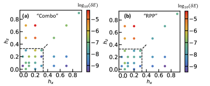
For a system and the “Combo” and “RPP” architectures, we plot the best relative error for different values of fields , optimized over hyperparameters after multiple simulation runs on a cluster (Fig. S2).
As expected from the built-in inductive bias, the neural network has the best performance for the small fields (where the approximate symmetries of the model are close to being exact). Although the network’s performance drops slightly as the value of the field is increased (owing to the increasing complexity of the wavefunction associated with the higher correlation length), the drop along the field is much more pronounced. As mentioned in the main text, the accuracy does not sharply diminish at the edge of the topological phase, but instead slowly decreases with the field, making the ansatz applicable even when is roughly comparable to the strength of the toric-code Hamiltonian coupling. Further, the energies obtained from our architecture (although not directly comparable due to different boundary conditions and system sizes) are much lower than these obtained in Ref. [20] when studied on the perturbed toric code model. Finally, we do not observe any significant differences in performance between the “RPP” and “Combo” architectures. We note that for systems, having a kernel size for the invariant part of the network covering the entire system () is crucial for achieving the reported accuracies (in contrast to the non-invariant network kernel size which can be without any significant loss in accuracy).
II.3 Performance under different perturbations for
We demonstrate that our ansatz is stable against a variety of different Hamiltonian perturbations: including ones introducing a sign problem. We broadly divide perturbations of the toric code Hamiltonian into different classes (see Table 2). For sign-problem-full perturbations, the Hamiltonian will not be stoquastic, and therefore the Frobenius theorem does not apply, permitting a non-trivial ground-state sign structure. For sign-problem-full perturbations we therefore allow for complex network outputs by using complex parameters.
| Perturbation type | Perturbation | |
|---|---|---|
| Sign-problem-free, invariant | XX | 1e-9 |
| Sign-problem-free, non-invariant | ZZ | 6e-8 |
| XX+YY+ZZ | 2e-5 | |
| XX+YY | 1e-5 | |
| Sign-problem-full, invariant | YYYY on plaquettes | 1e-5 |
| Sign-problem-full, non-invariant | Y | 1e-4 |
| YY | 1e-3 | |
| YYYY on vertices | 4e-6 |
We note that the performance of our ansatz has accuracy below for all perturbations tested. As generically expected [37], perturbations introducing sign-problem are more difficult for the NQS. This is most likely due to difficulty in propagation of complex phases through the network [38]. We notice that achieving the performance we have reached for the sign-problem-full case hinges upon including correlations between different channels of the non-invariant architecture as depicted in Fig. (1 a) of the main text. For instance, architecture with a ”bottleneck” where one sums over all channels before passing the output to the Wilson loop non-linearity, performs one to two orders of magnitude worse in accuracy as compared with the presented results.
Although we have not further tailored our ansatz for the sign-problem-full case, there are several ways of doing this e.g., by (i) experimenting with different complex phase representation e.g., by two decoupled networks with real parameters (one representing amplitude and the other the phase) [37, 39] and performing their sequential training [37, 39], (ii) modifying form of complex non-linearities within the complex parameters architectures [38].
II.4 Performance in magnetic fields for a system
Approximately-symmetric neural network analysis and improvement
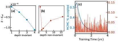
We proceed to investigating what limits the performance of the approximately-symmetric neural network. We first study the performance of the purely gauge-invariant architecture (constructed by omitting non-invariant block in the architecture in Fig. (2a) in the main text). We note that the relative energies (as compared with the state-of-the-art DMRG/QMC results) achieved for fields with a fully gauge-invariant architecture are comparable to these for with an approximately-symmetric one. We further observe a systematic scaling with the number of parameters and particularly depth of the network. We suggest therefore that the accuracy of the approximately-symmetric network behavior is not limited by the non-invariant block of the network but the invariant one. We investigate this hypothesis by investigating scaling of the relative energy error with the number of channels and depth of the symmetric and non-symmetric block of the network. In agreement with the purely gauge-invariant network results, we observe that by increasing the depth of the invariant part of the network, one can systematically improve the achievable energies (Fig. S3(a)). No similar scaling was observed with the depth of the non-invariant block (Fig. S3(b)) or the number of channels in the non-invariant or invariant part blocks (not shown). This conclusion holds for a range of other values of magnetic fields and system sizes.
We therefore suggest that the accuracy of our approximately-symmetric architecture might be improved by increasing the depth of the invariant part of the architecture. This might be potentially achieved by trying to further stabilize the training of deep neural network architectures (e.g., by introducing batch or layer normalization, see also [40]) and by increasing the efficiency of utilizing neural network parameters e.g., through pooling layers and decreasing invariant kernel sizes (simulations were run for -sized invariant kernels, but we did not observe any noticeable drop of accuracy in network performance with the reduction of the kernel size). Finally, one could try applying some of the transfer learning techniques [41] and optimizing ansatz with minSR for shorter runtimes [30]. We leave these suggested improvements for future work.
Sampling statistics
We provide more data on MCMC statistics for simulations on a system under an field to demonstrate that, for the system under consideration and architecture chosen, one does not run into any significant sampling issues. Sampling for the sign-problem full toric code with an field should be the most difficult: e.g., for stoquastic Hamiltonians it can be proven [42, 43] that MCMC mixing time for sampling their ground states scales polynomially with the number of qubits. To demonstrate that there are no issues with sampling, we show that (Fig. S3(c)): (i) the acceptance probabilities of the MCMC chain remain large () throughout the optimization; (ii) the energy autocorrelation time is small (where is ideal and one would like to avoid ). Furthermore, we verified that the split- characteristics [44] remains throughout the simulation (where is ideally and tolerance is heuristically recommended [44]).
II.5 Extracting phase transitions for a mixed field toric code
We provide more details about evaluating observables and extracting the phase diagram of the mixed field toric code under field (Fig. 1(c) main text). As mentioned in the main text, to find the phase transition we evaluate BFFM and observables ( and ) and second Renyi entropy. Assuming that observables of interests have only a polynomial number of non-zero matrix elements in each column of the matrix, they can be efficiently evaluated in the NQS by MCMC sampling [31]. This is indeed the case for the () order parameters (defined in the main text). Formally these observables become order parameters ( and ) only as the loop perimeter . In practice however, relatively small value of allows one to observe phase transitions. The intuition behind the () order parameters is the following: close to (unperturbed toric code limit) one would expect that the numerator is vanishing (open half-loop string creates two excitations at its ends which have a vanishing expectation value in a ground state) and denominator finite (closed Wilson loops are near exact symmetries of the ground state); away from point, closed Wilson loop decay exponentially with the loop perimeter , but this decay is compensated by a similar decay of the half-loops, leaving only the contributions from the endpoints yielding vanishing expectation value of the string order parameter [45].
On the other hand, the second Renyi entropy can be efficiently evaluated using Monte Carlo method as the expectation value of a SWAP operator on two copies of the state [46].
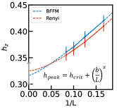
For a fixed cut through the phase diagram we find no significant shift of the peak in the derivative of both BFFM and second Renyi entropy with increasing which we associate with the location of the phase transition. For a fixed cut, on the other hand, we find stronger finite-size effects 222Lack of symmetry between and perturbations comes from the open boundary conditions: it might be seen in perturbation theory that and magnetic field excitations at the boundary give contributions to energy in different orders of perturbation theory. To obtain a more accurate estimate of the thermodynamic critical points along these cuts, we perform a simple finite-size extrapolation of the position of extracted and peaks (see Fig. S4). In particular, we fit the peak location to a power law in inverse system size, and extrapolate . Uncertainty in the extrapolation determines the uncertainty in critical point extraction (errorbars in Fig. 1(c) in the main text).
III Interpretability
We proceed to discussing interpretability of the approximately-symmetric neural network. We first discuss some caveats on the approximate-to-exact symmetries mapping proposed as the operational principle of the neural network. We second proceed to discuss the network invariance error (a quantity well-known in the machine-learning community [48]) and demonstrate that its derivative appears to exhibit divergent behavior at the same location as the phase transition from the quantum spin liquid to a trivial phase.
III.1 Approximate to exact symmetries mapping
In the main text we have argued that our approximately symmetric architecture operates mainly by mapping “fattened” Wilson loops to their known form at the fixed point within the non-symmetric block, and later solves the fully symmetric problem in the symmetric block. We have shown this strictly for an independent neural network training procedure (see main text). We expect this conclusion to largely hold for training both blocks together. One subtlety of the joint training is that the non-symmetric block is capable of learning some symmetric features of the state as well. One of the consequences of this is that after such training on (and ) simply setting weights of the non-invariant layer to an identity does not produce the ground state. We leave it for future investigations how to fully decouple features learnt by two blocks of the network during the joint training.
III.2 Invariance error
In the definition of the approximate group invariance , we defined a measure of the magnitude of the symmetry breaking, . Here we discuss the dynamics and asymptotic values of the closely related quantity as learnt by the neural network. We note that: (i) value of approaches the same value irrespective of the network hyperparameters over the course of optimization, (ii) appears to have a divergent derivative as one tunes the symmetry-violating field in a point closely matching the more conventional observables of the toric code phase transitions such as BFFM order parameters (see main text).
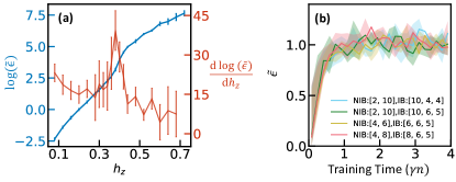
Invariance error universality
In the “Combo” approximately-symmetric architecture discussed in the main text, one increases the (maximum) degree of non-invariance implicitly by increasing the number of channels in the non-invariant layer. We note, however, that (and correspondingly ) converges to the same value towards the end of optimization (see Fig. S5b), regardless of the number of channel configuration (assuming that optimization has succeeded; this might require a certain minimum number of non-invariant channels).
Invariance error divergence
Furthermore, we found that the invariance error significantly increases with the increasing values of the field. To investigate this behaviour further we plot the as a function of field in the Fig. S5a. First, as expected, at the approximately-symmetric architecture learns to stay fully invariant (despite of extra flexibility). Second, we observe that reveals a peak matching the critical point found by more conventional observables (as in Fig. 3 main text). Such behavior is most likely comes from the connection of invariance error to the extent by which -Wilson loops act non-trivially on a system’s ground state: . It should be noted that, as expected, exhibits no such divergent behaviour when tuning symmetry-preserving terms (e.g., magnetic field) – under which the network stays fully invariant.
References
- Vieijra et al. [2020] Tom Vieijra, Corneel Casert, Jannes Nys, Wesley De Neve, Jutho Haegeman, Jan Ryckebusch, and Frank Verstraete, “Restricted boltzmann machines for quantum states with non-abelian or anyonic symmetries,” Physical review letters 124, 097201 (2020).
- Choo et al. [2019] Kenny Choo, Titus Neupert, and Giuseppe Carleo, “Two-dimensional frustrated j 1- j 2 model studied with neural network quantum states,” Physical Review B 100, 125124 (2019).
- Reh et al. [2023] Moritz Reh, Markus Schmitt, and Martin Gärttner, “Optimizing design choices for neural quantum states,” Physical Review B 107, 195115 (2023).
- Chen et al. [2023] Zhuo Chen, Laker Newhouse, Eddie Chen, Di Luo, and Marin Soljacic, “Antn: Bridging autoregressive neural networks and tensor networks for quantum many-body simulation,” Advances in Neural Information Processing Systems 36, 450–476 (2023).
- Luo et al. [2022] Di Luo, Shunyue Yuan, James Stokes, and Bryan Clark, “Gauge equivariant neural networks for 2+ 1d u (1) gauge theory simulations in hamiltonian formulation,” in NeurIPS 2022 AI for Science: Progress and Promises (2022).
- Hibat-Allah et al. [2020] Mohamed Hibat-Allah, Martin Ganahl, Lauren E Hayward, Roger G Melko, and Juan Carrasquilla, “Recurrent neural network wave functions,” Physical Review Research 2, 023358 (2020).
- Cohen and Welling [2016a] Taco Cohen and Max Welling, “Group equivariant convolutional networks,” in International conference on machine learning (PMLR, 2016) pp. 2990–2999.
- Jumper et al. [2021] John Jumper, Richard Evans, Alexander Pritzel, Tim Green, Michael Figurnov, Olaf Ronneberger, Kathryn Tunyasuvunakool, Russ Bates, Augustin Žídek, Anna Potapenko, et al., “Highly accurate protein structure prediction with alphafold,” Nature 596, 583–589 (2021).
- Roth et al. [2023] Christopher Roth, Attila Szabó, and Allan H MacDonald, “High-accuracy variational monte carlo for frustrated magnets with deep neural networks,” Physical Review B 108, 054410 (2023).
- Note [1] Extending the applicability of the method beyond bit string to bit string mapping is perhaps possible by proceeding along lines of Ref. [49] where one imposes + lattice symmetries within the constrained neural network architecture utilizing idea of an equivariant Clebsch-Gordan nets [50].
- [11] University of Amsterdam QUVA lab, “Group-equivariant neural network demonstration,” https://github.com/dom-kufel/g_equiv_networks/blob/main/conventional_cnn.gif.
- Choo et al. [2018] Kenny Choo, Giuseppe Carleo, Nicolas Regnault, and Titus Neupert, “Symmetries and many-body excitations with neural-network quantum states,” Physical review letters 121, 167204 (2018).
- Kaba et al. [2023] Sékou-Oumar Kaba, Arnab Kumar Mondal, Yan Zhang, Yoshua Bengio, and Siamak Ravanbakhsh, “Equivariance with learned canonicalization functions,” in International Conference on Machine Learning (PMLR, 2023) pp. 15546–15566.
- Kaba and Ravanbakhsh [2023] Sékou-Oumar Kaba and Siamak Ravanbakhsh, “Symmetry breaking and equivariant neural networks,” arXiv preprint arXiv:2312.09016 (2023).
- Finzi et al. [2021a] Marc Finzi, Max Welling, and Andrew Gordon Wilson, “A practical method for constructing equivariant multilayer perceptrons for arbitrary matrix groups,” in International conference on machine learning (PMLR, 2021) pp. 3318–3328.
- Cohen and Welling [2016b] Taco S Cohen and Max Welling, “Steerable cnns,” arXiv preprint arXiv:1612.08498 (2016b).
- Zaheer et al. [2017] Manzil Zaheer, Satwik Kottur, Siamak Ravanbakhsh, Barnabas Poczos, Russ R Salakhutdinov, and Alexander J Smola, “Deep sets,” Advances in neural information processing systems 30 (2017).
- Weiler and Cesa [2019] Maurice Weiler and Gabriele Cesa, “General e (2)-equivariant steerable cnns,” Advances in neural information processing systems 32 (2019).
- Weiler et al. [2018] Maurice Weiler, Mario Geiger, Max Welling, Wouter Boomsma, and Taco S Cohen, “3d steerable cnns: Learning rotationally equivariant features in volumetric data,” Advances in Neural Information Processing Systems 31 (2018).
- Valenti et al. [2022] Agnes Valenti, Eliska Greplova, Netanel H Lindner, and Sebastian D Huber, “Correlation-enhanced neural networks as interpretable variational quantum states,” Physical Review Research 4, L012010 (2022).
- Wang et al. [2022] Rui Wang, Robin Walters, and Rose Yu, “Approximately equivariant networks for imperfectly symmetric dynamics,” in International Conference on Machine Learning (PMLR, 2022) pp. 23078–23091.
- Finzi et al. [2021b] Marc Finzi, Gregory Benton, and Andrew G Wilson, “Residual pathway priors for soft equivariance constraints,” Advances in Neural Information Processing Systems 34, 30037–30049 (2021b).
- He et al. [2016] Kaiming He, Xiangyu Zhang, Shaoqing Ren, and Jian Sun, “Deep residual learning for image recognition,” in Proceedings of the IEEE conference on computer vision and pattern recognition (2016) pp. 770–778.
- Pillai et al. [2005] S Unnikrishna Pillai, Torsten Suel, and Seunghun Cha, “The perron-frobenius theorem: some of its applications,” IEEE Signal Processing Magazine 22, 62–75 (2005).
- Machaczek [2024] Marc Machaczek, “Neural quantum states for fracton models,” https://zenodo.org/records/10728168 (2024).
- Clevert et al. [2015] Djork-Arné Clevert, Thomas Unterthiner, and Sepp Hochreiter, “Fast and accurate deep network learning by exponential linear units (elus),” arXiv preprint arXiv:1511.07289 (2015).
- Sorella [1998] Sandro Sorella, “Green function monte carlo with stochastic reconfiguration,” Physical review letters 80, 4558 (1998).
- Stokes et al. [2020] James Stokes, Josh Izaac, Nathan Killoran, and Giuseppe Carleo, “Quantum natural gradient,” Quantum 4, 269 (2020).
- Carleo and Troyer [2017] Giuseppe Carleo and Matthias Troyer, “Solving the quantum many-body problem with artificial neural networks,” Science 355, 602–606 (2017).
- Chen and Heyl [2023] Ao Chen and Markus Heyl, “Efficient optimization of deep neural quantum states toward machine precision,” arXiv preprint arXiv:2302.01941 (2023).
- Vicentini et al. [2022] Filippo Vicentini, Damian Hofmann, Attila Szabó, Dian Wu, Christopher Roth, Clemens Giuliani, Gabriel Pescia, Jannes Nys, Vladimir Vargas-Calderón, Nikita Astrakhantsev, et al., “Netket 3: Machine learning toolbox for many-body quantum systems,” SciPost Physics Codebases , 007 (2022).
- Bradbury et al. [2018] James Bradbury, Roy Frostig, Peter Hawkins, Matthew James Johnson, Chris Leary, Dougal Maclaurin, George Necula, Adam Paszke, Jake VanderPlas, Skye Wanderman-Milne, and Qiao Zhang, “JAX: composable transformations of Python+NumPy programs,” (2018).
- Heek et al. [2023] Jonathan Heek, Anselm Levskaya, Avital Oliver, Marvin Ritter, Bertrand Rondepierre, Andreas Steiner, and Marc van Zee, “Flax: A neural network library and ecosystem for JAX,” (2023).
- Fishman et al. [2022a] Matthew Fishman, Steven R. White, and E. Miles Stoudenmire, “The ITensor Software Library for Tensor Network Calculations,” SciPost Phys. Codebases , 4 (2022a).
- Fishman et al. [2022b] Matthew Fishman, Steven R. White, and E. Miles Stoudenmire, “Codebase release 0.3 for ITensor,” SciPost Phys. Codebases , 4–r0.3 (2022b).
- Kahanamoku-Meyer and Wei [2024] Gregory D. Kahanamoku-Meyer and Julia Wei, “GregDMeyer/dynamite: v0.4.0,” (2024).
- Szabó and Castelnovo [2020] Attila Szabó and Claudio Castelnovo, “Neural network wave functions and the sign problem,” Physical Review Research 2, 033075 (2020).
- Jing et al. [2017] Li Jing, Yichen Shen, Tena Dubcek, John Peurifoy, Scott Skirlo, Yann LeCun, Max Tegmark, and Marin Soljačić, “Tunable efficient unitary neural networks (eunn) and their application to rnns,” in International Conference on Machine Learning (PMLR, 2017) pp. 1733–1741.
- Astrakhantsev et al. [2021] Nikita Astrakhantsev, Tom Westerhout, Apoorv Tiwari, Kenny Choo, Ao Chen, Mark H Fischer, Giuseppe Carleo, and Titus Neupert, “Broken-symmetry ground states of the heisenberg model on the pyrochlore lattice,” Physical Review X 11, 041021 (2021).
- Goodfellow et al. [2016] Ian Goodfellow, Yoshua Bengio, and Aaron Courville, Deep learning (MIT press, 2016).
- Zen et al. [2020] Remmy Zen, Long My, Ryan Tan, Frédéric Hébert, Mario Gattobigio, Christian Miniatura, Dario Poletti, and Stéphane Bressan, “Transfer learning for scalability of neural-network quantum states,” Physical Review E 101, 053301 (2020).
- Bravyi et al. [2022] Sergey Bravyi, David Gosset, and Yinchen Liu, “How to simulate quantum measurement without computing marginals,” Physical Review Letters 128, 220503 (2022).
- Bravyi et al. [2023] Sergey Bravyi, Giuseppe Carleo, David Gosset, and Yinchen Liu, “A rapidly mixing markov chain from any gapped quantum many-body system,” Quantum 7, 1173 (2023).
- Vehtari et al. [2021] Aki Vehtari, Andrew Gelman, Daniel Simpson, Bob Carpenter, and Paul-Christian Bürkner, “Rank-normalization, folding, and localization: An improved r for assessing convergence of mcmc (with discussion),” Bayesian analysis 16, 667–718 (2021).
- Xu et al. [2024] Wen-Tao Xu, Frank Pollmann, and Michael Knap, “Critical behavior of the fredenhagen-marcu order parameter at topological phase transitions,” arXiv preprint arXiv:2402.00127 (2024).
- Hastings et al. [2010] Matthew B Hastings, Iván González, Ann B Kallin, and Roger G Melko, “Measuring renyi entanglement entropy in quantum monte carlo simulations,” Physical review letters 104, 157201 (2010).
- Note [2] Lack of symmetry between and perturbations comes from the open boundary conditions: it might be seen in perturbation theory that and magnetic field excitations at the boundary give contributions to energy in different orders of perturbation theory.
- Finzi [2023] Marc Finzi, Understanding and Incorporating Mathematical Inductive Biases in Neural Networks, Ph.D. thesis, New York University (2023).
- Vieijra and Nys [2021] Tom Vieijra and Jannes Nys, “Many-body quantum states with exact conservation of non-abelian and lattice symmetries through variational monte carlo,” Physical Review B 104, 045123 (2021).
- Kondor et al. [2018] Risi Kondor, Zhen Lin, and Shubhendu Trivedi, “Clebsch–gordan nets: a fully fourier space spherical convolutional neural network,” Advances in Neural Information Processing Systems 31 (2018).