Emergent Gauge Fields in Band Insulators

Abstract

By explicit microscopic construction involving a mapping to a quantum vertex model subject to the ‘ice rule,’ we show that an electronically ‘trivial’ band insulator with suitable vibrational (phonon) degrees of freedom can host a “resonating valence-bond” state - a quantum phase with emergent gauge fields. This novel type of band insulator is identifiable by the existence of emergent gapless ‘photon’ modes and deconfined excitations, the latter of which carry non-quantized mobile charges. We suggest that such phases may exist in the quantum regimes of various nearly ferroelectric materials.

The term “resonating valence-bond (RVB) state,” initially introduced by Pauling in 1949 Pauling (1949), refers to phases of matter in which the quantum degrees of freedom fluctuate in a coherent way. The idea was revisited by Anderson Anderson (1973, 1987) in the context of frustrated quantum antiferromagnets, inspiring extensive theoretical investigations of “spin liquids” Savary and Balents (2016); Broholm et al. (2020); Zhou et al. (2017); Lee (2008) in “Mott insulators”, i.e. interaction dominated insulators with an odd number of electrons per unit cell, topological degeneracies (due to the Lieb-Schultz-Mattis theorem Lieb et al. (1961)), and fractionalized excitations Kivelson et al. (1987); Kalmeyer and Laughlin (1987). From a modern perspective, RVB belongs to the class of ‘topologically ordered’ quantum phases WEN (1990), whose universal properties have been mostly classified and characterized Wen (2017); Sachdev (2023).

Despite the successes of the abstract theory, it remains somewhat disappointing that while there are an increasing number of promising “spin liquid candidate materials,” Clark and Abdeldaim (2021); Chamorro et al. (2020); Trebst and Hickey (2022) there is no single solid material that has been indisputably established as having an RVB groundstate. Expanding the search for RVB to a broader range of systems is thus desirable, given that the essential feature of an RVB phase is the emergence of gauge fields at low energy Wen (1991, 1991); Read and Sachdev (1991); Senthil and Fisher (2000); Huse et al. (2003); Moessner and Sondhi (2003); Kitaev (2006); Moessner and Sondhi (2003); Fradkin et al. (2004); Vishwanath et al. (2004); Lee et al. (2006); Moessner et al. (2001); Levin and Wen (2003); Moessner and Raman (2010); Fradkin (2013); Sachdev (2016, 2018) which does not necessarily have any relation to spin physics and/or Mott insulators. Indeed, proposals for finding such topologically ordered states have been recently pursued in Rydberg atom arrays Semeghini et al. (2021); Verresen et al. (2021); Verresen and Vishwanath (2022); Samajdar et al. (2023).

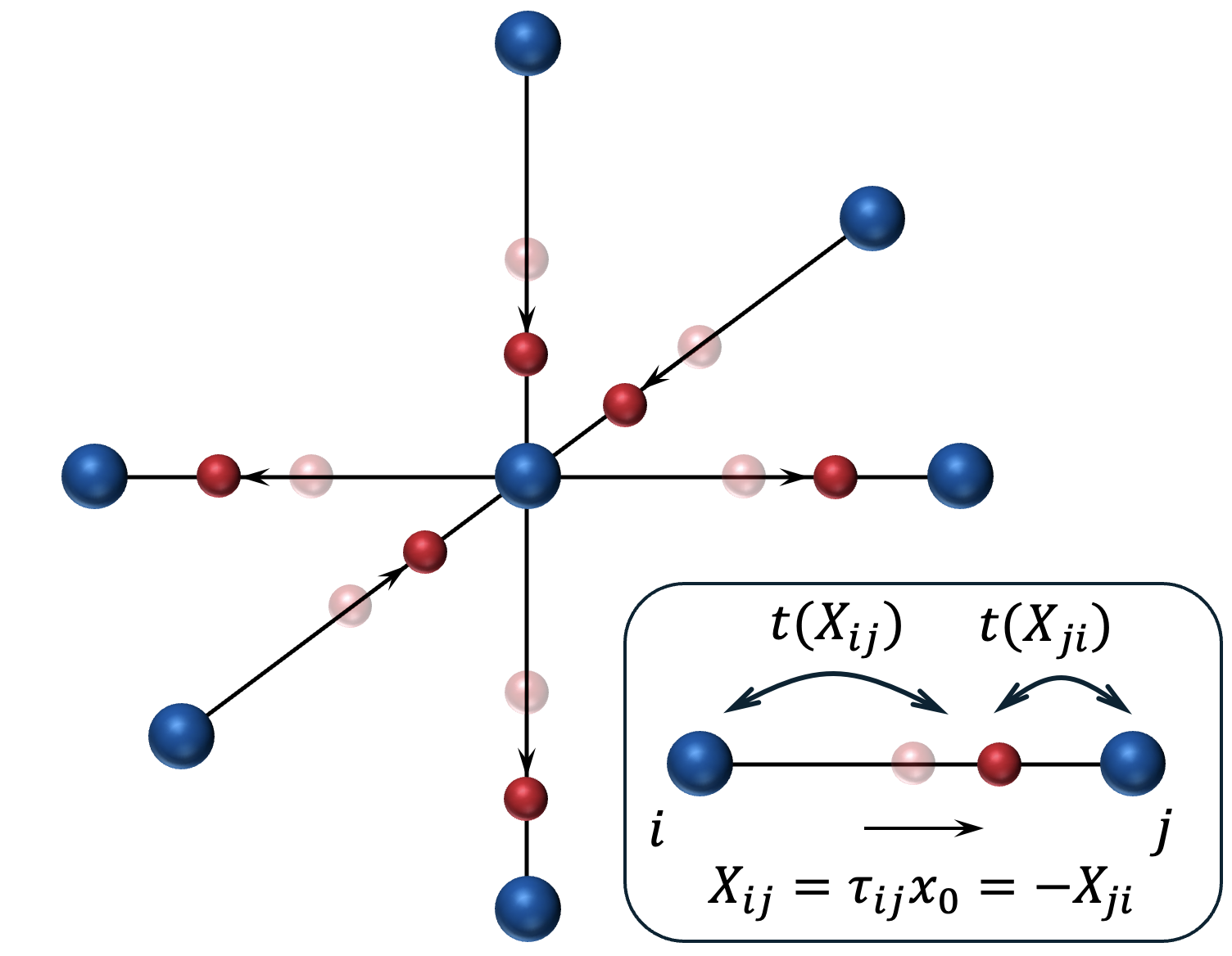
Figure 1: An illustration of the lattice structure around a lattice vertex and the ice-rule constraint: there are the same numbers of (red) bond atoms displaced toward as away from each (blue) vertex atom. Inset: the parametrization of a bond atom’s displacement and its effect on the electron hopping amplitude.

In this work, we articulate a different route to a quantum fluid phase with an emergent gauge field, which builds on phonon degrees of freedom on lattice bonds, roughly realizing the original intuitive picture of RVB. We note that certain aspects of this perspective have been discussed in studies of water ice Benton et al. (2016); Morris et al. (2019); Henley (2010); Gohlke et al. (2019); Lin et al. (2011); Chen et al. (1974); Benton et al. (2016); Castro Neto et al. (2006) and spin ice Knolle and Moessner (2019); Gingras and McClarty (2014); Castelnovo et al. (2012). To distinguish such states from the spin liquids discussed in much literature, we refer to them as phononic resonating-valence-bond (pRVB) states. Previously, we have shown with two explicit examples Han and Kivelson (2023); Cai et al. (2024) that certain models with strong electron-phonon couplings (EPC) and one electron per unit cell can exhibit RVB phases (i.e., Mott physics). Here, we consider the effect of another type of strong EPC in a band-insulator, where there is an even number of electrons per unit cell and always a gap in the electronic spectrum, even in the absence of EPC. We introduce an explicit minimal microscopic model (Eq. I) that captures the vibrational effects of atoms on lattice bonds, and show that when the strength of the EPC exceeds a certain threshold, the low-energy physics can be well described by a quantum vertex model whose Hilbert space is constrained by a (generalized) ice rule: around each lattice vertex, there are the same number of surrounding bond atoms that move closer to and away from it. (See Fig. 1 for illustrations.) This constraint is a highly non-perturbative consequence of the electrons’ effects on the phonons, as we establish using both exact arguments and numerical extensions. Then, by analyzing an exactly solvable point of the effective quantum vertex model and an effective field theory that is valid in the neighborhood of this point, we establish the possible existence of several phases in the phase diagram (see Fig. 2): a pRVB phase featuring an emergent $U(1)$ gauge field, a ferroelectric (FE) phase, and a phase with both FE order and an emergent gauge field that we refer to as FE^∗.

While our simple model does not directly apply to any specific material we know of, it is a plausible caricature of various nearly ferroelectric materials. We thus suggest that such materials should be reconsidered and reinvestigated in the context of “pRVB candidate materials.” To experimentally distinguish pRVB states from trivial band insulators, we analyze their identifying features, including the emergence of gapless transverse optical (TO) phonons and, at energy scales well below the electronic gap, deconfined excitations with a non-quantized charge. The latter should give rise to an anomalously high conductivity at temperatures well below the electronic gap.

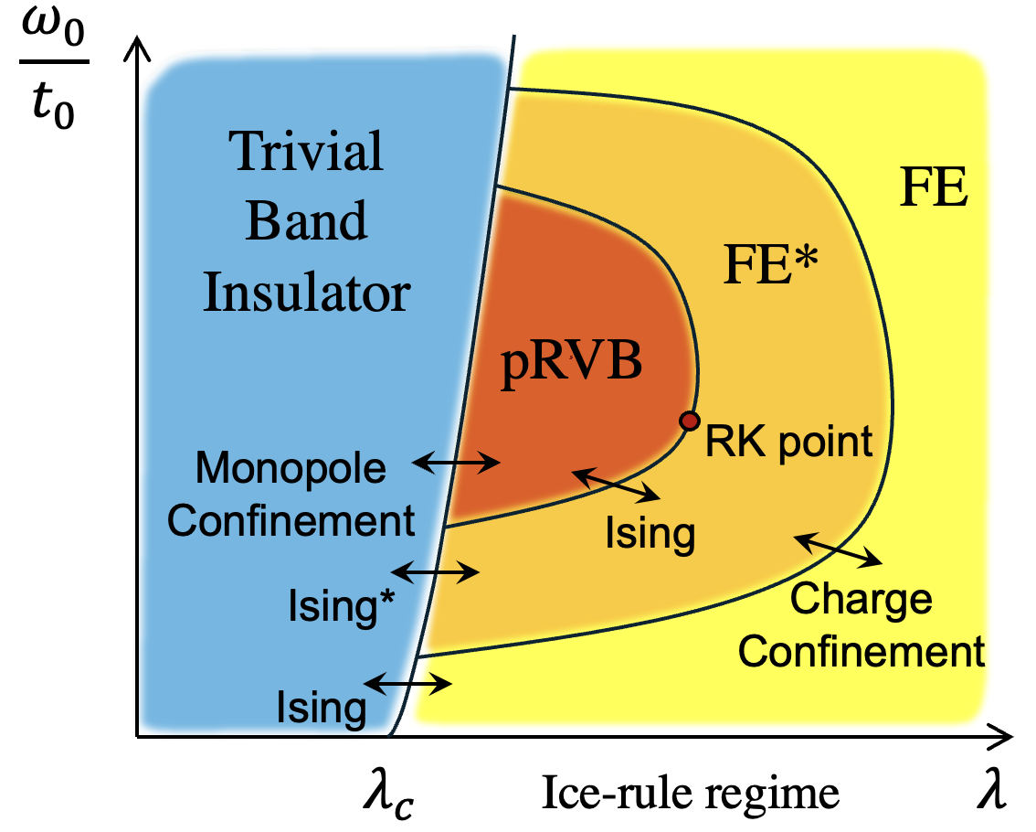
Figure 2: A schematic representation of one of the possible phase diagrams of the model in Eq. I. $\lambda=U_{\text{e-ph}}/t_{0}$ is a dimensionless measure of the strength of the EPC, i.e., the ratio between the EPC-induced interaction and the bare hopping amplitude. The nature of the various phases and phase transitions is discussed in the text.

I The microscopic model

We now introduce a model that captures the effects of the motion of bond-centered atoms parallel to the bonds’ direction. This model can be defined in any dimension on any lattice in which all the bonds are equivalent under the space group symmetry, and each bond perpendicularly intersects a (glide) reflection plane or a 180°-rotation axis at the bond center. This includes a huge family of lattices, e.g., simple, body-centered, or face-centered cubic, and diamond lattices in three dimensions. Given such a lattice, we consider its Lieb-type Lieb (2004) generalization by putting an extra atomic orbital on each bond center. The minimal model then reads:

$$\hat{H}= \sum_{i}\left[\Delta\ \hat{n}_{i}-\sum_{j\in\text{nn\ }i,\sigma}t(\hat{X}_{ij})\left(\hat{c}^{\dagger}_{i\sigma}\hat{f}_{\langle ij\rangle\sigma}+\text{h.c.}\right)\right]$$

$$\ \ \ +\sum_{\langle ij\rangle}\left(\frac{K\hat{X}_{ij}^{2}}{2}+\frac{\hat{P}_{ij}^{2}}{2M}\right)+\dots$$ (1)

where $\hat{c}_{i\sigma}$ and $\hat{f}_{\langle ij\rangle\sigma}$ are the electron annihilation operators on vertex $i$ and nearest-neighbor bond $\langle ij\rangle$, respectively, $\Delta$ is the charge transfer gap between vertex and bond orbitals, $\text{nn\ }i$ stands for the nearest neighboring vertices around vertex-$i$, and $\hat{X}_{ij}$ is the displacement of the bond atom relative to the center of bond $\langle ij\rangle$ in the direction of $i$-to-$j$ - i.e. $X_{ij}=-X_{ji}$ with the origin defined such that $X_{ij}=0$ when the bond atom is at the bond center. The phonons are assumed to be Einstein phonons with flat bare dispersion $\omega_{0}\equiv\sqrt{K/M}$, where $K$ is the bare stiffness, and $M$ is the bond atom mass. The symbol $\dots$ represents the additional physically plausible terms that we will first neglect and later treat perturbatively.

II The emergence of the ice rule

In the classical limit of the problem, where $M\rightarrow\infty$, the energy of the system is a function of the phonon configuration, $E^{\text{cl}}(\{X_{ij}\})$, which consists of the phonon elastic energy plus the sum of the electron energies in all occupied states - i.e. all states with energy below the Fermi level. This quantity is a complicated, non-local function of $\{X_{ij}\}$ for a general phonon configuration. However, as shown in Sec. I A of supplemental materials (SM), when the lattice coordination number is even, we prove a remarkable feature of the energy function:

Theorem I: For any electron density, $E^{\text{cl}}$ is the same for all phonon configurations in which the magnitudes of the atomic displacements are equal on all bonds, i.e., $|X_{ij}|=x_{0}$, and which satisfy an “ice rule” constraint at every vertex, i.e. $\sum_{j\in\text{nn }i}X_{ij}=0$.

We call these “ice-rule (satisfying) configurations” as this is a precisely realized version of the kind of (approximate) degeneracy of proton configurations seen in water ice. Any such $\{X_{ij}\}$ can be parameterized by the direction of polarization on each bond, i.e., $X_{ij}=\tau_{ij}x_{0}$ with $\tau_{ij}=-\tau_{ji}=\pm 1$ being oriented pseudospin variables, which in turn satisfy the constraints $\sum_{j\in\text{nn }i}\tau_{ij}=0$. The above theorem implies that, for ice-rule configurations, $E^{cl}$ generally depends on the amplitude $x_{0}$ but is independent of $\{\tau_{ij}\}$:

$$E^{\text{cl}}(\{X_{ij}\})=E^{\text{ice}}(x_{0}).$$ (2)

Addendum: Not only the classical ground-state energy but also the entire electronic spectra are exactly the same for all ice-rule configurations with the same $x_{0}$.

We emphasize the above statement is exact, regardless of the form of the function $t(x)$. This derives from the lattice symmetries we assumed and the special structure of the hopping matrix (i.e., there is no direct hopping between $f$ orbitals). Therefore, it not only holds for the specific Hamiltonian in Eq. I but pertains in the presence of various kinds of additional terms, such as direct hopping among $c$-orbitals, e.g. $\sum_{\langle ij\rangle}t^{\prime}(\hat{X}_{ij})(\hat{c}^{\dagger}_{i}\hat{c}_{j}+\text{h.c.})$, phonon coupling to the local electron densities, e.g. $\sum_{\langle ij\rangle}a(\hat{X}_{ij})(\hat{n}_{i}-\hat{n}_{j})+b(\hat{X}_{ij})(\hat{n}_{i}+\hat{n}_{j})+c(\hat{X}_{ij})\hat{n}_{\langle ij\rangle}$, etc.

We have not proven that ice-rule configurations are the global minima of $E^{\text{cl}}$, nor have we obtained an analytic expression for the optimal value of $x_{0}$ for them (although this is easy to determine numerically). However, we have proven a partial result:

Theorem II: For any electron density, ice-rule configurations are stationary points of the classical energy manifold with a fixed root-mean-square displacement.

To confirm whether such configurations are the classical ground states at electron densities corresponding to band insulators, we have numerically investigated the model on large clusters of various one-, two- and three-dimensional regular lattices with two electrons per vertex, adopting the simple form $t(x)=t_{0}-gx$, which is generic for small displacements (See Sec. I C of SM for results of the cubic lattice). We find that the ice-rule configurations (including the trivial case with $x_{0}=0$) are indeed always the lowest-energy ones at all sets of parameters we investigated; moreover, at generic values of the charge transfer gap $\Delta$, when the EPC-induced interaction strength $U_{\text{e-ph}}\equiv g^{2}/K$ surpasses a certain threshold determined by $t_{0}$ and $\Delta$, the system undergoes a continuous transition from a trivial band insulator (in which $E^{cl}$ is minimized by $x_{0}=0$) to an ice-rule regime with $x_{0}\neq 0$. Specifically, defining a dimensionless factor $\lambda\equiv U_{\text{e-ph}}/t_{0}$, we find that the optimal $x_{0}$ scales as $\sim\sqrt{\lambda-\lambda_{c}}$ as $\lambda$ approaches the critical value, $\lambda_{c}$, from the ice-rule regime. Meanwhile, the electronic spectrum is well-gapped on both sides of the transition with a gap $\sim|\Delta|$; thus, the system is always a ‘band insulator’ if only the electron sector of the problem is concerned.

III Effective Hamiltonian

Both the effects of non-infinite ion mass $M$ and other physically allowed couplings represented by $\dots$ in Eq. I generically lift the ice-rule degeneracy. So long as the additional interactions are weak (in appropriate units), their effects can be computed perturbatively. For example, dynamically induced degeneracy-lifting terms (which may cause “order by disorder”) can be computed in powers of $\omega_{0}$, starting with a leading term that encodes the configuration dependence of the zero-point energy of the phonons in the harmonic approximation. Moreover, non-zero $\omega_{0}$ also permits tunneling processes between distinct states in the degenerate ground-state manifold of $E^{cl}$; the amplitudes of such processes can be computed using semi-classical (instanton) methods. All these effects can be modeled by an effective Hamiltonian, $\hat{H}^{\text{eff}}$, that acts in the subspace of ice-rule configurations with basis states indexed by the direction of the dipole on each bond, $\{\tau_{ij}\}$. For the sake of concreteness, from here on, we focus on the case of a cubic lattice.

Since the leading order terms in $\hat{H}^{\text{eff}}$ are expected to be short-ranged, we focus our attention on the shortest-range terms consistent with the constraints of lattice symmetry and the ice rule. It is possible to express these as a sum of vertex terms - i.e., terms that operate on the bond variables radiating from a given vertex - and plaquette terms - i.e., those that depend on the bond variables surrounding an elementary plaquette. Fortunately, as shown in Sec. II B of SM, the ice-rule constraint makes the vertex terms redundant; the shortest-range model can thus be expressed entirely in terms of a sum over plaquette operators. The same analysis can be straightforwardly extended to other lattices and to include further neighbor interactions.

To most conveniently express the model, we pictorially represent the dipole variable $\tau_{ij}$ on each bond by an arrow and each square plaquette of the lattice by symbol . A given plaquette can have any of $2^{4}$ possible edge configurations, but these can be grouped into four equivalent types under the lattice symmetries, whose representatives are, respectively, type-$0$: , type-$1$: , type-$2$: , and type-$3$: . We denote the projector onto the subspace corresponding to type-$m$ configurations on a plaquette as $\hat{P}_{m}^{\kern 0.56001pt\leavevmode\hbox to4.67pt{\vbox to4.67pt{\text{[drawing]}}}\kern 0.56001pt}$. In terms of these, the effective model is

$$\hat{H}^{\text{eff}}=\sum_{\kern 0.56001pt\leavevmode\hbox to4.67pt{\vbox to4.67pt{\text{[drawing]}}}\kern 0.56001pt}\left[\sum_{m=1,2,3}V_{m}\hat{P}_{m}^{\kern 0.56001pt\leavevmode\hbox to4.67pt{\vbox to4.67pt{\text{[drawing]}}}\kern 0.56001pt}-J\left(\left|\kern 0.80002pt\leavevmode\hbox to14.63pt{\vbox to14.63pt{\text{[drawing]}}}\kern 0.80002pt\right\rangle\left\langle\kern 0.80002pt\leavevmode\hbox to14.63pt{\vbox to14.63pt{\text{[drawing]}}}\kern 0.80002pt\right|+\text{h.c.}\right)\right]$$

where $V_{m}$ terms are the interactions that are diagonal in the $\tau$ basis ($V_{0}$ is set to $0$ without loss of generality), and $J$ is the amplitude of the minimal quantum tunneling process within the ice-rule subspace activated by finite $\omega_{0}$. This is a variant of quantum vertex models discussed in Ref. Balasubramanian et al. (2022).

Because it derives from a tunneling process, $J\sim\mathrm{e}^{-S}$ where the tunneling action $S$ is proportion to $\sqrt{M}$, the tunneling distance $\sim x_{0}$, and the energy of the barrier to tunneling. Thus, whenever $\lambda$ is large enough to produce substantial dipolar displacements as well as tunneling barriers, $J$ is negligible compared to the interaction $V_{m}$’s. In this limit, $\hat{H}^{\text{eff}}$ is effectively classical ($J\approx 0$), with ordered ground states that can be determined exactly. Depending on the relative values of $\{V_{m}\}$, various phases are possible, including several distinct ferro-, antiferro- and ferri-electric orders, as we present in Sec. II C of SM.

However, as $\lambda$ approaches $\lambda_{c}$, the action of the minimal quantum tunneling event vanishes in proportion to $x_{0}^{3}\sim(\lambda-\lambda_{c})^{3/2}$ (Sec. I D of the SM). This derives from a combination of an increasingly small tunneling distance ($\sim x_{0}$) and an increasingly small tunnel barrier $\sim t_{0}x_{0}^{4}$. Thus, over a relatively broad range of circumstances not too far from criticality, where the magnitude of the dipolar distortions satisfies $(\lambda-\lambda_{c})^{3/2}\sim(\omega_{0}/t_{0})$, the model enters a highly quantum regime in which $J$ can be substantial and comparable to $V_{m}$.

IV Effective field theory

Fortunately, like its cousin - the quantum dimer model Rokhsar and Kivelson (1988) - this model has a so-called Rokhsar-Kivelson (RK) point at which the ground states are exactly solvable. This corresponds to $V_{3}=J$, $V_{1}=V_{2}=0$, where each groundstate is an equal superposition of all ice-rule configurations within a topological sector specified by the total ‘fluxes’ of $\tau_{ij}$ (viewing it as a vector field) through the non-contractible closed surfaces of the system. Also similar to the case in the quantum dimer model Moessner and Sondhi (2003); Fradkin et al. (2004); Moessner and Raman (2010); Fradkin (2013) in three dimensions, the long-wavelength physics near the RK point is described by a $U(1)$ gauge theory with Hamiltonian density (Sec. III A of SM):

$$\hat{\mathcal{H}}=\frac{1}{2\tilde{\epsilon}}|\hat{\bm{d}}|^{2}+\frac{1}{2\tilde{\mu}}\left(\kappa^{2}|\nabla\times\hat{\bm{d}}|^{2}+|\nabla\times\hat{\bm{a}}|^{2}\right)$$ (3)

where $\kappa$, $\tilde{\epsilon}$, $\tilde{\mu}$ are constants ($\kappa\approx 3.6$ for the cubic lattice), $\bm{d}$ is the coarse-grained field version of $\tau_{ij}/2$ subject to the ice-rule constraint $\nabla\cdot\bm{d}=0$, and $\hat{\bm{a}}$ is the conjugate field operator of $\hat{\bm{d}}$ that satisfies the canonical commutation relations $[\hat{\bm{d}}_{\alpha}(\bm{r}),\hat{\bm{a}}_{\beta}(\bm{r}^{\prime})]=\mathrm{i}\delta_{\alpha\beta}\delta(\bm{r}-\bm{r}^{\prime})$. By analogy to the electromagnetic (EM) field, $\bm{d}$ can be viewed as an emergent electric displacement field, and $\bm{b}\equiv\nabla\times\bm{a}$ is thus the emergent magnetic flux density. (The emergent electric and magnetic fields $\bm{e}\equiv\bm{d}/\tilde{\epsilon}$, $\bm{h}\equiv\bm{b}/\tilde{\mu}$ are related to these fields by the effective ‘permittivity,’ $\tilde{\epsilon}$, and ‘permeability,’ $\tilde{\mu}$.) At the RK point, the theory is anomalous in the sense that $1/\tilde{\epsilon}=0$. The corresponding field theory describes an unstable fixed point, obtained when the amplitude ($1/\tilde{\epsilon}$) of the only relevant operator ($\hat{\bm{d}}^{2}$) vanishes Fradkin et al. (2004).

Tuning away from this point, when $1/\tilde{\epsilon}>0$, the second term ($|\nabla\times\hat{\bm{d}}|^{2}$) can be dropped in the infrared limit, and the theory becomes exactly the same as that describing the usual EM gauge field. In this way, we have theoretically established the existence of the pRVB phase in the vicinity of the RK point of the model in Eq. III. Indeed, numerical studies on a similar vertex model on a diamond lattice have verified such a phase near its RK point Shannon et al. (2012); Pace et al. (2021); Sikora et al. (2011).

On the other hand, when $1/\tilde{\epsilon}<0$, higher-order terms need to be included, following which we find a variety of possible broken symmetry phases with finite expectation values of $\langle\bm{d}\rangle$ (See Sec. III B of SM for details). These higher terms are dangerously irrelevant perturbations of the unstable fixed point at $1/\tilde{\epsilon}=0$, which is thus a multicritical point. For instance, in the presence of positive quartic terms ($|\bm{d}|^{4}$ and $\sum_{\alpha=x,y,z}\bm{d}_{\alpha}^{4}$), the polarization does not jump discontinuously to large values but rather rises continuously with increasing $|1/\tilde{\epsilon}|$. The corresponding phase is a novel FE^∗ phase in which partial spontaneous polarization coexists with gapless emergent photons and deconfined excitations as in the $1/\tilde{\epsilon}>0$ phase. We sketch a possible phase diagram for this scenario in Fig. 2.

Like the native EM $U(1)$ gauge field, the emergent gauge field has gapless ‘photon’ excitations with ‘speed of light’ $\tilde{c}=1/\sqrt{\tilde{\epsilon}\tilde{\mu}}$, and couple to ‘charged’ excitations. Microscopically, the gapless photons are TO phonon modes. The elementary charged excitation is a local violation of the ice rule around a vertex that has a net $\pm 1$ units of electric flux, i.e. $\oint d\bm{S}\cdot\bm{d}=\pm 1$ for any surface enclosing it. Moreover, since this is an emergent gauge field on a lattice, magnetic monopole excitations are also possible, and they are quantized due to Dirac’s quantization. Both types of excitations are deconfined in the sense that two charges or monopoles interact at large distances via a Coulomb interaction. The transitions out of this deconfined Coulomb phase for the gauge theory can be understood as condensation of either the charges or the monopoles, which leads to the confinement of the other Fradkin and Shenker (1979); Fradkin (2013). By tracking the fate of the excitations at the phase boundaries, we are able to deduce the nature of the transitions in Fig. 2 (see Sec. IV of SM for details). In particular, the transition between the pRVB and trivial band insulator phases may be understood as condensation of the charge excitations, whose creation energy vanishes as $(\lambda-\lambda_{c})^{2}$ near the transition.

V Phenomenology of the pRVB phase

If one is lucky enough to find a material with a pRVB or FE* ground state, this can be established in several ways. In the first place, in addition to the usual acoustic modes, there should additionally exist two gapless TO phonon modes that are the ‘photons’ of the emergent $U(1)$ gauge fields. The speed of sound for these modes vanishes upon approaching any continuous phase boundary to an FE-ordered phase. Moreover, deconfined charge excitations corresponding to local violations of the ice rule have creation energy (gap) associated with the energy scale of the ice rule, which is generally much smaller than the electronic gap scale $\sim|\Delta|$ and vanishes upon approaching a continuous transition to the trivial band-insulator phase. These particles have an integer charge with respect to the emergent gauge fields, but an irrational charge, which is a continuous function of $(\lambda-\lambda_{c})$, under the EM field . Gapped emergent monopoles should also exist and similarly carry irrational magnetic charges (Sec. III B of SM.)

It is also useful to consider identifying features of materials that are somehow ‘close’ to realizing these phases. It would then be sensible to see if various relatively benign perturbations, such as applied pressure or strain, chemical doping, or isotopic substitution, can coax the system across a proximate phase boundary into a topological phase.

A trivial insulator close to an ice-rule regime can be expected to exhibit several characteristic features. Most obviously, as a herald of the emergence of the ice rule, it could exhibit a large susceptibility to all forms of ferroelectric orders that preserve the ice rule, indicative of strong collective local quantum fluctuations of dipolar modes. The other side of the same coin is that the corresponding phonon modes (including the TO modes) should become increasingly weakly dispersive and simultaneously soften at all momenta as $\lambda$ approaches $\lambda_{c}^{-}$ (Sec. I B&C of SM).

For a material within the ice-rule regime, then at temperatures large compared to all the terms that appear in $\hat{H}^{\text{eff}}$ but low compared to the energy scale enforcing the ice rule (if such a separation of scales exists), several observable properties can be probed that would indicate the emergence of the ice rule in the patterns of local dipolar distortions. It is well known that the ice rule implies a certain value of residual entropy that depends on the lattice structure (Sec. I A of SM). This also results in the existence of “pinch point(s)” in correlation functions of the bond dipoles Benton et al. (2016); Gohlke et al. (2019); Morris et al. (2019); Henley (2010).

Since the quantum term ($J$) essential to any pRVB physics involves the quantum tunneling of ions, one would expect that it will typically be small compared to the potential terms ($V_{m}$). This has two consequences for $\lambda>\lambda_{c}$: Firstly, it means that the equilibrium state at low $T$ is likely to be one of the topologically trivial broken symmetry states we have mentioned - for instance, a ferroelectric state. Secondly, all dynamical properties of the dipolar degrees of freedom will be slow, meaning that non-equilibrium states (such as those generic in water ice) may be unavoidable. However, recasting the tunnel action already discussed in a form that is expressed in terms of typical physical parameters, we see that $S\sim z\sqrt{M/m}\ (x_{0}/a_{B})^{3}$, where $z$ is the number of atoms involved in the resonance ($z=4$ for a square plaquette), $m$ is the electron mass and $a_{B}$ is the Bohr radius. For a typical value of $\sqrt{M/m}\sim 40-600$, this means that $J\sim e^{-S}$ is negligibly small whenever $x_{0}/a_{B}$ is order $1$. However, if through a clever intervention, one can access a regime in which $x_{0}/a_{B}$ of order $0.1$ or less, the quantum dynamical terms in $H^{\text{eff}}$ could be comparable to the potential terms. Thus, a “trivial” ferroelectric might be transformable into an FE* or a pRVB. It is also worth noting that more microscopically “realistic” versions of related EPC models can be explored numerically as they are free from the fermion-minus-sign problem Li and Yao (2019); Cai et al. (2024) and thus may be investigated using quantum Monte Carlo approaches with considerable fidelity (Sec. VI of SM).

Acknowledgement. We thank Shivaji Sondhi, Chaitanya Murthy, Vladimir Calvera, Ashvin Vishwanath, Zhi-Qiang Gao, Tibor Rakovszky, Jonah Herzog-Arbeitman, Fiona Burnell, Roderich Moessner, Chris Laumann, and Eduardo Fradkin for helpful communications. The work was funded, in part, by the Department of Energy, Office of Basic Energy Sciences, under Contract No. DE-AC02-76SF00515 at Stanford.

References

- Pauling (1949) L. C. Pauling, Proceedings of the Royal Society of London. Series A. Mathematical and Physical Sciences 196, 343 (1949), https://royalsocietypublishing.org/doi/pdf/10.1098/rspa.1949.0032 .
- Anderson (1973) P. Anderson, Materials Research Bulletin 8, 153 (1973).
- Anderson (1987) P. W. Anderson, Science 235, 1196 (1987), https://www.science.org/doi/pdf/10.1126/science.235.4793.1196 .
- Savary and Balents (2016) L. Savary and L. Balents, Reports on Progress in Physics 80, 016502 (2016).
- Broholm et al. (2020) C. Broholm, R. J. Cava, S. A. Kivelson, D. G. Nocera, M. R. Norman, and T. Senthil, Science 367, eaay0668 (2020), https://www.science.org/doi/pdf/10.1126/science.aay0668 .
- Zhou et al. (2017) Y. Zhou, K. Kanoda, and T.-K. Ng, Rev. Mod. Phys. 89, 025003 (2017).
- Lee (2008) P. A. Lee, Science 321, 1306 (2008), https://www.science.org/doi/pdf/10.1126/science.1163196 .
- Lieb et al. (1961) E. Lieb, T. Schultz, and D. Mattis, Annals of Physics 16, 407 (1961).
- Kivelson et al. (1987) S. A. Kivelson, D. S. Rokhsar, and J. P. Sethna, Phys. Rev. B 35, 8865 (1987).
- Kalmeyer and Laughlin (1987) V. Kalmeyer and R. B. Laughlin, Phys. Rev. Lett. 59, 2095 (1987).
- WEN (1990) X. G. WEN, International Journal of Modern Physics B 04, 239 (1990), https://doi.org/10.1142/S0217979290000139 .
- Wen (2017) X.-G. Wen, Rev. Mod. Phys. 89, 041004 (2017).
- Sachdev (2023) S. Sachdev, Quantum Phases of Matter (Cambridge University Press, 2023).
- Clark and Abdeldaim (2021) L. Clark and A. H. Abdeldaim, Annual Review of Materials Research 51, 495 (2021).
- Chamorro et al. (2020) J. R. Chamorro, T. M. McQueen, and T. T. Tran, Chemical Reviews 121, 2898 (2020).
- Trebst and Hickey (2022) S. Trebst and C. Hickey, Physics Reports 950, 1 (2022), kitaev materials.
- Wen (1991) X. G. Wen, Phys. Rev. B 44, 2664 (1991).
- Read and Sachdev (1991) N. Read and S. Sachdev, Phys. Rev. Lett. 66, 1773 (1991).
- Senthil and Fisher (2000) T. Senthil and M. P. A. Fisher, Phys. Rev. B 62, 7850 (2000).
- Huse et al. (2003) D. A. Huse, W. Krauth, R. Moessner, and S. L. Sondhi, Phys. Rev. Lett. 91, 167004 (2003).
- Moessner and Sondhi (2003) R. Moessner and S. L. Sondhi, Phys. Rev. B 68, 184512 (2003).
- Kitaev (2006) A. Kitaev, Annals of Physics 321, 2 (2006), january Special Issue.
- Fradkin et al. (2004) E. Fradkin, D. A. Huse, R. Moessner, V. Oganesyan, and S. L. Sondhi, Phys. Rev. B 69, 224415 (2004).
- Vishwanath et al. (2004) A. Vishwanath, L. Balents, and T. Senthil, Phys. Rev. B 69, 224416 (2004).
- Lee et al. (2006) P. A. Lee, N. Nagaosa, and X.-G. Wen, Rev. Mod. Phys. 78, 17 (2006).
- Moessner et al. (2001) R. Moessner, S. L. Sondhi, and E. Fradkin, Phys. Rev. B 65, 024504 (2001).
- Levin and Wen (2003) M. Levin and X.-G. Wen, Phys. Rev. B 67, 245316 (2003).
- Moessner and Raman (2010) R. Moessner and K. S. Raman, in Introduction to frustrated magnetism: materials, experiments, theory (Springer, 2010) pp. 437–479.
- Fradkin (2013) E. Fradkin, Field theories of condensed matter physics (Cambridge University Press, 2013).
- Sachdev (2016) S. Sachdev, Philosophical Transactions of the Royal Society A: Mathematical, Physical and Engineering Sciences 374, 20150248 (2016).
- Sachdev (2018) S. Sachdev, Reports on Progress in Physics 82, 014001 (2018).
- Semeghini et al. (2021) G. Semeghini, H. Levine, A. Keesling, S. Ebadi, T. T. Wang, D. Bluvstein, R. Verresen, H. Pichler, M. Kalinowski, R. Samajdar, A. Omran, S. Sachdev, A. Vishwanath, M. Greiner, V. Vuletić, and M. D. Lukin, Science 374, 1242 (2021), https://www.science.org/doi/pdf/10.1126/science.abi8794 .
- Verresen et al. (2021) R. Verresen, M. D. Lukin, and A. Vishwanath, Phys. Rev. X 11, 031005 (2021).
- Verresen and Vishwanath (2022) R. Verresen and A. Vishwanath, Phys. Rev. X 12, 041029 (2022).
- Samajdar et al. (2023) R. Samajdar, D. G. Joshi, Y. Teng, and S. Sachdev, Phys. Rev. Lett. 130, 043601 (2023).
- Benton et al. (2016) O. Benton, O. Sikora, and N. Shannon, Phys. Rev. B 93, 125143 (2016).
- Morris et al. (2019) D. J. P. Morris, K. Siemensmeyer, J.-U. Hoffmann, B. Klemke, I. Glavatskyi, K. Seiffert, D. A. Tennant, S. V. Isakov, S. L. Sondhi, and R. Moessner, Phys. Rev. B 99, 174111 (2019).
- Henley (2010) C. L. Henley, Annu. Rev. Condens. Matter Phys. 1, 179 (2010).
- Gohlke et al. (2019) M. Gohlke, R. Moessner, and F. Pollmann, Phys. Rev. B 100, 014206 (2019).
- Lin et al. (2011) L. Lin, J. A. Morrone, and R. Car, Journal of Statistical Physics 145, 365 (2011).
- Chen et al. (1974) M. Chen, L. Onsager, J. Bonner, and J. Nagle, The Journal of Chemical Physics 60, 405 (1974), https://pubs.aip.org/aip/jcp/article-pdf/60/2/405/18889204/405_1_online.pdf .
- Castro Neto et al. (2006) A. H. Castro Neto, P. Pujol, and E. Fradkin, Phys. Rev. B 74, 024302 (2006).
- Knolle and Moessner (2019) J. Knolle and R. Moessner, Annual Review of Condensed Matter Physics 10, 451 (2019), https://doi.org/10.1146/annurev-conmatphys-031218-013401 .
- Gingras and McClarty (2014) M. J. P. Gingras and P. A. McClarty, Reports on Progress in Physics 77, 056501 (2014).
- Castelnovo et al. (2012) C. Castelnovo, R. Moessner, and S. L. Sondhi, Annu. Rev. Condens. Matter Phys. 3, 35 (2012).
- Han and Kivelson (2023) Z. Han and S. A. Kivelson, Phys. Rev. Lett. 130, 186404 (2023).
- Cai et al. (2024) X. Cai, Z. Han, Z.-X. Li, S. A. Kivelson, and H. Yao, manuscript in preparation (2024).
- Lieb (2004) E. H. Lieb, Condensed Matter Physics and Exactly Soluble Models: Selecta of Elliott H. Lieb , 473 (2004).
- Balasubramanian et al. (2022) S. Balasubramanian, D. Bulmash, V. Galitski, and A. Vishwanath, arXiv preprint arXiv:2201.08856 (2022).
- Rokhsar and Kivelson (1988) D. S. Rokhsar and S. A. Kivelson, Phys. Rev. Lett. 61, 2376 (1988).
- Shannon et al. (2012) N. Shannon, O. Sikora, F. Pollmann, K. Penc, and P. Fulde, Phys. Rev. Lett. 108, 067204 (2012).
- Pace et al. (2021) S. D. Pace, S. C. Morampudi, R. Moessner, and C. R. Laumann, Phys. Rev. Lett. 127, 117205 (2021).
- Sikora et al. (2011) O. Sikora, N. Shannon, F. Pollmann, K. Penc, and P. Fulde, Phys. Rev. B 84, 115129 (2011).
- Fradkin and Shenker (1979) E. Fradkin and S. H. Shenker, Phys. Rev. D 19, 3682 (1979).
- Note (1) In the one-dimensional context, such irrationally charged soliton excitations were investigated theoretically in the classical () limit Rice and Mele (1982); Jackiw and Semenoff (1983); Kivelson (1983)and more recently in the presence of quantum effects using density-matrix-renormalization group methods Zhao and Kivelson (2024). That the defects in water ice may carry irrational charge has been noted in Ref. Moessner and Sondhi (2010); Morris et al. (2019).
- Li and Yao (2019) Z.-X. Li and H. Yao, Annual Review of Condensed Matter Physics 10, 337 (2019).
- Rice and Mele (1982) M. J. Rice and E. J. Mele, Phys. Rev. Lett. 49, 1455 (1982).
- Jackiw and Semenoff (1983) R. Jackiw and G. Semenoff, Phys. Rev. Lett. 50, 439 (1983).
- Kivelson (1983) S. Kivelson, Phys. Rev. B 28, 2653 (1983).
- Zhao and Kivelson (2024) S. Zhao and S. Kivelson, manuscript in preparation (2024).
- Moessner and Sondhi (2010) R. Moessner and S. L. Sondhi, Phys. Rev. Lett. 105, 166401 (2010).