Evolutive Rendering Models

Abstract.

The landscape of computer graphics has undergone significant transformations with the recent advances of differentiable rendering models. These rendering models often rely on heuristic designs that may not fully align with the final rendering objectives. We address this gap by pioneering evolutive rendering models, a methodology where rendering models possess the ability to evolve and adapt dynamically throughout the rendering process. In particular, we present a comprehensive learning framework that enables the optimization of three principal rendering elements, including the gauge transformations, the ray sampling mechanisms, and the primitive organization. Central to this framework is the development of differentiable versions of these rendering elements, allowing for effective gradient backpropagation from the final rendering objectives. A detailed analysis of gradient characteristics is performed to facilitate a stable and goal-oriented elements evolution. Our extensive experiments demonstrate the large potential of evolutive rendering models for enhancing the rendering performance across various domains, including static and dynamic scene representations, generative modeling, and texture mapping.

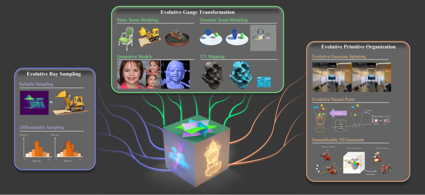
Figure 1. We present Evolutive Rendering Models (ERM), a framework with broad applications that enhances existing models by incorporating evolutive rendering elements, and unlocks new possibilities for previously unattainable tasks. ERM exhibits superior performance across diverse representation types (MLP-based, grid-based, and point-based models), as well as various rendering mechanism (volumetric rendering and splatting).

1. Introduction

The field of computer graphics has undergone a remarkable revolution with the advancement of differentiable rendering models highlighted by representative works (Mildenhall et al., 2020; Müller et al., 2022a; Kerbl et al., 2023). Such models are essential for accurate environment digitization and immersive XR experiences, and are increasingly relevant across a diverse array of industries including construction, entertainment, and robotics. It bridges the gap between real-world data acquisition and digital visual representation. The versatility and applicability of differentiable rendering in these domains underscore its significance as a transformative tool in modern graphics and machine learning applications.

Despite these advancements, a fundamental challenge persists in the development of rendering models: the reliance on one-fits-all, heuristic, hand-defined rules. These heuristics, while beneficial in offering a starting point for model design, often compromise the expressiveness and adaptability of the models. They tend to impose rigid constraints, limiting the capacity of these models to adapt and evolve in response to diverse and dynamically changing optimization state and rendering objectives.

In this work, we introduce Evolutive Rendering Models. The ERM is designed to evolve autonomously towards more optimal states, offering an alternative to traditional heuristic and rule-based methods. This work focuses on three prevalent elements in scene representation and rendering: (1) a gauge transformation (Zhan et al., 2023), denoting the conversion between distinct measuring systems, to perform space mapping to index radiance fields, (2) a sampling mechanism to perform ray sampling for volume rendering, and (3) a primitive organization in the space to perform point-based rendering. Central to this approach is the employment of differentiable version of above elements, which paves the way for a fully learnable system, adaptively guided by gradient-based optimization. Anchoring this innovative framework is a principled optimization paradigm termed as relay learning mechanism, meticulously devised through rigorous gradient analysis. This relay learning mechanism ensures robust and stable evolution of the rendering models across diverse test scenarios, marking a significant stride in the field.

Aligned with the three rendering elements, we include several concrete samples to demonstrate its potential applications: (1) Evolutive Gauge Transformation: we develop a parametric mapping technique between Euclidean 3D space and low-dimensional 2D space (Chan et al., 2022; Fridovich-Keil et al., 2023; Zhan et al., 2023). This technique employs learnable components for dynamic adaptation of the mapping process, facilitating flexible and expressive scene representation. (2) Evolutive Ray Sampling: we propose a gradient-guided sampling strategy to improve the efficiency of ray-marching techniques. This strategy notably enhances reconstruction quality in NeRF-based volumetric rendering (Müller et al., 2022a; Sun et al., 2022), promoting the rendering efficiency and overall quality in current methodologies. (3) Evolutive Primitive Organization: in the realm of point-based rendering, our approach innovates by incorporating a learnable component to optimize the densification and pruning phases (Xu et al., 2022; Kerbl et al., 2023). This adaptation is responsive to the current optimization state, thus improving both precision and efficiency. The practical applications of this approach range from promoting performance of existing models by incorporating evolutive rendering elements, to unlocking new possibilities for tasks that were unattainable with existing models. Our experiments are performed over a variety of representation types (MLP-based, grid-based, and point-based models), as well as different rendering types (volumetric rendering and splatting), highlighting the adaptability and broad applicability of our evolutive rendering approach.

In summary, our key contributions are:

• Introduction of the Evolutive Rendering Model (ERM) for autonomous evolution towards optimal rendering states;

• Integration of differentiable components as an alternative to heuristic and rule-based elements, facilitating a fully learnable system;

• Establishing a relay learning mechanism, rigorously grounded in gradient analysis, to facilitate robust and stable evolution in a myriad of rendering applications.

• Demonstration of the superiority of ERM through concrete examples within contemporary computer graphics, which span over a variety of representation types and rendering techniques.

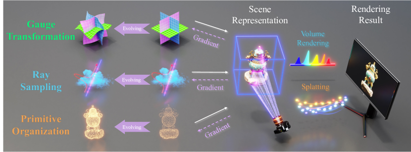
Figure 2. Evolutive Rendering Models covers three principal rendering elements: gauge transformation, ray sampling and primitive organization. All three elements can be applied in volume rendering, while splatting only employs evolutive gauge transformation and primitive organization.

2. Related Work

Recent work has significantly advanced the field of scene representation, particularly through the development of NeRF & 3DGS (Mildenhall et al., 2020; Kerbl et al., 2023) and their various extensions. These advancements have found widespread application in numerous areas of vision and graphics, notably in view synthesis (Yu et al., 2021a; Lindell et al., 2021; Fridovich-Keil et al., 2022; Reiser et al., 2021; Sun et al., 2022), generative models (Schwarz et al., 2020; Niemeyer and Geiger, 2021; Chan et al., 2021), and surface reconstruction (Wang et al., 2021; Oechsle et al., 2021; Yariv et al., 2021).

In contrast to the aforementioned application works, our proposed evolutive rendering models cater to the fundamental elements in scene representation and rendering, including gauge transformation, ray sampling, and primitive organization.

2.1. Gauge Transformation

Under the context of neural rendering, gauge transformation denotes the mapping between two coordinate systems. This concept is correlated with the prevailing paradigm of learning deformation for dynamic modeling (Tretschk et al., 2021; Tewari et al., 2022; Park et al., 2021; Pumarola et al., 2020; Peng et al., 2021), which actually learns a mapping within one coordinate system. A diverse array of gauge transformations has been extensively investigated in neural fields, serving various objectives like efficient rendering (Chan et al., 2022; Chen et al., 2022; Müller et al., 2022a; Zhan et al., 2023). A pre-defined mapping function is usually employed as the gauge transformation. A typical example is orthogonal mapping, which involves projecting a 3D space onto 2D planes as in (Chan et al., 2022; Peng et al., 2020). Expanding this concept, TensoRF (Chen et al., 2022) propels this research forward for fast and efficient optimization by projecting the 3D scene space into 2D planes and 1D vectors; Cao and Johnson (2023); Fridovich-Keil et al. (2023) propose to project 4D space onto 2D planes for dynamic modeling.

Concurrently, some studies also ventured into learning the gauge transformation for specialized tasks within neural fields. NeuTex (Xiang et al., 2021) and NeP (Ma et al., 2022), for instance, focus on learning the mapping from 3D points to 2D texture spaces. Neural Gauge Fields (Zhan et al., 2023) generally explores the problem of gauge transformation and its optimization. However, all above works necessitate certain regularizations to facilitate stable optimization, which is a cumbersome process and hinders it for practical applications. In this work, we introduce a relay learning mechanism which allows efficient optimization of gauge transformations without any regularizations, unlocking its potential for various gra-phic applications.

2.2. Ray Sampling

Ray sampling is pivotal in promoting the efficiency of volume rendering. The original NeRF (Mildenhall et al., 2020) employs a coarse-to-fine sampling strategy, selecting points based on their contribution to the final rendering.

However, the coarse sampling phase entails a cumbersome process of querying radiance fields per point along a ray. To address this, a series of work focuses on directly generating target samples for a given ray. NeuSample (Fang et al., 2021) suggests that the coarse stage can be substituted with a lightweight module parameterized by an MLP. Similarly, DONeRF (Neff et al., 2021) and TermiNeRF (Piala and Clark, 2021) propose replacing vanilla NeRF’s coarse sampling with a sampling network that predicts object surface depths. Yet, these methods hinge on the availability of depth maps, constraining their practical utility. In scenarios without depth priors, AdaNeRF (Kurz et al., 2022) introduces a sampler network that converts rays into discrete probabilities, albeit involving a complex optimization procedure. ProNeRF (Bello et al., 2023) opts for estimating sampled points in a coarse-to-fine manner, supplemented by multiview projection to capture geometric information. Overall, above approach, by sidestepping the structure of radiance fields, is prone to issues like geometry collapse and overfitting.

Conversely, another research trajectory maintains the coarse-to-fine sampling paradigm. NeRF in Detail (Arandjelović and Zisserman, 2021) conducts initial coarse sampling of a ray, followed by a network that refines target points from the coarsely sampled points’ features. MipNeRF 360 (Barron et al., 2022) suggests distilling information from the density field into a sampling field for ray sampling. However, the distillation loss employed is based on heuristics, presupposing an alignment between the sampling and density fields. Rather than relying on heuristic designs, RVS (Morozov et al., 2023) enables the gradient from the training objective to optimize the sampling field. Nevertheless, this method is primarily applicable to MLP-based radiance fields. In our work, we demonstrate the utility of training objective gradients for general representation types of sampling fields, employing a straightforward yet efficient strategy known as relay learning mechanism for optimization.

2.3. Point-based rendering

While neural radiance fields (NeRF) (Mildenhall et al., 2020) are prevalent, as highlighted in prior work, point-based primitives offer an efficient alternative, leveraging GPU hardware rasterization (Pineda, 1988). Traditional single-pixel point rendering faces challenges like holes in sparse point clouds (Catmull, 1974; Schaufler, 1998), addressed in part by convolutional neural networks (Aliev et al., 2020). However, these methods struggle with view consistency and generalization. The rise of NeRF has led to techniques like Point-NeRF (Xu et al., 2022), combining points with volumetric rendering, albeit at a loss of rasterization efficiency. Notably, EWA splatting (Zwicker et al., 2002) interprets point rendering through a signal reconstruction lens, employing Gaussian reconstruction kernels to reconstruct continuous signals from discrete samples. Recent advancements have focused on integrating differentiability into point-based rasterizers (Yifan et al., 2019; Wiles et al., 2020; Lassner and Zollhofer, 2021; Müller et al., 2022b; Kerbl et al., 2023). Notably, Kerbl et al. have developed an efficient differentiable point rasterizer, synergizing EWA Splatting with volume rendering. This innovation facilitates both rapid scene reconstruction and photorealistic novel-view synthesis in real-time.

Optimizing point-based inverse rendering models crucially depends on the organization of primitives. A common strategy involves periodic resampling through splitting and pruning, essential for optimization stability (Zheng et al., 2023; Kerbl et al., 2023). However, current splitting and pruning strategies are heuristic and not optimized concurrently. PixelsSplat (Charatan et al., 2023) critiques these strategies, proposing a differentiable parameterization of Gaussian primitives less prone to local minima. In our work, we introduce an innovative primitive organization procedure, integrating differentiable splitting and pruning within an evolutionary optimization framework.

3. Methodology

This section describes the methodology underlying the proposed Evolutive Rendering Model (ERM). As illustrated in Fig. 2, our framework covers three principal rendering elements including the gauge transformation, the ray sampling, and the primitive organization. The gauge transformation can be performed to transform discrete points to another coordinate system to index scene representation as shown in Fig. 3. Notably, ray sampling (in volume rendering) and primitive organization (in splatting) share essentially the same key operation in rendering pipelines, i.e., yielding desired discrete positions in the continuous space to perform rendering. The unified formulation of volume rendering and point-based (or splat-based) rendering can be written as:

(1) $$C=\sum_{i\in\mathcal{N}}c_{i}\alpha_{i}\prod_{j=1}^{i-1}(1-\alpha_{j}),$$

where $C$ is the color of a image pixel, $c_{i}$ is the color of discrete point in the space. In volume rendering, $\alpha_{i}$ can be computed according to the point density $\sigma$ as $\alpha_{i}=(1-exp(-\sigma_{i}\delta_{i}))$; in point-based rendering, $\alpha_{i}$ is given by evaluating a 2D Gaussian according to its covariance and per-point opacity.

As two different lines of research, ray sampling and primitive organization are incompatible in rendering models for most cases . For instance, volume rendering models can only employ gauge transformation and ray sampling, while the point-based rendering models can only employ gauge transformation and primitive organization.

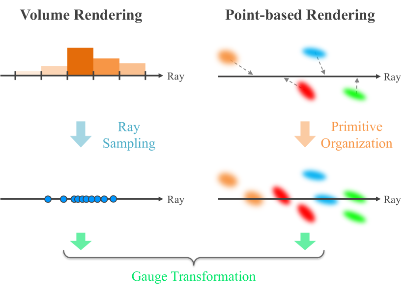
Figure 3. A conceptual illustration of rendering elements, including ray sampling in volume rendering, primitive organization in point-based rendering, and gauge transformations. Volumetric and point-based rendering can be performed in a unified manner: accumulating or blending discrete points relevant to the given ray.

3.1. Evolutive Gauge Transformation

Generally, a gauge defines a measuring system, e.g., pressure gauge and temperature gauge. In the context of neural rendering, a measuring system (i.e., gauge) is a specification of parameters to index a radiance field, e.g., 3D Cartesian coordinate in original NeRF (Mildenhall et al., 2020), triplane in EG3D (Chan et al., 2022), plane & vector in TensoRF (Chen et al., 2022). The transformation between different measuring systems is referred as Gauge Transformation. In radiance fields, gauge transformations are defined as the transformation from the original space to another gauge system to index radiance fields. This additional transform could introduce certain bonus to the rendering, e.g., low memory cost, high rendering quality, or explicit texture, depending on the purpose of the model.

Typically, the gauge transformation is performed via a pre-defined function, e.g., an orthogonal mapping in 3D. This pre-defined function is a general design for various scenes, which means it is not necessarily the best choice for a specific target scene. Moreover, it is a non-trivial task to manually design an optimal gauge transformation which aligns best with the complex training objective. We thus introduce the concept of Evolutive Gauge Transformation (EGT) to optimize a desired transformation directly guided by the final training objective.

The gauge transformation can be parameterized by an MLP-network & feature grid, or per-point property for the case of point-based rendering. For a point $x\in\mathbb{R}^{3}$ in the original space, the evolutive gauge transformation outputs the corresponding coordinate in the target space. The output coordinate can be the absolute value or a residual offset. On the other hand, the efficient optimization of EGT is a challenging task, previous works (Zhan et al., 2023) regularize the optimization process for implicit fields, which however is too heavy for practical applications. We thus introduce optimization strategies without clearly slowing down the training speed.

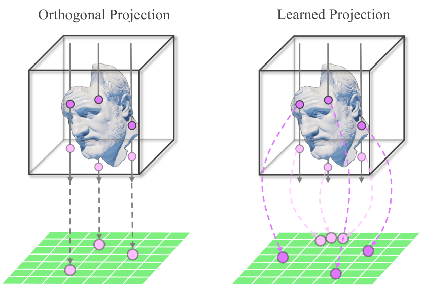
Figure 4. Motivation of evolutive gauge transformation. In this example, instead of mapping the 3D euclidean space to the 2D plane by orthogonal projection (left), we learn a more flexible and adaptive mapping (right).

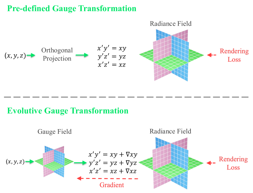
Figure 5. The illustration of predefined (upper) and evolutive (lower) gauge transformation. We implement the evolutive transformation by predicting an offset to the pre-defined transformation.

Generally, the gradient is unstable at the initial training stage, which is especially the case for grid-based representation as analyzed in Sec. 4. We thus introduce a deferred learning strategy for stable optimization of gauge transformation. As shown in Fig. 5, we train the model with a pre-defined gauge transformation (e.g. , orthogonal projection) at the initial stage. The gradient will become more stable when a coarse scene representation is learned. Thus, for the later stage, we replace the predefined gauge transformation with the learnable counterpart, and jointly optimize it with the scene representation. The training strategy can help to stabilize the training and accelerate the convergence for general representations, especially for grid-based representation.

3.2. Evolutive Ray Sampling

In volume rendering process, densely evaluating the radiance field network at query points along each camera ray is inefficient, as only few regions contribute to the rendered image. Thus, a coarse-to-fine sampling strategy (Mildenhall et al., 2020) is usually employed to increase rendering efficiency by allocating samples proportionally to their expected effect on the final rendering. To achieve coarse-to-fine sampling, a sampling field is included in the rendering pipeline. At first, a set of points are uniformly sampled along a ray $[t_{1},\cdots,t_{N}]$, to evaluate the sampling field. For piecewise constant approximation, point density within each bin $t_{i}\leq\hat{t}_{i}\leq t_{i+1}$ are approximated with constant density of $\sigma_{i})$. The evaluation of $[t_{1},\cdots,t_{N}]$ yields a discrete distribution of density along the ray, which gives the color weights $w_{i}$ of different point as:

(2) $$w_{i}=\alpha_{i}\prod_{j=1}^{i-1}(1-\alpha_{j})\quad\alpha_{i}=(1-exp(-\sigma_{i}\delta_{i}))$$

The color weights are normalized as $w_{i}=\nicefrac{{w_{i}}}{{\sum_{j=1}^{N_{c}}w_{j}}}$ to produce a piecewise-constant probability density function (PDF) along the ray. According to the PDF and corresponding CDF, a second set of locations are sampled from this distribution using inverse transform sampling, which allocates more samples to more visible regions.

To optimize the sampling fields, previous work either treat it as a radiance field trained with photometric loss or distilling the density knowledge from the radiance fields as shown in Fig. 7. Thus, all of them are making a heuristic assumption: the best of sampling fields should be aligned with the density fields. However, the objective of sampling field is to select the best set of points for the evaluation of radiance field, while the density field aims to yield the best rendering results. Thus, previous heuristic assumption will bias the optimization objective of sampling fields. On the other hand, it is non-trivial to manually design the training objective for the sampling fields, which should be determined by the radiance fields as sampling fields serve for radiance fields. To this end, we propose to backpropagate gradients from the radiance fields (i.e. , rendering loss) to optimize the sampling field directly, eliminating the need to heuristically design auxiliary loss supervision. However, for this case of piecewise constant approximation, the CDF is a discontinuous step function, which hinders the gradient backpropagation in the sampling process.

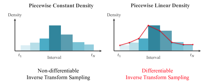
Figure 6. Differentiable sampling with piecewise linear approximation.

To achieve differentiable sampling, we adopt a piecewise linear density to approximate the opacity (Morozov et al., 2023; Uy et al., 2023), as illustrated in Fig. 6. Specifically, we compute $\sigma(t),t\in[t_{i},t_{i+1}]$ by interpolating the values between the interval points $t_{i}$ and $t_{i+1}$:

(3) $$\sigma(t^{\prime}_{i})=\sigma_{i+1}\frac{t_{i+1}-t}{t_{i+1}-t_{i}}+\sigma_{i}\frac{t-t_{i}}{t_{i+1}-t_{i}}.$$

Given these piecewise linear approximations of $\sigma_{i},i\in[1,N]$, we can yield a continuous PDF and CDF according to Eq. (2). With the continuous CDF, the sampling process with inverse transform is differentiable function with respect to the density field $\sigma_{i}$ and can back-propagate the gradients to optimize the sampling fields.

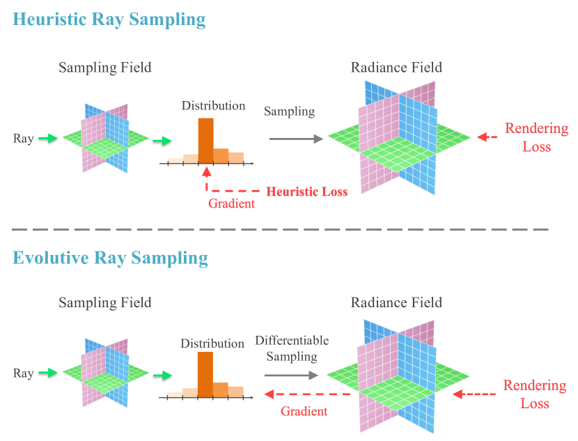
Figure 7. The illustration of pre-defined ray sampling and evolutive ray sampling.

This differentiable sampling algorithm can be smoothly integrated into the hierarchical sampling scheme originally proposed in NeRF. Here we do not change the final color approximation, utilizing the original one, but modify the way the coarse density network is trained. The method we introduce consists of two changes to the original scheme. Firstly, we replace sampling from piecewise-constant PDF along the ray defined by weights $w_{i}$ with differentiable sampling algorithm that uses piecewise linear approximation of $\sigma_{\bm{r}}$ and generates samples from $p_{r}(t)$ using inverse CDF. Secondly, we remove the auxiliary reconstruction loss imposed on the coarse network. Instead, we propagate gradients through sampling. This way, we eliminate the need for auxiliary coarse network losses and train the network to solve the actual task of our interest: picking the best points for evaluation of the fine network. All components of the model are trained together end-to-end from scratch.

3.3. Evolutive Primitive Organization

Point-based representations employ a set of geometric primitives (e.g. neural points in Point-NeRF (Xu et al., 2022), Gaussians splats in 3D-GS (Kerbl et al., 2023)) for scene rendering. These primitives compose of attributes that encode the geometry and radiance field, which can be rendered and optimized via volume render or rasterization operation. They are usually initialized from SFM and optimizing their attributes directly via gradient descent suffers from local minima. Previous techniques try to alleviate this issue in per-scene fitting by employing pre-defined optimization heuristics, such as point growing and pruning in Point-NeRF and Adaptive Density Control in 3D-GS. However, these heuristic operations can be sub-optimal because they are non-differentiable and may misalign with final training objective. Furthermore, their non-differentiable nature also impedes their applicability in cross-scene generalizable settings. We thus propose primitive organization evolution, where scene primitives will be implicitly grown and split during training while maintaining gradient flow directly from training objective. Our proposed approach not only overcomes the challenges posed by non-differentiability but also facilitates the extension of current techniques to feed-forward generalizable settings, which we will elaborate in Section 6. An illustration of evolutive primitive organization is shown in Fig. 8.

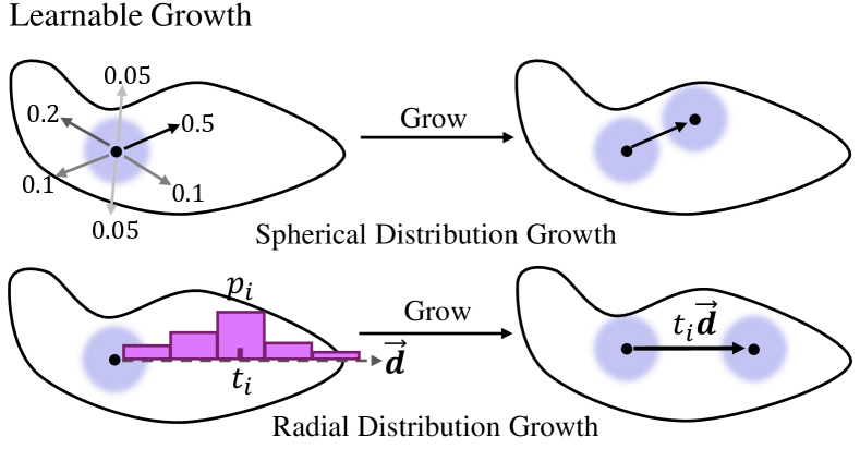
(a)

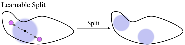
(b)

Figure 8. An illustration of evolutive primitive organization. In fig. (a), we elucidate evolutive primitive growth where we consider two fundamental forms of primitive growth distribution: spherical distribution growth has a pre-difined growth length and learn growth direction probability; radial distribution growth assums known growth direction and learn growth length probability. In fig. (b), we show evolutive primitive split, where a split shift term is learned to decide the location of newly-split primitives.

We denote the position of existing scene primitives as $\mu_{k}\in\mathbb{R}^{3}$. When primitive organization evolve to grow new primitives (eg. new primitives growth in under-reconstructed region), we learn a grown term $\delta\mu_{k}=td\in\mathbb{R}^{3}$ for the emergent primitives, where $d\in\mathbb{R}^{3}$ is the direction of grown term and $t\in\mathbb{R}$ is its length. The location $\mu^{\prime}_{k}$ of new primitives will be $\mu_{k}+\delta\mu_{k}$. The newly-grown primitives will be rendered during each iteration, which allows the grown term to be optimized by the final training objective throughout whole optimization process. Unfortunately, we find directly regressing grown term makes the training unstable, which is susceptible to local minima. Instead, we consider two most fundamental forms of primitive growing distribution: spherical distribution and radial distribution, elucidated in Fig. 8(a). In the context of spherical distribution growth, nascent primitives expand along a sphere enveloping the original primitives, with the growth length $t$ predefined and growth direction $d$ being learned. Conversely, in radial distribution growth, the grow direction is predefined, while the extent of growth $t$ along this direction will be learned. The combination of these two primary grow distribution actually spans the entirety of the potential growth space.

To stabilize the learning process, we choose to learn these two forms of distribution in discrete space. In more details, when to learn the spherical distribution of primitive growth, we first pre-define a set of $N$ uniformly distributed potential growing directions $\left\{d_{1},d_{2},...,d_{N}\right\}$, and each emergent primitive will learn a probability distribution of grow directions $Q\in\mathbb{R}^{N}$, where its i-th element $q_{i}$ represent the probability of growing along direction $d_{i}$. The actually grow direction $d$ is chosen to be the direction with maximum probability:

(4) $$d=d_{i},i=argmax(Q)$$

As Argmax operations is non-differentiable, we apply reparameterization trick by replacing Argmax operation with Softmax in gradient back-propagation. The pseudo code of the forward & backward propagation of the grow primitives is given in Algorithm 1. Similarly, for its counterpart of radial distribution growth, given grow direction $d$, we learn the growth distance by predicting the probability that new primitive will exist at distance $t$ along the direction. We discretize the extention along the direction into $N$ bins with distance $\left\{t_{1},t_{2},...,t_{N}\right\}$. And we learn a discrete grow distance probability $Q\in\mathbb{R}^{N}$, where $q_{i}$ represent the probability of growing with distance $t_{i}$. The pseudo code is also included in Algorithm 1. Please note that although these two primary grow distribution forms can span the entire potential growth space, experimentally in most cases we only need to employ one of them depending on the applications.

Algorithm 1 Pseudo-code of forward & backward propagation in primitive growth spherical/radial distribution optimizatation

  Input:potential grow directions $D=\left\{d_{1},d_{2},...,d_{N}\right\}$/potential grow distance $T=\left\{t_{1},t_{2},...,t_{N}\right\}$grow direction/distance probability $Q=[p_{1},p_{2},...,p_{N}]$ Forward propagation: 1. index = Argmax($Q$) 2. index-hard = One-Hot(index) 3. grow direction $d$ = Matmul(index-hard, $D$)/grow distance $t$ = Matmul(index-hard, $T$)Backward propagation: 1. index-soft = Softmax($Q$) 2. grow direction $d$ = Matmul(index-soft, $D$)/grow distance $t$ = Matmul(index-soft, $T$)

In addition to learned primitive growth, there are circumstances that require splitting the primitives. For example, 3D-GS propose a splitting operation that splits large primitives in over-reconstructed region into two smaller ones by dividing their scale with a pre-defined scaling factor of 1.6, and initialize their location by using the original 3D Gaussian as a PDF for sampling. This whole sampling process is no-differentiable and the splitting operation won’t directly align with optimization objective. Thus we additionally learn a differentiable splitting strategy by predicting the new position of split primitive (illustrated in Fig. 8(b)). Similarly to learned growing operation, we learn a split mean shift $\delta\mu$ and the position of two newly split primitive will be $\mu+\delta\mu$ and $\mu-\delta\mu$ separably. The new primitive will participate in rendering process within each training iteration, allowing gradient flow to update the shift term.

4. Optimization

For clarity, we denote the gauge transformation, the ray sampling, and the primitive organization as $\mathcal{T}$, $\mathcal{S}$, and $\mathcal{O}$, respectively. The optimization of above rendering elements relies on the gradients derived from rendering models. There are two main paradigms for rendering, including (1) sampling discrete points in the space to perform volume rendering (via point accumulation), (2) organizing discrete primitives in the space to perform splat-based rendering (via $\alpha$-blending). Given $\mathbf{u_{i}}=[c_{i},\sigma_{i}]$ and the unified formulation of volume rendering and point-based rendering $C=\sum_{i\in\mathcal{N}}c_{i}\alpha_{i}\prod_{j=1}^{i-1}(1-\alpha_{j})$, the function of per-point color contribution in can be written as $G(\mathbf{u_{i}})=c_{i}\alpha_{i}\prod_{j=1}^{i-1}(1-\alpha_{j})$. Note that $G$ is a differentiable function without learnable parameters. In the next subsections, we will discuss the gradient characteristics for element optimization in volume rendering and point-based rendering, respectively.

4.1. Gradient in Volume Rendering

Typical volume rendering is associated with a continuous representation of the scene, necessitating point sampling mechanism $\mathcal{S}$ to yield discrete samples (with optional gauge transformation $\mathcal{T}$). For clarity, we denote the joint process of ray sampling and gauge transformation as $\mathcal{ST}(r;\bm{\Theta}_{st})$, where $\bm{\Theta}_{st}$ and $r$ are the ray sampling & gauge transformation parameters and a given ray. Then, the process to yield a discrete point $p_{i}$ along ray $r$ can be written as $p=\mathcal{ST}(r;\bm{\Theta}_{st})$. The discrete point $p$ is further used to query the scene representation to yield color & density $\mathbf{u}=[c,\sigma]=f(p;\bm{\Theta}_{f})$, where $f$ and $\bm{\Theta}_{f}$ are the representation function and parameters, e.g., MLP in implicit neural fields or feature grid in explicit neural fields. Thus, the color contribution from $p$ can be formulated as:

(5) $$G(\mathbf{u})=G(f(p;\bm{\Theta}_{f}))=G(f(\mathcal{ST}(r;\bm{\Theta}_{st});\bm{\Theta}_{f})).$$

The gradient of $\mathbf{J}$ of the color contribution with respect to $\bm{\Theta}_{st}$ can be derived as:

(6) $$\mathbf{J}=\frac{\partial G(\mathbf{u})}{\partial\mathbf{u}}\frac{\partial f(p;\bm{\Theta}_{f})}{\partial p}\frac{\partial\mathcal{ST}(r;\bm{\Theta}_{st})}{\partial\bm{\Theta}_{st}}.$$

As the gradient term $\frac{\partial G(\mathbf{u})}{\partial\mathbf{u}}$ is obviously stable, the optimization depends on the terms $f$ and $\mathcal{ST}$ which will be analyzed according to their parameterization types in ensuing paragraphs.

4.1.1. Explicit Fields

For this case, $f$ and $\mathcal{ST}$ are parameterized by an explicit representation, like a feature grid. Considering the term $\frac{\partial f(p;\bm{\Theta}_{f})}{\partial p}$, $f$ can be written as an interpolation function. The oscillating gradient $\frac{\partial f(p;\bm{\Theta}_{f})}{\partial p}$ during interpolation across grid corners will severely preclude the optimization process, leading to slow convergence and local minima.

4.1.2. Implicit Fields

Generally, implicit fields provide smooth and global gradients as all points are querying the full MLP. However, to encode high frequency information in an MLP, a positional encoding is usually applied to $z_{i}$ before feeding into MLP. Thus, $f$ will be a composition of $f(p)=f^{\prime}\circ\gamma(p)$, $\gamma_{k}(p)=\big{[}\cos(2^{k}\pi p),\sin(2^{k}\pi p)\big{]}$. As shown in Lin et al. (2021), the positional encoding will amplify the gradient exponentially, which leads to unstable training.

4.2. Gradient in Point-based Rendering

In contrast to volume rendering, point-based rendering works with discrete representations directly, which requires a primitive organization $\mathcal{O}$ (with optional gauge transformation $\mathcal{T}$). For clarity, we denote the joint process of primitive organization and gauge transformation as $\mathcal{OT}(p;\bm{\Theta}_{ot})$, where $\bm{\Theta}_{ot}$ and $p$ are the primitive organization & gauge transformation parameters and a certain point. With an initialized discrete point $p$, the process to yield a new discrete point $p^{\prime}$ can be written as $\mathcal{OT}(p;\bm{\Theta}_{ot})=p^{\prime}$. To this end, the color contribution from this point can be formulated as

(7) $$G(p^{\prime},r)=G(\mathcal{OT}(p;\bm{\Theta}_{ot});r),$$

where $G$ is the splat-based rendering function, $r$ is the target ray. Compared with the case of volume rendering in eq. (5), there is no representation function $f$ in point-based rendering, which simplifies the gradient analysis. Then the gradient $\mathbf{J}$ of the color contribution with respect to $\bm{\Theta}_{ot}$ can be derived as:

(8) $$\mathbf{J}=\frac{\partial G(p^{\prime},r)}{\partial\bm{\Theta}_{ot}}=\frac{\partial G(p^{\prime},r)}{\partial p^{\prime}}\frac{\partial\mathcal{OT}(p;\bm{\Theta}_{ot})}{\partial\bm{\Theta}_{ot}}.$$

Notably, the gradient $\frac{\partial G(p^{\prime},r)}{\partial\bm{\Theta}_{ot}}$ has been carefully handled in (Yifan et al., 2019; Kerbl et al., 2023) to achieve stable optimization. For the term $\frac{\partial\mathcal{OT}(p;\bm{\Theta}_{ot})}{\partial\bm{\Theta}_{ot}}$, its optimization (or gradient characteristic) depends on the parameterization types of $\mathcal{OT}$.

The cases of grid-based and MLP-based parameterization have been analyzed in Sec. 4.1.1. Notably, the parameterization of $\mathcal{OT}$ can actually be discarded for point-based rendering, which means the parameters of $\mathcal{OT}$ can be simply saved as additional properties of discrete points. For the case without parameterization, the gradient in eq. (8) is stable as $\frac{\partial\mathcal{OT}(p;\bm{\Theta}_{ot})}{\partial\bm{\Theta}_{ot}}$ is a constant with respect to $\bm{\Theta}_{ot}$.

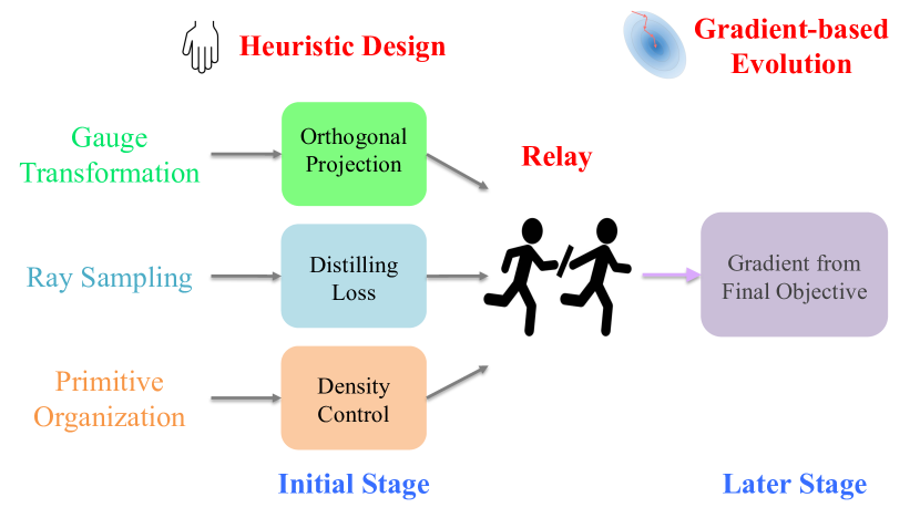
Figure 9. An illustration of relay learning mechanism. At the initial stage, the optimization is performed with heuristically designed elements, e.g., orthogonal projection for transformation, distilling loss for learning ray sampling, density control (Kerbl et al., 2023) for primitive organization. After certain iterations, the optimization is relayed to the gradient-based elements evolution.

4.3. Relay Learning Mechanism

Overall, we observe the consistent gradient problem (e.g. , fluctuation, large value), which are especially severe at the initial training stage, and will became smoother as the training goes. Motivated by our derivation and observation, we introduce a relay learning mechanism to facilitate the training process and avoid local minima when optimizing the rendering elements as shown in Fig. 9. Specifically, heuristically designed elements are employed at the initial training stage to achieve stable training and approximate the optimal solution, followed by the evolutive elements for accurate optimization towards the optimal solution. This mechanism ensures that the optimization will not suffer from the gradient problem at initial stage, and can effectively utilize the smooth gradient at later stages. By default, we perform the optimization relay around the first 10% steps.

5. Experimental Evaluation

We evaluate the effectiveness of ERM by replacing the heuristic design in existing rendering models with our evolutive elements.

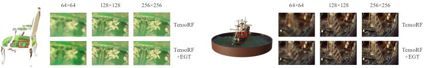
Figure 10. Comparison between renderings with the inclusion of EGT under different plane size.

5.1. Evolutive Gauge Transformation

To validate the effectiveness of our evolutive gauge transformation (EGT), we replace the orthogonal projection in TensoRF, KPlanes, and EG3D with our learnable mapping, to perform static scene modeling, dynamic modeling, and generative modeling, respectively.

Models	Setting	Time	PSNR$\uparrow$	SSIM$\uparrow$
Static Modeling on Synthetic NeRF
PlenOctrees	N/A	$\sim$15 hr	31.71	0.958
Plenoxels	N/A	11.4 min	31.71	0.958
DVGO	N/A	15.0 min	31.95	0.957
Mip-NeRF	N/A	2.89 hr	33.06	0.960
TensoRF	256 $\times$ 256	12.5 min	33.01	0.963
TensoRF+EGT	256 $\times$ 256	13.1 min	33.38	0.964
Dynamic Modeling on D-NeRF
KPlanes	256 $\times$ 256	36.2 min	31.03	0.946
KPlanes+EGT	256 $\times$ 256	36.6 min	31.31	0.947
Models	Setting	Time	FID$\downarrow$
Generative Modeling on FFHQ
EG3D	256 $\times$ 256	46 hr	7.051
EG3D+EGT	256 $\times$ 256	54 hr	6.546

Table 1. Evaluation of our evolutive gauge transformation at various tasks including static scene modeling, dynamic modeling, and generative modeling. TensoRF, KPlanes, and EG3D serve as the base model respectively. The setting indicates the size of feature planes. The plane size for modeling gauge transformation is kept the same as the base model by default.

	Sampling		Synthetic NeRF
Models	Coarse	Final	Time$\downarrow$	PSNR$\uparrow$	SSIM$\uparrow$
NeRF	32	64	8.81 hr	28.78	0.933
NeRF+ERS	32	64	8.43 hr	30.29	0.941
NeRF	64	64	10.5 hr	29.76	0.941
NeRF+ERS	64	64	10.1 hr	30.90	0.946
NeRF	96	64	12.0 hr	30.79	0.946
NeRF+ERS	96	64	11.6 hr	31.21	0.947

	Sampling		Synthetic NeRF			D-NeRF
Models	Coarse	Final	Time$\downarrow$	PSNR$\uparrow$	SSIM$\uparrow$	Time$\downarrow$	PSNR$\uparrow$	SSIM$\uparrow$
KPlanes	32	48	27 min	27.93	0.950	41 min	29.13	0.962
KPlanes+ERS	32	48	26 min	30.70	0.957	39 min	30.21	0.964
KPlanes	64	48	28 min	30.02	0.958	39 min	30.49	0.967
KPlanes+ERS	64	48	28 min	31.85	0.961	41 min	30.95	0.969
KPlanes	96	48	30 min	31.84	0.961	42 min	31.03	0.969
KPlanes+ERS	96	48	30 min	32.29	0.962	42 min	31.29	0.970

Table 2. The rendering performance by integrating evolutive ray sampling. ‘Coarse’ and ‘Final’ denote the number of points for sampling fields and radiance fields.

5.1.1. Static Scene Modeling

We first evaluate our evolutive gauge transformation on the static scenes from the Synthetic NeRF dataset (Mildenhall et al., 2020). Here, we use TensoRF (Chen et al., 2022) as the baseline model, with a plane size of $256\times 256$ and a plane dimension of 64. For the gauge transformation, we adopt the same model structure and plane size as the base model. The model is trained with a pre-defined orthogonal projection for the first 3000 steps, and subsequently the optimization transitions into using our proposed evolutive gauge transformation (EGT) to learn a flexible mapping. Intuitively, with the orthogonal mapping as the initizliation, we only learn a residual transformation term as illustrated in Fig. 5.

As shown in Table 1, the inclusion of EGT leads to a clear gain in the rendering quality of TensoRF, while only slightly reducing the training speed. Notably, the performance gain will be more distinct with decreasing feature plane sizes. We conjecture that the gradient oscillation around the grid corner will be mitigated with a small plane size, which leads to more stable optimization as analyzed in Sec. 4.1.1.

5.1.2. Dynamic Scene Modeling.

For dynamic scene modeling on the D-NeRF dataset (Pumarola et al., 2020), we set KPlanes as the base model with a plane size of $256\times 256$ and a feature dimension of 16 . The EGT employs the same model structure and plane size as the base model. As shown in Table 1, consistent performance improvements can be observed with the integration of EGT.

5.1.3. Generative Scene Modeling.

EG3D (Chan et al., 2022) serves as the base model for 3D generative modeling. Specifically, the Triplane structure and plane size ($256\times 256$) in EG3D is also adopted for the gauge transformation. The Triplane for gauge transformation is generated from the latent code with the generator in StyleGAN2. The training is performed with predefined orthogonal projection at the initial stage (10% of total iteration).

As shown in Table 1, the FID of the generated images can be improved by 0.505, while the training time will be increased by 8 hours as generating additional Triplanes with StyleGAN2 for the gauge transformation is a cumbersome process.

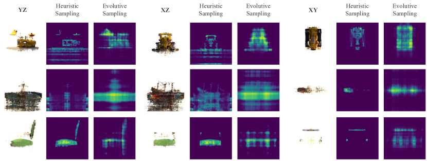
Figure 11. The illustration of learned sampling fields in heuristic design and our evolutive method. We visualize three 2D orthogonal cross sections (i.e. , YZ, XZ, and XY) of the sampling fields. The scenes include Lego, Ship, and Chair from the Synthetic NeRF dataset.

5.2. Evolutive Ray Sampling

We evaluate the performance of ERS on static scene modeling and dynamic scene modeling.

5.2.1. Static Scene Sampling

We perform experiments on the Synthetic NeRF dataset with NeRF and KPlanes as the base models. The plane size in KPlanes is set as $256$ with a feature dimension of 32. The sampling field adopts a plane size of $64\times 64$ with a feature dimension of 8. Specifically, both NeRF and KPlanes are equipped with sampling fields to perform coarse-to-fine sampling. To train the sampling fields, NeRF and KPlanes adopt a recontruction loss and distillation loss, respectively. NeRF+ERS and KPlanes+ERS remove these reconstruction losses and the distillation loss, as they can directly train the sampling fields by propagating gradient from the final training loss through the sampling process.

As shown in Table 2, the rendering quality and training time are improved consistently with the inclusion of ERS. We also ablate the effect of different number of coarse sampling ppoints, and observe that the ERS is more robust to the number of sampling points compared with the previous heuristic design. Notably, the NeRF training speed is also slightly improved as rendering operations in the reconstruction loss are reduced.

We also visualize and compare the learned sampling fields in Fig. 11. Specifically, we take three 2D orthogonal cross-sections (i.e. , YZ, XZ, and XY section) of the volume, which are uniformly sampled to query the sampling fields to get color and density. As shown in Fig. 11, the learned sampling fields with heuristic design are not well aligned with the scene geometry & surface as it is trained with reconstruction loss. As the comparison, the sampling fields learned with ERS tends to be smoothly distributed around scene surface. We conjecture this geometry slack of sampling fields is more beneficial for flexible volume rendering as there is no harsh geometry constraint.

5.2.2. Dynamic Scene Sampling

We validate the effectiveness of ERS with KPlanes as the base model on D-NeRF dataset. The KPlanes and sampling fields settings are similar to case of static scene modeling, just including an additional time dimension of size 50 for KPlanes and 25 for sampling fields. As shown in Table 2, the performance gain is also consistent with the inclusion of ERS.

	Mip-NeRF360						Tanks&Temples
Method	SSIM$\uparrow$	PSNR$\uparrow$	LPIPS$\downarrow$	Train	FPS	Mem	SSIM$\uparrow$	PSNR$\uparrow$	LPIPS$\downarrow$	Train	FPS	Mem
Plenoxels	0.626	23.08	0.463	25m49s	6.79	2.1GB	0.719	21.08	0.379	25m5s	13.0	2.3GB
INGP-Base	0.671	25.30	0.371	5m37s	11.7	13MB	0.723	21.72	0.330	5m26s	17.1	13MB
INGP-Big	0.699	25.59	0.331	7m30s	9.43	48MB	0.745	21.92	0.305	6m59s	14.4	48MB
M-NeRF360	0.792	27.69	0.237	48h	0.06	8.6MB	0.759	22.22	0.257	48h	0.14	8.6MB
3D-GS	0.815	27.21	0.214	41m33s	134	734MB	0.841	23.14	0.183	26m54s	154	411MB
3D-GS+EPO	0.838	27.45	0.208	47m24s	140	691MB	0.853	24.10	0.193	35m17s	161	380MB

	Synthetic NeRF
Method	SSIM$\uparrow$	PSNR$\uparrow$	LPIPS$\downarrow$
Plenoxels	0.958	31.71	0.049
Mip-NeRF	0.960	33.06	0.043
P-NeRF	0.967	30.71	0.081
P-NeRF+EPO	0.969	31.53	0.077
3D-GS	0.968	33.32	0.040
3D-GS+EPO	0.973	33.95	0.037

Table 3. EPO demonstrates superior performance on task of single scene radiance field modeling in both 3D Gaussian Splatting (3D-GS) framework and point-NeRF (P-NeRF) framework, we test on real-world mipnerf360 (Barron et al., 2022), Tanks&Temples (Knapitsch et al., 2017) scenes as well as synthetic scenes from Synthetic-NeRF (Mildenhall et al., 2020) dataset.

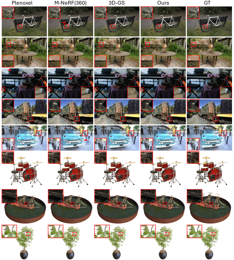
Figure 12. We show qualitative comparisons of our (Evolutive 3D Gaussian Splatting) to previous methods and the corresponding ground truth images from held-out test views. The scenes are, from the top down: Bicycle, Garden, Bonsai from the Mip-NeRF360 dataset; Train and Truck from Tanks&Temples; Drums, Ship, Ficus from NeRF Synthetic dataset. Differences in quality highlighted by arrows/insets.

5.3. Evolutive Primitive Organization

To evaluate the effectiveness of evolutive primitive organization (EPO), we test our component on both 3D Gaussian Splatting (3D-GS) framework and point-NeRF (P-NeRF) framework on the task of single scene radiance field rendering.

5.3.1. Evolutive 3D Gaussian Splatting

For 3D-GS, we regard each Gaussian as scene primitive and both the growing and splitting process will be learned during the whole optimization process. The original 3D-GS method will directly clone the Gaussians during the growing operation and does not have differentiable sampling and splitting operations. In our learned growing process, we will learn a position term $\delta\mu$ that defines the posituion of the newly split Gaussians. To do that, we apply spherical distribution growth to learn growth directions of new Gaussians. We implement the grown probability $Q$ as an attribute of existing Gaussians and directly optimize it throughout whole optimization process. When using Gaussians to learn radiance field, the newly-grown Gaussians should not be too far away from old Gaussians. Thus to learn a reasonable growth distance, instead of applying radial distribution growth, we can directly learn the distance by using standard deviation of original Gaussians as a constraint. More specifically, we set $\|\delta\mu\|=v*(1/1+exp(-s))$, where $s$ is learnable parameter in our implementation and $v$ is two times maximum standard deviation of original Gaussians. The other properties (scales, sh coefficients etc.) of newly-grown Gaussians are copied from original ones.

In addition to the learned growth, we also propose a learned splitting operation in our model. As mentioned in Sec. 3.3, we learn a split mean shift term that decide the position of newly-split Gaussians. The split mean shift is formulated as $\delta\mu_{k}=R(\sigma_{k}*(1/1+exp(-s^{\prime})))$, where $\sigma_{k}$ and $R$ are the standard deviation and rotation matrix of original Gaussians. $s^{\prime}$ is the learned parameter that control the length of the split shift. In addition to that, we also learn a scaling factor $\phi=1.2*(1/1+exp(-v))+1$ for each split Gaussian, where $v$ is the learned scalar parameter, and the newly split Gaussian scale will be divided by scaling factor $\phi$. Similar to that in 3D-GS, our differentiable growing and splitting operations focus on not well reconstructed region with large view-space positional gradients.

We follow the same training and evaluation setup as in 3D-GS. Similiar to that in 3D-GS, we initialize the position of 3D Gaussians using SFM points except for NeRF synthetic scenes where the Gaussian positions are randomly initialized. We set the number of potential directions $N$ to be 128 and do the growing and splitting operation every 100 training iterations. Each scene is optimized for 30k iterations.

Results We test our model on both real-world scenes from previously published datasets, including full set of scenes from Mip-NeRF360 dataset (Barron et al., 2022), eight scenes from LLFF dataset (Mildenhall et al., 2019), two scenes from Tanks&Temples dataset (Knapitsch et al., 2017), and synthetic scenes from the synthetic Blender dataset (Mildenhall et al., 2020). Those scenes have various capture styles, and cover both bounded indoor scenes and large unbounded outdoor environments.

Real-World Scenes We compare our method against several state-of-the-art techniques including Mip-NeRF360, 3D-GS as well as recent fast NeRF methods: InstantNGP and Plenoxels. We report results for a basic configuration of InstantNGP (Base) as well as a slightly larger network suggested by the authors (Big). We take every 8th images for test set and others for train set and compare with the standard PSNR, L-PIPS, and SSIM metrics, please see Table 3 and Table 4.

In contrast to Mip-NeRF 360, our model attains comparable results on the Mip-NeRF360 dataset and significantly outperforms it on the Tanks & Temples dataset. Furthermore, our model exhibits markedly faster training and inference speeds. Notably, compared to the original 3D-GS, our method achieves superior performance with, on average, fewer Gaussians per scene. This leads to reduced memory requirements and accelerated rendering speeds. This improvement is attributed to the efficacy of the evolution strategy, which enables more effective growth and splitting of Gaussians. We also show qualitative results of this comparison on test view in Fig. 12. Compared with previous methods, our model tends to preserve more visual detail from far away (Scene GARDEN, TRUCK and TRAIN) and recover some delicate thin structures (Scene BICYCLE, BONSAI), while original 3D-GS and Mip-NeRF360 may fail at those circumstances.

	LLFF
Method	PSNR$\uparrow$	SSIM$\uparrow$	LPIPS$\downarrow$
3D-GS	25.82	0.821	0.200
3D-GS+LGD	24.37	0.796	0.214
3D-GS+LSDG (Soft)	26.35	0.838	0.195
3D-GS+LSDG (Repara)	26.76	0.881	0.186
3D-GS+LSDG (Repara)+LSO	27.01	0.890	0.184

Table 4. Ablation study on different components of Evolutive 3D Gaussians Splatting on LLFF (Mildenhall et al., 2019) dataset.

Synthetic Blender Scenes In addition to realistic scenes, we also evaluate our approach on the synthetic NeRF dataset, results in Fig 3. Even though our approach starts training from 100K uniformly random Gaussians inside a volume that encloses the scene bounds, our approach can quickly converge to reasonable Gaussians, with better performance than all previous state-of-the-art methods. Similarly to the case in real-world scene, the Gaussians in our model grows and splits in a more efficient way, resulting in modeling the radiance field with fewer Gaussians which achieving better performance compared to 3D-GS.

Ablations In this part, we evaluate different components of our evolutive Gaussians design on LLFF dataset, including the learned spherical distribution growth (LSDG) and learned splitting operation (LSO), results shown in Table 4. For LSDG design, we compare against the straightforward method of directly learning growth direction (LGD). In our learned spherical distribution growth design, we choose to grow along the direction of maximum probability and propose the reparameterization (Repara-) strategy for optimization as shown in Alg.  1. To validate this proposal, we also test a soft variant to learn spherical distribution growth (Soft-), where grow direction is decided as weighted sum of all possible directions $d=\sum_{i=1}^{N}p_{i}d_{i}$.

When adopting the naive way of directly learning the growth direction, we find that the performance is even worse than baseline model. We speculate that it is because directly learning the growth direction has over-flexibility which makes the model to be vulnerable to local minimum. Compared to Soft version of learning spherical distribution growth, our reparameterization design adopts a more reasonable way of choosing growth direction, resulting in a better performance. The inclusion of learning splitting operation helps to further boost the performance. Our complete model is able to outperform original 3D-GS on PSNR by a significant margin of 1.2 dB, demonstrating the effectiveness of our evolutive primitive organization design.

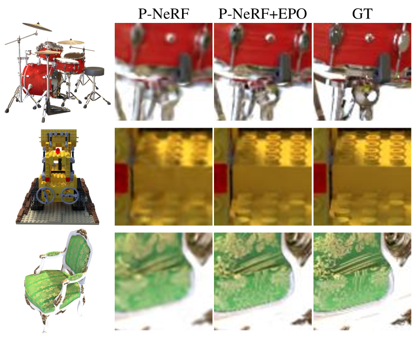
Figure 13. We show qualitative comparisons between P-NeRF (Xu et al., 2022) with our method that combines P-NeRF with evolutive primitive organization (EPO), as well as the corresponding ground truth images from held-out test views.

5.3.2. Evolutive Neural Point

In addition to evolutive 3D Gaussian Splatting, we also test Evolutive Primitive Organization in the framework of Point-NeRF (P-NeRF). In P-NeRF, the whole scene is composed of neural points feature that encode the radiance field. Instead of using splatting as in 3D-GS, P-NeRF adopts volume rendering mechanism where sampled points along the ray will query feature from neighbouring neural points, which will then be decoded into density and rgb color space. In P-NeRF, they adopts hand-designed growing and pruning operation to avoid holes and outliers in initial points. These operations have similar issue as in 3D-GS, that the operations are no-differentiable and may misalign with the final objective.

To alleviate this issue, we regard each neural point as scene primitive and learn the growing operation in per-scene optimization process. Particularly, the position of new neural points will be that of old neural points plus a learnable growth term $\delta\mu$. We apply spherical distribution growth to learn growth directions of new neural points. Similar to that in 3D-GS, the growth distance will be learned directly as $\|\delta\mu\|=v*(1/1+exp(-s))$, where $s$ is learnable parameter in our implementation and $v$ is two times initial voxel grid size in P-NeRF.

We follow the same per-scene optimization setup as in P-NeRF, where we adopt a loss function that combines the rendering and the sparsity loss. We do per-scene training for 20k iterations and perform point growing and pruning every 1K iterations. we evaluate our approach on the synthetic NeRF dataset, results in Table. 3. Compared to P-NeRF baseline method, the adoption of evolution neural points helps to improve performance on all metric, especially on PSNR and LPIPS by a good margin. This proves that our Evolutive Primitive Organization is effective in both volume rendering and splatting mechanism. Qualitative result is shown in Fig. 13.

	UV Mapping on DTU
Models	Regularization	PSNR$\uparrow$	SSIM$\uparrow$
NeuTex	✓	28.02	0.891
NGF	✓	27.74	0.887
Ours	$\times$	29.41	0.907

Table 5. Applications in UV mapping and editing.

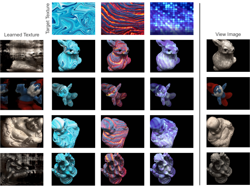
Figure 14. UV editing results.

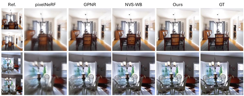
Figure 15. We show qualitative comparisons of ours to previous methods and the corresponding reference images from RealworldEstate10k dataset.

6. Applications

6.1. UV Mapping

Learning UV mapping is a non-trivial task in radiance fields. As UV mapping aims to connect the 2D space and 3D space, our evolutive gauge transformation is a good fit to achieve it. For this case, we aims to learn a mapping from 3D space to 2D plane, and adopt NeRF as the base model with a relay learning mechanism. Specifically, we train a NeRF with identical mapping (i.e. , without learning gauge transformation) for the first 30000 steps. As the geometry emerges which means the gradient becomes stable, we replace the identical mapping with the learnable transformation from 3D space to 2D plane in the color branch (Note the transformation is not applied in the density branch). After training, a UV map can be obtained by querying the radiance field with uniformly sampled points on the 2D plane.

We compare the performance of our method with NGF (Zhan et al., 2023) and Neutex (Xiang et al., 2021) as shown in Table 5. Our method outperforms previous methods on the rendering quality with UV mapping on DTU dataset (Aanæs et al., 2016). With the obtained UV maps, we easily edit the UV to the target texture as shown in Fig. 14.

6.2. Generalizable Gaussian Splatting

3D-GS has demonstrated remarkable performance and real-time rendering through rasterization-based rendering. However, the need for retraining on each new scene limits its practical applications. One way to tackle this bottleneck is to combine the 3D-GS representation with cross-scene generalizable NeRF models, which can directly synthesize novel views of unseen scenes. To achieve that, we need to build a model that can directly predict 3D Gaussian parameters in a feed-forward manner given images of new scene. Thus, the gradient should be able to be back-propagated to control the grow and prune of Gaussians. Our evolutive primitive organization exactly maintains the gradient from training objective where scene primitives will be implicitly grown. It turns to be a promising optimization solution for training generalizable 3D-GS model.

More specifically, given source view images and their camera parameter, our model first use an transformer-based encoder that aggregates multi-view image features via epipolar attention (Charatan et al., 2023) to predict pixel-wise feature. Then each feature will be passed through a decoder to directly predict the parameter of Gaussians along each ray. With known camera parameter, the direction along which to grow Gaussians has been decided. Thus we apply radial distribution growth method to predict the position of nascent Gaussians. We divide each ray into $N$ bins and learn the probability indicating the likelihood of Gaussians locating in each bin. And we decide the position of Gaussians by choosing the bin of maximum likelihood. The reparameterization strategy ( shown in Alg.  1) will be used here for optimization.

We evaluate our model on the task of wide-baseline novel view synthesis from stereo image pairs, conducting experiments on the RealEstate10k (Zhou et al., 2018) dataset. Following previous baseline (Du et al., 2023), we conduct experiments on image of resolution 256x256. In multi-view image encoder, we use a DINO  (Caron et al., 2021) pretrained ResNet-50 (He et al., 2016) followed by a ViT-B/8 vision transformer (Dosovitskiy et al., 2020). Adam optimizer (Kingma and Ba, 2014) is used for training.

We compare our model against three novel view-synthesis baselines, including GNPR (Suhail et al., 2022), pixelNeRF (Yu et al., 2021b) and NVS-WB (Du et al., 2023). GNPR uses a vision transformer-based backbone to compute epipolar features, and a light field-based renderer to compute pixel colors. pixelNeRF decodes pixel-aligned feature into neural radiance fields. NVS-WB uses a multi-view self-attention encoder and combines light field rendering with an epipolar transformer. As shown in Table. 6, our model is significantly more efficient than all the baselines models, inheriting the advantage of using Gaussians as scene representation. Particularly, our model is more than 100 times faster than the second best baseline model. Meanwhile, our model is able to outperform the baselines on all metrics. These are attributed to the differentiable nature of our evolutive primitive organization module. Qualitative results are shown in Fig. 15.

Method	PSNR$\uparrow$	SSIM$\uparrow$	LPIPS$\downarrow$	Inference Time (s) $\downarrow$
NVS-WB	24.78	0.820	0.213	1.32
GPNR	24.11	0.793	0.255	NA
pixelNeRF	20.43	0.589	0.550	5.30
Ours	25.64	0.853	0.148	0.11

Table 6. Application in generalizable gaussian splatting enabled by evolutive primitive organization: we show wide-baseline generalizable novel view synthesis from stereo images pairs on the real-world RealEstate10k (Zhou et al., 2018) dataset. Our model outperform all baseline methods in terms PSNR, LPIPS, and SSIM, while requiring much less inference time.

7. Limitations and Future Work

Although ERM has demonstrated broad applications ranging from enhancing performance of existing models to unlocking new possibilities for previously unattainable tasks, the current applications focus on the isolated utilization of individual evolutive elements among the three. Our current work reveals the substantial potential of evolutive rendering when applied to distinct components, however, we do not yet exploit its full potential. The integration of all of them remains a worthwhile avenue for future exploration and we will investigate this in the future. Moreover, by enabling the differentiability of previous manually crafted components, additional parameters will be learned within the whole framework. Consequently, the incorporation of an evolutive element typically results in longer training time.

8. Conclusion

In this work, we introduce evolutive rendering models (ERMs) that replace the heuristic designs in rendering models with learnable components that are fully aligned with the final rendering objective. In particular, we introduce a comprehensive learning framework that underpins the evolution of three principal rendering elements, including the gauge transformations, ray sampling mechanisms, and primitive organization. Our extensive experiments and thorough analysis show that the evolutive rendering models outperform their vanilla counterparts, hence demonstrating the large potential of evolutive rendering in computer graphics.

References

- (1)
- Aanæs et al. (2016) Henrik Aanæs, Rasmus RamsbØl Jensen, George Vogiatzis, Engin Tola, and Anders Bjorholm Dahl. 2016. Large-Scale Data for Multiple-View Stereopsis. Int. J. Comput. Vision 120, 2 (nov 2016), 153–168. https://doi.org/10.1007/s11263-016-0902-9
- Aliev et al. (2020) Kara-Ali Aliev, Artem Sevastopolsky, Maria Kolos, Dmitry Ulyanov, and Victor Lempitsky. 2020. Neural point-based graphics. In Computer Vision–ECCV 2020: 16th European Conference, Glasgow, UK, August 23–28, 2020, Proceedings, Part XXII 16. Springer, 696–712.
- Arandjelović and Zisserman (2021) Relja Arandjelović and Andrew Zisserman. 2021. Nerf in detail: Learning to sample for view synthesis. arXiv preprint arXiv:2106.05264 (2021).
- Barron et al. (2022) Jonathan T Barron, Ben Mildenhall, Dor Verbin, Pratul P Srinivasan, and Peter Hedman. 2022. Mip-nerf 360: Unbounded anti-aliased neural radiance fields. In Proceedings of the IEEE/CVF Conference on Computer Vision and Pattern Recognition. 5470–5479.
- Bello et al. (2023) Juan Luis Gonzalez Bello, Minh-Quan Viet Bui, and Munchurl Kim. 2023. ProNeRF: Learning Efficient Projection-Aware Ray Sampling for Fine-Grained Implicit Neural Radiance Fields. arXiv preprint arXiv:2312.08136 (2023).
- Cao and Johnson (2023) Ang Cao and Justin Johnson. 2023. Hexplane: A fast representation for dynamic scenes. In Proceedings of the IEEE/CVF Conference on Computer Vision and Pattern Recognition. 130–141.
- Caron et al. (2021) Mathilde Caron, Hugo Touvron, Ishan Misra, Hervé Jégou, Julien Mairal, Piotr Bojanowski, and Armand Joulin. 2021. Emerging properties in self-supervised vision transformers. In Proceedings of the IEEE/CVF international conference on computer vision. 9650–9660.
- Catmull (1974) Edwin Earl Catmull. 1974. A subdivision algorithm for computer display of curved surfaces. The University of Utah.
- Chan et al. (2022) Eric R Chan, Connor Z Lin, Matthew A Chan, Koki Nagano, Boxiao Pan, Shalini De Mello, Orazio Gallo, Leonidas J Guibas, Jonathan Tremblay, Sameh Khamis, et al. 2022. Efficient geometry-aware 3D generative adversarial networks. In Proceedings of the IEEE/CVF Conference on Computer Vision and Pattern Recognition. 16123–16133.
- Chan et al. (2021) Eric R Chan, Marco Monteiro, Petr Kellnhofer, Jiajun Wu, and Gordon Wetzstein. 2021. pi-gan: Periodic implicit generative adversarial networks for 3d-aware image synthesis. In Proceedings of the IEEE/CVF conference on computer vision and pattern recognition. 5799–5809.
- Charatan et al. (2023) David Charatan, Sizhe Li, Andrea Tagliasacchi, and Vincent Sitzmann. 2023. pixelSplat: 3D Gaussian Splats from Image Pairs for Scalable Generalizable 3D Reconstruction. arXiv preprint arXiv:2312.12337 (2023).
- Chen et al. (2022) Anpei Chen, Zexiang Xu, Andreas Geiger, Jingyi Yu, and Hao Su. 2022. Tensorf: Tensorial radiance fields. In Computer Vision–ECCV 2022: 17th European Conference, Tel Aviv, Israel, October 23–27, 2022, Proceedings, Part XXXII. Springer, 333–350.
- Dosovitskiy et al. (2020) Alexey Dosovitskiy, Lucas Beyer, Alexander Kolesnikov, Dirk Weissenborn, Xiaohua Zhai, Thomas Unterthiner, Mostafa Dehghani, Matthias Minderer, Georg Heigold, Sylvain Gelly, et al. 2020. An image is worth 16x16 words: Transformers for image recognition at scale. arXiv preprint arXiv:2010.11929 (2020).
- Du et al. (2023) Yilun Du, Cameron Smith, Ayush Tewari, and Vincent Sitzmann. 2023. Learning to render novel views from wide-baseline stereo pairs. In Proceedings of the IEEE/CVF Conference on Computer Vision and Pattern Recognition. 4970–4980.
- Fang et al. (2021) Jiemin Fang, Lingxi Xie, Xinggang Wang, Xiaopeng Zhang, Wenyu Liu, and Qi Tian. 2021. Neusample: Neural sample field for efficient view synthesis. arXiv preprint arXiv:2111.15552 (2021).
- Fridovich-Keil et al. (2023) Sara Fridovich-Keil, Giacomo Meanti, Frederik Rahbæk Warburg, Benjamin Recht, and Angjoo Kanazawa. 2023. K-planes: Explicit radiance fields in space, time, and appearance. In Proceedings of the IEEE/CVF Conference on Computer Vision and Pattern Recognition. 12479–12488.
- Fridovich-Keil et al. (2022) Sara Fridovich-Keil, Alex Yu, Matthew Tancik, Qinhong Chen, Benjamin Recht, and Angjoo Kanazawa. 2022. Plenoxels: Radiance fields without neural networks. In Proceedings of the IEEE/CVF Conference on Computer Vision and Pattern Recognition. 5501–5510.
- He et al. (2016) Kaiming He, Xiangyu Zhang, Shaoqing Ren, and Jian Sun. 2016. Deep residual learning for image recognition. In Proceedings of the IEEE conference on computer vision and pattern recognition. 770–778.
- Kerbl et al. (2023) Bernhard Kerbl, Georgios Kopanas, Thomas Leimkühler, and George Drettakis. 2023. 3D Gaussian Splatting for Real-Time Radiance Field Rendering. ACM Transactions on Graphics 42, 4 (2023).
- Kingma and Ba (2014) Diederik P Kingma and Jimmy Ba. 2014. Adam: A method for stochastic optimization. arXiv preprint arXiv:1412.6980 (2014).
- Knapitsch et al. (2017) Arno Knapitsch, Jaesik Park, Qian-Yi Zhou, and Vladlen Koltun. 2017. Tanks and temples: Benchmarking large-scale scene reconstruction. ACM Transactions on Graphics (ToG) 36, 4 (2017), 1–13.
- Kurz et al. (2022) Andreas Kurz, Thomas Neff, Zhaoyang Lv, Michael Zollhöfer, and Markus Steinberger. 2022. Adanerf: Adaptive sampling for real-time rendering of neural radiance fields. In European Conference on Computer Vision. Springer, 254–270.
- Lassner and Zollhofer (2021) Christoph Lassner and Michael Zollhofer. 2021. Pulsar: Efficient sphere-based neural rendering. In Proceedings of the IEEE/CVF Conference on Computer Vision and Pattern Recognition. 1440–1449.
- Lin et al. (2021) Chen-Hsuan Lin, Wei-Chiu Ma, Antonio Torralba, and Simon Lucey. 2021. Barf: Bundle-adjusting neural radiance fields. In Proceedings of the IEEE/CVF International Conference on Computer Vision. 5741–5751.
- Lindell et al. (2021) David B Lindell, Julien NP Martel, and Gordon Wetzstein. 2021. Autoint: Automatic integration for fast neural volume rendering. In Proceedings of the IEEE/CVF Conference on Computer Vision and Pattern Recognition. 14556–14565.
- Ma et al. (2022) Li Ma, Xiaoyu Li, Jing Liao, Xuan Wang, Qi Zhang, Jue Wang, and Pedro V Sander. 2022. Neural parameterization for dynamic human head editing. ACM Transactions on Graphics (TOG) 41, 6 (2022), 1–15.
- Mildenhall et al. (2020) B Mildenhall, PP Srinivasan, M Tancik, JT Barron, R Ramamoorthi, and R Ng. 2020. Nerf: Representing scenes as neural radiance fields for view synthesis. In European conference on computer vision.
- Mildenhall et al. (2019) Ben Mildenhall, Pratul P Srinivasan, Rodrigo Ortiz-Cayon, Nima Khademi Kalantari, Ravi Ramamoorthi, Ren Ng, and Abhishek Kar. 2019. Local light field fusion: Practical view synthesis with prescriptive sampling guidelines. ACM Transactions on Graphics (TOG) 38, 4 (2019), 1–14.
- Morozov et al. (2023) Nikita Morozov, Denis Rakitin, Oleg Desheulin, Dmitry Vetrov, and Kirill Struminsky. 2023. Differentiable Rendering with Reparameterized Volume Sampling. arXiv preprint arXiv:2302.10970 (2023).
- Müller et al. (2022b) Jan U Müller, Michael Weinmann, and Reinhard Klein. 2022b. Unbiased Gradient Estimation for Differentiable Surface Splatting via Poisson Sampling. In European Conference on Computer Vision. Springer, 281–299.
- Müller et al. (2022a) Thomas Müller, Alex Evans, Christoph Schied, and Alexander Keller. 2022a. Instant neural graphics primitives with a multiresolution hash encoding. ACM Transactions on Graphics (ToG) 41, 4 (2022), 1–15.
- Neff et al. (2021) Thomas Neff, Pascal Stadlbauer, Mathias Parger, Andreas Kurz, Joerg H Mueller, Chakravarty R Alla Chaitanya, Anton Kaplanyan, and Markus Steinberger. 2021. DONeRF: Towards Real-Time Rendering of Compact Neural Radiance Fields using Depth Oracle Networks. Computer Graphics Forum 40, 4 (2021), 45–59.
- Niemeyer and Geiger (2021) Michael Niemeyer and Andreas Geiger. 2021. Giraffe: Representing scenes as compositional generative neural feature fields. In Proceedings of the IEEE/CVF Conference on Computer Vision and Pattern Recognition. 11453–11464.
- Oechsle et al. (2021) Michael Oechsle, Songyou Peng, and Andreas Geiger. 2021. Unisurf: Unifying neural implicit surfaces and radiance fields for multi-view reconstruction. In Proceedings of the IEEE/CVF International Conference on Computer Vision. 5589–5599.
- Park et al. (2021) Keunhong Park, Utkarsh Sinha, Jonathan T Barron, Sofien Bouaziz, Dan B Goldman, Steven M Seitz, and Ricardo Martin-Brualla. 2021. Nerfies: Deformable neural radiance fields. In Proceedings of the IEEE/CVF International Conference on Computer Vision. 5865–5874.
- Peng et al. (2021) Sida Peng, Junting Dong, Qianqian Wang, Shangzhan Zhang, Qing Shuai, Xiaowei Zhou, and Hujun Bao. 2021. Animatable neural radiance fields for modeling dynamic human bodies. In Proceedings of the IEEE/CVF International Conference on Computer Vision. 14314–14323.
- Peng et al. (2020) Songyou Peng, Michael Niemeyer, Lars Mescheder, Marc Pollefeys, and Andreas Geiger. 2020. Convolutional occupancy networks. In European Conference on Computer Vision. Springer, 523–540.
- Piala and Clark (2021) Martin Piala and Ronald Clark. 2021. Terminerf: Ray termination prediction for efficient neural rendering. In 2021 International Conference on 3D Vision (3DV). IEEE, 1106–1114.
- Pineda (1988) Juan Pineda. 1988. A parallel algorithm for polygon rasterization. In Proceedings of the 15th annual conference on Computer graphics and interactive techniques. 17–20.
- Pumarola et al. (2020) Albert Pumarola, Enric Corona, Gerard Pons-Moll, and Francesc Moreno-Noguer. 2020. D-NeRF: Neural Radiance Fields for Dynamic Scenes. arXiv:2011.13961 [cs.CV]
- Reiser et al. (2021) Christian Reiser, Songyou Peng, Yiyi Liao, and Andreas Geiger. 2021. Kilonerf: Speeding up neural radiance fields with thousands of tiny mlps. In Proceedings of the IEEE/CVF International Conference on Computer Vision. 14335–14345.
- Schaufler (1998) Gernot Schaufler. 1998. Per-object image warping with layered impostors. In Rendering Techniques’ 98: Proceedings of the Eurographics Workshop in Vienna, Austria, June 29—July 1, 1998 9. Springer, 145–156.
- Schwarz et al. (2020) Katja Schwarz, Yiyi Liao, Michael Niemeyer, and Andreas Geiger. 2020. Graf: Generative radiance fields for 3d-aware image synthesis. Advances in Neural Information Processing Systems 33 (2020), 20154–20166.
- Suhail et al. (2022) Mohammed Suhail, Carlos Esteves, Leonid Sigal, and Ameesh Makadia. 2022. Generalizable patch-based neural rendering. In European Conference on Computer Vision. Springer, 156–174.
- Sun et al. (2022) Cheng Sun, Min Sun, and Hwann-Tzong Chen. 2022. Direct voxel grid optimization: Super-fast convergence for radiance fields reconstruction. In Proceedings of the IEEE/CVF Conference on Computer Vision and Pattern Recognition. 5459–5469.
- Tewari et al. (2022) Ayush Tewari, Xingang Pan, Ohad Fried, Maneesh Agrawala, Christian Theobalt, et al. 2022. Disentangled3D: Learning a 3D Generative Model with Disentangled Geometry and Appearance from Monocular Images. In Proceedings of the IEEE/CVF Conference on Computer Vision and Pattern Recognition. 1516–1525.
- Tretschk et al. (2021) Edgar Tretschk, Ayush Tewari, Vladislav Golyanik, Michael Zollhöfer, Christoph Lassner, and Christian Theobalt. 2021. Non-rigid neural radiance fields: Reconstruction and novel view synthesis of a dynamic scene from monocular video. In Proceedings of the IEEE/CVF International Conference on Computer Vision. 12959–12970.
- Uy et al. (2023) Mikaela Angelina Uy, Kiyohiro Nakayama, Guandao Yang, Rahul Krishna Thomas, Leonidas Guibas, and Ke Li. 2023. NeRF Revisited: Fixing Quadrature Instability in Volume Rendering. In Thirty-seventh Conference on Neural Information Processing Systems.
- Wang et al. (2021) Peng Wang, Lingjie Liu, Yuan Liu, Christian Theobalt, Taku Komura, and Wenping Wang. 2021. NeuS: Learning Neural Implicit Surfaces by Volume Rendering for Multi-view Reconstruction. Advances in Neural Information Processing Systems 34 (2021), 27171–27183.
- Wiles et al. (2020) Olivia Wiles, Georgia Gkioxari, Richard Szeliski, and Justin Johnson. 2020. Synsin: End-to-end view synthesis from a single image. In Proceedings of the IEEE/CVF Conference on Computer Vision and Pattern Recognition. 7467–7477.
- Xiang et al. (2021) Fanbo Xiang, Zexiang Xu, Milos Hasan, Yannick Hold-Geoffroy, Kalyan Sunkavalli, and Hao Su. 2021. Neutex: Neural texture mapping for volumetric neural rendering. In Proceedings of the IEEE/CVF Conference on Computer Vision and Pattern Recognition. 7119–7128.
- Xu et al. (2022) Qiangeng Xu, Zexiang Xu, Julien Philip, Sai Bi, Zhixin Shu, Kalyan Sunkavalli, and Ulrich Neumann. 2022. Point-nerf: Point-based neural radiance fields. In Proceedings of the IEEE/CVF Conference on Computer Vision and Pattern Recognition. 5438–5448.
- Yariv et al. (2021) Lior Yariv, Jiatao Gu, Yoni Kasten, and Yaron Lipman. 2021. Volume rendering of neural implicit surfaces. In Advances in Neural Information Processing Systems, Vol. 34. 4805–4815.
- Yifan et al. (2019) Wang Yifan, Felice Serena, Shihao Wu, Cengiz Öztireli, and Olga Sorkine-Hornung. 2019. Differentiable surface splatting for point-based geometry processing. ACM Transactions on Graphics (TOG) 38, 6 (2019), 1–14.
- Yu et al. (2021a) Alex Yu, Ruilong Li, Matthew Tancik, Hao Li, Ren Ng, and Angjoo Kanazawa. 2021a. Plenoctrees for real-time rendering of neural radiance fields. In Proceedings of the IEEE/CVF International Conference on Computer Vision. 5752–5761.
- Yu et al. (2021b) Alex Yu, Vickie Ye, Matthew Tancik, and Angjoo Kanazawa. 2021b. pixelnerf: Neural radiance fields from one or few images. In Proceedings of the IEEE/CVF Conference on Computer Vision and Pattern Recognition. 4578–4587.
- Zhan et al. (2023) Fangneng Zhan, Lingjie Liu, Adam Kortylewski, and Christian Theobalt. 2023. General Neural Gauge Fields. In International Conference on Learning Representations.
- Zheng et al. (2023) Yufeng Zheng, Wang Yifan, Gordon Wetzstein, Michael J Black, and Otmar Hilliges. 2023. Pointavatar: Deformable point-based head avatars from videos. In Proceedings of the IEEE/CVF Conference on Computer Vision and Pattern Recognition. 21057–21067.
- Zhou et al. (2018) Tinghui Zhou, Richard Tucker, John Flynn, Graham Fyffe, and Noah Snavely. 2018. Stereo magnification: Learning view synthesis using multiplane images. arXiv preprint arXiv:1805.09817 (2018).
- Zwicker et al. (2002) Matthias Zwicker, Hanspeter Pfister, Jeroen Van Baar, and Markus Gross. 2002. EWA splatting. IEEE Transactions on Visualization and Computer Graphics 8, 3 (2002), 223–238.