Clip Body and Tail Separately: High Probability Guarantees for DPSGD with Heavy Tails

Abstract

Differentially Private Stochastic Gradient Descent (DPSGD) is widely utilized to preserve training data privacy in deep learning, which first clips the gradients to a predefined norm and then injects calibrated noise into the training procedure. Existing DPSGD works typically assume the gradients follow sub-Gaussian distributions and design various clipping mechanisms to optimize training performance. However, recent studies have shown that the gradients in deep learning exhibit a heavy-tail phenomenon, that is, the tails of the gradient have infinite variance, which may lead to excessive clipping loss to the gradients with existing DPSGD mechanisms. To address this problem, we propose a novel approach, Discriminative Clipping (DC)-DPSGD, with two key designs. First, we introduce a subspace identification technique to distinguish between body and tail gradients. Second, we present a discriminative clipping mechanism that applies different clipping thresholds for body and tail gradients to reduce the clipping loss. Under the non-convex condition, DC-DPSGD reduces the empirical gradient norm from ${\mathbb{O}\left(\log^{\max(0,\theta-1)}(T/\delta)\log^{2\theta}(\sqrt{T})\right)}$ to ${\mathbb{O}\left(\log(\sqrt{T})\right)}$ with heavy-tailed index $\theta\geq 1/2$, iterations $T$, and arbitrary probability $\delta$. Extensive experiments on four real-world datasets demonstrate that our approach outperforms three baselines by up to 9.72% in terms of accuracy.

1 Introduction

DPSGD abadi2016deep , as a mainstream paradigm of privacy-preserving deep learning, has wide applications in areas such as privacy-preserving recommender systems liu2023privaterec ; yi2021efficient , face recognition ghalebikesabi2023differentially ; harder2022pre ; tang2024differentially , and medical diagnosis adnan2022federated ; ji2022privacy ; meng2021improving ; ziller2021medical . Essentially, in each iteration of model training, DPSGD clips per-sample gradient under the $L_{2}$-norm constraint to obtain the maximum divergence between gradient distributions that differ by only one training data point and adds random noise within rigorous privacy bounds to the gradient for unbiased gradient estimation.

Most of existing DPSGD works bu2024automatic ; yang2022normalized ; xia2023differentially ; fang2022improved ; zhang2023differentially ; sha2023pcdp ; zhu2023improving ; koloskova2023revisiting rely on the assumption that the gradient noise follows a sub-Gaussian distribution to devise effective clipping strategies. However, recent studies zhang2020adaptive ; gurbuzbalaban2021heavy ; simsekli2019tail ; zhu2018anisotropic ; simsekli2020fractional ; camuto2021asymmetric ; panigrahi2019non ; barsbey2021heavy have shown that SGD gradient noise in deep learning often exhibit heavy-tailed distributions instead of light-tailed distributions (e.g., sub-Gaussian). This occurs even when the dataset originates from a light-tailed distribution, the gradients still diverge to a heavy-tailed distribution with infinite variance gurbuzbalaban2021heavy , which may slow down the convergence rate and impair training performance li2022high ; li2023high ; madden2020high ; gorbunov2020stochastic ; davis2020high ; li2020high . To cope with heavy-tailed dilemma in SGD, wang2021convergence ; li2023high ; gorbunov2020stochastic suggest employing larger clipping thresholds to get rid of the oscillations caused by heavy-tailed gradients on the training trajectory. Nevertheless, the clipping operation in DPSGD is closely tied to the magnitude of DP noise added to the gradients. Setting the clipping threshold too large can lead to a high-dimensional noise catastrophe zhou2020bypassing , which negatively impacts model performance and potentially disrupts the convergence of DPSGD algorithms. Therefore, practitioners need to carefully strike a balance between injected noise and clipping loss, as illustrated in Figure 1. The left sub-figure shows the trade-off under the light-tailed assumption. As the clipping threshold increases (i.e., when the red dotted line moves to the right), the clipping loss decreases, but the maximum divergence between neighboring distributions increases, leading to more DP noise being added. In the right sub-figure, under the same clipping threshold, the slower decay rate of the heavy tail distribution (blue line) introduces extra clipping loss, while it simultaneously reduces the maximum divergence compared to the light-tailed distribution. Consequently, the required DP noise magnitude is lower. Therefore, we aim to investigate the following key question in this paper: how to design an effective clipping mechanism under the heavy-tailed assumption to balance the trade-off between clipping loss and DP noise magnitude in DPSGD?

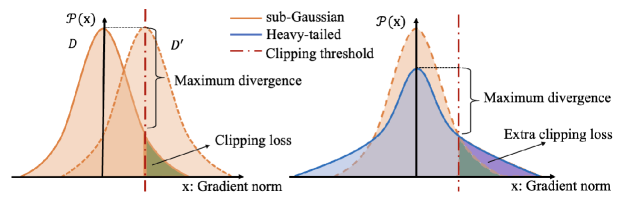
Figure 1: The trade-off between clipping loss and noise magnitude under heavy-tailed distributions.

Although a set of DPSGD clipping mechanisms bu2024automatic ; yang2022normalized ; xia2023differentially have been proposed under the light-tailed assumption, none of them can be adapted to our problem. Specifically, bu2024automatic ; yang2022normalized ; xia2023differentially focus on small-norm gradients (i.e., those near the center of the distribution) and normalize them to be around 1. These approaches reduce the maximum divergence, thereby requiring less noise to be injected. However, they do not account for heavy-tailed gradients and thus cannot optimize the clipping loss. Another line of work directly estimates the actual norm of the per-sample gradient and utilizes it as the clipping threshold to reduce the clipping loss. For instance, Andrew et al. andrew2021differentially estimate the true gradient trajectory by collecting the norms of historical gradients. However, this approach requires knowing the upper bound of historical norms for adding noise, which is highly uneconomical under heavy-tailed distributions, as the upper bound for moment generating function (MGF) vladimirova2020sub can be immeasurable, making the scale of DP noise unbearable.

In this paper, we propose a novel approach, named Discriminative Clipping (DC)-DPSGD, to effectively balance the trade-off between clipping loss and required DP noise under the heavy-tailed assumption. The key idea is to utilize different clipping thresholds for the body gradients and tail gradients respectively, retaining more information from tail gradients that can withstand more severe DP noise. We introduce two techniques in DC-DPSGD to achieve this goal. First, we design a subspace identification technique to identify potential heavy-tailed gradients with high probability guarantees. We note that the body of heavy-tailed distributions exhibits characteristics similar to those of light-tailed distributions, and the main difference lies in the decay rate at the tails. Therefore, we extract orthogonal random vectors from heavy-tailed distributions (e.g., sub-Weibull distribution) to construct a random projection subspace, and compute the trace of the second-moment matrix between gradients and this subspace to distinguish heavy-tailed gradients. Second, we present a discriminative clipping mechanism, which applies a large clipping threshold for the identified heavy-tailed gradients and a smaller one for the remaining light-tailed gradients. We theoretically analyze the choice of the two clipping thresholds and the convergence of DC-DPSGD with a tighter bound under the high probability theory. Our contributions can be summarized as follows.

• We propose DC-DPSGD with a subspace identification technique and a discriminative clipping mechanism to optimize DPSGD under the heavy-tailed assumption. To our knowledge, this is the first work to rigorously address heavy tails in DPSGD with a high probability theory guarantee.

• We theoretically analyze the convergence of DC-DPSGD and show that DC-DPSGD reduces the empirical gradient norm from $\mathbb{O}\left(\log^{\max(0,\theta-1)}(T/\delta)\log^{2\theta}(\sqrt{T})\right)$ to $\mathbb{O}\left(\log(\sqrt{T})\right)$ with heavy-tailed index $\theta\geq 1/2$, iterations $T$, and arbitrary probability $\delta$, under the non-convex condition.

• We conduct extensive experiments on four real-world datasets, where DC-DPSGD consistently outperforms four baselines with up to 9.72% accuracy improvements, demonstrating the effectiveness of our proposed approach.

2 Related Work

Heavy-tailed noise and high probability bounds. Recently, from the perspective of escaping from stationary points and Langevin dynamics, the noise in neural networks is more inclined to anisotropic and non-Gaussian properties gurbuzbalaban2021heavy ; simsekli2019tail ; zhu2018anisotropic ; panigrahi2019non ; gorbunov2020stochastic ; zhang2020adaptive , with specific heavy-tailed phenomena discovered and defined in gradient descent in deep neural networks. Current research has primarily focused on heavy-tailed convex optimization in privacy-preserving deep learning lowy2023private ; wang2020differentially ; kamath2022improved . Building upon wang2020differentially , Kamath et al. kamath2022improved relax the assumption of Lipschitz condition and sub-Exponential distribution to a more general $\alpha$-th moment bounded condition. However, no work has been done investigating the convergence characteristics of heavy-tailed DPSGD under non-convex settings. Meanwhile, high probability bounds are more frequently discussed in optimization properties such as convex and non-convex learning with SGD. Specifically, li2022high considers gradient noise from heavy-tailed sub-Weibull distribution to present high probability bounds at fast rates, revealing trade-offs between optimization and generalization performance under broader assumptions. With bounded $a$-th moments assumption, li2023high provides a high probability theoretical analysis for variants like clipped SGD with momentum and adaptive step sizes. Nevertheless, most work in DPSGD still utilizes expectation bounds, which is not suitable for heavy-tailed assumptions.

Projection subspace in DPSGD. DPSGD has gained wide concerns for its detrimental impact on model accuracy. A series of works leverage projection techniques to improve performance. For instance, zhou2020bypassing ; yu2021not ; liang2020think ; song2022sketching ; yu2021large confine DPSGD training dynamics to more compact and condensed subspaces through projection. While ensuring the fidelity of training data compression, they decouple the irrelevant relationship between ambient features and DP noise, and reduce the optimization error of DPSGD under stringent privacy constraints. However, existing works rely on the assumption that public datasets are available for designing the techniques  golatkar2022mixed ; zhou2020bypassing ; yu2021not ; gu2023choosing , which is a rather strong, especially in sensitive domains. In contrast, our work does not rely on any public dataset.

Gradient clipping. Gradient clipping has attracted significant attention in both practical implementations and theoretical analyses for DPSGD chen2020understanding ; zhang2019gradient ; zhang2022understanding ; pichapati2019adaclip ; andrew2021differentially ; xiao2023theory ; koloskova2023revisiting . Since the tuning parameters in the classical Abadi’s clipping function abadi2016deep are complex, adaptive gradient clipping schemes have been proposed bu2024automatic ; yang2022normalized . These schemes scale per-sample gradients based on their norms. In particular, gradients with small norms are amplified infinitely. Building upon this, Xia et al. xia2023differentially control the amplification of gradients with small norms in a finite manner. Additionally, research on clipping bias has gradually gained importance. Wei et al. wei2022dpis and Koloskova et al. koloskova2023revisiting argue for the connection between sampling noise and clipping bias and mitigate clipping bias through group sampling. Sha et al. sha2023pcdp study pre-projecting per-sample gradient before clipping to reduce clipping errors in DPSGD. Furthermore, fang2022improved has shown that naive gradient clipping can accelerate vanilla SGD convergence under heavy-tailed distributions. However, no work has specifically optimized gradient clipping under the heavy-tailed assumption of DPSGD. Due to the scale of noise required to achieve differential privacy, trivial clipping methods and analyses are not applicable.

3 Preliminaries

3.1 Notations

Let $D$ be a private dataset, which consists of $n$ training data $S=\{z_{1},...,z_{n}\}$ with a sample domain $Z$ drawn i.i.d. from the underlying distribution $\mathcal{P}$. Since $\mathcal{P}$ is unknown and inaccessible in practice, we minimize the following empirical risk in a differentially private manner:

$$L_{S}(\mathbf{w}):=\frac{1}{n}\sum^{n}_{i=1}\ell(\mathbf{w},z_{i}),$$ (1)

where the objective function $\ell(\cdot):(\mathbf{w}\subseteq W,Z)\rightarrow\mathbb{R}$ is possible non-convex and $W\subseteq\mathbb{R}^{d}$ represents the model parameter space. Then, we denote $\nabla\ell$ as the gradient of $\ell$ with respect to $\mathbf{w}$. In addition, we introduce some notations regarding the projection subspace. Let $V_{k}\in\mathbb{R}^{d\times k}$ denotes $k$-dimensional random projection sampled from heavy-tailed distributions. The empirical second moment of $V^{T}_{k}\nabla\ell$ is given by $V^{T}_{k}\nabla\ell\nabla\ell^{T}V_{k}$. The total variance in the empirical projection subspace is generally measured by the trace of the second moment denoted as $\text{tr}(V^{T}_{k}\nabla\ell\nabla\ell^{T}V_{k})$.

DPSGD lies in strict mathematical definitions dwork2006calibrating ; abadi2016deep and composition theorems kairouz2015composition ; mironov2017renyi ; dong2019gaussian . Definition 3.1 gives a formal definition of differential privacy (DP).

Definition 3.1 (Differential Privacy).

A randomized algorithm $M$ is $(\epsilon,\delta)$-differentially private if for any two neighboring datasets $D$, $D^{\prime}$ differ in exactly one data point and any event $Y$, we have

$$\mathbb{P}(M(D)\in Y)\leq\exp({\epsilon})\cdot\mathbb{P}(M(D^{\prime})\in Y)+\delta,$$ (2)

where $\epsilon$ is the privacy budget and $\delta$ is a small probability.

3.2 Assumptions

We focus on the sub-Weibull distribution in this work, which extends the sub-Gaussian and sub-Exponential families to potentially heavier-tailed distributions. Sub-Weibull distributions are characterized by a positive tail index $\theta$, with $\theta=\frac{1}{2}$ represents sub-Gaussian distributions, $\theta=1$ represents sub-Exponential distributions, and $\theta>1$ represents heavier-tailed distributions. Typically, sub-Gaussian distributions are light-tailed, whereas heavy-tailed distributions occur when $\theta>\frac{1}{2}$.

Assumption 3.1 (Sub-Weibull Gradient Noise).

Conditioned on the iterates, we make an assumption that the gradient noise $\nabla\ell(\mathbf{w}_{t})-\nabla L(\mathbf{w}_{t})$ satisfies $\mathbb{E}[\nabla\ell(\mathbf{w}_{t})-\nabla L(\mathbf{w}_{t})]=0$ and $\|\nabla\ell(\mathbf{w}_{t})-\nabla L(\mathbf{w}_{t})\|_{2}\sim\text{subWeibull}(\theta,K)$ for some positive K, such that $\theta>\frac{1}{2}$, and have

$$\mathbb{E}_{t}[\exp((\|\nabla\ell(\mathbf{w}_{t})-\nabla L(\mathbf{w}_{t})\|_{2}/K)^{\frac{1}{\theta}})]\leq 2.$$

Assumption 3.1 is a relaxed version of gradient noise following sub-Gaussian distributions, that is $\mathbb{E}_{t}[\exp((\|\nabla\ell(\mathbf{w}_{t})-\nabla L(\mathbf{w}_{t})\|_{2}/K)^{2})]\leq 2$, which means that finding upper bounds for MGF under Assumption 3.1 is impracticable by standard tools vladimirova2020sub . Thus, the truncated tail theory bakhshizadeh2023sharp and martingale difference inequality madden2020high play a crucial role in our analysis.

Assumption 3.2 ($\beta$-Smoothness).

The loss function $\ell$ is $\beta$-smooth, for any $\mathbf{w}_{t},\mathbf{w}^{\prime}_{t}\in\mathbb{R}^{d}$, we have

$$\|\nabla\ell(\mathbf{w}_{t})-\nabla\ell(\mathbf{w}^{\prime}_{t})\|_{2}\leq\beta\|\mathbf{w}_{t}-\mathbf{w}^{\prime}_{t}\|_{2}.$$

Assumption 3.3 (G-Bounded).

For any $\mathbf{w}\in\mathbb{R}^{d}$ and per-sample $z$, there exists positive real numbers $G>0$, and the expectation gradient satisfies

$$\|\nabla L(\mathbf{w}_{t})\|^{2}_{2}\leq G.$$

Assumption 3.2 is widely employed in optimization literature foster2018uniform ; zhou2020bypassing ; li2022high and is essential for ensuring the convergence of gradients to zero li2020high . Compared to the bounded stochastic gradient assumption, i.e., $\|\nabla\ell(\mathbf{w}_{t},z_{i})\|^{2}_{2}\leq G$, Assumption 3.3 is mild zhou2020bypassing ; li2022high ; li2023high .

4 Heavy-tailed DPSGD with High Probability Bounds

Before presenting our approach, we first analyze the high probability bound of classical DPSGD under the heavy-tailed assumption to better motivate our idea. We note that previous works rely on the assumption of light-tailed gradients or stronger assumptions to prove the convergence properties of DPSGD, which cannot be adapted to DPSGD under heavy-tailed distributions. Moreover, prior works mainly focus on the expectation bounds of DPSGD. However, the operations in DPSGD are constrained by a finite privacy budget, making it difficult to support unlimited algorithm runs. Therefore, we theoretically analyze the high probability bound for classical DPSGD under the heavy-tailed sub-Weibull stochastic gradient noise assumption, as presented in the following theorem.

Table 1: Summary of results under non-convex conditions.

Measure	Proposal	DPSGD	SGD	Assumption	Clipping
Expectation	Clipped SGD zhang2019gradient	✕	$\displaystyle\mathbb{O}\left(\frac{K^{2}}{\sqrt{T}}+\frac{K^{3/2}}{\sqrt[4]{T}}\right)$	$K$-bounded variance	✓
	NSGD yang2022normalized	$\displaystyle\mathbb{O}\left(\frac{\sqrt[4]{d\log(1/\delta)}}{(n\epsilon)^{\frac{1}{2}}}\right)$	✕	generalized smooth	✓
	Chen et al. chen2020understanding	$\displaystyle\mathbb{O}\left(\frac{\sqrt{d}}{n\epsilon}\right)$	✕	symmetry	✓
	Auto-S bu2024automatic	$\displaystyle\mathbb{O}\left(\frac{\sqrt{d}}{n\epsilon}\right)$	$\displaystyle\mathbb{O}\left(\frac{d}{\sqrt[4]{T}}\right)$	symmetry	✓
	PDP-SGD zhou2020bypassing	$\displaystyle\mathbb{O}\left(\frac{k}{n\epsilon}\right)$	✕	public data	✕
High probability	Madden et al. madden2020high	✕	$\displaystyle\mathbb{O}\left(\frac{\sqrt{\log(T)}\log^{\theta}(1/\delta)}{\sqrt{T}}+\frac{\hat{\log}(T/\delta)\log(1/\delta)}{\sqrt{T}}\right)$	heavy tails	✕
	Li et al. li2022high	✕	$\displaystyle\mathbb{O}\left(\frac{\log^{2\theta}(1/\delta)\log(T)}{\sqrt{T}}+\frac{\hat{\log}(T/\delta)\log(1/\delta)}{\sqrt{T}}\right)$	heavy tails	✕
	Li et al. li2022high	✕	$\displaystyle\mathbb{O}\left(\frac{\log^{\theta}(T/\delta)\log(T)}{\sqrt{T}}+\frac{\log^{2\theta+1}(T)\log(T/\delta)}{\sqrt{T}}\right)$	heavy tails	✓
	Our DPSGD	$\displaystyle\mathbb{O}\left(d^{\frac{1}{4}}\log^{\frac{5}{4}}(T/\delta)\cdot\frac{\hat{\log}(T/\delta)\log^{2\theta}(\sqrt{T})}{(n\epsilon)^{\frac{1}{2}}}\right)$		heavy tails	✓
	Our DC-DPSGD	$\displaystyle\mathbb{O}\left(d^{\frac{1}{4}}\log^{\frac{5}{4}}(T/\delta)\cdot\big{(}p\frac{\hat{\log}(T/\delta)\log^{2\theta}(\sqrt{T})}{(n\epsilon)^{\frac{1}{2}}}+(1-p)(\frac{\log(\sqrt{T})}{(n\epsilon)^{\frac{1}{2}}})\big{)}\right)$		heavy tails	✓

Theorem 4.1 (Convergence of Heavy-tailed DPSGD).

Under Assumptions 3.1 and 3.2, let $\mathbf{w}_{t}$ be the iterate produced by DPSGD and $\eta_{t}=\frac{1}{\sqrt{T}}$. Suppose that $T=\max{\big{(}m_{2}eB^{2}\log(1/\delta),\frac{n\epsilon}{\sqrt{d\log(1/\delta)}}\big{)}}$ and $c=\max{\big{(}4K\log^{\theta}({\sqrt{T}}),39K\log^{\theta}(2/\delta)\big{)}}$, where $m_{2}$ is a constant that will be introduced later and $d$ is the number of model parameters. For any $\delta\in(0,1)$, with probability $1-\delta$, we have:

$$\frac{1}{T}\sum^{T}_{t=1}\min\big{\{}\|\nabla L_{S}(\mathbf{w}_{t})\|_{2},\|\nabla L_{S}(\mathbf{w}_{t})\|^{2}_{2}\big{\}}\leq\mathbb{O}\left(\frac{d^{\frac{1}{4}}\log^{\frac{5}{4}}(T/\delta)\hat{\log}(T/\delta)\log^{2\theta}(\sqrt{T})}{(n\epsilon)^{\frac{1}{2}}}\right),$$

where $\hat{\log}(T/\delta)=\log^{\max(0,\theta-1)}(T/\delta)$.

Remark 4.1.

From Theorem 4.1, we can derive that as $\theta$ increases, the optimization performance of DPSGD gradually deteriorates. If $\theta=\frac{1}{2}$, the convergence bound will become $\mathbb{O}(d^{\frac{1}{4}}\log^{\frac{5}{4}}(T/\delta)\log(\sqrt{T})/(n\epsilon)^{\frac{1}{2}})$, which matches the current optimal expectation bounds of DPSGD variants, i.e., $\mathbb{O}(\sqrt[4]{d\log(1/\delta)}/(n\epsilon)^{\frac{1}{2}})$ in yang2022normalized except for an extra high probability term $\log(T/\delta)\log(\sqrt{T})$. This is consistent with the optimization analysis of SGD, where the expectation bound and high probability bound of SGD also differ by such a probability term. When $\theta>1$, the upper bound will increase as the $\hat{\log}(T/\delta)$ term and $\log^{2\theta}(\sqrt{T})$ term increase. In addition, the dependency on the confidence parameter $1/\delta$ is logarithmic, similar to the high probability bounds of SGD li2022high ; li2023high ; madden2020high summarized in Table 1. To our knowledge, we are the first to use probability bounds as a measure to prove the optimization performance in DPSGD. Besides, suppose $\sqrt{T}=(n\epsilon)^{\frac{1}{2}}/\sqrt[4]{d\log(1/\delta)}$, we can transform the result of DPSGD to $\mathbb{O}(\log(T/\delta)\hat{\log}(T/\delta)\log^{2\theta}(\sqrt{T})/\sqrt{T})$, which can match the results of clipped SGD li2022high with an improvement $\sqrt{T}$ in the logarithm term $\log^{2\theta}(\sqrt{T})$.

Remark 4.2.

From the perspective of the clipping threshold, we can see that the value of $c$ is positively correlated to $\theta$. The ideal clipping threshold should scale up with the increase of the heavy-tailed factor $\theta$. Intuitively speaking, if we utilize the existing guidance for clipping threshold values under the light-tailed assumption, it will cause higher clipping losses for the tailed gradients with larger $L_{2}$ norms, damaging the effectiveness of DPSGD.

Motivated by the above analysis, we now present our approach DC-DPSGD that effectively handles the heavy-tailed gradients. Figure 2 gives an overview of this approach. The rationale is to divide gradients following a heavy-tailed sub-Weibull distribution into two parts: light body and heavy tail, and utilize different clipping thresholds for the two parts respectively. Then, we adopt a small clipper threshold for light body and a larger clipping threshold for heavy tail, so as to mitigate the extra clipping loss introduced by heavy-tailed gradients. Specifically, DC-DPSGD consists of two steps.

5 Discriminative Clipping DPSGD with Subspace Identification

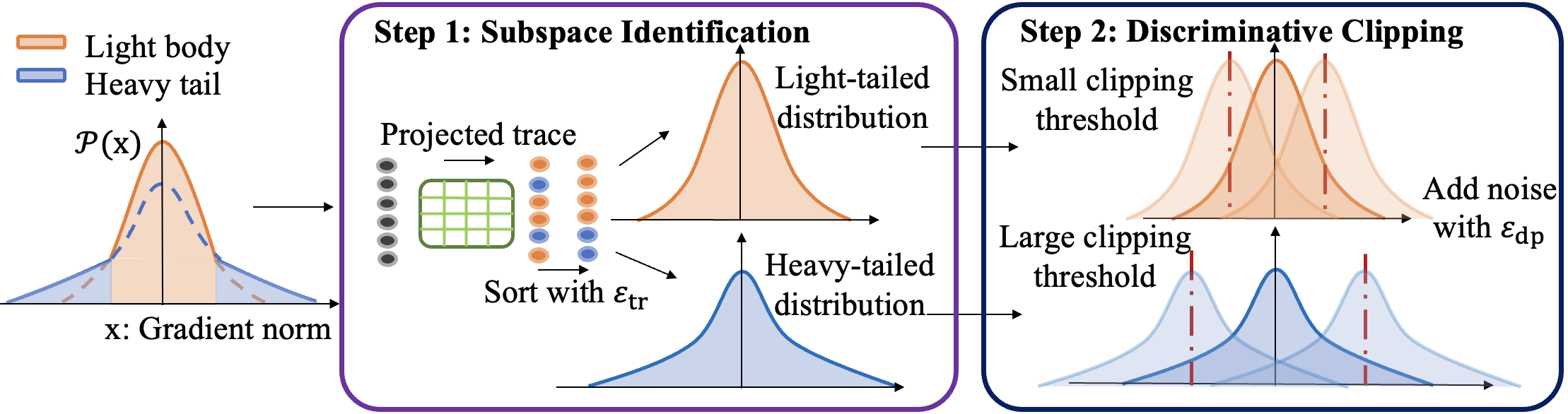
Figure 2: Overview of DC-DPSGD.

In the first step, we present a subspace identification technique to distinguish gradients. Given that the normalized gradients still retain directional information, which can be amplified when projected onto the subspace consistent with its underlying distribution, we can bypass the unbounded norm of heavy-tailed gradients and capture different responses of private gradients in the heavy-tailed subspace. In our approach, we construct projection matrix composed of random vectors following heavy-tailed sub-Weibull distributions ($\theta>\frac{1}{2}$). We then divide the gradients into the light body and heavy tail according to the projected traces $\lambda_{\mathrm{tr}}$, which are calculated from the sample second moment matrix. To satisfy differential privacy, noise with scale $\sigma_{\mathrm{tr}}$ is added.

In the second step, we utilize different clipping thresholds for the two parts and add DP noise with scale $\sigma_{\mathrm{dp}}$ based on the discriminative clipping thresholds for privacy preservation. For fairness, the total privacy budget allocated by DC-DPSGD to traces $\epsilon_{\mathrm{tr}}$ and gradients $\epsilon_{\mathrm{dp}}$ must be equal to the privacy budget $\epsilon$ in DPSGD variants, that is, $\epsilon=\epsilon_{\mathrm{tr}}+\epsilon_{\mathrm{dp}}$. Algorithm 1 presents the detailed steps of DC-DPSGD and Theorem 5.3 gives its privacy guarantee.

Theorem 5.1 (Privacy Guarantee).

There exist constants $m_{1}$ and $m_{2}$ such that for any $\epsilon_{\mathrm{tr}}\leq m_{1}q^{2}T$, $\epsilon_{\mathrm{dp}}\leq m_{1}q^{2}T$ and $\delta>0$, the noise multiplier $\sigma^{2}_{\mathrm{tr}}=\frac{m_{2}Tq^{2}\ln{\frac{1}{\delta}}}{\epsilon^{2}_{\mathrm{tr}}}$ and $\sigma^{2}_{\mathrm{dp}}=\frac{m_{2}Tq^{2}\ln{\frac{1}{\delta}}}{\epsilon^{2}_{\mathrm{dp}}}$ over the $T$ iterations, where $q=\frac{B}{n}$, and DC-DPSGD is $(\epsilon_{\mathrm{tr}}+\epsilon_{\mathrm{dp}},\delta)$-differentially private.

5.1 Subspace Closeness for Identification

As introduced above, we use subspace as an auxiliary tool to indirectly identify heavy-tailed gradients and reduce clipping loss. We construct the subspace $V_{k}V^{T}_{k}$ that is composed of $k$ random orthogonal unit vectors and we need to bound the gap between the empirical second moment and the population second moment, i.e. $\|V_{k}V^{T}_{k}-\mathbb{E}[V_{k}V^{T}_{k}]\|_{2}$. It is worth noting that we add extra noise in line 9 of Algorithm 1, as the publicly available traces need to be sorted to confirm the top-$p$ heavy-tailed gradients, which may expose intrinsic preferences of the samples. According to Ahlswede-Winter Inequality wainwright2019high , we analyze the error of subspace skewing in a high probability form.

Theorem 5.2 (Subspace Skewing for Identification).

Assume that the second moment matrix $M:=V_{k}V^{T}_{k}$ with $V^{T}_{k}V_{k}=\mathbb{I}$ approximates the population second moment matrix $\hat{M}:=\hat{V}_{k}\hat{V}^{T}_{k}=\mathbb{E}[V_{k}V^{T}_{k}]$, $\lambda_{\mathrm{tr}}:=\mathrm{tr}(V^{T}_{k}uu^{T}V_{k})$ and $\hat{\lambda}_{\mathrm{tr}}:=\mathrm{tr}(\hat{V}^{T}_{k}uu^{T}\hat{V}_{k})$, for any vector $u$ that satisfies $\|u\|_{2}=1$, $\zeta_{\mathrm{tr}}\sim\mathbb{N}(0,\sigma^{2}_{\mathrm{tr}}\mathbb{I})$ and $\delta\in(0,1)$, with probability $1-\delta_{m}-\delta$, we have

$$|\lambda_{\mathrm{tr}}-\hat{\lambda}_{\mathrm{tr}}+\zeta_{\mathrm{tr}}|\leq\frac{4\log{(2d/\delta_{m})}}{k}+\sigma_{\mathrm{tr}}\log^{\frac{1}{2}}(2/\delta).$$

Remark 5.1.

Because we have normalized per-sample gradient in advance, the upper bound of the trace for per-sample gradient is limited to 1. So, the sensitivity in differential privacy can be regarded as 1. In addition, since $\lambda_{\mathrm{tr}}$ is a constant, the scale $\sigma_{\mathrm{tr}}$ of noise added is small compared to the noise scale $\sigma^{2}_{\mathrm{dp}}$ added to gradients. In this case, the probability term $\log{(2d/\delta_{m})}/k$ dominates this boundary and decreases as $k$ increases, so the error is negligible when $k$ is large. Since $\lambda_{\mathrm{tr}}$ represents the total variance of the gradient in the $k$-dimensional subspace, we know from Theorem 5.2 that the upper bound of the error between this value and the variance of the actual distribution is finite. In other words, Theorem 5.2 indicates that we can accurately identify and classify gradients with a high probability $1-\delta^{\prime}_{m}$, where $\delta^{\prime}_{m}=\delta+\delta_{m}$.

Algorithm 1 Discriminative Clipping DPSGD with Subspace Identification

Input: Private batch size $B$, heavy-tailed ratio $p$, heavy-tailed clipping threshold $c_{1}$, light-tailed clipping threshold $c_{2}$, learning rate $\eta_{t}$ and subspace dimension $k$.

1:  Initialize $\mathbf{w}_{0}$ randomly.

2:  for $e\in E$ do

3:     Initialize $V_{t,k}$ to None.

4:     for $t\in T$ do

5:        Take a random batch $B$ with sampling ratio $B/n$ and $g_{t}(z_{i})=\nabla\ell(\mathbf{w}_{t},z_{i})$.

6:        Extract orthogonal vectors $[v_{1},...,v_{k}]$ from sub-Weibull distributions and construct projection subspace with $V_{t,k}V^{T}_{t,k}=\frac{1}{k}\sum^{k}_{i=1}v_{i}v^{T}_{i}$.

7:        Normalize per-sample gradient $\hat{g}_{t}(x_{i})=g_{t}(x_{i})/\|g_{t}(x_{i})\|$.

8:        Calculate the trace $\lambda_{i}$ of the projected second moment $V^{T}_{t,k}\hat{g}_{t}(x_{i})\hat{g}^{T}_{t}(x_{i})V_{t,k}$.

9:        Perturb traces with noise $\widetilde{\lambda}_{i}=\lambda_{i}+\mathbb{N}(0,\sigma^{2}_{\mathrm{tr}}\mathbb{I})$ and identify top-$p$ based on sorted $\widetilde{\lambda}_{i}$.

10:        Clip per-sample gradient and add noise. For heavy tail:  $\overline{g}_{t}(z^{\mathrm{tail}}_{i})=g_{t}(z^{\mathrm{tail}}_{i})/\mathrm{max}(1,\frac{\|g_{t}(z^{\mathrm{tail}}_{i})\|_{2}}{c_{1}})+\mathbb{N}(0,c_{1}^{2}\sigma^{2}_{\mathrm{dp}}\mathbb{I})$ For light body:  $\overline{g}_{t}(z^{\mathrm{body}}_{i})=g_{t}(z^{\mathrm{body}}_{i})/\mathrm{max}(1,\frac{\|g_{t}(z^{\mathrm{body}}_{i})\|_{2}}{c_{2}})+\mathbb{N}(0,c_{2}^{2}\sigma^{2}_{\mathrm{dp}}\mathbb{I})$

11:        Weighted average $\widetilde{g}_{t}=\frac{1}{B}\left(\sum^{pB}_{i=1}\overline{g}_{t}(z^{\mathrm{tail}}_{i})+\sum^{(1-p)B}_{i=1}\overline{g}_{t}(z^{\mathrm{body}}_{i})\right)$.

12:        Update $\mathbf{w}_{t+1}=\mathbf{w}_{t}-\eta_{t}\widetilde{g}_{t}$.

13:     end for

14:  end for

5.2 Convergence of Discriminative Clipping DPSGD

Next, we delve into the convergence analysis of DC-DPSGD based on the aforementioned clipping mechanism. Typically, the tail probability $\mathbb{P}(|x|>t)=\exp{(-I(t))}~{}\forall{t>0}$ of the sub-Weibull variables $x\sim subW(\theta,K)$ exhibits two different behaviors: 1) For small $t$ values, the tail rate capturing function $I(t)$ decays like a sub-Gaussian tail. 2) For $t$ greater than the normal convergence region, i.e., $t\geq t_{\mathrm{max}}$ is a large deviation region, its decay is slower than that of the normal distribution. Existing literature has studied the first region in the optimization analysis for DPSGD zhou2020bypassing ; bu2024automatic ; yang2022normalized ; xia2023differentially ; cheng2022differentially ; xiao2023theory ; sha2023pcdp , but they overlook the heavy-tailed behavior for the second region. In our work, we not only investigate the optimization performance of one specific region, but also combine the two tailed-rate regions with our proposed discrimination clipping mechanism. To construct a comprehensive optimization framework under heavy-tailed assumptions, we generalize the sharp heavy-tailed concentration bakhshizadeh2023sharp and sub-Weibull Freedman inequality madden2020high to truncated versions. Consequently, we have the following theorem:

Theorem 5.3 (Convergence of Discriminative Clipping DPSGD).

Under Assumptions 3.1, 3.2 and 3.3, let $\mathbf{w}_{t}$ be the iterate produced by DC-DPSGD and $\eta_{t}=\frac{1}{\sqrt{T}}$. Define $\hat{\log}(T/\delta)=\log^{\max(0,\theta-1)}(T/\delta)$, $\lambda_{\mathrm{max}}=\frac{\mu I(\lambda)}{\lambda}aK^{2}$, $a=2$ if $\theta=\frac{1}{2}$, $a=(4\theta)^{2\theta}e^{2}$ if $\theta\in(\frac{1}{2},1]$, and $a=(2^{2\theta+1}+2)\Gamma(2\theta+1)+\frac{2^{3\theta}\Gamma(3\theta+1)}{3}$ if $\theta>1$, for any $\delta\in(0,1)$, then we have:

1. For the case $0\leq\lambda_{\mathrm{tr}}\leq\lambda_{\mathrm{max}}$, suppose that $T=\max{\big{(}m_{2}eB^{2}\log(1/\delta),\frac{n\epsilon}{\sqrt{d\log(1/\delta)}}\big{)}}$ and $c=\max{\big{(}2\sqrt{2a}K\log^{\frac{1}{2}}({\sqrt{T}}),33\sqrt{2a}K\log^{\frac{1}{2}}(2/\delta)\big{)}}$, with probability $1-\delta$,

   $$\frac{1}{T}\sum^{T}_{t=1}\min\big{\{}\|\nabla L_{S}(\mathbf{w}_{t})\|_{2},\|\nabla L_{S}(\mathbf{w}_{t})\|^{2}_{2}\big{\}}\leq\mathbb{O}\left(\frac{d^{\frac{1}{4}}\log^{\frac{5}{4}}(T/\delta)\log(\sqrt{T})}{(n\epsilon)^{\frac{1}{2}}}\right).$$

2. For the case $\lambda_{\mathrm{tr}}\geq\lambda_{\mathrm{max}}$, suppose that $T=\max{\big{(}m_{2}eB^{2}\log(1/\delta),\frac{n\epsilon}{\sqrt{d\log(1/\delta)}}\big{)}}$ and $c=\max{\big{(}4^{\theta}2K\log^{\theta}({\sqrt{T}}),4^{\theta}33K\log^{\theta}(2/\delta)\big{)}}$, with probability $1-\delta$,

   $$\frac{1}{T}\sum^{T}_{t=1}\min\big{\{}\|\nabla L_{S}(\mathbf{w}_{t})\|_{2},\|\nabla L_{S}(\mathbf{w}_{t})\|^{2}_{2}\big{\}}\leq\mathbb{O}\left(\frac{d^{\frac{1}{4}}\log^{\frac{5}{4}}(T/\delta)\hat{\log}(T/\delta)\log^{2\theta}(\sqrt{T})}{(n\epsilon)^{\frac{1}{2}}}\right).$$

Remark 5.2.

From Theorem 5.3, we can infer that when gradients fall into the first light body region, i.e. $0\leq\lambda\leq\lambda_{\mathrm{max}}$, our results no longer contain the heavy-tailed index $\theta$. This implies that in this region, the optimization performance of the algorithm is not directly affected by the heavy-tailed assumption and always converges according to the light-tailed sub-Gaussian rate. However, when gradients are classified into the second heavy-tailed region, i.e. $\lambda\geq\lambda_{\mathrm{max}}$, the behavior of convergence in this part will remain the same as that of classic DPSGD, becoming deteriorated with the increase of $\theta$. Specifically, the optimization performance in the first region is actually a transformation of the second region when $\theta=\frac{1}{2}$. In the first light body part, our guidance for the clipping threshold depends on the logarithmic factor $\log^{1/2}$, but in the second heavy-tailed region, our theoretical clipping threshold increases with the heavy-tailed index $\log^{\theta}$. For $\lambda_{\mathrm{max}}$, it is correlated with the population variance of the underlying distribution in Assumption 3.1 bakhshizadeh2023sharp , and we empirically use the trace of the second moment to approximate the total variance of the gradients in the subspace, where the approximation error has been bounded in Theorem 5.2. In summary, unlike existing optimization results on the heavy-tailed assumption that entirely rely on the heavy-tailed index li2022high ; madden2020high , our DC-DPSGD bounds are partially free from the dependence on heavy tails and can provide theoretical guidance on large clipping thresholds.

5.3 Uniform Bound for Heavy-tailed DC-DPSGD

According to Algorithm 1 and Theorem 5.2, we note that the premise of discriminative clipping relies on the classification of gradients by the subspace. However, in practice, this step incurs errors and losses, leading to a misalignment between Theorem 5.3 and the algorithm. Considering that the accuracy of subspace identification holds with high probability at $1-\delta^{\prime}_{m}$, we need to re-analyze the convergence associated with partitioning regions in DC-DPSGD. Therefore, in this section, we will merge Theorems 5.2 and  5.3 to derive the final bound for Algorithm 1.

Theorem 5.4 (Uniform Bound for DC-DPSGD).

Under Assumptions 3.1, 3.2 and 3.3, combining Theorem 5.2 and Theorem 5.3, for any $\delta^{\prime}\in(0,1)$, with probability $1-\delta^{\prime}$ and $\mathcal{C}_{\mathrm{u}}:=\sum^{T}_{t=1}\min\{\|\nabla\hat{L}_{S}(\mathbf{w}_{t})\|^{2}_{2},\|\nabla\hat{L}_{S}(\mathbf{w}_{t})\|_{2}\}$, we have

$$\mathcal{C}_{\mathrm{u}} \leq p*\mathbb{O}\left(\frac{d^{\frac{1}{4}}\log^{\frac{5}{4}}(T/\delta)\hat{\log}(T/\delta)\log^{2\theta}(\sqrt{T})}{(n\epsilon)^{\frac{1}{2}}}\right)+(1-p)*\mathbb{O}\left(\frac{d^{\frac{1}{4}}\log^{\frac{5}{4}}(T/\delta)\log(\sqrt{T})}{(n\epsilon)^{\frac{1}{2}}}\right),$$

where $\delta^{\prime}=\delta^{\prime}_{m}+\delta$, $\hat{\log}(T/\delta)=\log^{\max(0,\theta-1)}(T/\delta)$ and $p$ is ratio of heavy-tailed gradients.

Remark 5.3.

Theorem 5.4 states that when the proportion of the tail region is $p$, the optimization performance of DC-DPSGD with subspace identification is composed of $p$-weighted average bounds, where the heavy-tailed convergence rate merely accounts for a portion of $p$, with the rest made up of the light rate. Therefore, our bound minimizes the dependency on $\theta$ from $\hat{\log}(T/\delta)\log^{2\theta}(\sqrt{T})$ to $\log(\sqrt{T})$ with percentage $(1-p)*(1-\delta^{\prime})$, which is tighter than DPSGD. According to the statistical properties wainwright2019high ; vershynin2018high , around 5% -10% data points will fall to the tail, that is, $p\in[0.05,0.1]$. The probability term $\delta^{\prime}$ includes both $\delta^{\prime}_{m}$ and $\delta$, with $\delta^{\prime}_{m}$ being the error of subspace identification and $\delta$ being the convergence probability of DC-DPSGD.

6 Experiments

6.1 Experimental Setup

We use four real-world datasets in the experiments, including MNIST, FMNIST, CIFAR10, and ImageNette (a subset of ImageNet deng2009imagenet ). We further utilize two heavy-tailed versions: namely CIFAR10-HT cao2019learning  (a heavy-tailed version of CIFAR10) and ImageNette-HT (modified on park2021influence ), to evaluate the performance under heavy tail assumption. For MNIST and FMNIST, we use a two-layer CNN with batch size $B=128$. For CIFAR10 and CIFAR10-HT, we take $B=256$ and fine-tune on model SimCLRv2 pre-trained by unlabeled ImageNet and ResNeXt-29 pre-trained by CIFAR100 tramer2020differentially with a linear classifier, respectively. For ImageNette and ImageNette-HT, we adopt the same settings bu2024automatic and ResNet9 without pre-train.

We compare DC-DPSGD with three differentially private baselines: DPSGD with Abadi’s clipping abadi2016deep , Auto-S/NSGD bu2024automatic ; yang2022normalized , DP-PSAC xia2023differentially , and a non-private baseline: non-DP ($\epsilon=\infty$). In addition, we set $c_{2}=0.1$ and $\eta=0.1$ for MNIST and FMNIST. For CIFAR10 tasks, we set $c_{2}=0.01$ and $\eta=10$, and let $c_{2}=0.15$, $\eta=0.0001$ and $B=1000$ on ImageNette tasks. The large clipping threshold is set as $c_{1}=10*c_{2}$. We implement per-sample clipping in private SGD by BackPACK dangel2020backpack and allocate privacy budget fairly according to $\epsilon=\epsilon_{\mathrm{dp}}+\epsilon_{\mathrm{tr}}$.

6.2 Effectiveness Evaluation

Table 2 summarizes the test accuracy of DC-DPSGD and baselines. We can observe that, on normal datasets, DC-DPSGD outperforms DPSGD, Auto-S, and DP-PSAC by up to 4.57%, 5.42%, and 4.99%, respectively. While on heavy-tailed datasets, the corresponding improvements are 8.34%, 9.72%, and 9.55%. The reason is that our approach places greater emphasis on the clipping weight of heavy-tailed gradients, thereby preserving more information about heavy-tailed gradients and improving accuracy. Moreover, we demonstrate the trajectories of training accuracy in Figure 4, indicating that the optimization performance of DC-DPSGD is superior to existing clipping mechanisms.

Table 2: Test accuracy of baselines and DC-DPSGD.

Dataset	DP ($\epsilon,\delta$)	Accuracy %
		DPSGD abadi2016deep	Auto-S bu2024automatic ; yang2022normalized	DP-PSAC xia2023differentially	Ours	non-DP
MNIST	(8,$1e^{-5}$)	97.65$\pm$0.09	97.55$\pm$0.16	97.67$\pm$0.06	98.72$\pm$0.02	99.10$\pm$0.02
FMNIST	(8,$1e^{-5}$)	83.23$\pm$0.10	82.38$\pm$0.15	82.81$\pm$0.18	87.80$\pm$0.47	89.95$\pm$0.32
CIFAR10	(8,$1e^{-5}$)	93.31$\pm$0.01	93.28$\pm$0.06	93.30$\pm$0.03	94.05$\pm$0.11	94.62$\pm$0.03
CIFAR10	(4,$1e^{-5}$)	93.06$\pm$0.09	93.08$\pm$0.06	93.11$\pm$0.08	93.42$\pm$0.14	94.62$\pm$0.03
ImageNette	(8,$1e^{-4}$)	66.81$\pm$0.42	65.57$\pm$0.85	65.68$\pm$1.71	69.29$\pm$0.19	71.67$\pm$0.49
CIFAR10-HT	(8,$1e^{-5}$)	57.98$\pm$0.59	58.30$\pm$0.61	57.99$\pm$0.58	62.57$\pm$1.03	71.74$\pm$0.65
ImageNette-HT	(8,$1e^{-4}$)	25.36$\pm$1.71	23.98$\pm$2.00	24.15$\pm$1.99	33.70$\pm$0.91	39.91$\pm$1.46

We then evaluate the effects of three parameters on test accuracy, including the subspace-$k$, the allocation of privacy budget $\epsilon$, and the heavy tail index sub-Weibull-$\theta$. The results are shown in Table 3. We can see that the test accuracy increases with the value of $k$, which aligns with the theory that the trace error is related to $\mathbb{O}(1/k)$ and has a small impact on the results. For the allocation of privacy budget between subspace identification and privacy oracle, we find that allocation biased towards moderate or $\epsilon_{\mathrm{tr}}$ is better due to the high dimensionality of gradients. For subspace distribution, since the ‘HT’ dataset is extracted through sub-Exponential distributions, the gradient exhibits a heavier tail phenomenon in networks. Therefore, the accuracy increases as $\theta$ becomes larger.

Table 3: Effects of parameters on test accuracy.

Dataset	Subspace-$k$				$\epsilon_{\mathrm{tr}}$ + $\epsilon_{\mathrm{dp}}$			sub-Weibull-$\theta$
	None	100	150	200	2+6	4+4	6+2	1/2	1	2
CIFAR10	93.07	93.82	93.96	94.05	93.92	94.05	93.37	93.88	93.99	94.05
CIFAR10-HT	57.27	61.60	62.48	62.57	62.54	62.57	60.07	61.58	62.28	62.57

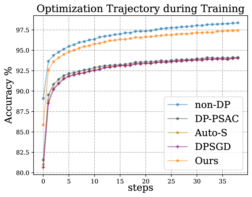
Figure 3: Optimization performance during CIFAR10 Training.

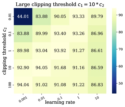
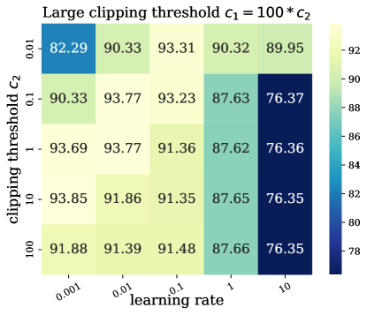
Figure 4: Test accuracy heatmap on CIFAR10 with $c_{1}$, $c_{2}$ and $\eta$.

6.3 Guidance for Large Clipping Threshold

Based on the theoretical analysis in Theorem 5.3 and experimental results in Figure 4, we can provide a recommended interval of clipping threshold for DC-DPSGD. Taking CIFAR-10 as an example, where $\delta=1e^{-5}$ and $\eta/B=0.04$, we combine the empirical $\theta\approx 2$ with the theoretical guidance in gurbuzbalaban2021heavy . Consequently, we obtain $c_{1}=\mathbb{O}(\log^{\theta}(1/\delta))$ is $\sqrt{125}$ times larger than $c_{2}=\mathbb{O}(\log^{1/2}(1/\delta))$, that is, $c_{1}=\log^{3/2}(1/\delta)c_{2}$ and then $c_{1}\approx 10c_{2}$.

7 Conclusion

In this paper, we propose a novel approach DC-DPSGD under the heavy-tailed assumption, which effectively reduces extra clipping loss in the heavy-tailed region. We rigorously analyze the high-probability bound of the classic heavy-tailed DPSGD under non-convex conditions and obtain results matching the expectation bounds. Furthermore, we characterize the weighted average optimization performance of DC-DPSGD. Extensive experiments on four real-world datasets validate that DC-DPSGD outperforms three state-of-the-art clipping mechanisms for heavy-tailed gradients.

Appendix

Appendix A Preliminaries

A random variable $X$ called a sub-Weibull random variable with tail parameter $\theta$ and scale factor $K$, which is denoted by $X\sim subW(\theta,K)$. We next introduce the equivalent properties and theoretical tools of sub-Weibull distributions.

A.1 Properties

Definition A.1 (Sub-Weibull Equivalent Properties vladimirova2020sub ).

Let $X$ be a random variable and $\theta\geq 0$, and there exists some constant $K_{1},K_{2},K_{3},K_{4}$ depending on $\theta$. Then the following characterizations are equivalent:

1. The tails of $X$ satisfy

   $$\exists K_{1}>0~{}\text{such that}~{}\mathbb{P}(|X|>t)\leq 2\mathrm{exp}(-(t/K_{1})^{\frac{1}{\theta}}),\forall t>0.$$

2. The moments of $X$ satisfy

   $$\exists K_{2}>0~{}\text{such that}~{}\|X\|_{p}\leq K_{2}p^{\theta},\forall k\geq 1.$$

3. The moment generating function (MGF) of $|X|^{\frac{1}{\theta}}$ satisfies

   $$\exists K_{3}>0~{}\text{such that}~{}\mathbb{E}[\mathrm{exp}((\lambda|X|)^{\frac{1}{\theta}})]\leq\mathrm{exp}((\lambda K_{3})^{\frac{1}{\theta}}),\forall\lambda\in(0,1/K_{3}).$$

4. The MGF of $|X|^{\frac{1}{\theta}}$ is bounded at some point,

   $$\exists K_{4}>0~{}\text{such that}~{}\mathbb{E}[\mathrm{exp}((|X|/K_{4})^{\frac{1}{\theta}})]\leq 2.$$

Fact A.1.

For any $V_{k}\in\mathbb{R}^{d\times k}$, $\mathrm{tr}(V^{T}_{k}\nabla\ell\nabla\ell^{T}V_{k})=\|V^{T}_{k}\nabla\ell\|^{2}_{2}$. Moreover, if the condition $V^{T}_{k}V_{k}=\mathbb{I}$ holds, then $\|V^{T}_{k}\nabla\ell\|^{2}_{2}=\|V_{k}V^{T}_{k}\nabla\ell\|^{2}_{2}$.

A.2 Theoretical tools

Based on the properties of sub-Weibull variables, we have the following high probability bounds and concentration inequalities for heavier tails as theoretical tools. Besides, We define $l_{p}$ norm as $\|\|_{p}$, for any $p\geq 1$.

Lemma A.1.

Let a variable $X\sim subW(\theta,K)$, for any $\delta\in(0,1)$, then with probability $(1-\delta)$ we have

$$|X|\leq K\log^{\theta}{(2/\delta)}.$$

Proof.

Let $K_{1}=K$ in Definition A.1, and take $t=K\log^{\theta}{(2/\delta)}$, then the inequality holds with probability $1-\delta$. ∎

Lemma A.2 (vladimirova2020sub ; madden2020high ).

Let $X_{1},...,X_{n}$ are $subW(\theta,K_{i})$ random variables with scale parameters $K_{1},...K_{n}$. $\forall t\geq 0$, we have

$$\mathbb{P}(|\sum^{n}_{i=1}X_{i}|\geq t)\leq 2\mathrm{exp}(-(\frac{t}{g(\theta)\sum^{n}_{i=1}K_{i}})^{\frac{1}{\theta}})$$

where $g(\theta)=(4e)^{\theta}$ for $\theta\leq 1$ and $g(\theta)=2(2e\theta)^{\theta}$ for $\theta\geq 1$.

Lemma A.3 (Sub-Weibull Freedman Inequality madden2020high ).

Let $(\Omega,\mathcal{F},(\mathcal{F}_{i}),\mathbb{P})$ be a filtered probability space. Let $(\xi_{i})$ and $(K_{i})$ be adapted to $(\mathcal{F}_{i})$. Let $n\in\mathbb{N}$, then $\forall i\in[n]$, assume $K_{i-1}\geq 0$, $\mathbb{E}[\xi_{i}|\mathcal{F}_{i-1}]=0$, and $\mathbb{E}[\mathrm{exp}((|\xi_{i}|/K_{i-1})^{\frac{1}{\theta}})|\mathcal{F}_{i-1}]\leq 2$ where $\theta\geq 1/2.$ If $\theta>1/2$, assume there exists $(m_{i})$ such that $K_{i-1}\leq m_{i}$.

if $\theta=1/2$, let $a=2$, then $\forall x,\beta\geq 0$, $\alpha>0$, and $\lambda\in[0,\frac{1}{2\alpha}]$,

$$\mathbb{P}\left(\bigcup_{k\in[n]}\Big{\{}\sum^{k}_{i=1}\xi_{i}\geq x~{}\mathrm{and}~{}\sum^{k}_{i=1}aK^{2}_{i-1}\leq\alpha\sum^{k}_{i=1}\xi_{i}+\beta\Big{\}}\right)\leq\mathrm{exp}(-\lambda x+2\lambda^{2}\beta),$$ (3)

and $\forall x,\beta,\lambda\geq 0$,

$$\mathbb{P}\left(\bigcup_{k\in[n]}\Big{\{}\sum^{k}_{i=1}\xi_{i}\geq x~{}\mathrm{and}~{}\sum^{k}_{i=1}aK^{2}_{i-1}\leq\beta\Big{\}}\right)\leq\mathrm{exp}(-\lambda x+\frac{\lambda^{2}}{2}\beta).$$ (4)

If $\theta\in(\frac{1}{2},1]$, let $a=(4\theta)^{2\theta}e^{2}$ and $b=(4\theta)^{\theta}e$. $\forall x,\beta\geq 0$, and $\alpha\geq b\mathrm{max}_{i\in[n]}m_{i}$, and $\lambda\in[0,\frac{1}{2\alpha}]$,

$$\mathbb{P}\left(\bigcup_{k\in[n]}\Big{\{}\sum^{k}_{i=1}\xi_{i}\geq x~{}\mathrm{and}~{}\sum^{k}_{i=1}aK^{2}_{i-1}\leq\alpha\sum^{k}_{i=1}\xi_{i}+\beta\Big{\}}\right)\leq\mathrm{exp}(-\lambda x+2\lambda^{2}\beta),$$ (5)

and $\forall x,\beta\geq 0$, and $\lambda\in[0,\frac{1}{b\mathrm{max}_{i\in[n]}m_{i}}]$,

$$\mathbb{P}\left(\bigcup_{k\in[n]}\Big{\{}\sum^{k}_{i=1}\xi_{i}\geq x~{}\mathrm{and}~{}\sum^{k}_{i=1}aK^{2}_{i-1}\leq\beta\Big{\}}\right)\leq\mathrm{exp}(-\lambda x+\frac{\lambda^{2}}{2}\beta).$$ (6)

If $\theta>1$, let $\delta\in(0,1)$. Let $a=(2^{2\theta+1}+2)\Gamma(2\theta+1)+2^{3\theta}\Gamma(3\theta+1)/3$ and $b=2\log{n/\delta}^{\theta-1}$, where $\Gamma(x)=\int^{\infty}_{0}t^{x-1}e^{-t}dt$. $\forall x,\beta\geq 0$, $\alpha\geq b\mathrm{max}_{i\in[n]}m_{i}$, and $\lambda\in[0,\frac{1}{2\alpha}]$,

$$\mathbb{P}\left(\bigcup_{k\in[n]}\Big{\{}\sum^{k}_{i=1}\xi_{i}\geq x~{}\mathrm{and}~{}\sum^{k}_{i=1}aK^{2}_{i-1}\leq\alpha\sum^{k}_{i=1}\xi_{i}+\beta\Big{\}}\right)\leq\mathrm{exp}(-\lambda x+2\lambda^{2}\beta)+2\delta,$$ (7)

and $\forall x,\beta\geq 0$, and $\lambda\in[0,\frac{1}{b\mathrm{max}_{i\in[n]}m_{i}}]$,

$$\mathbb{P}\left(\bigcup_{k\in[n]}\Big{\{}\sum^{k}_{i=1}\xi_{i}\geq x~{}\mathrm{and}~{}\sum^{k}_{i=1}aK^{2}_{i-1}\leq\beta\Big{\}}\right)\leq\mathrm{exp}(-\lambda x+\frac{\lambda^{2}}{2}\beta)+2\delta.$$ (8)

Lemma A.4 (zhang2005data ).

Let $z_{1},...,z_{n}$ be a sequence of randoms variables such that $z_{k}$ may depend the previous variables $z_{1},...,z_{k-1}$ for all $k=1,...,n$. Consider a sequence of functionals $\xi_{k}(z_{1},...,z_{k})$, $k=1,...,n$. Let $\sigma^{2}_{n}=\sum^{n}_{k=1}\mathbb{E}_{z_{k}}[(\xi_{k}-\mathbb{E}_{z_{k}}[\xi_{k}])^{2}]$ be the conditional variance. Assume $|\xi_{k}-\mathbb{E}_{z_{k}}[\xi_{k}]|\leq b$ for each $k$. Let $\rho\in(0,1]$ and $\delta\in(0,1)$. With probability at least $1-\delta$ we have

$$\sum^{n}_{k=1}\xi_{k}-\sum^{n}_{k=1}\mathbb{E}_{z_{k}}[\xi_{k}]\leq\frac{\rho\sigma^{2}_{n}}{b}+\frac{b\log{\frac{1}{\delta}}}{\rho}.$$ (9)

Lemma A.5 (cutkosky2020momentum ).

For any vector $\mathbf{g}\in\mathbb{R}^{d}$, $\langle\mathbf{g}/\|\mathbf{g}\|_{2},\nabla L_{S}(\mathbf{w})\rangle\geq\frac{\|\nabla L_{S}(\mathbf{w})\|_{2}}{3}-\frac{8\|\mathbf{g}-L_{S}(\mathbf{w})\|_{2}}{3}$.

Lemma A.6 (madden2020high ).

If $X\sim subW(\theta,K)$, then $\mathbb{E}[|X^{p}|]\leq 2\Gamma(p\theta+1)K^{p}~{}\forall p>0$. In particular, $\mathbb{E}[X^{2}]\leq 2\Gamma(2\theta+1)K^{2}$.

Lemma A.7 (bakhshizadeh2023sharp ).

Suppose $X_{1},...,X_{m}\overset{d}{=}X$ are independent and identically distributed random variables whose right tails are captured by an increasing and continuous function $I:\mathbb{R}\rightarrow\mathbb{R}^{\geq 0}$ with the property $I(t)=\mathbb{O}(t)$ as $t\rightarrow\infty$. Let $X^{L}=X\mathbb{I}(X\leq L)$, $S_{m}=\sum^{m}_{i=1}X_{i}$ and $Z^{L}:=X^{L}-\mathbb{E}[X]$. Define $t_{\mathrm{max}}(\mu):=\mathrm{sup}\{t\geq 0:t\leq\mu v(mt,\mu)\frac{I(mt)}{mt}\}$, then

$$\mathbb{P}(S_{m}-\mathbb{E}[S_{m}]>mt)\leq\left\{\begin{array}[]{ll}\mathrm{exp}(-c_{t}\mu I(mt))+m\mathrm{exp}(-I(mt)),&\text{if }t\geq t_{\mathrm{max}}(\mu),\\ \\ \displaystyle\mathrm{exp}(-\frac{mt^{2}}{2v(mt_{\mathrm{max}}(\mu),\mu)})+m\mathrm{exp}(-\frac{mt^{2}_{\mathrm{max}}(\mu)}{\mu v(mt_{\mathrm{max}}(\mu),\mu)}),&\text{if }0\leq t\leq t_{\mathrm{max}}(\mu),\end{array}\right.$$ (13)

where $c_{t}=1-\frac{\mu v(mt,\mu)I(mt)}{2mt^{2}}$ and $v(L,\mu)=\mathbb{E}\big{[}(Z^{L})^{2}\mathbb{I}(Z^{L}\leq 0)+(Z^{L})^{2}~{}\mathrm{exp}(\mu\frac{I(L)}{L}Z^{L})\mathbb{I}(Z^{L}>0)\big{]},\forall\beta\in(0,1]$.

Lemma A.8 (bakhshizadeh2023sharp ).

Consider the same settings as the ones in Lemma A.7. Assume $\mathbb{E}[X_{i}]=0$, then $\forall t\geq 0$ we have

$$\mathbb{P}(S_{m}>mt)\leq\mathrm{exp}(-\frac{mt^{2}}{2v(mt,\mu)})+\mathrm{exp}(-\mu\max\{c_{t},\frac{1}{2}\}I(mt))+m\mathrm{exp}(-I(mt)).$$ (14)

Lemma A.9 (Ahlswede-Winter Inequality wainwright2019high ).

Let $Y$ be a random, symmetric, positive semi-definite $d×d$ matrix such that $\|\mathbb{E}[Y]\|_{2}\leq 1$. Suppose $\|Y\|_{2}\leq R$ for some fixed scalar $R\geq 1$. Let $Y_{1},...,Y_{m}$ be independent copies of $Y$ (i.e., independently sampled matrix with the same distribution as $Y$). For any $\mu\in(0,1)$, we have

$$\mathbb{P}(\|\frac{1}{m}\sum_{i=1}^{m}Y_{i}-\mathbb{E}[Y_{i}]\|_{2}>\mu)\leq 2d\cdot\text{exp}(-m\mu^{2}/4R).$$

Appendix B Convergence of Heavy-tailed DPSGD

Algorithm 2 Outline of DPSGD abadi2016deep

Input: Samples $n$, Private batch size $B$, clipping threshold $c$, learning rate $\eta_{t}$ and noise scale $\sigma$.

1:  Initialize $\mathbf{w}_{0}$ randomly.

2:  for $e\in E$ do

3:     for $t\in T$ do

4:        Take a random batch $B$ with sampling ratio $B/n$ and $g_{t}(z_{i})=\nabla\ell(\mathbf{w}_{t},z_{i})$.

5:        Clip per-sample gradient. $\overline{g}_{t}(z_{i})=g_{t}(z_{i})/\mathrm{max}(1,\frac{\|g_{t}(z_{i})\|_{2}}{c})$ .

6:        Add noise and average.$\widetilde{g}_{t}=\frac{1}{B}(\sum^{B}_{i=1}\overline{g}_{t}(z_{i})+\mathbb{N}(0,c^{2}\sigma^{2}\mathbb{I}))$.

7:        Update $\mathbf{w}_{t+1}=\mathbf{w}_{t}-\eta_{t}\widetilde{g}_{t}$.

8:     end for

9:  end for

Theorem B.1 (Convergence of Heavy-tailed DPSGD).

Under Assumption A.1, let $\mathbf{w}_{t}$ be the iterate produced by Algorithm 2-DPSGD and $\eta_{t}=\frac{1}{\sqrt{T}}$. If $\theta=\frac{1}{2}$ and $19K\log^{\theta}(2/\delta)\leq 12\sqrt{e}\sigma_{\mathrm{dp}}\log^{\frac{1}{2}}(2/\delta)$, then $T=\max{\big{(}m_{2}eB^{2}\log(1/\delta),\frac{n\epsilon}{\sqrt{d\log(1/\delta)}}\big{)}}$ and $c=\max{\big{(}4K\log^{\theta}({\sqrt{T}}),27\sqrt{e}\sigma_{\mathrm{dp}}\log^{\frac{1}{2}}(2/\delta)\big{)}}$. If $\theta=\frac{1}{2}$ and $19K\log^{\theta}(2/\delta)\geq 12\sqrt{e}\sigma_{\mathrm{dp}}\log^{\frac{1}{2}}(2/\delta)$, then $T=\frac{n\epsilon}{\sqrt{d\log(1/\delta)}}$ and $c=\max{\big{(}4K\log^{\theta}({\sqrt{T}}),39K\log^{\frac{1}{2}}(2/\delta)\big{)}}$. If $\theta>\frac{1}{2}$, then $T=\frac{n\epsilon}{\sqrt{d\log(1/\delta)}}$ and $c=\max{\big{(}4K\log^{\theta}({\sqrt{T}}),20K\log^{\theta}(2/\delta)\big{)}}$. For any $\delta\in(0,1)$, with probability $1-\delta$, we have

$$\frac{1}{T}\sum^{T}_{t=1}\min\big{\{}\|\nabla L_{S}(\mathbf{w}_{t})\|_{2},\|\nabla L_{S}(\mathbf{w}_{t})\|^{2}_{2}\big{\}}\leq\mathbb{O}\left(\frac{d^{\frac{1}{4}}\log^{\frac{5}{4}}(T/\delta)\hat{\log}(T/\delta)\log^{2\theta}(\sqrt{T})}{(n\epsilon)^{\frac{1}{2}}}\right),$$

where $\hat{\log}(T/\delta)=\log^{\max(0,\theta-1)}(T/\delta)$.

Proof.

We consider two cases: $L_{S}(\mathbf{w}_{t})\leq c/2$ and $L_{S}(\mathbf{w}_{t})\geq c/2$.

We first consider the case $\nabla L_{S}(\mathbf{w}_{t})\leq c/2$ with Assumption 3.2.

$$L_{S}(\mathbf{w}_{t+1})-L_{S}(\mathbf{w}_{t})\leq\langle\mathbf{w}_{t+1}-\mathbf{w}_{t},\nabla L_{S}(\mathbf{w}_{t})\rangle+\frac{1}{2}\beta\|\mathbf{w}_{t+1}-\mathbf{w}_{t}\|^{2}$$ (15)

$$\leq-\eta_{t}\langle\overline{\mathbf{g}}_{t}+\mathbf{\zeta}_{t},\nabla L_{S}(\mathbf{w}_{t})\rangle+\frac{1}{2}\beta\eta^{2}_{t}\|\overline{\mathbf{g}}_{t}+\mathbf{\zeta}_{t}\|^{2}$$

$$=-\eta_{t}\langle\overline{\mathbf{g}}_{t}-\mathbb{E}_{t}[\overline{\mathbf{g}}_{t}]+\mathbb{E}_{t}[\overline{\mathbf{g}}_{t}]-\nabla L_{S}(\mathbf{w}_{t}),\nabla L_{S}(\mathbf{w}_{t})\rangle-\eta_{t}\langle\mathbf{\zeta}_{t},\nabla L_{S}(\mathbf{w}_{t})\rangle$$

$$-\eta_{t}\|\nabla L_{S}(\mathbf{w}_{t})\|^{2}+\frac{1}{2}\beta\eta^{2}_{t}\|\overline{\mathbf{g}}_{t}\|^{2}+\frac{1}{2}\beta\eta^{2}_{t}\|\mathbf{\zeta}_{t}\|^{2}+\beta\eta^{2}_{t}\langle\overline{\mathbf{g}}_{t},\mathbf{\zeta}_{t}\rangle$$

$$=-\eta_{t}\langle\overline{\mathbf{g}}_{t}-\mathbb{E}_{t}[\overline{\mathbf{g}}_{t}],\nabla L_{S}(\mathbf{w}_{t})\rangle-\eta_{t}\langle\mathbb{E}_{t}[\overline{\mathbf{g}}_{t}]-\nabla L_{S}(\mathbf{w}_{t}),\nabla L_{S}(\mathbf{w}_{t})\rangle-\eta_{t}\langle\mathbf{\zeta}_{t},\nabla L_{S}(\mathbf{w}_{t})\rangle$$

$$-\eta_{t}\|\nabla L_{S}(\mathbf{w}_{t})\|^{2}+\frac{1}{2}\beta\eta^{2}_{t}\|\overline{\mathbf{g}}_{t}\|^{2}+\frac{1}{2}\beta\eta^{2}_{t}\|\mathbf{\zeta}_{t}\|^{2}+\beta\eta^{2}_{t}\langle\overline{\mathbf{g}}_{t},\mathbf{\zeta}_{t}\rangle$$

Considering all $T$ iterations, we get

$$\sum^{T}_{t=1}\eta_{t}\|\nabla L_{S}(\mathbf{w}_{t})\|^{2}\leq L_{S}(\mathbf{w}_{1})-L_{S}(\mathbf{w}_{S})+\sum^{T}_{t=1}\frac{1}{2}\beta\eta^{2}_{t}c^{2}+\underbrace{\sum^{T}_{t=1}\frac{1}{2}\beta\eta^{2}_{t}\|\mathbf{\zeta}_{t}\|^{2}}_{\mathrm{E}.1}+\underbrace{\sum^{T}_{t=1}\beta\eta^{2}_{t}\langle\overline{\mathbf{g}}_{t},\mathbf{\zeta}_{t}\rangle}_{\mathrm{E}.2}$$

$$-\underbrace{\sum^{T}_{t=1}\eta_{t}\langle\mathbf{\zeta}_{t},\nabla L_{S}(\mathbf{w}_{t})\rangle}_{\mathrm{E}.3}-\underbrace{\sum^{T}_{t=1}\eta_{t}\langle\overline{\mathbf{g}}_{t}-\mathbb{E}_{t}[\overline{\mathbf{g}}_{t}],\nabla L_{S}(\mathbf{w}_{t})\rangle}_{\mathrm{E}.4}-\underbrace{\sum^{T}_{t=1}\eta_{t}\langle\mathbb{E}_{t}[\overline{\mathbf{g}}_{t}]-\nabla L_{S}(\mathbf{w}_{t}),\nabla L_{S}(\mathbf{w}_{t})\rangle}_{\mathrm{E}.5}$$ (16)

For E.1, E.2 and E.3, since $\zeta_{t}\sim\mathbb{N}(0,c^{2}\sigma^{2}_{\mathrm{dp}}\mathbb{I}_{d})$, we set $\sigma^{2}_{\mathrm{dp}}=m_{2}\frac{TdB^{2}\log(1/\delta)}{n^{2}\epsilon^{2}}$ for simplicity, with sub-Gaussian properties A.1 and Lemma A.2, with probability at least $1-\delta$, and we have

$$\sum^{T}_{t=1}\frac{1}{2}\beta\eta^{2}_{t}\|\mathbf{\zeta}_{t}\|^{2} \leq 2\beta K^{2}e\log(2/\delta)\sum^{T}_{t=1}\eta^{2}_{t}$$

$$\leq 2\beta m_{2}ed\frac{Tc^{2}B^{2}\log^{2}(2/\delta)}{n^{2}\epsilon^{2}}\sum^{T}_{t=1}\eta^{2}_{t}.$$ (17)

Also, with probability at least $1-\delta$, we get

$$\sum^{T}_{t=1}\beta\eta^{2}_{t}\langle\overline{\mathbf{g}}_{t},\mathbf{\zeta}_{t}\rangle \leq\sum^{T}_{t=1}\beta\eta^{2}_{t}\|\overline{\mathbf{g}}_{t}\|\|\mathbf{\zeta}_{t}\|$$

$$\leq\sum^{T}_{t=1}2\beta cK\sqrt{e}\log^{\frac{1}{2}}(2/\delta)\eta^{2}_{t}$$

$$\leq 2\beta\sqrt{em_{2}Td}\frac{c^{2}B\log(2/\delta)}{n\epsilon}\sum^{T}_{t=1}\eta^{2}_{t}.$$ (18)

Due to $\nabla L_{S}(\mathbf{w}_{t})\leq c/2$, for the term $-\sum^{T}_{t=1}\eta_{t}\langle\mathbf{\zeta}_{t},\nabla L_{S}(\mathbf{w}_{t})\rangle$, with probability at least $1-\delta$, we have

$$-\sum^{T}_{t=1}\eta_{t}\langle\mathbf{\zeta}_{t},\nabla L_{S}(\mathbf{w}_{t})\rangle \leq\sum^{T}_{t=1}\eta_{t}\|\zeta_{t}\|\|\nabla L_{S}(\mathbf{w}_{t})\|$$

$$\leq\sum^{T}_{t=1}2cK\sqrt{e}\log^{\frac{1}{2}}(2/\delta)\eta_{t}$$

$$\leq 2\sqrt{em_{2}Td}\frac{c^{2}B\log(2/\delta)}{n\epsilon}\sum^{T}_{t=1}\eta_{t}.$$ (19)

Since $\mathbb{E}_{t}[-\eta_{t}\langle\overline{\mathbf{g}}_{t}-\mathbb{E}_{t}[\overline{\mathbf{g}}_{t}],\nabla L_{S}(\mathbf{w}_{t})\rangle]=0$, the sequence $(-\eta_{t}\langle\overline{\mathbf{g}}_{t}-\mathbb{E}_{t}[\overline{\mathbf{g}}_{t}],\nabla L_{S}(\mathbf{w}_{t})\rangle,t\in\mathbb{N})$ is a martingale difference sequence. Applying Lemma A.4, we define $\xi_{t}=-\eta_{t}\langle\overline{\mathbf{g}}_{t}-\mathbb{E}_{t}[\overline{\mathbf{g}}_{t}],\nabla L_{S}(\mathbf{w}_{t})\rangle$ and have

$$|\xi_{t}|\leq\eta_{t}(\|\overline{\mathbf{g}}\|_{2}+\|\mathbb{E}_{t}[\overline{\mathbf{g}}]\|_{2})\|\nabla L_{S}(\mathbf{w}_{t})\|_{2}\leq\eta_{t}c^{2}.$$ (20)

Applying $\mathbb{E}_{t}[(\xi_{t}-\mathbb{E}_{t}\xi_{t})^{2}]\leq\mathbb{E}_{t}[\xi^{2}_{t}]$, we have

$$\sum^{T}_{t=1}\mathbb{E}_{t}[(\xi_{t}-\mathbb{E}_{t}\xi_{t})^{2}] \leq\sum^{T}_{t=1}\eta^{2}_{t}\mathbb{E}_{t}[\|\overline{\mathbf{g}}-\mathbb{E}_{t}[\overline{\mathbf{g}}]\|^{2}_{2}\|\nabla L_{S}(\mathbf{w}_{t})\|^{2}_{2}]$$

$$\leq 4c^{2}\sum^{T}_{t=1}\eta^{2}_{t}\|\nabla L_{S}(\mathbf{w}_{t})\|^{2}_{2}.$$ (21)

Then, with probability $1-\delta$, we obtain

$$\sum^{T}_{t=1}\xi_{t}\leq\frac{\rho 4c^{2}\sum^{T}_{t=1}\eta^{2}_{t}\|\nabla L_{S}(\mathbf{w}_{t})\|^{2}_{2}}{\eta_{t}c^{2}}+\frac{\eta_{t}c^{2}\log{(1/\delta)}}{\rho}.$$ (22)

Next, to bound term E.5, we have

$$\sum^{T}_{t=1}\eta_{t}\langle\mathbb{E}_{t}[\overline{\mathbf{g}}_{t}]-\nabla L_{S}(\mathbf{w}_{t}),\nabla L_{S}(\mathbf{w}_{t})\rangle\leq\frac{1}{2}\sum^{T}_{t=1}\eta_{t}\|\mathbb{E}_{t}[\overline{\mathbf{g}}_{t}]-\nabla L_{S}(\mathbf{w}_{t})\|^{2}_{2}+\frac{1}{2}\sum^{T}_{t=1}\eta_{t}\|\nabla L_{S}(\mathbf{w}_{t})\|^{2}_{2}.$$

Setting $a_{t}=\mathbb{I}_{\|\mathbf{g}_{t}\|_{2}>c}$ and $b_{t}=\mathbb{I}_{\|\mathbf{g}_{t}-\nabla L_{S}(\mathbf{w}_{t})\|_{2}>\frac{c}{2}}$, for term $\|\mathbb{E}_{t}[\overline{\mathbf{g}}_{t}]-\nabla L_{S}(\mathbf{w}_{t})\|_{2}$, we have

$$\|\mathbb{E}_{t}[\overline{\mathbf{g}}_{t}]-\nabla L_{S}(\mathbf{w}_{t})\|_{2} =\|\mathbb{E}_{t}[(\overline{\mathbf{g}}_{t}-\mathbf{g}_{t})a_{t}]\|_{2}$$

$$=\|\mathbb{E}_{t}[(\mathbf{g}_{t}(\frac{c}{\|\mathbf{g}_{t}\|_{2}}-1)a_{t}]\|_{2}$$

$$\leq\mathbb{E}_{t}[\|(\mathbf{g}_{t}(\frac{c}{\|\mathbf{g}_{t}\|_{2}}-1)a_{t}\|_{2}]$$

$$\leq\mathbb{E}_{t}[|\|\mathbf{g}_{t}\|_{2}-c|a_{t}]$$

$$\leq\mathbb{E}_{t}[|\|\mathbf{g}_{t}\|_{2}-\|\nabla L_{S}(\mathbf{w}_{t})\|_{2}|a_{t}]$$

$$\leq\mathbb{E}_{t}[|\|\mathbf{g}_{t}-\nabla L_{S}(\mathbf{w}_{t})\|_{2}|a_{t}]$$

$$\leq\mathbb{E}_{t}[|\|\mathbf{g}_{t}-\nabla L_{S}(\mathbf{w}_{t})\|_{2}|b_{t}]$$

$$\leq\sqrt{\mathbb{E}_{t}[\|\mathbf{g}_{t}-\nabla L_{S}(\mathbf{w}_{t})\|^{2}_{2}]\mathbb{E}_{t}b^{2}_{t}}.$$ (23)

Applying Lemma A.6, we get $\mathbb{E}_{t}[\|\mathbf{g}_{t}-\nabla L_{S}(\mathbf{w}_{t})\|^{2}_{2}]\leq 2K^{2}\Gamma(2\theta+1)$. Then, for term $\mathbb{E}_{t}b^{2}_{t}$, with sub-Weibull properties and probability $1-\delta$ we have

$$\mathbb{E}_{t}b^{2}_{t}=\mathbb{P}(\|\mathbf{g}_{t}-\nabla L_{S}(\mathbf{w}_{t})\|_{2}>\frac{c}{2})\leq 2\mathrm{exp}(-(\frac{c}{4K})^{\frac{1}{\theta}})$$ (24)

So, we get formula.(18) as

$$\sqrt{\mathbb{E}_{t}[\|\mathbf{g}_{t}-\nabla L_{S}(\mathbf{w}_{t})\|^{2}_{2}]\mathbb{E}_{t}b^{2}_{t}}\leq 2\sqrt{K^{2}\Gamma(2\theta+1)\mathrm{exp}(-(\frac{c}{4K})^{\frac{1}{\theta}})}.$$ (25)

Thus, for E.5, with probability $1-T\delta$ we finally obtain

$$\sum^{T}_{t=1}\eta_{t}\langle\mathbb{E}_{t}[\overline{\mathbf{g}}_{t}]-\nabla L_{S}(\mathbf{w}_{t}),\nabla L_{S}(\mathbf{w}_{t})\rangle$$

$$\leq 2K^{2}\Gamma(2\theta+1)\sum^{T}_{t=1}\eta_{t}\mathrm{exp}(-(\frac{c}{4K})^{\frac{1}{\theta}})+\frac{1}{2}\sum^{T}_{t=1}\eta_{t}\|\nabla L_{S}(\mathbf{w}_{t})\|^{2}_{2}.$$ (26)

Combining E.1-5 with the inequality (10), with probability $1-4\delta-T\delta$, we have

$$\sum^{T}_{t=1}\eta_{t}\|\nabla L_{S}(\mathbf{w}_{t})\|^{2}_{2}\leq L_{S}(\mathbf{w}_{1})-L_{S}(\mathbf{w}_{S})+\sum^{T}_{t=1}\frac{1}{2}\beta\eta^{2}_{t}c^{2}+2\beta m_{2}ed\frac{Tc^{2}B^{2}\log^{2}(2/\delta)}{n^{2}\epsilon^{2}}\sum^{T}_{t=1}\eta^{2}_{t}$$

$$+2\beta\sqrt{em_{2}Td}\frac{c^{2}B\log(2/\delta)}{n\epsilon}\sum^{T}_{t=1}\eta^{2}_{t}+2\sqrt{em_{2}Td}\frac{c^{2}B\log(2/\delta)}{n\epsilon}\sum^{T}_{t=1}\eta_{t}+\frac{\eta_{t}c^{2}\log{(1/\delta)}}{\rho}$$

$$+\frac{4\rho c^{2}\sum^{T}_{t=1}\eta^{2}_{t}\|\nabla L_{S}(\mathbf{w}_{t})\|^{2}_{2}}{\eta_{t}c^{2}}+2K^{2}\Gamma(2\theta+1)\mathrm{exp}(-(\frac{c}{4K})^{\frac{1}{\theta}})\sum^{T}_{t=1}\eta_{t}+\frac{1}{2}\sum^{T}_{t=1}\eta_{t}\|\nabla L_{S}(\mathbf{w}_{t})\|^{2}_{2}.$$ (27)

Setting $\rho=\frac{1}{16}$, $T=\frac{n\epsilon}{\sqrt{d\log(1/\delta)}}$ and $\eta_{t}=\frac{1}{\sqrt{T}}$, we have

$$\frac{1}{4}\sum^{T}_{t=1}\eta_{t}\|\nabla L_{S}(\mathbf{w}_{t})\|^{2}_{2}\leq L_{S}(\mathbf{w}_{1})-L_{S}(\mathbf{w}_{S})+\frac{1}{2}\beta c^{2}+2\beta m_{2}e\frac{d^{\frac{1}{2}}c^{2}B^{2}\log^{\frac{3}{2}}(2/\delta)}{n\epsilon}$$

$$+2\beta\sqrt{em_{2}}\frac{d^{\frac{1}{4}}c^{2}B\log^{\frac{1}{2}}(2/\delta)}{\sqrt{n\epsilon}}+2\sqrt{em_{2}}c^{2}B\log^{\frac{1}{2}}(2/\delta)+\frac{16d^{\frac{1}{4}}c^{2}\log^{\frac{5}{4}}{(1/\delta)}}{\sqrt{n\epsilon}}$$

$$+\underbrace{2K^{2}\Gamma(2\theta+1)\mathrm{exp}(-(\frac{c}{4K})^{\frac{1}{\theta}})\sqrt{T}}_{\mathrm{E}.6}.$$ (28)

Then, we pay attention to term E.6. If $c\rightarrow 0$, then $\mathrm{exp}(-(\frac{c}{4K})^{\frac{1}{\theta}})\rightarrow 1$ and $\sqrt{T}$ will dominate term E.6. We know that in classical DPSGD, a small $c$ is regarded as the clipping threshold guide, which will cause the variance term E.6 to dominate the entire bound. For this, we will provide guidance on the clipping values of DPSGD under the heavy-tailed assumption.

Let $\mathrm{exp}(-(\frac{c}{4K})^{\frac{1}{\theta}})\leq\frac{1}{\sqrt{T}}$, then we have $c\geq 4K\log^{\theta}({\sqrt{T}})$. So, we obtain

$$\sum^{T}_{t=1}\eta_{t}\|\nabla L_{S}(\mathbf{w}_{t})\|^{2}_{2}\leq 4(L_{S}(\mathbf{w}_{1})-L_{S}(\mathbf{w}_{S}))+2\beta c^{2}+8\beta m_{2}e\frac{d^{\frac{1}{2}}c^{2}B^{2}\log^{\frac{3}{2}}(2/\delta)}{n\epsilon}$$

$$+8\beta\sqrt{em_{2}}\frac{d^{\frac{1}{4}}c^{2}B\log^{\frac{1}{2}}(2/\delta)}{\sqrt{n\epsilon}}+8\sqrt{em_{2}}c^{2}B\log^{\frac{1}{2}}(2/\delta)+\frac{64d^{\frac{1}{4}}c^{2}\log^{\frac{5}{4}}{(1/\delta)}}{\sqrt{n\epsilon}}+8K^{2}\Gamma(2\theta+1).$$ (29)

Multiplying $\frac{1}{\sqrt{T}}$ on both sides, we get

$$\frac{1}{\sqrt{T}}\sum^{T}_{t=1}\eta_{t}\|\nabla L_{S}(\mathbf{w}_{t})\|^{2}_{2}\leq\frac{1}{\sqrt{T}}\left(4(L_{S}(\mathbf{w}_{1})-L_{S}(\mathbf{w}_{S}))+2\beta c^{2}+8\beta m_{2}e\frac{d^{\frac{1}{2}}c^{2}B^{2}\log^{\frac{3}{2}}(2/\delta)}{n\epsilon}\right.$$

$$\left.+8\beta\sqrt{em_{2}}\frac{d^{\frac{1}{4}}c^{2}B\log^{\frac{1}{2}}(2/\delta)}{\sqrt{n\epsilon}}+8\sqrt{em_{2}}c^{2}B\log^{\frac{1}{2}}(2/\delta)+\frac{64d^{\frac{1}{4}}c^{2}\log^{\frac{5}{4}}{(1/\delta)}}{\sqrt{n\epsilon}}+8K^{2}\Gamma(2\theta+1)\right).$$ (30)

Taking $c=4K\log^{\theta}(\sqrt{T})$, due to $T\geq 1$, we achieve

$$\frac{1}{\sqrt{T}}\sum^{T}_{t=1}\eta_{t}\|\nabla L_{S}(\mathbf{w}_{t})\|^{2}_{2} \leq\frac{4(L_{S}(\mathbf{w}_{1})-L_{S}(\mathbf{w}_{S}))}{\sqrt{T}}+\frac{8K^{2}\Gamma(2\theta+1)}{\sqrt{T}}$$

$$+\frac{16K^{2}\log^{2\theta}(\sqrt{T})\log(2/\delta)}{\sqrt{T}}\left(2\beta+8\beta m_{2}e\frac{d^{\frac{1}{2}}B^{2}\log^{\frac{1}{2}}(2/\delta)}{n\epsilon}\right.$$

$$\left.+8\beta\sqrt{em_{2}}\frac{d^{\frac{1}{4}}B\log^{-\frac{1}{2}}(2/\delta)}{\sqrt{n\epsilon}}+8\sqrt{em_{2}}B\log^{-\frac{1}{2}}(2/\delta)+\frac{64d^{\frac{1}{4}}\log^{\frac{1}{4}}{(1/\delta)}}{\sqrt{n\epsilon}}\right)$$

$$\leq\mathbb{O}\left(\frac{\log^{2\theta}(\sqrt{T})\log(1/\delta)}{\sqrt{T}}\cdot\frac{d^{\frac{1}{4}}\log^{\frac{1}{4}}{(1/\delta)}}{\sqrt{n\epsilon}}\right)$$

$$\leq\mathbb{O}\left(\frac{\log^{2\theta}(\sqrt{T})\log(1/\delta)d^{\frac{1}{4}}\log^{\frac{1}{4}}{(1/\delta)}}{\sqrt{n\epsilon}}\right).$$ (31)

Due to $\frac{1}{T}\sum^{T}_{t=1}\|\nabla L_{S}(\mathbf{w}_{t})\|^{2}_{2}\leq\frac{1}{\sqrt{T}}\sum^{T}_{t=1}\eta_{t}\|\nabla L_{S}(\mathbf{w}_{t})\|^{2}_{2}$, we have

$$\frac{1}{T}\sum^{T}_{t=1}\|\nabla L_{S}(\mathbf{w}_{t})\|^{2}_{2}\leq\mathbb{O}\left(\frac{d^{\frac{1}{4}}\log^{2\theta}(\sqrt{T})\log^{\frac{5}{4}}(1/\delta)}{(n\epsilon)^{\frac{1}{2}}}\right),$$ (32)

with probability $1-T\delta-4\delta$.

By substitution, with probability $1-\delta$, we get

$$\frac{1}{T}\sum^{T}_{t=1}\|\nabla L_{S}(\mathbf{w}_{t})\|^{2}_{2}\leq\mathbb{O}\left(\frac{d^{\frac{1}{4}}\log^{2\theta}(\sqrt{T})\log^{\frac{5}{4}}(T/\delta)}{(n\epsilon)^{\frac{1}{2}}}\right).$$ (33)

Secondly, we consider the case $\nabla L_{S}(\mathbf{w}_{t})\geq c/2$.

$$L_{S}(\mathbf{w}_{t+1})-L_{S}(\mathbf{w}_{t}) \leq\langle\mathbf{w}_{t+1}-\mathbf{w}_{t},\nabla L_{S}(\mathbf{w}_{t})\rangle+\frac{1}{2}\beta\|\mathbf{w}_{t+1}-\mathbf{w}_{t}\|^{2}_{2}$$

$$\leq\underbrace{-\eta_{t}\langle\overline{\mathbf{g}}_{t}+\mathbf{\zeta}_{t},\nabla L_{S}(\mathbf{w}_{t})\rangle}_{\mathrm{E}.7}+\underbrace{\frac{1}{2}\beta\eta^{2}_{t}\|\overline{\mathbf{g}}_{t}+\mathbf{\zeta}_{t}\|^{2}_{2}}_{\mathrm{E}.8}$$ (34)

We have discussed term E.8 in the above case, so we focus on E.7 here. Setting $s^{+}_{t}=\mathbb{I}_{\|\mathbf{g}_{t}\|_{2}\geq c}$ and $s^{-}_{t}=\mathbb{I}_{\|\mathbf{g}_{t}\|_{2}\leq c}$.

$$-\eta_{t}\langle\overline{\mathbf{g}}_{t}+\mathbf{\zeta}_{t},\nabla L_{S}(\mathbf{w}_{t})\rangle$$

$$=-\eta_{t}\langle\frac{c\mathbf{g}_{t}}{\|\mathbf{g}_{t}\|_{2}}s^{+}_{t}+\mathbf{g}_{t}s^{-}_{t},\nabla L_{S}(\mathbf{w}_{t})\rangle-\eta_{t}\langle\mathbf{\zeta}_{t},\nabla L_{S}(\mathbf{w}_{t})\rangle.$$ (35)

Applying Lemma A.5 to term $-\eta_{t}\langle\frac{c\mathbf{g}_{t}}{\|\mathbf{g}_{t}\|_{2}}s^{+}_{t},\nabla L_{S}(\mathbf{w}_{t})\rangle$, we have

$$-\eta_{t}\langle\frac{c\mathbf{g}_{t}}{\|\mathbf{g}_{t}\|_{2}}s^{+}_{t},\nabla L_{S}(\mathbf{w}_{t})\rangle \leq-\frac{c\eta_{t}s^{+}_{t}\|\nabla L_{S}(\mathbf{w}_{t})\|_{2}}{3}+\frac{8c\eta_{t}\|\mathbf{g}_{t}-\nabla L_{S}(\mathbf{w}_{t})\|_{2}}{3}$$

$$\leq-\frac{c\eta_{t}(1-s^{-}_{t})\|\nabla L_{S}(\mathbf{w}_{t})\|_{2}}{3}+\frac{8c\eta_{t}\|\mathbf{g}_{t}-\nabla L_{S}(\mathbf{w}_{t})\|_{2}}{3}.$$ (36)

For term $-\eta_{t}\langle\mathbf{g}_{t}s^{-}_{t},\nabla L_{S}(\mathbf{w}_{t})\rangle$, we obtain

$$-\eta_{t}\langle\mathbf{g}_{t}s^{-}_{t},\nabla L_{S}(\mathbf{w}_{t})\rangle =-\eta_{t}s^{-}_{t}(\langle\mathbf{g}_{t}-\nabla L_{S}(\mathbf{w}_{t}),\nabla L_{S}(\mathbf{w}_{t})\rangle+\|\nabla L_{S}(\mathbf{w}_{t})\|^{2}_{2})$$

$$\leq-\eta_{t}s^{-}_{t}(-\|\mathbf{g}_{t}-\nabla L_{S}(\mathbf{w}_{t})\|_{2}\|\nabla L_{S}(\mathbf{w}_{t})\|_{2}+\|\nabla L_{S}(\mathbf{w}_{t})\|^{2}_{2})$$

$$\leq\eta_{t}\|\mathbf{g}_{t}-\nabla L_{S}(\mathbf{w}_{t})\|_{2}\|\nabla L_{S}(\mathbf{w}_{t})\|_{2}-\frac{c}{2}\eta_{t}s^{-}_{t}\|\nabla L_{S}(\mathbf{w}_{t})\|_{2}$$

$$\leq\eta_{t}\|\mathbf{g}_{t}-\nabla L_{S}(\mathbf{w}_{t})\|_{2}\|\nabla L_{S}(\mathbf{w}_{t})\|_{2}-\frac{c}{3}\eta_{t}s^{-}_{t}\|\nabla L_{S}(\mathbf{w}_{t})\|_{2}.$$ (37)

According to Lemma A.1, with probability at least $1-\delta$, we have

$$\|\mathbf{g}_{t}-\nabla L_{S}(\mathbf{w}_{t})\|_{2}\leq K\log^{\theta}(2/\delta),$$ (38)

then we get

$$-\eta_{t}\langle\mathbf{g}_{t}s^{-}_{t},\nabla L_{S}(\mathbf{w}_{t})\rangle \leq K\log^{\theta}(2/\delta)\|\nabla L_{S}(\mathbf{w}_{t})\|_{2}-\frac{c}{3}\eta_{t}s^{-}_{t}\|\nabla L_{S}(\mathbf{w}_{t})\|_{2},$$ (39)

and

$$-\eta_{t}\langle\frac{c\mathbf{g}_{t}}{\|\mathbf{g}_{t}\|_{2}}s^{+}_{t},\nabla L_{S}(\mathbf{w}_{t})\rangle \leq-\frac{c\eta_{t}(1-s^{-}_{t})\|\nabla L_{S}(\mathbf{w}_{t})\|_{2}}{3}+\frac{8c\eta_{t}K\log^{\theta}(2/\delta)}{3}.$$ (40)

Using Lemma A.2 to term $-\sum^{T}_{t=1}\eta_{t}\langle\mathbf{\zeta}_{t},\nabla L_{S}(\mathbf{w}_{t})\rangle$, with probability at least $1-\delta$, we have

$$-\sum^{T}_{t=1}\eta_{t}\langle\mathbf{\zeta}_{t},\nabla L_{S}(\mathbf{w}_{t})\rangle\leq 4\sqrt{em_{2}Td}\frac{cB\log(2/\delta)}{n\epsilon}\sum^{T}_{t=1}\eta_{t}\|\nabla L_{S}(\mathbf{w}_{t})\|_{2}.$$ (41)

So, combining formula.(34), formula.(35) and formula.(36) with term E.7, with probability at least $1-2\delta-T\delta$, we obtain

$$-\sum^{T}_{t=1}\eta_{t}\langle\overline{\mathbf{g}}_{t}+\mathbf{\zeta}_{t},\nabla L_{S}(\mathbf{w}_{t})\rangle\leq-\sum^{T}_{t=1}\frac{c\eta_{t}}{3}\|\nabla L_{S}(\mathbf{w}_{t})\|_{2}+\sum^{T}_{t=1}\frac{8c\eta_{t}K\log^{\theta}(2/\delta)}{3}$$

$$+K\log^{\theta}(2/\delta)\sum^{T}_{t=1}\eta_{t}\|\nabla L_{S}(\mathbf{w}_{t})\|_{2}+4\sqrt{em_{2}Td}\frac{cB\log(2/\delta)}{n\epsilon}\sum^{T}_{t=1}\eta_{t}\|\nabla L_{S}(\mathbf{w}_{t})\|_{2}$$

$$\leq-\sum^{T}_{t=1}\frac{c\eta_{t}}{3}\|\nabla L_{S}(\mathbf{w}_{t})\|_{2}+(\frac{19}{3}K\log^{\theta}(2/\delta)+4\sqrt{em_{2}Td}\frac{cB\log(2/\delta)}{n\epsilon})\sum^{T}_{t=1}\eta_{t}\|\nabla L_{S}(\mathbf{w}_{t})\|_{2}.$$ (42)

Next, considering all $T$ iterations and applying Lemma A.2 to term E.8 with $\sigma^{2}_{\mathrm{dp}}=m_{2}\frac{TdB^{2}\log(1/\delta)}{n^{2}\epsilon^{2}}$, $d$ is dimension the dimension of the gradient and probability $1-4\delta-T\delta$, we have

$$(\frac{c}{3}-\frac{19}{3}K\log^{\theta}(2/\delta)-4\sqrt{e}\sigma_{\mathrm{dp}}\log^{\frac{1}{2}}(2/\delta))\sum^{T}_{t=1}\eta_{t}\|\nabla L_{S}(\mathbf{w}_{t})\|_{2}\leq L_{S}(\mathbf{w}_{1})-L_{S}(\mathbf{w}_{S})$$

$$+(2\beta m_{2}ed\frac{Tc^{2}B^{2}\log^{2}(2/\delta)}{n^{2}\epsilon^{2}}+2\beta\sqrt{em_{2}Td}\frac{c^{2}B\log(2/\delta)}{n\epsilon}+\frac{1}{2}\beta c^{2})\sum^{T}_{t=1}\eta^{2}_{t}.$$ (43)

If $\theta=\frac{1}{2}$ and $19K\log^{\theta}(2/\delta)>12\sqrt{e}\sigma_{\mathrm{dp}}\log^{\frac{1}{2}}(2/\delta)$, let $\frac{c}{3}\geq\frac{39}{3}K\log^{\frac{1}{2}}(2/\delta)$, i.e. $c\geq 39K\log^{\frac{1}{2}}(2/\delta)$, taking $c=39K\log^{\frac{1}{2}}(2/\delta)$, $T=\frac{n\epsilon}{\sqrt{d\log(1/\delta)}}$ and $\eta_{t}=\frac{1}{\sqrt{T}}$, we have

$$\sum^{T}_{t=1}\eta_{t}\|\nabla L_{S}(\mathbf{w}_{t})\|_{2}\leq\frac{3}{K\log^{\frac{1}{2}}(2/\delta)}(L_{S}(\mathbf{w}_{1})-L_{S}(\mathbf{w}_{S}))$$

$$+\frac{3\sum^{T}_{t=1}\eta^{2}_{t}}{K\log^{\frac{1}{2}}(2/\delta)}\left(2\beta m_{2}ed\frac{Tc^{2}B^{2}\log^{2}(2/\delta)}{n^{2}\epsilon^{2}}+2\beta\sqrt{em_{2}Td}\frac{c^{2}B\log(2/\delta)}{n\epsilon}+\frac{1}{2}\beta c^{2}\right)$$

$$\leq\frac{L_{S}(\mathbf{w}_{1})-L_{S}(\mathbf{w}_{S})+2\beta e\sigma^{2}_{\mathrm{dp}}\log(2/\delta)+2\beta c\sqrt{e}\sigma_{\mathrm{dp}}\log^{\frac{1}{2}}(2/\delta)+\frac{39^{2}}{2}\beta K^{2}\log(2/\delta)}{\frac{1}{3}K\log^{\frac{1}{2}}(2/\delta)}$$

$$\leq\frac{3(L_{S}(\mathbf{w}_{1})-L_{S}(\mathbf{w}_{S}))}{K\log^{\frac{1}{2}}(2/\delta)}+6\beta eK\log^{\frac{1}{2}}(2/\delta)+6\beta\sqrt{e}\log^{\frac{1}{2}}(2/\delta)+3\beta\frac{(39)^{2}}{2}K\log^{\frac{1}{2}}(2/\delta).$$ (44)

Thus, with probability $1-4\delta-T\delta$, we have

$$\frac{1}{T}\sum^{T}_{t=1}\|\nabla L_{S}(\mathbf{w}_{t})\|_{2}\leq\frac{1}{\sqrt{T}}\sum^{T}_{t=1}\eta_{t}\|\nabla L_{S}(\mathbf{w}_{t})\|_{2}\leq\mathbb{O}\left(\frac{\log^{\frac{1}{2}}(1/\delta)}{\sqrt{T}}\right)=\mathbb{O}\left(\frac{\log^{\frac{1}{2}}(1/\delta)d^{\frac{1}{4}}\log^{\frac{1}{4}}(1/\delta)}{\sqrt{n\epsilon}}\right),$$

implying that with probability $1-\delta$, we have

$$\frac{1}{T}\sum^{T}_{t=1}\|\nabla L_{S}(\mathbf{w}_{t})\|_{2}\leq\mathbb{O}\left(\frac{d^{\frac{1}{4}}\log^{\frac{3}{4}}(T/\delta)}{\sqrt{n\epsilon}}\right).$$ (45)

If $\theta=\frac{1}{2}$ and $19K\log^{\theta}(2/\delta)\leq 12\sqrt{e}\sigma_{\mathrm{dp}}\log^{\frac{1}{2}}(2/\delta)$, that is, there exists $T=\max{(m_{2}eB^{2}\log(1/\delta),\frac{n\epsilon}{\sqrt{d\log(1/\delta)}})}$ and $\eta_{t}=\frac{1}{\sqrt{T}}$ that we obtain

$$\sum^{T}_{t=1}\eta_{t}\|\nabla L_{S}(\mathbf{w}_{t})\|_{2}\leq\frac{1}{\sqrt{e}\sigma_{\mathrm{dp}}\log^{\frac{1}{2}}(2/\delta)}(L_{S}(\mathbf{w}_{1})-L_{S}(\mathbf{w}_{S}))$$

$$+\frac{\sum^{T}_{t=1}\eta^{2}_{t}}{\sqrt{e}\sigma_{\mathrm{dp}}\log^{\frac{1}{2}}(2/\delta)}\left(2\beta m_{2}ed\frac{Tc^{2}B^{2}\log^{2}(2/\delta)}{n^{2}\epsilon^{2}}+2\beta\sqrt{em_{2}Td}\frac{c^{2}B\log(2/\delta)}{n\epsilon}+\frac{1}{2}\beta c^{2}\right)$$

$$\leq\frac{1}{\sqrt{e}\sigma_{\mathrm{dp}}\log^{\frac{1}{2}}(2/\delta)}(L_{S}(\mathbf{w}_{1})-L_{S}(\mathbf{w}_{S}))$$

$$+\frac{\sum^{T}_{t=1}\eta^{2}_{t}}{\sqrt{e}\sigma_{\mathrm{dp}}\log^{\frac{1}{2}}(2/\delta)}\left(2\beta e\sigma^{2}_{\mathrm{dp}}\log(2/\delta)+2\beta\sqrt{e}\sigma_{\mathrm{dp}}\log^{\frac{1}{2}}(2/\delta)+\frac{27^{2}}{2}\beta e\sigma^{2}_{\mathrm{dp}}\log(2/\delta)\right)$$

$$\leq\frac{L_{S}(\mathbf{w}_{1})-L_{S}(\mathbf{w}_{S})}{\sqrt{e}\sigma_{\mathrm{dp}}\log^{\frac{1}{2}}(2/\delta)}+2\beta\sqrt{e}\sigma_{\mathrm{dp}}\log^{\frac{1}{2}}(2/\delta)+54\beta\sigma_{\mathrm{dp}}\log^{\frac{1}{2}}(2/\delta)+\beta\frac{(27)^{2}}{2}\sqrt{e}\sigma_{\mathrm{dp}}\log^{\frac{1}{2}}(2/\delta),$$ (46)

with $c=27\sqrt{e}\sigma_{\mathrm{dp}}\log^{\frac{1}{2}}(2/\delta)$ and $\sigma_{\mathrm{dp}}=\frac{\sqrt{m_{2}Td}cB\log^{\frac{1}{2}}(1/\delta)}{n\epsilon}=\mathbb{O}(1)$.

Therefore, with probability $1-4\delta-T\delta$, we have

$$\frac{1}{T}\sum^{T}_{t=1}\|\nabla L_{S}(\mathbf{w}_{t})\|_{2}\leq\mathbb{O}\left(\frac{\log^{\frac{1}{2}}(1/\delta)d^{\frac{1}{4}}\log^{\frac{1}{4}}(1/\delta)}{\sqrt{n\epsilon}}\right),$$

then, with probability $1-\delta$, we have

$$\frac{1}{T}\sum^{T}_{t=1}\|\nabla L_{S}(\mathbf{w}_{t})\|_{2}\leq\mathbb{O}\left(\frac{d^{\frac{1}{4}}\log^{\frac{3}{4}}(T/\delta)}{\sqrt{n\epsilon}}\right).$$ (47)

If $\theta>\frac{1}{2}$, then term $\log^{\theta}(2/\delta)$ dominates the left-hand inequality, i.e. $\frac{19}{3}K\log^{\theta}(2/\delta)\geq 4\sqrt{e}\sigma_{\mathrm{dp}}\log^{\frac{1}{2}}(2/\delta)$. Let $\frac{c}{3}\geq\frac{20}{3}K\log^{\theta}(2/\delta)$, $T=\frac{n\epsilon}{\sqrt{d\log(1/\delta)}}$ and $\eta_{t}=\frac{1}{\sqrt{T}}$, we obtain

$$\sum^{T}_{t=1}\eta_{t}\|\nabla L_{S}(\mathbf{w}_{t})\|_{2}\leq\frac{3}{K\log^{\theta}(2/\delta)}(L_{S}(\mathbf{w}_{1})-L_{S}(\mathbf{w}_{S}))$$

$$+\frac{3\sum^{T}_{t=1}\eta^{2}_{t}}{K\log^{\theta}(2/\delta)}\left(2\beta m_{2}ed\frac{Tc^{2}B^{2}\log^{2}(2/\delta)}{n^{2}\epsilon^{2}}+2\beta\sqrt{em_{2}Td}\frac{c^{2}B\log(2/\delta)}{n\epsilon}+\frac{1}{2}\beta c^{2}\right)$$

$$\leq\frac{3(L_{S}(\mathbf{w}_{1})-L_{S}(\mathbf{w}_{S}))}{K\log^{\theta}(2/\delta)}+\frac{19^{2}}{24}\beta K\log^{\theta}(2/\delta)+190\beta K\log^{\theta}(2/\delta)+3\beta(20)^{2}K\log^{\theta}(2/\delta).$$ (48)

Consequently, with probability $1-\delta$, we have

$$\frac{1}{T}\sum^{T}_{t=1}\|\nabla L_{S}(\mathbf{w}_{t})\|_{2}\leq\mathbb{O}\left(\frac{\log^{\theta}(T/\delta)d^{\frac{1}{4}}\log^{\frac{1}{4}}(T/\delta)}{\sqrt{n\epsilon}}\right).$$ (49)

Integrating the above results, when $\nabla L_{S}(\mathbf{w}_{t})\geq c/2$ we have

$$\frac{1}{T}\sum^{T}_{t=1}\|\nabla L_{S}(\mathbf{w}_{t})\|_{2}\leq\mathbb{O}\left(\frac{d^{\frac{1}{4}}\log^{\theta+\frac{1}{4}}(1/\delta)}{\sqrt{n\epsilon}}\right),$$ (50)

with probability $1-\delta$ and $\theta\geq\frac{1}{2}$.

To sum up, covering the two cases, we ultimately come to the conclusion with probability $1-\delta$ and $\eta_{t}=\frac{1}{\sqrt{T}}$

$$\frac{1}{T}\sum^{T}_{t=1}\min\big{\{}\|\nabla L_{S}(\mathbf{w}_{t})\|_{2},\|\nabla L_{S}(\mathbf{w}_{t})\|^{2}_{2}\big{\}} \leq\mathbb{O}\left(\frac{d^{\frac{1}{4}}\log^{\theta+\frac{1}{4}}(T/\delta)}{(n\epsilon)^{\frac{1}{2}}}\right)+\mathbb{O}\left(\frac{d^{\frac{1}{4}}\log^{2\theta}(\sqrt{T})\log^{\frac{5}{4}}(T/\delta)}{(n\epsilon)^{\frac{1}{2}}}\right)$$

$$\leq\mathbb{O}\left(\frac{d^{\frac{1}{4}}\log^{\frac{5}{4}}(T/\delta)\big{(}\log^{\theta-1}(T/\delta)+\log^{2\theta}(\sqrt{T})\big{)}}{(n\epsilon)^{\frac{1}{2}}}\right)$$

$$\leq\mathbb{O}\left(\frac{d^{\frac{1}{4}}\log^{\frac{5}{4}}(T/\delta)\hat{\log}(T/\delta)\log^{2\theta}(\sqrt{T})}{(n\epsilon)^{\frac{1}{2}}}\right),$$ (51)

where $\hat{\log}(T/\delta)=\log^{\max(0,\theta-1)}(T/\delta)$. If $\theta=\frac{1}{2}$ and $19K\log^{\theta}(2/\delta)\leq 12\sqrt{e}\sigma_{\mathrm{dp}}\log^{\frac{1}{2}}(2/\delta)$, then $T=\max{\big{(}m_{2}eB^{2}\log(1/\delta),\frac{n\epsilon}{\sqrt{d\log(1/\delta)}}\big{)}}$ and $c=\max{\big{(}4K\log^{\theta}({\sqrt{T}}),27\sqrt{e}\sigma_{\mathrm{dp}}\log^{\frac{1}{2}}(2/\delta)\big{)}}$. If $\theta=\frac{1}{2}$ and $19K\log^{\theta}(2/\delta)\geq 12\sqrt{e}\sigma_{\mathrm{dp}}\log^{\frac{1}{2}}(2/\delta)$, then $T=\frac{n\epsilon}{\sqrt{d\log(1/\delta)}}$ and $c=\max{\big{(}4K\log^{\theta}({\sqrt{T}}),39K\log^{\frac{1}{2}}(2/\delta)\big{)}}$. If $\theta>\frac{1}{2}$, then $T=\frac{n\epsilon}{\sqrt{d\log(1/\delta)}}$ and $c=\max{\big{(}4K\log^{\theta}({\sqrt{T}}),20K\log^{\theta}(2/\delta)\big{)}}$. ∎

The proof is completed.

Appendix C Subspace Skewing for Identification

Theorem C.1 (Subspace Skewing for Identification).

Assume that the second moment matrix $M:=V_{k}V^{T}_{k}$ with $V^{T}_{k}V_{k}=\mathbb{I}$ approximates the population second moment matrix $\hat{M}:=\hat{V}_{k}\hat{V}^{T}_{k}=\mathbb{E}[V_{k}V^{T}_{k}]$, $\lambda_{\mathrm{tr}}:=\mathrm{tr}(V^{T}_{k}uu^{T}V_{k})$ and $\hat{\lambda}_{\mathrm{tr}}:=\mathrm{tr}(\hat{V}^{T}_{k}uu^{T}\hat{V}_{k})$, for any vector $u$ that satisfies $\|u\|_{2}=1$, $\zeta_{\mathrm{tr}}\sim\mathbb{N}(0,\sigma^{2}_{\mathrm{tr}}\mathbb{I})$ and $\delta\in(0,1)$, with probability $1-\delta_{m}-\delta$, we have

$$|\lambda_{\mathrm{tr}}-\hat{\lambda}_{\mathrm{tr}}+\zeta_{\mathrm{tr}}|\leq\frac{4\log{(2d/\delta_{m})}}{k}+\sigma_{\mathrm{tr}}\log^{\frac{1}{2}}(2/\delta).$$

Proof.

For simplicity, we abbreviate $\hat{g}_{t}(x_{i})$ as $\hat{g}_{t}$. Due to the Fact A.1, $V^{T}_{k}V_{k}=\mathbb{I}$ and $\hat{V}^{T}_{k}\hat{V}_{k}=\mathbb{I}$, we omit subscripts of expectation and have

$$|\lambda_{\mathrm{tr}}-\hat{\lambda}_{\mathrm{tr}}| :=|\text{tr}(V^{T}_{k}\hat{g}_{t}\hat{g}^{T}_{t}V_{k})-\text{tr}(\hat{V}^{T}_{k}\hat{g}_{t}\hat{g}^{T}_{t}\hat{V}_{k})|$$

$$=|\|V^{T}_{k}\hat{g}_{t}\|^{2}_{2}-\|\hat{V}^{T}_{k}\hat{g}_{t}\|^{2}_{2}|$$

$$=|\|V_{k}V^{T}_{k}\hat{g}_{t}\|^{2}_{2}-\|\hat{V}_{k}\hat{V}^{T}_{k}\hat{g}_{t}\|^{2}_{2}|$$

$$\leq\|V_{k}V^{T}_{k}\hat{g}_{t}-\hat{V}_{k}\hat{V}^{T}_{k}\hat{g}_{t}\|^{2}_{2}$$

$$\leq\|V_{k}V^{T}_{k}-\hat{V}_{k}\hat{V}^{T}_{k}\|^{2}_{2}\|\hat{g}_{t}\|^{2}_{2}$$ (52)

To bound $\mathbb{E}\|V_{k}V^{T}_{k}-\hat{V}_{k}\hat{V}^{T}_{k}\|^{2}_{2}$, we need to bound the gap between the sum of the random positive semidefinite matrix $M:=V_{k}V^{T}_{k}=\frac{1}{k}\sum^{k}_{i=1}v_{i}v^{T}_{i}$ and the expectation $\hat{M}:=\hat{V}_{k}\hat{V}^{T}_{k}=\mathbb{E}[V_{k}V^{T}_{k}]$.

Due to $\|v_{j}\|_{2}=1$, we can easily get

$$\|M\|_{2} =\|\frac{1}{k}\sum^{k}_{i=1}v_{i}v^{T}_{i}\|_{2}\leq\frac{1}{k}\sum^{k}_{i=1}\|v_{i}v^{T}_{i}\|_{2}$$

$$=\text{sup}_{x:\|x\|_{2}=1}\frac{1}{k}\sum^{k}_{i=1}x^{T}v_{i}v^{T}_{i}x$$

$$=\text{sup}_{x:\|x\|_{2}=1}\frac{1}{k}\sum^{k}_{i=1}\langle x,v_{i}\rangle$$

$$\leq\frac{1}{k}\sum^{k}_{i=1}\|x\|_{2}\|v_{i}\|_{2}$$

$$=1$$ (53)

Thus, $\|M\|_{2}\leq 1$ and $\|\mathbb{E}M\|_{2}=\|M\cdot\mathbb{P}(M)\|_{2}\leq 1$ because of $\mathbb{P}(M)\leq 1$.

Then, according to Ahlswede-Winter Inequality with $R=1$ and $m=k$, we have for any $\mu\in(0,1)$

$$\mathbb{P}(\|M-\hat{M}\|_{2}>\mu)\leq 2d\cdot\text{exp}(\frac{-k\mu^{2}}{4}),$$ (54)

where $d$ is dimension of gradients. The inequality shows that the bounded spectral norm of random matrix $\|M\|_{2}$ concentrates around its expectation with high probability $1-2d\cdot\text{exp}(-k\mu^{2}/4)$.

Since $\|M\|_{2}\in[0,1]$ and $\|\mathbb{E}M\|_{2}\in[0,1]$, $\|M-\hat{M}\|_{2}$ is always bounded by 1. Therefore, for $\mu\geq 1$, $\|M-\hat{M}\|_{2}>u$ holds with probability 0. So that for any $\mu>0$, we have

$$\mathbb{P}(\|M-\hat{M}\|_{2}>2\sqrt{\frac{\log{2d}}{k}}\mu)\leq\text{exp}(-\mu^{2}).$$ (55)

Based on the inequality above, with probability $1-\delta_{m}$, we have

$$\|M-\hat{M}\|_{2}\leq 2\frac{\log^{\frac{1}{2}}{(2d/\delta_{m})}}{\sqrt{k}}.$$ (56)

Next, considering that we have implicitly normalized the term $\|\hat{g}_{t}\|^{2}_{2}$ by the threshold $1$, the upper bound of $\|\hat{g}_{t}\|^{2}_{2}$ is $1$. As a result, we obtain

$$|\lambda_{\mathrm{tr}}-\hat{\lambda}_{\mathrm{tr}}| \leq\|V_{k}V^{T}_{k}-\hat{V}_{k}\hat{V}^{T}_{k}\|^{2}_{2}\|\hat{g}_{t}\|^{2}_{2}$$

$$\leq\|V_{k}V^{T}_{k}-\hat{V}_{k}\hat{V}^{T}_{k}\|^{2}_{2}$$

$$\leq\|M-\hat{M}\|^{2}_{2}$$

$$\leq\frac{4\log{(2d/\delta_{m})}}{k},$$ (57)

with probability $1-\delta_{m}$.

Due to the shared random subspace of per-sample gradient, the exposed trace may pose potential privacy risks. Thus, we add the noise that satisfies differential privacy to the trace $\lambda_{\mathrm{tr}}$, i.e. $\lambda_{\mathrm{tr}}+\zeta_{\mathrm{tr}}$. The upper bound of the trace for per-sample gradient is limited to 1, because we normalize per-sample gradient in advance. So, the sensitivity in differential privacy can be regarded as 1, which means $\zeta_{\mathrm{tr}}\sim\mathbb{N}(0,\sigma^{2}_{\mathrm{tr}}\mathbb{I})$. Then, applying Gaussian properties, with probability $1-\delta_{m}-\delta$, we have

$$|\lambda_{\mathrm{tr}}-\hat{\lambda}_{\mathrm{tr}}+\zeta_{\mathrm{tr}}| \leq|\lambda_{\mathrm{tr}}-\hat{\lambda}_{\mathrm{tr}}|+|\zeta_{\mathrm{tr}}|$$

$$\leq\frac{4\log{(2d/\delta_{m})}}{k}+\sigma_{\mathrm{tr}}\log^{\frac{1}{2}}(2/\delta).$$ (58)

In addition, since $\lambda_{\mathrm{tr}}$ is a constant, the scale $\sigma_{\mathrm{tr}}$ of noise added is actually small compared to the noise added to gradients. Accordingly, the term $\frac{4\log{(2d/\delta_{m})}}{k}$ will dominate the error of subspace skewing, and we can control this part of the error by adjusting a larger $k$.

In conclusion, for the per-sample trace, there is a high probability $1-\delta^{\prime}_{m}$ that we can accurately identify heavy-tailed samples within a finite and minor error dependent on the factor $\mathbb{O}(\frac{1}{k})$.

∎

The proof is completed.

Appendix D Convergence of Discriminative Clipping DPSGD

Theorem D.1 (Convergence of Discriminative Clipping DPSGD).

Under Assumption A.1 and A.2, let $\mathbf{w}_{t}$ be the iterate produced by Algorithm Discriminative Clipping DPSGD and $\eta_{t}=\frac{1}{\sqrt{T}}$. Define $\hat{\log}(T/\delta)=\log^{\max(0,\theta-1)}(T/\delta)$, $x_{\mathrm{max}}=\frac{\mu I(x)}{x}aK^{2}$, $a=2$ if $\theta=1/2$, $a=(4\theta)^{2\theta}e^{2}$ if $\theta\in(1/2,1]$ and $a=(2^{2\theta+1}+2)\Gamma(2\theta+1)+\frac{2^{3\theta}\Gamma(3\theta+1)}{3}$ if $\theta>1$, for any $\delta\in(0,1)$, with probability $1-\delta$, then we have:

1. For the case $0\leq x\leq x_{\mathrm{max}}$,

   $$\frac{1}{T}\sum^{T}_{t=1}\min\big{\{}\|\nabla L_{S}(\mathbf{w}_{t})\|_{2},\|\nabla L_{S}(\mathbf{w}_{t})\|^{2}_{2}\big{\}}\leq\mathbb{O}\left(\frac{d^{\frac{1}{4}}\log^{\frac{5}{4}}(T/\delta)\log(\sqrt{T})}{(n\epsilon)^{\frac{1}{2}}}\right).$$

   $\mathrm{(1)}$ If $16\sqrt{2a}K\log^{\frac{1}{2}}(2/\delta)\leq 12\sqrt{e}\sigma_{\mathrm{dp}}\log^{\frac{1}{2}}(1/\delta)$, then $T=\max{\big{(}m_{2}eB^{2}\log(1/\delta),\frac{n\epsilon}{\sqrt{d\log(1/\delta)}}\big{)}}$ and $c=\max{\big{(}2\sqrt{2a}K\log^{\frac{1}{2}}({\sqrt{T}}),27\sqrt{e}\sigma_{\mathrm{dp}}\log^{\frac{1}{2}}(1/\delta)\big{)}}$.
   $\mathrm{(2)}$ If $16\sqrt{2a}K\log^{\frac{1}{2}}(2/\delta)\geq 12\sqrt{e}\sigma_{\mathrm{dp}}\log^{\frac{1}{2}}(1/\delta)$, then $T=\frac{n\epsilon}{\sqrt{d\log(1/\delta)}}$ and $c=\max{\big{(}2\sqrt{2a}K\log^{\frac{1}{2}}({\sqrt{T}}),33\sqrt{2a}K\log^{\frac{1}{2}}(2/\delta)\big{)}}$.

2. For the case $x\geq x_{\mathrm{max}}$,

   $$\frac{1}{T}\sum^{T}_{t=1}\min\big{\{}\|\nabla L_{S}(\mathbf{w}_{t})\|_{2},\|\nabla L_{S}(\mathbf{w}_{t})\|^{2}_{2}\big{\}}\leq\mathbb{O}\left(\frac{d^{\frac{1}{4}}\log^{\frac{5}{4}}(T/\delta)\hat{\log}(T/\delta)\log^{2\theta}(\sqrt{T})}{(n\epsilon)^{\frac{1}{2}}}\right).$$

   $\mathrm{(1)}$ If $\theta=\frac{1}{2}$ and $16\sqrt{2a}K\log^{\theta}(2/\delta)\leq 12\sqrt{e}\sigma_{\mathrm{dp}}\log^{\frac{1}{2}}(1/\delta)$, then $T=\max{\big{(}m_{2}eB^{2}\log(1/\delta),\frac{n\epsilon}{\sqrt{d\log(1/\delta)}}\big{)}}$ and $c=\max{\big{(}4^{\theta}2K\log^{\theta}({\sqrt{T}}),27\sqrt{e}\sigma_{\mathrm{dp}}\log^{\frac{1}{2}}(1/\delta)\big{)}}$.
   $\mathrm{(2)}$ If $\theta=\frac{1}{2}$ and $16\sqrt{2a}K\log^{\theta}(2/\delta)\geq 12\sqrt{e}\sigma_{\mathrm{dp}}\log^{\frac{1}{2}}(1/\delta)$, then $T=\frac{n\epsilon}{\sqrt{d\log(1/\delta)}}$ and $c=\max{\big{(}4^{\theta}2K\log^{\theta}({\sqrt{T}}),33\sqrt{2a}K\log^{\frac{1}{2}}(2/\delta)\big{)}}$.
   $\mathrm{(3)}$ If $\theta>\frac{1}{2}$, then $T=\frac{n\epsilon}{\sqrt{d\log(1/\delta)}}$ and $c=\max{\big{(}4^{\theta}2K\log^{\theta}({\sqrt{T}}),17K\log^{\theta}(2/\delta)\big{)}}$.

Proof.

We review two cases in Discriminative Clipping DPSGD: $L_{S}(\mathbf{w}_{t})\leq c/2$ and $L_{S}(\mathbf{w}_{t})\geq c/2$.

Firstly, in the case $\nabla L_{S}(\mathbf{w}_{t})\leq c/2$:

$$L_{S}(\mathbf{w}_{t+1})-L_{S}(\mathbf{w}_{t})\leq\langle\mathbf{w}_{t+1}-\mathbf{w}_{t},\nabla L_{S}(\mathbf{w}_{t})\rangle+\frac{1}{2}\beta\|\mathbf{w}_{t+1}-\mathbf{w}_{t}\|^{2}$$

$$\leq-\eta_{t}\langle\overline{\mathbf{g}}_{t}-\mathbb{E}_{t}[\overline{\mathbf{g}}_{t}],\nabla L_{S}(\mathbf{w}_{t})\rangle-\eta_{t}\langle\mathbb{E}_{t}[\overline{\mathbf{g}}_{t}]-\nabla L_{S}(\mathbf{w}_{t}),\nabla L_{S}(\mathbf{w}_{t})\rangle-\eta_{t}\langle\mathbf{\zeta}_{t},\nabla L_{S}(\mathbf{w}_{t})\rangle$$

$$-\eta_{t}\|\nabla L_{S}(\mathbf{w}_{t})\|^{2}+\frac{1}{2}\beta\eta^{2}_{t}\|\overline{\mathbf{g}}_{t}\|^{2}+\frac{1}{2}\beta\eta^{2}_{t}\|\mathbf{\zeta}_{t}\|^{2}+\beta\eta^{2}_{t}\langle\overline{\mathbf{g}}_{t},\mathbf{\zeta}_{t}\rangle$$

Applying the properties of Gaussian tails and Lemma A.2 to $\zeta_{t}$, Lemma A.4 to term $\sum^{T}_{t=1}\eta_{t}\langle\overline{\mathbf{g}}_{t}-\mathbb{E}_{t}[\overline{\mathbf{g}}_{t}],\nabla L_{S}(\mathbf{w}_{t})\rangle$, with probability $1-4\delta$, we have

$$\sum^{T}_{t=1}\eta_{t}\|\nabla L_{S}(\mathbf{w}_{t})\|^{2}_{2}\leq L_{S}(\mathbf{w}_{1})-L_{S}(\mathbf{w}_{S})+\sum^{T}_{t=1}\frac{1}{2}\beta\eta^{2}_{t}c^{2}+2\beta m_{2}ed\frac{Tc^{2}B^{2}\log^{2}(2/\delta)}{n^{2}\epsilon^{2}}\sum^{T}_{t=1}\eta^{2}_{t}$$

$$+2\beta\sqrt{em_{2}Td}\frac{c^{2}B\log(2/\delta)}{n\epsilon}\sum^{T}_{t=1}\eta^{2}_{t}+2\sqrt{em_{2}Td}\frac{c^{2}B\log(2/\delta)}{n\epsilon}\sum^{T}_{t=1}\eta_{t}+\frac{\eta_{t}c^{2}\log{(1/\delta)}}{\rho}$$

$$+\frac{4\rho c^{2}\sum^{T}_{t=1}\eta^{2}_{t}\|\nabla L_{S}(\mathbf{w}_{t})\|^{2}_{2}}{\eta_{t}c^{2}}-\underbrace{\sum^{T}_{t=1}\eta_{t}\langle\mathbb{E}_{t}[\overline{\mathbf{g}}_{t}]-\nabla L_{S}(\mathbf{w}_{t}),\nabla L_{S}(\mathbf{w}_{t})\rangle}_{\mathrm{E}.9}.$$ (59)

We will consider a truncated version of term E.9 in the following. Similarly,

$$\sum^{T}_{t=1}\eta_{t}\langle\mathbb{E}_{t}[\overline{\mathbf{g}}_{t}]-\nabla L_{S}(\mathbf{w}_{t}),\nabla L_{S}(\mathbf{w}_{t})\rangle\leq\frac{1}{2}\sum^{T}_{t=1}\eta_{t}\|\mathbb{E}_{t}[\overline{\mathbf{g}}_{t}]-\nabla L_{S}(\mathbf{w}_{t})\|^{2}_{2}+\frac{1}{2}\sum^{T}_{t=1}\eta_{t}\|\nabla L_{S}(\mathbf{w}_{t})\|^{2}_{2}.$$

For term $\|\mathbb{E}_{t}[\overline{\mathbf{g}}_{t}]-\nabla L_{S}(\mathbf{w}_{t})\|_{2}$, we also define $a_{t}=\mathbb{I}_{\|\mathbf{g}_{t}\|_{2}>c}$ and $b_{t}=\mathbb{I}_{\|\mathbf{g}_{t}-\nabla L_{S}(\mathbf{w}_{t})\|_{2}>\frac{c}{2}}$, and have

$$\|\mathbb{E}_{t}[\overline{\mathbf{g}}_{t}]-\nabla L_{S}(\mathbf{w}_{t})\|_{2} =\|\mathbb{E}_{t}[(\overline{\mathbf{g}}_{t}-\mathbf{g}_{t})a_{t}]\|_{2}$$

$$\leq\mathbb{E}_{t}[\|(\mathbf{g}_{t}(\frac{c-\|\mathbf{g}_{t}\|_{2}}{\|\mathbf{g}_{t}\|_{2}})a_{t}\|_{2}]$$

$$\leq\mathbb{E}_{t}[|\|\mathbf{g}_{t}\|_{2}-\|\nabla L_{S}(\mathbf{w}_{t})\|_{2}|a_{t}]$$

$$\leq\mathbb{E}_{t}[|\|\mathbf{g}_{t}-\nabla L_{S}(\mathbf{w}_{t})\|_{2}|b_{t}]$$

$$\leq\sqrt{\mathbb{E}_{t}[\|\mathbf{g}_{t}-\nabla L_{S}(\mathbf{w}_{t})\|^{2}_{2}]\mathbb{E}_{t}b^{2}_{t}}.$$ (60)

Due to $\mathbb{E}[\mathbf{g}_{t}-\nabla L_{S}(\mathbf{w}_{t})]=0$, applying Lemma A.7 and A.8 with

$$m=1$$

$$\sup_{\eta\in(0,1]}\{v(L,\mu)\}=aK^{2}$$

$$t_{\mathrm{max}}=\frac{\mu I(t)}{t}aK^{2}$$

$$c_{t}\in[\frac{1}{2},1]$$

$$\mu=\frac{1}{2},$$

we have the Corollary D.1  that

$$\mathbb{P}(\|\mathbf{g}_{t}-\nabla L_{S}(\mathbf{w}_{t})\|_{2}>t) \leq\mathrm{exp}(-c_{t}\mu I(t))+\mathrm{exp}(-I(t))$$

$$\leq\mathrm{exp}(-\frac{1}{4}I(t))+\mathrm{exp}(-I(t))$$

$$\leq 2\mathrm{exp}(-\frac{1}{4}I(t)),$$ (61)

when $t\geq t_{\mathrm{max}}(\mu)$. Then,

$$\mathbb{P}(\|\mathbf{g}_{t}-\nabla L_{S}(\mathbf{w}_{t})\|_{2}>t) \leq\mathrm{exp}(-\frac{t^{2}}{2v(t_{\mathrm{max}}(\mu),\mu)})+m\mathrm{exp}(-\frac{t^{2}_{\mathrm{max}}(\mu)}{\eta v(t_{\mathrm{max}}(\mu),\mu)})$$

$$\leq 2\mathrm{exp}(-\frac{t^{2}}{2v(t_{\mathrm{max}}(\mu),\mu)})$$

$$\leq 2\mathrm{exp}(-\frac{t^{2}}{2aK^{2}}),$$ (62)

when $0\leq t\leq t_{\mathrm{max}}(\mu)$.

Therefore, when $0\leq t\leq t_{\mathrm{max}}$, we have the follow-up truncated conclusions:

If $\theta=\frac{1}{2}$, $\forall\alpha>0$ and $a=2$, we have the following inequality with probability at least $1-\delta$

$$\|\mathbf{g}_{t}-\nabla L_{S}(\mathbf{w}_{t})\|_{2} \leq 2K\log^{\frac{1}{2}}(2/\delta).$$

If $\theta\in(\frac{1}{2},1]$, let $a=(4\theta)^{2\theta}e^{2}$, we have the following inequality with probability at least $1-\delta$

$$\|\mathbf{g}_{t}-\nabla L_{S}(\mathbf{w}_{t})\|_{2} \leq\sqrt{2}e(4\theta)^{\theta}K\log^{\frac{1}{2}}(2/\delta).$$

If $\theta>1$, let $a=(2^{2\theta+1}+2)\Gamma(2\theta+1)+\frac{2^{3\theta}\Gamma(3\theta+1)}{3}$, we have the following inequality with probability at least $1-\delta$

$$\|\mathbf{g}_{t}-\nabla L_{S}(\mathbf{w}_{t})\|_{2} \leq\sqrt{2(2^{2\theta+1}+2)\Gamma(2\theta+1)+\frac{2^{3\theta}\Gamma(3\theta+1)}{3}}K\log^{\frac{1}{2}}(2/\delta).$$

When $t\geq t_{\mathrm{max}}$, let $I(t)=(t/K)^{\frac{1}{\theta}},~{}\forall\theta\in(\frac{1}{2},1]$, with probability at least $1-\delta$, then we have

$$\|\mathbf{g}_{t}-\nabla L_{S}(\mathbf{w}_{t})\|_{2} \leq 4^{\theta}K\log^{\theta}(2/\delta).$$

Apply the truncated Corollary D.1 above, when $0\leq t\leq t_{\mathrm{max}}$, we have

$$\mathbb{E}_{t}[\|\mathbf{g}_{t}-\nabla L_{S}(\mathbf{w}_{t})\|_{2}]\leq\sqrt{2a}K$$ (63)

and with probability $1-\delta$,

$$\mathbb{E}_{t}b^{2}_{t}=\mathbb{P}(\|\mathbf{g}_{t}-\nabla L_{S}(\mathbf{w}_{t})\|_{2}>\frac{c}{2})\leq 2\mathrm{exp}(-(\frac{c}{2\sqrt{2a}K})^{2})$$ (64)

where $a=2$ if $\theta=1/2$, $a=(4\theta)^{2\theta}e^{2}$ if $\theta\in(1/2,1]$ and $a=(2^{2\theta+1}+2)\Gamma(2\theta+1)+\frac{2^{3\theta}\Gamma(3\theta+1)}{3}$ if $\theta>1$.

When $t\geq t_{\mathrm{max}}$, the inequalities

$$\mathbb{E}_{t}[\|\mathbf{g}_{t}-\nabla L_{S}(\mathbf{w}_{t})\|_{2}]\leq 4^{\theta}K$$ (65)

and

$$\mathbb{E}_{t}b^{2}_{t}=\mathbb{P}(\|\mathbf{g}_{t}-\nabla L_{S}(\mathbf{w}_{t})\|_{2}>\frac{c}{2})\leq 2\mathrm{exp}(-\frac{1}{4}(\frac{c}{2K})^{\frac{1}{\theta}})$$ (66)

hold with probability $1-\delta$, where $\theta\geq\frac{1}{2}$.

Thus, with probability $1-T\delta$, we get

$$\sum^{T}_{t=1}\eta_{t}\langle\mathbb{E}_{t}[\overline{\mathbf{g}}_{t}]-\nabla L_{S}(\mathbf{w}_{t}),\nabla L_{S}(\mathbf{w}_{t})\rangle\leq 2aK^{2}\sum^{T}_{t=1}\eta_{t}\mathrm{exp}(-(\frac{c}{2\sqrt{2a}K})^{2})+\frac{1}{2}\sum^{T}_{t=1}\eta_{t}\|\nabla L_{S}(\mathbf{w}_{t})\|^{2}_{2},$$ (67)

when $0\leq t\leq t_{\mathrm{max}}$.

With probability $1-T\delta$, we obtain

$$\sum^{T}_{t=1}\eta_{t}\langle\mathbb{E}_{t}[\overline{\mathbf{g}}_{t}]-\nabla L_{S}(\mathbf{w}_{t}),\nabla L_{S}(\mathbf{w}_{t})\rangle\leq 4^{2\theta}K^{2}\sum^{T}_{t=1}\eta_{t}\mathrm{exp}(-\frac{1}{4}(\frac{c}{2K})^{\frac{1}{\theta}})+\frac{1}{2}\sum^{T}_{t=1}\eta_{t}\|\nabla L_{S}(\mathbf{w}_{t})\|^{2}_{2},$$ (68)

when $t\geq t_{\mathrm{max}}$.

By setting $\rho=\frac{1}{16}$, $T=\frac{n\epsilon}{\sqrt{d\log(1/\delta)}}$ and $\eta_{t}=\frac{1}{\sqrt{T}}$, with probability $1-4\delta-T\delta$, we have

$$\frac{1}{4}\sum^{T}_{t=1}\eta_{t}\|\nabla L_{S}(\mathbf{w}_{t})\|^{2}_{2}\leq L_{S}(\mathbf{w}_{1})-L_{S}(\mathbf{w}_{S})+\frac{1}{2}\beta c^{2}+2\beta m_{2}e\frac{d^{\frac{1}{2}}c^{2}B^{2}\log^{\frac{3}{2}}(2/\delta)}{n\epsilon}$$

$$+2\beta\sqrt{em_{2}}\frac{d^{\frac{1}{4}}c^{2}B\log^{\frac{1}{2}}(2/\delta)}{\sqrt{n\epsilon}}+2\sqrt{em_{2}}c^{2}B\log^{\frac{1}{2}}(2/\delta)+\frac{16d^{\frac{1}{4}}c^{2}\log^{\frac{5}{4}}{(1/\delta)}}{\sqrt{n\epsilon}}$$

$$+\mathrm{E.}10~{}\left\{\begin{array}[]{ll}\displaystyle 2aK^{2}\sum^{T}_{t=1}\eta_{t}\mathrm{exp}(-(\frac{c}{2\sqrt{2a}K})^{2}),&\text{if }0\leq t\leq t_{\mathrm{max}},\\ \\ \displaystyle 4^{2\theta}K^{2}\sum^{T}_{t=1}\eta_{t}\mathrm{exp}(-\frac{1}{4}(\frac{c}{2K})^{\frac{1}{\theta}}),&\text{if }t\geq t_{\mathrm{max}}.\end{array}\right.$$ (72)

Let term $\mathrm{E}.10\leq\frac{1}{\sqrt{T}}$, and we have $c\geq 2\sqrt{2a}K\log^{\frac{1}{2}}({\sqrt{T}})$ if $0\leq t\leq t_{\mathrm{max}}$ and $c\geq 4^{\theta}2K\log^{\theta}({\sqrt{T}})$ if $t\geq t_{\mathrm{max}}$.

If $0\leq t\leq t_{\mathrm{max}}$, by taking $c=2\sqrt{2a}K\log^{\frac{1}{2}}({\sqrt{T}})$ we achieve

$$\frac{1}{\sqrt{T}}\sum^{T}_{t=1}\eta_{t}\|\nabla L_{S}(\mathbf{w}_{t})\|^{2}_{2} \leq\frac{4(L_{S}(\mathbf{w}_{1})-L_{S}(\mathbf{w}_{S}))}{\sqrt{T}}+\frac{2aK^{2}}{\sqrt{T}}$$

$$+\frac{8aK^{2}\log(\sqrt{T})\log(2/\delta)}{\sqrt{T}}\left(2\beta+8\beta m_{2}eB^{2}(\frac{d^{\frac{1}{4}}\log^{\frac{1}{4}}(2/\delta)}{\sqrt{n\epsilon}})^{2}\right.$$

$$\left.+8\beta\sqrt{em_{2}}\frac{d^{\frac{1}{4}}B\log^{-\frac{1}{2}}(2/\delta)}{\sqrt{n\epsilon}}+8\sqrt{em_{2}}B\log^{-\frac{1}{2}}(2/\delta)+\frac{64d^{\frac{1}{4}}\log^{\frac{1}{4}}{(1/\delta)}}{\sqrt{n\epsilon}}\right)$$

$$\leq\mathbb{O}\left(\frac{\log(\sqrt{T})\log(1/\delta)}{\sqrt{T}}\cdot\frac{d^{\frac{1}{4}}\log^{\frac{1}{4}}{(1/\delta)}}{\sqrt{n\epsilon}}\right)$$

$$\leq\mathbb{O}\left(\frac{\log(\sqrt{T})d^{\frac{1}{4}}\log^{\frac{5}{4}}{(1/\delta)}}{\sqrt{n\epsilon}}\right).$$ (73)

If $t\geq t_{\mathrm{max}}$, by taking $c=4^{\theta}2K\log^{\theta}({\sqrt{T}})$ we achieve

$$\frac{1}{\sqrt{T}}\sum^{T}_{t=1}\eta_{t}\|\nabla L_{S}(\mathbf{w}_{t})\|^{2}_{2} \leq\frac{4(L_{S}(\mathbf{w}_{1})-L_{S}(\mathbf{w}_{S}))}{\sqrt{T}}+\frac{2aK^{2}}{\sqrt{T}}$$

$$+\frac{4^{2\theta+1}\log^{2\theta}({\sqrt{T}})\log(2/\delta)}{\sqrt{T}}\left(2\beta+8\beta m_{2}eB^{2}(\frac{d^{\frac{1}{4}}\log^{\frac{1}{4}}(2/\delta)}{\sqrt{n\epsilon}})^{2}\right.$$

$$\left.+8\beta\sqrt{em_{2}}\frac{d^{\frac{1}{4}}B\log^{-\frac{1}{2}}(2/\delta)}{\sqrt{n\epsilon}}+8\sqrt{em_{2}}B\log^{-\frac{1}{2}}(2/\delta)+\frac{64d^{\frac{1}{4}}\log^{\frac{1}{4}}{(1/\delta)}}{\sqrt{n\epsilon}}\right)$$

$$\leq\mathbb{O}\left(\frac{\log^{2\theta}(\sqrt{T})\log(1/\delta)}{\sqrt{T}}\cdot\frac{d^{\frac{1}{4}}\log^{\frac{1}{4}}{(1/\delta)}}{\sqrt{n\epsilon}}\right)$$

$$\leq\mathbb{O}\left(\frac{\log^{2\theta}(\sqrt{T})d^{\frac{1}{4}}\log^{\frac{5}{4}}{(1/\delta)}}{\sqrt{n\epsilon}}\right).$$ (74)

Secondly, we pay extra attention to the bound in the case $\nabla L_{S}(\mathbf{w}_{t})\geq c/2$.

$$L_{S}(\mathbf{w}_{t+1})-L_{S}(\mathbf{w}_{t}) \leq\langle\mathbf{w}_{t+1}-\mathbf{w}_{t},\nabla L_{S}(\mathbf{w}_{t})\rangle+\frac{1}{2}\beta\|\mathbf{w}_{t+1}-\mathbf{w}_{t}\|^{2}_{2}$$

$$\leq\underbrace{-\eta_{t}\langle\overline{\mathbf{g}}_{t}+\mathbf{\zeta}_{t},\nabla L_{S}(\mathbf{w}_{t})\rangle}_{\mathrm{E}.9}+\frac{1}{2}\beta\eta^{2}_{t}\|\overline{\mathbf{g}}_{t}+\mathbf{\zeta}_{t}\|^{2}_{2}.$$ (75)

We revisit term E.9 in the case and also set $s^{+}_{t}=\mathbb{I}_{\|\mathbf{g}_{t}\|_{2}\geq c}$ and $s^{-}_{t}=\mathbb{I}_{\|\mathbf{g}_{t}\|_{2}\leq c}$.

$$-\eta_{t}\langle\overline{\mathbf{g}}_{t}+\mathbf{\zeta}_{t},\nabla L_{S}(\mathbf{w}_{t})\rangle=-\eta_{t}\langle\frac{c\mathbf{g}_{t}}{\|\mathbf{g}_{t}\|_{2}}s^{+}_{t}+\mathbf{g}_{t}s^{-}_{t},\nabla L_{S}(\mathbf{w}_{t})\rangle-\eta_{t}\langle\mathbf{\zeta}_{t},\nabla L_{S}(\mathbf{w}_{t})\rangle.$$ (76)

For term $-\sum^{T}_{t=1}\eta_{t}\langle\mathbf{g}_{t}s^{-}_{t},\nabla L_{S}(\mathbf{w}_{t})\rangle$, we obtain

$$-\sum^{T}_{t=1}\eta_{t}\langle\mathbf{g}_{t}s^{-}_{t},\nabla L_{S}(\mathbf{w}_{t})\rangle =-\sum^{T}_{t=1}\eta_{t}s^{-}_{t}(\langle\mathbf{g}_{t}-\nabla L_{S}(\mathbf{w}_{t}),\nabla L_{S}(\mathbf{w}_{t})\rangle+\|\nabla L_{S}(\mathbf{w}_{t})\|^{2}_{2})$$

$$\leq-\sum^{T}_{t=1}\eta_{t}s^{-}_{t}\langle\mathbf{g}_{t}-\nabla L_{S}(\mathbf{w}_{t}),\nabla L_{S}(\mathbf{w}_{t})\rangle-\sum^{T}_{t=1}\eta_{t}s^{-}_{t}\|\nabla L_{S}(\mathbf{w}_{t})\|^{2}_{2}$$

$$\leq-\sum^{T}_{t=1}\eta_{t}s^{-}_{t}\langle\mathbf{g}_{t}-\nabla L_{S}(\mathbf{w}_{t}),\nabla L_{S}(\mathbf{w}_{t})\rangle-\frac{c}{2}\sum^{T}_{t=1}\eta_{t}s^{-}_{t}\|\nabla L_{S}(\mathbf{w}_{t})\|^{2}_{2}$$

$$\leq-\underbrace{\sum^{T}_{t=1}\eta_{t}s^{-}_{t}\langle\mathbf{g}_{t}-\nabla L_{S}(\mathbf{w}_{t}),\nabla L_{S}(\mathbf{w}_{t})\rangle}_{\mathrm{E}.10}-\frac{c}{3}\sum^{T}_{t=1}\eta_{t}s^{-}_{t}\|\nabla L_{S}(\mathbf{w}_{t})\|^{2}_{2}.$$

Let consider the term E.10. Since $\mathbb{E}_{t}[\eta_{t}s^{-}_{t}\langle\mathbf{g}_{t}-\nabla L_{S}(\mathbf{w}_{t}),\nabla L_{S}(\mathbf{w}_{t})\rangle]=0$, the sequence $(-\eta_{t}s^{-}_{t}\langle\mathbf{g}_{t}-\nabla L_{S}(\mathbf{w}_{t}),\nabla L_{S}(\mathbf{w}_{t})\rangle,t\in\mathbb{N})$ is a martingale difference sequence. In addition, the term $\mathbf{g}_{t}-\nabla L_{S}(\mathbf{w}_{t})$ is a $subW(\theta,K)$ random variable, thus we apply sub-Weibull Freedman inequality with Lemma A.3 and concentration inequality with Lemma A.7 and A.8 to get Corollary D.2  below:

From Lemma A.3, we define

$$v(L,\mu):=\mathbb{E}\big{[}(X^{L}-\mathbb{E}[X])^{2}\mathbb{I}(X^{L}\leq\mathbb{E}[X])\big{]}+\mathbb{E}\big{[}(X^{L}-\mathbb{E}[X])^{2}\exp{\big{(}\mu(X^{L}-\mathbb{E}[X])\big{)}}\mathbb{I}(X^{L}>\mathbb{E}[X])\big{]},$$

and make $\beta=kv(L,\mu)$, then we have $\sup_{\eta\in(0,1]}\{kv(L,\mu)\}=a\sum^{k}_{i=1}K^{2}_{i}$ based on Lemma A.7  and A.8 in bakhshizadeh2023sharp and obtain

$$\mathbb{P}\left(\bigcup_{k\in[n]}\Big{\{}\sum^{k}_{i=1}\xi_{i}\geq kx~{}\mathrm{and}~{}\sum^{k}_{i=1}aK^{2}_{i-1}\leq\beta\Big{\}}\right) \leq\mathrm{exp}(-\lambda kx+\frac{\lambda^{2}}{2}\beta)$$

$$=\mathrm{exp}(-\lambda kx+kv(L,\mu)\frac{\lambda^{2}}{2}).$$ (78)

Subsequently, we define $x_{\mathrm{max}}:=\frac{\mu I(kx)}{kx}a\sum^{k}_{i=1}K^{2}_{i}$ and have

1. If $x\geq x_{\mathrm{max}}$, we choose $L=kx$ and $\lambda=\frac{\mu I(kx)}{kx}$, that is $\frac{x}{v(kx,\mu)}\geq\frac{x_{\mathrm{max}}}{v(kx,\mu)}=\frac{\mu I(kx)}{kx}$. Then the inequality achieves

   $$\mathbb{P}\left(\bigcup_{k\in[n]}\Big{\{}\sum^{k}_{i=1}\xi_{i}\geq kx~{}\mathrm{and}~{}\sum^{k}_{i=1}aK^{2}_{i-1}\leq\beta\Big{\}}\right) \leq\mathrm{exp}(-\mu I(kx)+v(L,\mu)\frac{\mu^{2}I^{2}(kx)}{2kx^{2}})$$

   $$\leq\mathrm{exp}(-\mu I(kx)(1-v(L,\mu)\frac{\mu I(kx)}{2kx^{2}}))$$

   $$\leq\mathrm{exp}(-\mu c_{x}I(kx))$$

   $$\leq\mathrm{exp}(-\frac{1}{2}\mu I(kx)),$$ (79)

   where $c_{x}=1-\frac{\mu v(kx,\mu)I(kx)}{2kx^{2}}$ and the last inequality holds due to $c_{x}\geq\frac{1}{2}$.

2. If $x\leq x_{\mathrm{max}}$, we choose $L=kx_{\mathrm{max}}$ and $\lambda=\frac{x}{v(L,\mu)}\leq\frac{x_{\mathrm{max}}}{v(L,\mu)}=\frac{\mu I(L)}{L}$. Then, we get

   $$\mathbb{P}\left(\bigcup_{k\in[n]}\Big{\{}\sum^{k}_{i=1}\xi_{i}\geq kx~{}\mathrm{and}~{}\sum^{k}_{i=1}aK^{2}_{i-1}\leq\beta\Big{\}}\right) \leq\mathrm{exp}(-\frac{kx^{2}}{v(L,\mu)}+\frac{kx^{2}}{2v(L,\mu)})$$

   $$\leq\mathrm{exp}(-\frac{kx^{2}}{2v(L,\mu)}).$$ (80)

Implementing the above inferences and propositions with

$$\xi_{t}=\eta_{t}\langle\mathbf{g}_{t}-\nabla L_{S}(\mathbf{w}_{t}),\nabla L_{S}(\mathbf{w}_{t})\rangle$$

$$\Lambda:=-\sum^{T}_{i=1}\eta_{t}s^{-}_{t}\langle\mathbf{g}_{t}-\nabla L_{S}(\mathbf{w}_{t}),\nabla L_{S}(\mathbf{w}_{t})\rangle$$

$$K_{t-1}=\eta_{t}K\|\nabla L_{S}(\mathbf{w}_{t})\|_{2}$$

$$m_{t}=\eta_{t}KG$$

$$k=T$$

$$\mu=1/2$$

If $\theta=\frac{1}{2}$, $\forall\alpha>0$ and $a=2$, when $x\leq x_{\mathrm{max}}$ we have the following inequality with probability at least $1-\delta$

$$-\sum^{T}_{t=1}\eta_{t}s^{-}_{t}\langle\mathbf{g}_{t}-\nabla L_{S}(\mathbf{w}_{t}),\nabla L_{S}(\mathbf{w}_{t})\rangle \leq\sqrt{2Tv(L,\mu)}\log^{\frac{1}{2}}(1/\delta)$$

$$\leq\sqrt{2a\sum^{T}_{t=1}K^{2}_{t}}\log^{\frac{1}{2}}(1/\delta)$$

$$\leq 2\sqrt{\sum^{T}_{t=1}\eta^{2}_{t}K^{2}\|\nabla L_{S}(\mathbf{w}_{t})\|^{2}_{2}}\log^{\frac{1}{2}}(1/\delta)$$

$$\leq 2KG\sqrt{\sum^{T}_{t=1}\eta^{2}_{t}}\log^{\frac{1}{2}}(1/\delta),$$ (81)

when $x\geq x_{\mathrm{max}}$, with $I(kx)=(kx/\sum^{k}_{i=1}K_{i})^{2}$, we have

$$-\sum^{T}_{t=1}\eta_{t}s^{-}_{t}\langle\mathbf{g}_{t}-\nabla L_{S}(\mathbf{w}_{t}),\nabla L_{S}(\mathbf{w}_{t})\rangle \leq 4^{\frac{1}{2}}\frac{1}{T}\sum^{T}_{t=1}K_{t}\log^{\frac{1}{2}}(1/\delta)$$

$$\leq 2\frac{KG}{T}\sum^{T}_{t=1}\eta_{t}\log^{\frac{1}{2}}(1/\delta).$$ (82)

If $\theta\in(\frac{1}{2},1]$, let $a=(4\theta)^{2\theta}e^{2}$, when $x\leq x_{\mathrm{max}}$ we have the following inequality with probability at least $1-\delta$

$$-\sum^{T}_{t=1}\eta_{t}s^{-}_{t}\langle\mathbf{g}_{t}-\nabla L_{S}(\mathbf{w}_{t}),\nabla L_{S}(\mathbf{w}_{t})\rangle \leq\sqrt{2a\sum^{T}_{t=1}K^{2}_{t}}\log^{\frac{1}{2}}(1/\delta)$$

$$\leq\sqrt{2}(4\theta)^{\theta}eKG\sqrt{\sum^{T}_{t=1}\eta^{2}_{t}}\log^{\frac{1}{2}}(1/\delta),$$ (83)

when $x\geq x_{\mathrm{max}}$, let $I(kx)=(kx/\sum^{k}_{i=1}K_{i})^{\frac{1}{\theta}},~{}\forall\theta\in(\frac{1}{2},1]$, then we have

$$-\sum^{T}_{t=1}\eta_{t}s^{-}_{t}\langle\mathbf{g}_{t}-\nabla L_{S}(\mathbf{w}_{t}),\nabla L_{S}(\mathbf{w}_{t})\rangle \leq\frac{4^{\theta}}{T}\sum^{T}_{t=1}K_{t}\log^{\frac{1}{2}}(1/\delta)$$

$$\leq\frac{4^{\theta}KG}{T}\sum^{T}_{t=1}\eta_{t}\log^{\theta}(1/\delta).$$ (84)

If $\theta>1$, let $a=(2^{2\theta+1}+2)\Gamma(2\theta+1)+\frac{2^{3\theta}\Gamma(3\theta+1)}{3}$, when $x\leq x_{\mathrm{max}}$ we have the following inequality with probability at least $1-3\delta$

$$- \sum^{T}_{t=1}\eta_{t}s^{-}_{t}\langle\mathbf{g}_{t}-\nabla L_{S}(\mathbf{w}_{t}),\nabla L_{S}(\mathbf{w}_{t})\rangle\leq\sqrt{2a\sum^{T}_{t=1}K^{2}_{t}}\log^{\frac{1}{2}}(1/\delta)$$

$$\leq\sqrt{2(2^{2\theta+1}+2)\Gamma(2\theta+1)+\frac{2^{3\theta}\Gamma(3\theta+1)}{3}}KG\sqrt{\sum^{T}_{t=1}\eta^{2}_{t}}\log^{\frac{1}{2}}(1/\delta),$$ (85)

when $x\geq x_{\mathrm{max}}$, let $I(kx)=(kx/\sum^{k}_{i=1}K_{i})^{\frac{1}{\theta}},~{}\forall\theta>1$, then we have

$$-\sum^{T}_{t=1}\eta_{t}s^{-}_{t}\langle\mathbf{g}_{t}-\nabla L_{S}(\mathbf{w}_{t}),\nabla L_{S}(\mathbf{w}_{t})\rangle \leq\frac{4^{\theta}}{T}\sum^{T}_{t=1}K_{t}\log^{\frac{1}{2}}(1/\delta)$$

$$\leq\frac{4^{\theta}KG}{T}\sum^{T}_{t=1}\eta_{t}\log^{\theta}(1/\delta).$$ (86)

To continue the proof, employing Lemma A.5 in term $-\eta_{t}\langle\frac{c\mathbf{g}_{t}}{\|\mathbf{g}_{t}\|_{2}}s^{+}_{t},\nabla L_{S}(\mathbf{w}_{t})\rangle$ and covering all $T$ iterations, we have

$$-\sum^{T}_{t=1}\eta_{t}\langle\frac{c\mathbf{g}_{t}}{\|\mathbf{g}_{t}\|_{2}}s^{+}_{t},\nabla L_{S}(\mathbf{w}_{t})\rangle \leq-\frac{c\sum^{T}_{t=1}\eta_{t}s^{+}_{t}\|\nabla L_{S}(\mathbf{w}_{t})\|_{2}}{3}+\frac{8c\sum^{T}_{t=1}\eta_{t}\|\mathbf{g}_{t}-\nabla L_{S}(\mathbf{w}_{t})\|_{2}}{3}$$

$$\leq-\frac{c\sum^{T}_{t=1}\eta_{t}(1-s^{-}_{t})\|\nabla L_{S}(\mathbf{w}_{t})\|_{2}}{3}$$

$$+\frac{16\sum^{T}_{t=1}\eta_{t}\|\mathbf{g}_{t}-\nabla L_{S}(\mathbf{w}_{t})\|_{2}\|\nabla L_{S}(\mathbf{w}_{t})\|_{2}}{3}.$$ (87)

With the truncated Corollary D.1, we have

1. If $0\leq t\leq t_{\mathrm{max}}$, with probability at least $1-3\delta$

   $$-\sum^{T}_{t=1}\eta_{t}\langle\frac{c\mathbf{g}_{t}}{\|\mathbf{g}_{t}\|_{2}}s^{+}_{t},\nabla L_{S}(\mathbf{w}_{t})\rangle\leq-\frac{c\sum^{T}_{t=1}\eta_{t}(1-s^{-}_{t})\|\nabla L_{S}(\mathbf{w}_{t})\|_{2}}{3}$$

   $$+\frac{16\sum^{T}_{t=1}\eta_{t}\|\nabla L_{S}(\mathbf{w}_{t})\|_{2}}{3}\left\{\begin{array}[]{lll}2K\log^{\frac{1}{2}}(2/\delta),&\text{if }\theta=\frac{1}{2},\\ \\ \sqrt{2}e(4\theta)^{\theta}K\log^{\frac{1}{2}}(2/\delta),&\text{if }\theta\in(\frac{1}{2},1],\\ \\ \displaystyle\sqrt{2(2^{2\theta+1}+2)\Gamma(2\theta+1)+\frac{2^{3\theta}\Gamma(3\theta+1)}{3}}K\log^{\frac{1}{2}}(2/\delta)&\text{if }\theta>1.\end{array}\right..$$ (93)

2. If $t\geq t_{\mathrm{max}}$ and $\theta\geq\frac{1}{2}$, with probability at least $1-3\delta$

   $$-\sum^{T}_{t=1}\eta_{t}\langle\frac{c\mathbf{g}_{t}}{\|\mathbf{g}_{t}\|_{2}}s^{+}_{t},\nabla L_{S}(\mathbf{w}_{t})\rangle\leq-\frac{c\sum^{T}_{t=1}\eta_{t}(1-s^{-}_{t})\|\nabla L_{S}(\mathbf{w}_{t})\|_{2}}{3}$$

   $$+\frac{16\sum^{T}_{t=1}\eta_{t}\|\nabla L_{S}(\mathbf{w}_{t})\|_{2}}{3}4^{\theta}K\log^{\theta}(2/\delta).$$ (94)

To simplify the proof, we unify the notation with $t_{\mathrm{max}}=x_{\mathrm{max}}$. Then, according to Lemma A.1, Corollary D.1 and Corollary D.2, combining the truncated results of $-\sum^{T}_{t=1}\eta_{t}\langle\mathbf{g}_{t}s^{-}_{t},\nabla L_{S}(\mathbf{w}_{t})\rangle$ and $-\sum^{T}_{t=1}\eta_{t}\langle\frac{c\mathbf{g}_{t}}{\|\mathbf{g}_{t}\|_{2}}s^{+}_{t},\nabla L_{S}(\mathbf{w}_{t})\rangle$, we have the inequality:

1. If $0\leq x\leq x_{\mathrm{max}}$, with probability at least $1-3\delta-T\delta$

   $$-\sum^{T}_{t=1}\eta_{t}\langle\overline{\mathbf{g}}_{t},\nabla L_{S}(\mathbf{w}_{t})\rangle\leq-\frac{c\sum^{T}_{t=1}\eta_{t}\|\nabla L_{S}(\mathbf{w}_{t})\|_{2}}{3}$$

   $$+\left\{\begin{array}[]{lll}2KG\sqrt{\sum^{T}_{t=1}\eta^{2}_{t}}\log^{\frac{1}{2}}(1/\delta),&\text{if }\theta=\frac{1}{2},\\ \\ \sqrt{2}(4\theta)^{\theta}eKG\sqrt{\sum^{T}_{t=1}\eta^{2}_{t}}\log^{\frac{1}{2}}(1/\delta),&\text{if }\theta\in(\frac{1}{2},1],\\ \\ \displaystyle\sqrt{2(2^{2\theta+1}+2)\Gamma(2\theta+1)+\frac{2^{3\theta}\Gamma(3\theta+1)}{3}}KG\sqrt{\sum^{T}_{t=1}\eta^{2}_{t}}\log^{\frac{1}{2}}(1/\delta)&\text{if }\theta>1.\end{array}\right.$$ (100)

   $$+\frac{16\sum^{T}_{t=1}\eta_{t}\|\nabla L_{S}(\mathbf{w}_{t})\|_{2}}{3}\left\{\begin{array}[]{lll}2K\log^{\frac{1}{2}}(2/\delta),&\text{if }\theta=\frac{1}{2},\\ \\ \sqrt{2}e(4\theta)^{\theta}K\log^{\frac{1}{2}}(2/\delta),&\text{if }\theta\in(\frac{1}{2},1],\\ \\ \displaystyle\sqrt{2(2^{2\theta+1}+2)\Gamma(2\theta+1)+\frac{2^{3\theta}\Gamma(3\theta+1)}{3}}K\log^{\frac{1}{2}}(2/\delta)&\text{if }\theta>1.\end{array}\right.$$ (106)

2. If $x\geq x_{\mathrm{max}}$ and $\theta\geq\frac{1}{2}$, with probability at least $1-3\delta-T\delta$

   $$-\sum^{T}_{t=1}\eta_{t}\langle\overline{\mathbf{g}}_{t},\nabla L_{S}(\mathbf{w}_{t})\rangle\leq-\frac{c\sum^{T}_{t=1}\eta_{t}\|\nabla L_{S}(\mathbf{w}_{t})\|_{2}}{3}+\frac{4^{\theta}KG}{T}\sum^{T}_{t=1}\eta_{t}\log^{\theta}(1/\delta)$$

   $$+\frac{16\sum^{T}_{t=1}\eta_{t}\|\nabla L_{S}(\mathbf{w}_{t})\|_{2}}{3}4^{\theta}K\log^{\theta}(2/\delta).$$ (107)

So, integrating the results of formula.(84) and formula.(85) into formula.(69), and applying Lemma A.2 to $\sum^{T}_{t=1}\eta_{t}\langle\mathbf{\zeta}_{t},\nabla L_{S}(\mathbf{w}_{t})\rangle$ and $\frac{1}{2}\beta\sum^{T}_{t=1}\eta^{2}_{t}\|\overline{\mathbf{g}}_{t}+\mathbf{\zeta}_{t}\|^{2}_{2}$ because of $\zeta_{t}\sim\mathbb{N}(0,c^{2}\sigma^{2}_{\mathrm{dp}}\mathbb{I}_{d})$, with$\|\overline{\mathbf{g}}_{t}\|_{2}\leq c$ ,$\sigma^{2}_{\mathrm{dp}}=m_{2}\frac{TdB^{2}\log(1/\delta)}{n^{2}\epsilon^{2}}$ and probability $1-6\delta-T\delta$, if $0\leq x\leq x_{\mathrm{max}}$, we have

$$(\frac{c}{3}-\frac{16}{3}\sqrt{2a}K\log^{\frac{1}{2}}(2/\delta)-4\sqrt{e}\sigma_{\mathrm{dp}}\log^{\frac{1}{2}}(2/\delta))\sum^{T}_{t=1}\eta_{t}\|\nabla L_{S}(\mathbf{w}_{t})\|_{2}\leq L_{S}(\mathbf{w}_{1})-L_{S}(\mathbf{w}_{S})$$

$$+(\frac{2\beta m_{2}edTc^{2}B^{2}\log^{2}(2/\delta)}{n^{2}\epsilon^{2}}+\frac{2\beta\sqrt{em_{2}dT}c^{2}B\log(2/\delta)}{n\epsilon}+\frac{1}{2}\beta c^{2})\sum^{T}_{t=1}\eta^{2}_{t}$$

$$+\sqrt{2a}KG\sqrt{\sum^{T}_{t=1}\eta^{2}_{t}}\log^{\frac{1}{2}}(1/\delta),$$ (108)

if $x\geq x_{\mathrm{max}}$, we have

$$(\frac{c}{3}-\frac{16}{3}\sqrt{2a}K\log^{\theta}(2/\delta)-4\sqrt{e}\sigma_{\mathrm{dp}}\log^{\frac{1}{2}}(2/\delta))\sum^{T}_{t=1}\eta_{t}\|\nabla L_{S}(\mathbf{w}_{t})\|_{2}\leq L_{S}(\mathbf{w}_{1})-L_{S}(\mathbf{w}_{S})$$

$$+(2\beta m_{2}ed\frac{Tc^{2}B^{2}\log^{2}(2/\delta)}{n^{2}\epsilon^{2}}+2\beta\sqrt{em_{2}Td}\frac{c^{2}B\log(2/\delta)}{n\epsilon}+\frac{1}{2}\beta c^{2})\sum^{T}_{t=1}\eta^{2}_{t}$$

$$+\sqrt{2a}KG\sqrt{\sum^{T}_{t=1}\eta^{2}_{t}}\log^{\theta}(1/\delta),$$ (109)

when $0\leq x\leq x_{\mathrm{max}}$, $a=2$ if $\theta=1/2$, $a=(4\theta)^{2\theta}e^{2}$ if $\theta\in(1/2,1]$ and $a=(2^{2\theta+1}+2)\Gamma(2\theta+1)+\frac{2^{3\theta}\Gamma(3\theta+1)}{3}$ if $\theta>1$. While $x\geq x_{\mathrm{max}}$, $a=2^{4\theta-1}$ $\forall\theta\geq\frac{1}{2}$.

Afterwards,

1. In case $0\leq x\leq x_{\mathrm{max}}$ and $\theta\geq\frac{1}{2}$:

   If $16\sqrt{2a}K\log^{\frac{1}{2}}(2/\delta)\geq 12\sqrt{e}\sigma_{\mathrm{dp}}\log^{\frac{1}{2}}(2/\delta)$, let $c\geq 33\sqrt{2a}K\log^{\frac{1}{2}}(2/\delta)$, $T=\frac{n\epsilon}{\sqrt{d\log(1/\delta)}}$ and $\eta_{t}=\frac{1}{\sqrt{T}}$, we obtain

   $$\sum^{T}_{t=1}\eta_{t}\|\nabla L_{S}(\mathbf{w}_{t})\|_{2}\leq\frac{3}{\sqrt{2a}K\log^{\frac{1}{2}}(2/\delta)}\left(L_{S}(\mathbf{w}_{1})-L_{S}(\mathbf{w}_{S})+\sqrt{2a}KG\sqrt{\sum^{T}_{t=1}\eta^{2}_{t}}\log^{\frac{1}{2}}(1/\delta)\right.$$

   $$\left.+2\sum^{T}_{t=1}\eta^{2}_{t}\frac{\beta m_{2}edTc^{2}B^{2}\log^{2}(2/\delta)}{n^{2}\epsilon^{2}}+2\sum^{T}_{t=1}\eta^{2}_{t}\frac{\beta\sqrt{em_{2}Td}c^{2}B\log(2/\delta)}{n\epsilon}+\frac{1}{2}\beta c^{2}\sum^{T}_{t=1}\eta^{2}_{t}\right)$$

   $$\leq\frac{3(L_{S}(\mathbf{w}_{1})-L_{S}(\mathbf{w}_{S}))}{\sqrt{2a}K\log^{\frac{1}{2}}(2/\delta)}+3G\sqrt{\sum^{T}_{t=1}\eta^{2}_{t}}$$

   $$+3\sum^{T}_{t=1}\eta^{2}_{t}\left(\frac{32\sqrt{2a}}{9}\beta K\log^{\frac{1}{2}}(2/\delta)+88\sqrt{2a}\beta K\log^{\frac{1}{2}}(2/\delta)+\frac{33^{2}\sqrt{2a}\beta K\log^{\frac{1}{2}}(2/\delta)}{2}\right),$$ (110)

   with $\frac{\sqrt{em_{2}Td}cB\log(2/\delta)}{n\epsilon}=\sqrt{e}\sigma_{\mathrm{dp}}\log^{\frac{1}{2}}(2/\delta).$

   Therefore, with probability at least $1-6\delta-T\delta$, we have

   $$\frac{1}{T}\sum^{T}_{t=1}\|\nabla L_{S}(\mathbf{w}_{t})\|_{2}\leq\mathbb{O}\left(\frac{d^{\frac{1}{4}}\log^{\frac{3}{4}}(1/\delta)}{\sqrt{n\epsilon}}\right),$$

   then, with probability $1-\delta$, we have

   $$\frac{1}{T}\sum^{T}_{t=1}\|\nabla L_{S}(\mathbf{w}_{t})\|_{2}\leq\mathbb{O}\left(\frac{d^{\frac{3}{4}}\log^{\frac{3}{4}}(T/\delta)}{\sqrt{n\epsilon}}\right).$$ (111)

   If $16\sqrt{2a}K\log^{\frac{1}{2}}(2/\delta)\leq 12\sqrt{e}\sigma_{\mathrm{dp}}\log^{\frac{1}{2}}(2/\delta)$, let $\frac{c}{3}\geq 9\sqrt{e}\sigma_{\mathrm{dp}}\log^{\frac{1}{2}}(2/\delta)$, that is, $c\geq 27\sqrt{e}\sigma_{\mathrm{dp}}\log^{\frac{1}{2}}(2/\delta)$, thus there exists $T=\max{(m_{2}eB^{2}\log(1/\delta),\frac{n\epsilon}{\sqrt{d\log(1/\delta)}})}$ and $\eta_{t}=\frac{1}{\sqrt{T}}$ that we obtain

   $$\sum^{T}_{t=1}\eta_{t}\|\nabla L_{S}(\mathbf{w}_{t})\|_{2}\leq\frac{1}{\sqrt{e}\sigma_{\mathrm{dp}}\log^{\frac{1}{2}}(2/\delta)}\left(L_{S}(\mathbf{w}_{1})-L_{S}(\mathbf{w}_{S})+\sqrt{2a}KG\sqrt{\sum^{T}_{t=1}\eta^{2}_{t}}\log^{\frac{1}{2}}(1/\delta)\right.$$

   $$\left.+2\sum^{T}_{t=1}\eta^{2}_{t}\frac{\beta m_{2}edTc^{2}B^{2}\log^{2}(2/\delta)}{n^{2}\epsilon^{2}}+2\sum^{T}_{t=1}\eta^{2}_{t}\frac{\beta\sqrt{em_{2}Td}c^{2}B\log(2/\delta)}{n\epsilon}+\frac{1}{2}\beta c^{2}\sum^{T}_{t=1}\eta^{2}_{t}\right)$$

   $$\leq\frac{L_{S}(\mathbf{w}_{1})-L_{S}(\mathbf{w}_{S})}{\sqrt{e}\sigma_{\mathrm{dp}}\log^{\frac{1}{2}}(2/\delta)}+\frac{\sqrt{2a}KG}{\sqrt{e}\sigma_{\mathrm{dp}}}\sqrt{\sum^{T}_{t=1}\eta^{2}_{t}}$$

   $$+\sum^{T}_{t=1}\eta^{2}_{t}\left(2\sqrt{e}\beta\sigma_{\mathrm{dp}}\log^{\frac{1}{2}}(2/\delta)+54\sqrt{e}\beta\sigma_{\mathrm{dp}}\log^{\frac{1}{2}}(2/\delta)+\frac{(27)^{2}\sqrt{e}}{2}\beta\sigma_{\mathrm{dp}}\log^{\frac{1}{2}}(2/\delta)\right).$$ (112)

   Therefore, with $\sigma_{\mathrm{dp}}=\frac{\sqrt{m_{2}Td}B\log^{\frac{1}{2}}(1/\delta)}{n\epsilon}=\mathbb{O}(1)$ and probability $1-6\delta-T\delta$, we have

   $$\frac{1}{T}\sum^{T}_{t=1}\|\nabla L_{S}(\mathbf{w}_{t})\|_{2}\leq\mathbb{O}\left(\frac{d^{\frac{1}{4}}\log^{\frac{3}{4}}(1/\delta)}{\sqrt{n\epsilon}}\right),$$

   then, with probability $1-\delta$, we have

   $$\frac{1}{T}\sum^{T}_{t=1}\|\nabla L_{S}(\mathbf{w}_{t})\|_{2}\leq\mathbb{O}\left(\frac{d^{\frac{1}{4}}\log^{\frac{3}{4}}(T/\delta)}{\sqrt{n\epsilon}}\right).$$ (113)

2. In case $x\geq x_{\mathrm{max}}$:

   If $\theta=\frac{1}{2}$ and $16\sqrt{2a}K\log^{\theta}(2/\delta)\geq 12\sqrt{e}\sigma_{\mathrm{dp}}\log^{\frac{1}{2}}(2/\delta)$, let $c\geq 33\sqrt{2a}K\log^{\frac{1}{2}}(2/\delta)$, $T=\frac{n\epsilon}{\sqrt{d\log(1/\delta)}}$ and $\eta_{t}=\frac{1}{\sqrt{T}}$, we obtain

   $$\sum^{T}_{t=1}\eta_{t}\|\nabla L_{S}(\mathbf{w}_{t})\|_{2}\leq\frac{3}{\sqrt{2a}K\log^{\frac{1}{2}}(2/\delta)}\left(L_{S}(\mathbf{w}_{1})-L_{S}(\mathbf{w}_{S})+\sqrt{2a}KG\sqrt{\sum^{T}_{t=1}\eta^{2}_{t}}\log^{\frac{1}{2}}(1/\delta)\right.$$

   $$\left.+2\sum^{T}_{t=1}\eta^{2}_{t}\frac{\beta m_{2}edTc^{2}B^{2}\log^{2}(2/\delta)}{n^{2}\epsilon^{2}}+2\sum^{T}_{t=1}\eta^{2}_{t}\frac{\beta\sqrt{em_{2}Td}c^{2}B\log(2/\delta)}{n\epsilon}+\frac{1}{2}\beta c^{2}\sum^{T}_{t=1}\eta^{2}_{t}\right)$$

   $$\leq\frac{3(L_{S}(\mathbf{w}_{1})-L_{S}(\mathbf{w}_{S}))}{\sqrt{2a}K\log^{\frac{1}{2}}(2/\delta)}+3G\sqrt{\sum^{T}_{t=1}\eta^{2}_{t}}$$

   $$+3\sum^{T}_{t=1}\eta^{2}_{t}\left(\frac{32\sqrt{2a}}{9}\beta K\log^{\frac{1}{2}}(2/\delta)+88\sqrt{2a}\beta K\log^{\frac{1}{2}}(2/\delta)+\frac{33^{2}\sqrt{2a}\beta K\log^{\frac{1}{2}}(2/\delta)}{2}\right).$$ (114)

   Therefore, with probability at least $1-6\delta-T\delta$, we have

   $$\frac{1}{T}\sum^{T}_{t=1}\|\nabla L_{S}(\mathbf{w}_{t})\|_{2}\leq\mathbb{O}\left(\frac{d^{\frac{1}{4}}\log^{\frac{3}{4}}(1/\delta)}{\sqrt{n\epsilon}}\right),$$

   then, with probability $1-\delta$, we have

   $$\frac{1}{T}\sum^{T}_{t=1}\|\nabla L_{S}(\mathbf{w}_{t})\|_{2}\leq\mathbb{O}\left(\frac{d^{\frac{3}{4}}\log^{\frac{3}{4}}(T/\delta)}{\sqrt{n\epsilon}}\right).$$ (115)

   If $\theta=\frac{1}{2}$ and $16\sqrt{2a}K\log^{\theta}(2/\delta)\leq 12\sqrt{e}\sigma_{\mathrm{dp}}\log^{\frac{1}{2}}(2/\delta)$, we need $c\geq 27\sqrt{e}\sigma_{\mathrm{dp}}\log^{\frac{1}{2}}(2/\delta)$, thus there exists $T=\max{(m_{2}eB^{2}\log(1/\delta),\frac{n\epsilon}{\sqrt{d\log(1/\delta)}})}$ and $\eta_{t}=\frac{1}{\sqrt{T}}$ that we obtain

   $$\sum^{T}_{t=1}\eta_{t}\|\nabla L_{S}(\mathbf{w}_{t})\|_{2}\leq\frac{1}{\sqrt{e}\sigma_{\mathrm{dp}}\log^{\frac{1}{2}}(2/\delta)}\left(L_{S}(\mathbf{w}_{1})-L_{S}(\mathbf{w}_{S})+\sqrt{2a}KG\sqrt{\sum^{T}_{t=1}\eta^{2}_{t}}\log^{\frac{1}{2}}(1/\delta)\right.$$

   $$\left.+2\sum^{T}_{t=1}\eta^{2}_{t}\frac{\beta m_{2}edTc^{2}B^{2}\log^{2}(2/\delta)}{n^{2}\epsilon^{2}}+2\sum^{T}_{t=1}\eta^{2}_{t}\frac{\beta\sqrt{em_{2}Td}c^{2}B\log(2/\delta)}{n\epsilon}+\frac{1}{2}\beta c^{2}\sum^{T}_{t=1}\eta^{2}_{t}\right)$$

   $$\leq\frac{L_{S}(\mathbf{w}_{1})-L_{S}(\mathbf{w}_{S})}{\sqrt{e}\sigma_{\mathrm{dp}}\log^{\frac{1}{2}}(2/\delta)}+\frac{\sqrt{2a}KG}{\sqrt{e}\sigma_{\mathrm{dp}}}$$

   $$+2\sqrt{e}\beta\sigma_{\mathrm{dp}}\log^{\frac{1}{2}}(2/\delta)+54\beta\sqrt{e}\sigma_{\mathrm{dp}}\log^{\frac{1}{2}}(2/\delta)+\frac{(27)^{2}\sqrt{e}\beta}{2}\sigma_{\mathrm{dp}}\log^{\frac{1}{2}}(2/\delta).$$ (116)

   Therefore, with $\sigma_{\mathrm{dp}}=\frac{\sqrt{m_{2}Td}B\log^{\frac{1}{2}}(1/\delta)}{n\epsilon}=\mathbb{O}(1)$ and probability $1-6\delta-T\delta$, we have

   $$\frac{1}{T}\sum^{T}_{t=1}\|\nabla L_{S}(\mathbf{w}_{t})\|_{2}\leq\mathbb{O}\left(\frac{d^{\frac{1}{4}}\log^{\frac{3}{4}}(1/\delta)}{\sqrt{n\epsilon}}\right),$$

   then, with probability $1-\delta$, we have

   $$\frac{1}{T}\sum^{T}_{t=1}\|\nabla L_{S}(\mathbf{w}_{t})\|_{2}\leq\mathbb{O}\left(\frac{d^{\frac{1}{4}}\log^{\frac{3}{4}}(T/\delta)}{\sqrt{n\epsilon}}\right).$$ (117)

   If $\theta>\frac{1}{2}$, then term $\log^{\theta}(2/\delta)$ dominates the inequality. Let $\frac{c}{3}\geq\frac{17}{3}\sqrt{2a}K\log^{\theta}(2/\delta)$, $T=\frac{n\epsilon}{\sqrt{d\log(1/\delta)}}$ and $\eta_{t}=\frac{1}{\sqrt{T}}$, we obtain

   $$\sum^{T}_{t=1}\eta_{t}\|\nabla L_{S}(\mathbf{w}_{t})\|_{2}\leq\frac{3}{\sqrt{2a}K\log^{\theta}(2/\delta)}\left(L_{S}(\mathbf{w}_{1})-L_{S}(\mathbf{w}_{S})+\sqrt{2a}KG\sqrt{\sum^{T}_{t=1}\eta^{2}_{t}}\log^{\frac{1}{2}}(1/\delta)\right.$$

   $$\left.+2\sum^{T}_{t=1}\eta^{2}_{t}\frac{\beta m_{2}edTc^{2}B^{2}\log^{2}(2/\delta)}{n^{2}\epsilon^{2}}+2\sum^{T}_{t=1}\eta^{2}_{t}\frac{\beta\sqrt{em_{2}Td}c^{2}B\log(2/\delta)}{n\epsilon}+\frac{1}{2}\beta c^{2}\sum^{T}_{t=1}\eta^{2}_{t}\right)$$

   $$\leq\frac{3(L_{S}(\mathbf{w}_{1})-L_{S}(\mathbf{w}_{S}))}{\sqrt{2a}K\log^{\theta}(2/\delta)}+3G+\frac{16^{2}}{24}\beta K\log^{\theta}(2/\delta)+136\beta K\log^{\theta}(2/\delta)+3\beta(17)^{2}K\log^{\theta}(2/\delta)$$

   $$\leq\frac{3(L_{S}(\mathbf{w}_{1})-L_{S}(\mathbf{w}_{S}))}{\sqrt{2a}K\log^{\frac{1}{2}}(2/\delta)}+3G\sqrt{\sum^{T}_{t=1}\eta^{2}_{t}}$$

   $$+3\sum^{T}_{t=1}\eta^{2}_{t}\left(\frac{32\sqrt{2a}}{9}\beta K\log^{\theta}(2/\delta)+\frac{136\sqrt{2a}}{3}\beta K\log^{\theta}(2/\delta)+\frac{33^{2}\sqrt{2a}\beta K\log^{\theta}(2/\delta)}{2}\right),$$ (118)

   with $16\sqrt{2a}K\log^{\theta}(2/\delta)\geq 12\sqrt{e}\sigma_{\mathrm{dp}}\log^{\frac{1}{2}}(1/\delta)$.

   As a result, with probability $1-\delta$, we have

   $$\frac{1}{T}\sum^{T}_{t=1}\|\nabla L_{S}(\mathbf{w}_{t})\|_{2}\leq\mathbb{O}\left(\frac{\log^{\theta}(T/\delta)d^{\frac{1}{4}}\log^{\frac{1}{4}}(T/\delta)}{\sqrt{n\epsilon}}\right).$$ (119)

Consequently, integrate the above results on the condition that $\nabla L_{S}(\mathbf{w}_{t})\geq c/2$.

In the case of $0\leq x\leq x_{\mathrm{max}}$, we have

$$\frac{1}{T}\sum^{T}_{t=1}\|\nabla L_{S}(\mathbf{w}_{t})\|_{2}\leq\mathbb{O}\left(\frac{d^{\frac{1}{4}}\log^{\frac{3}{4}}(T/\delta)}{\sqrt{n\epsilon}}\right),$$ (120)

in the case of $x\geq x_{\mathrm{max}}$, we have

$$\frac{1}{T}\sum^{T}_{t=1}\|\nabla L_{S}(\mathbf{w}_{t})\|_{2}\leq\mathbb{O}\left(\frac{d^{\frac{1}{4}}\log^{\theta+\frac{1}{4}}(T/\delta)}{\sqrt{n\epsilon}}\right),$$ (121)

with probability $1-\delta$ and $\theta\geq\frac{1}{2}$.

In a word, covering the two cases, we ultimately come to the conclusion with probability $1-\delta$ and $\eta_{t}=\frac{1}{\sqrt{T}}$:

For the case $0\leq x\leq x_{\mathrm{max}}$,

$$\frac{1}{T}\sum^{T}_{t=1}\min\big{\{}\|\nabla L_{S}(\mathbf{w}_{t})\|_{2},\|\nabla L_{S}(\mathbf{w}_{t})\|^{2}_{2}\big{\}} \leq\mathbb{O}\left(\frac{d^{\frac{1}{4}}\log^{\frac{3}{4}}(T/\delta)}{(n\epsilon)^{\frac{1}{2}}}\right)+\mathbb{O}\left(\frac{d^{\frac{1}{4}}\log(\sqrt{T})\log^{\frac{5}{4}}(T/\delta)}{(n\epsilon)^{\frac{1}{2}}}\right)$$

$$\leq\mathbb{O}\left(\frac{d^{\frac{1}{4}}\log^{\frac{1}{4}}(T/\delta)\big{(}\log^{\frac{1}{2}}(T/\delta)+\log(\sqrt{T})\log(T/\delta)\big{)}}{(n\epsilon)^{\frac{1}{2}}}\right)$$

$$\leq\mathbb{O}\left(\frac{d^{\frac{1}{4}}\log^{\frac{5}{4}}(T/\delta)\log(\sqrt{T})}{(n\epsilon)^{\frac{1}{2}}}\right),$$ (122)

where $\hat{\log}(T/\delta)=\log^{\max(0,\theta-1)}(T/\delta)$. If $16\sqrt{2a}K\log^{\frac{1}{2}}(2/\delta)\leq 12\sqrt{e}\sigma_{\mathrm{dp}}\log^{\frac{1}{2}}(1/\delta)$, then $T=\max{\big{(}m_{2}eB^{2}\log(1/\delta),\frac{n\epsilon}{\sqrt{d\log(1/\delta)}}\big{)}}$ and $c=\max{\big{(}2\sqrt{2a}K\log^{\frac{1}{2}}({\sqrt{T}}),27\sqrt{e}\sigma_{\mathrm{dp}}\log^{\frac{1}{2}}(1/\delta)\big{)}}$. If $16\sqrt{2a}K\log^{\frac{1}{2}}(2/\delta)\geq 12\sqrt{e}\sigma_{\mathrm{dp}}\log^{\frac{1}{2}}(1/\delta)$, then $T=\frac{n\epsilon}{\sqrt{d\log(1/\delta)}}$ and $c=\max{\big{(}2\sqrt{2a}K\log^{\frac{1}{2}}({\sqrt{T}}),33\sqrt{2a}K\log^{\frac{1}{2}}(2/\delta)\big{)}}$.

For the case $x\geq x_{\mathrm{max}}$,

$$\frac{1}{T}\sum^{T}_{t=1}\min\big{\{}\|\nabla L_{S}(\mathbf{w}_{t})\|_{2},\|\nabla L_{S}(\mathbf{w}_{t})\|^{2}_{2}\big{\}} \leq\mathbb{O}\left(\frac{d^{\frac{1}{4}}\log^{\theta+\frac{1}{4}}(T/\delta)}{(n\epsilon)^{\frac{1}{2}}}\right)+\mathbb{O}\left(\frac{d^{\frac{1}{4}}\log^{2\theta}(\sqrt{T})\log^{\frac{5}{4}}(T/\delta)}{(n\epsilon)^{\frac{1}{2}}}\right)$$

$$\leq\mathbb{O}\left(\frac{d^{\frac{1}{4}}\log^{\frac{1}{4}}(T/\delta)\big{(}\log^{\theta}(T/\delta)+\log^{2\theta}(\sqrt{T})\log(T/\delta)\big{)}}{(n\epsilon)^{\frac{1}{2}}}\right)$$

$$\leq\mathbb{O}\left(\frac{d^{\frac{1}{4}}\log^{\frac{5}{4}}(T/\delta)\hat{\log}(T/\delta)\log^{2\theta}(\sqrt{T})}{(n\epsilon)^{\frac{1}{2}}}\right),$$ (123)

where $\hat{\log}(T/\delta)=\log^{\max(0,\theta-1)}(T/\delta)$. If $\theta=\frac{1}{2}$ and $16\sqrt{2a}K\log^{\theta}(2/\delta)\leq 12\sqrt{e}\sigma_{\mathrm{dp}}\log^{\frac{1}{2}}(1/\delta)$, then $T=\max{\big{(}m_{2}eB^{2}\log(1/\delta),\frac{n\epsilon}{\sqrt{d\log(1/\delta)}}\big{)}}$ and $c=\max{\big{(}4^{\theta}2K\log^{\theta}({\sqrt{T}}),27\sqrt{e}\sigma_{\mathrm{dp}}\log^{\frac{1}{2}}(1/\delta)\big{)}}$. If $\theta=\frac{1}{2}$ and $16\sqrt{2a}K\log^{\theta}(2/\delta)\geq 12\sqrt{e}\sigma_{\mathrm{dp}}\log^{\frac{1}{2}}(1/\delta)$, then $T=\frac{n\epsilon}{\sqrt{d\log(1/\delta)}}$ and $c=\max{\big{(}4^{\theta}2K\log^{\theta}({\sqrt{T}}),33\sqrt{2a}K\log^{\frac{1}{2}}(2/\delta)\big{)}}$. If $\theta>\frac{1}{2}$, then $T=\frac{n\epsilon}{\sqrt{d\log(1/\delta)}}$ and $c=\max{\big{(}4^{\theta}2K\log^{\theta}({\sqrt{T}}),17K\log^{\theta}(2/\delta)\big{)}}$. ∎

The proof is completed.

Appendix E Uniform Bound for Discriminative Clipping DPSGD with Subspace Identification

Theorem E.1 (Uniform Bound for Discriminative Clipping DPSGD with Subspace Identification).

Under Assumption A.1 and A.2, combining Theorem 2 and Theorem 3, for any $\delta^{\prime}\in(0,1)$, with probability $1-\delta^{\prime}$, we have

$$\frac{1}{T}\sum^{T}_{t=1}\min\big{\{}\|\nabla L_{S}(\mathbf{w}_{t})\|_{2},\|\nabla L_{S}(\mathbf{w}_{t})\|^{2}_{2}\big{\}} \leq p*\mathbb{O}\left(\frac{d^{\frac{1}{4}}\log^{\frac{5}{4}}(T/\delta)\hat{\log}(T/\delta)\log^{2\theta}(\sqrt{T})}{(n\epsilon)^{\frac{1}{2}}}\right)$$

$$+(1-p)*\mathbb{O}\left(\frac{d^{\frac{1}{4}}\log^{\frac{5}{4}}(T/\delta)\log(\sqrt{T})}{(n\epsilon)^{\frac{1}{2}}}\right),$$

where $\delta^{\prime}=\delta^{\prime}_{m}+\delta$, $\hat{\log}(T/\delta)=\log^{\max(0,\theta-1)}(T/\delta)$ and $p$ is ratio of heavy-tailed samples.

Proof.

We will combine the subspace skewing error with the theory of Discriminative Clipping DPSGD in this section to align with our algorithm outline. We have already discussed the error of traces in previous chapters and considered the condition of additional noise that satisfies DP, obtaining an upper bound on the error that depends on the factor $\mathbb{O}(\frac{1}{k})$. This conclusion means that, under the high probability guarantee of $1-\delta^{\prime}_{m}$, we can accurately identify the trace of the per sample gradient with minimal error, and classify light bodies and heavy tails based on this.

Specifically, based on statistical characteristics, approximately 5% -10% of the data will fall into the tail part. Thus, we select the top-$p$ samples in the trace ranking as the tailed samples, where $p\in[0.05,0.1]$. Furthermore, based on the relationship between trace and variance, trace $\lambda_{p}$ can be seen as the threshold $x_{\mathrm{max}}$ in truncated theories, which corresponds to the theoretical sample variance with empirical results. So, in truncated clipping DPSGD, we will accurately partition the sample into the heavy-tailed convergence bound with a high probability of $(1-\delta^{\prime}_{m})*p$, and exactly induce the sample to the bound of light bodies with a high probability of $(1-\delta^{\prime}_{m})*(1-p)$, while there is a discrimination error with probability $\delta^{\prime}_{m}$. Accordingly, we have

$$\mathcal{C}_{\mathrm{u}}(c_{1},c_{2}):=\frac{1}{T}\sum^{T}_{t=1}\min\big{\{}\|\nabla L_{S}(\mathbf{w}_{t})\|_{2},\|\nabla L_{S}(\mathbf{w}_{t})\|^{2}_{2}\big{\}}$$

$$=(1-\delta^{\prime}_{m})*p*\mathcal{C}_{\mathrm{tail}}(c_{1})+(1-\delta^{\prime}_{m})*(1-p)*\mathcal{C}_{\mathrm{body}}(c_{2})+\delta^{\prime}_{m}*|\mathcal{C}_{\mathrm{tail}}(c_{1})-\mathcal{C}_{\mathrm{body}}(c_{2})|.$$ (124)

where $\mathcal{C}_{\mathrm{tail}}(c_{1})$ means the convergence bound of $\frac{1}{T}\sum^{T}_{t=1}\min\big{\{}\|\nabla L_{S}(\mathbf{w}_{t})\|_{2},\|\nabla L_{S}(\mathbf{w}_{t})\|^{2}_{2}\big{\}}$ when $\lambda_{\mathrm{tr}}\geq\lambda_{p}$, i.e. $\mathbb{O}\left(\frac{d^{\frac{1}{4}}\log^{\frac{5}{4}}(T/\delta)\hat{\log}(1/\delta)\log^{2\theta}(\sqrt{T})}{(n\epsilon)^{\frac{1}{2}}}\right)$, $\mathcal{C}_{\mathrm{body}}(c_{2})$ denotes the bound of $\frac{1}{T}\sum^{T}_{t=1}\min\big{\{}\|\nabla L_{S}(\mathbf{w}_{t})\|_{2},\|\nabla L_{S}(\mathbf{w}_{t})\|^{2}_{2}\big{\}}$ when $0\leq\lambda_{\mathrm{tr}}\leq\lambda_{p}$ i.e. $\mathbb{O}\left(\frac{d^{\frac{1}{4}}\log^{\frac{5}{4}}(T/\delta)\log(\sqrt{T})}{(n\epsilon)^{\frac{1}{2}}}\right)$, with $c_{1}=4^{\theta}2K\log^{\theta}({\sqrt{T}})$ and $c_{2}=2\sqrt{2a}K\log^{\frac{1}{2}}({\sqrt{T}})$.

If $\theta=\frac{1}{2}$, then $\mathcal{C}_{\mathrm{tail}}(c_{1})=\mathcal{C}_{\mathrm{body}}(c_{2})$ and $\delta^{\prime}_{m}\rightarrow 0$, thus we have

$$\mathcal{C}_{\mathrm{u}}(c_{1},c_{2})=\mathcal{C}_{\mathrm{tail}}(c_{1})=\mathbb{O}\left(\frac{d^{\frac{1}{4}}\log^{\frac{5}{4}}(T/\delta)\log(\sqrt{T})}{(n\epsilon)^{\frac{1}{2}}}\right).$$ (125)

If $\theta>\frac{1}{2}$, then $\mathcal{C}_{\mathrm{tail}}(c_{1})\geq\mathcal{C}_{\mathrm{body}}(c_{2})$, and we need to proof that $\mathcal{C}_{\mathrm{tail}}(c_{1})\geq\mathcal{C}_{u}(c_{1},c_{2})$, i.e.

$$\mathcal{C}_{\mathrm{tail}}(c_{1}) \geq\mathcal{C}_{\mathrm{u}}(c_{1},c_{2})$$

$$\geq(1-\delta^{\prime}_{m})*p*\mathcal{C}_{\mathrm{tail}}(c_{1})+(1-\delta^{\prime}_{m})*(1-p)*\mathcal{C}_{\mathrm{body}}(c_{2})+\delta^{\prime}_{m}*|\mathcal{C}_{\mathrm{tail}}(c_{1})-\mathcal{C}_{\mathrm{body}}(c_{2})|.$$

By transposition, we have

$$(1-\delta^{\prime}_{m})(1-p)*\mathcal{C}_{\mathrm{tail}}(c_{1})+\delta^{\prime}_{m}*\mathcal{C}_{\mathrm{body}}(c_{2}) \geq(1-\delta^{\prime}_{m})*(1-p)*\mathcal{C}_{\mathrm{body}}(c_{2}).$$

Then, we have

$$\mathcal{C}_{\mathrm{tail}}(c_{1}) \geq\mathcal{C}_{\mathrm{body}}(c_{2})-\frac{\delta^{\prime}_{m}}{(1-\delta^{\prime}_{m})*(1-p)}\mathcal{C}_{\mathrm{body}}(c_{2}),$$ (126)

due to $\frac{\delta^{\prime}_{m}}{(1-\delta^{\prime}_{m})*(1-p)}\geq 0$, it is proved that $\mathcal{C}_{\mathrm{tail}}(c_{1})\geq\mathcal{C}_{u}(c_{1},c_{2})$.

From another perspective, for $\mathcal{C}_{\mathrm{u}}(c_{1},c_{2})$, with probability $1-\delta^{\prime}_{m}$, we have

$$\mathcal{C}_{\mathrm{u}}(c_{1},c_{2})=p*\mathcal{C}_{\mathrm{tail}}(c_{1})+*(1-p)*\mathcal{C}_{\mathrm{body}}(c_{2}).$$ (127)

In other words, for the formula.(102), we define $\delta^{\prime}=\delta^{\prime}_{m}+\delta$. Then, with probability $1-\delta^{\prime}$, we have

$$\frac{1}{T}\sum^{T}_{t=1}\min\big{\{}\|\nabla L_{S}(\mathbf{w}_{t})\|_{2},\|\nabla L_{S}(\mathbf{w}_{t})\|^{2}_{2}\big{\}} \leq p*\mathbb{O}\left(\frac{d^{\frac{1}{4}}\log^{\frac{5}{4}}(T/\delta)\hat{\log}(T/\delta)\log^{2\theta}(\sqrt{T})}{(n\epsilon)^{\frac{1}{2}}}\right)$$

$$+(1-p)*\mathbb{O}\left(\frac{d^{\frac{1}{4}}\log^{\frac{5}{4}}(T/\delta)\log(\sqrt{T})}{(n\epsilon)^{\frac{1}{2}}}\right)$$ (128)

where $\hat{\log}(T/\delta)=\log^{\max(0,\theta-1)}(T/\delta)$.

∎

The proof is completed.

Appendix F Supplemental Experiments

F.1 Implementation Details and Codebase

All experiments are conducted on a server with an Intel(R) Xeon(R) E5-2640 v4 CPU at 2.40GHz and a NVIDIA Tesla P40 GPU running on Ubuntu. By default, we uniformly set subspace dimension $k=200$, $\epsilon=\epsilon_{\mathrm{tr}}+\epsilon_{\mathrm{dp}}$ with $\epsilon_{\mathrm{tr}}=\epsilon_{\mathrm{dp}}$, $p=10\%$ and sub-Weibull index $\theta=2$ for any datasets. In particular, we use the LDAM cao2019learning loss function for heavy-tailed tasks.

1. MNIST: MNIST has ten categories, 60,000 training samples and 10.000 testing samples. We construct a two-layer CNN network and replace the BatchNorm of the convolutional layer with GroupNorm. We set 40 epochs, 128 batchsize, 0.1 small clipping threshold, 1 large clipping threshold, and 1 learning rate.

2. FMNIST: FMNIST has ten categories, 60,000 training samples and 10.000 testing samples. we use the same two-layer CNN architecture, and the other hyperparameters are the same as MNIST.

3. CIFAR10: CIFAR10 has 50,000 training samples and 10,000 testing. We set 50 epoch, 256 batchsize, 0.01 small clipping threshold and 0.1 large clipping threshold with model SimCLRv2 tramer2020differentially pre-trained by unlabeled ImageNet. We refer the code for pre-trained SimCLRv2 to https://github.com/ftramer/Handcrafted-DP.

4. CIFAR10-HT: CIFAR10-HT contains 32$\times$32 pixel 12,406 training data and 10,000 testing data, and the proportion of 10 classes in training data is as follows: [0:5000, 1:2997, 2:1796, 3:1077, 4:645, 5:387, 6:232, 7:139, 8:83, 9:50]. We train CIFAR10-HT on model ResNeXt-29 xie2017aggregated pre-trained by CIFAR100 with the same parameters as CIFAR10. We can see pre-trained ResNeXt in https://github.com/ftramer/Handcrafted-DP and CIFAR10-HT with LDAM-DRW loss function in https://github.com/kaidic/LDAM-DRW.

5. ImageNette: ImageNette is a 10-subclass set of ImageNet and contains 9469 training examples and 3925 testing examples. We train on model ResNet-9 he2016deep without pre-train and set 1000 batchsize, 0.15 small clipping threshold, 1.5 large clipping threshold and 0.0001 learning rate with 50 runs.

6. ImageNette-HT: We construct the heavy-tailed version of ImageNette by the method in cao2019learning . ImageNette-HT contains 2345 trainging data and 3925 testing data, which is difficult to train, and proportion of 10 classes in training data follows: [0:946, 1:567, 2:340, 3:204, 4:122, 5:73, 6:43, 7:26, 8:15, 9:9]. The other settings are the same as ImageNette. Our ResNet-9 refers to https://github.com/cbenitez81/Resnet9/ with 2.5M network parameters.

Moreover, we open our source code and implementation details for discriminative clipping on the following link: https://anonymous.4open.science/r/DC-DPSGD-N-25C9/.

F.2 Effects of Parameters on Test Accuracy

Due to space limitations, we place the remaining ablation study on MNIST, FMNIST, ImageNette and ImageNette-HT here. We acknowledge that since ImageNette-HT has only 2,345 training data, which is one-fifth of ImageNette, it is difficult to support the convergence of the model. In the future, we will improve this aspect in our work.

Table 4: Effects of parameters on test accuracy with MNIST and FMNIST.

Dataset	Subspace-$k$				$\epsilon_{\mathrm{tr}}$ + $\epsilon_{\mathrm{dp}}$			sub-Weibull-$\theta$
	None	100	150	200	2+6	4+4	6+2	1/2	1	2
MNIST	98.16	98.48	98.66	98.72	98.78	98.72	98.42	98.61	98.69	98.72
FMNIST	85.78	87.61	87.71	87.80	87.70	87.80	87.26	87.40	87.55	87.80

Table 5: Effects of parameters on test accuracy with ImageNette and ImageNette-HT.

Dataset	Subspace-$k$				$\epsilon_{\mathrm{tr}}$ + $\epsilon_{\mathrm{dp}}$			sub-Weibull-$\theta$
	None	100	150	200	2+6	4+4	6+2	1/2	1	2
ImageNette	66.08	68.34	69.00	69.29	68.54	69.29	68.12	67.91	68.87	69.29
ImageNette-HT	29.33	31.44	33.17	33.70	34.25	33.70	31.13	33.05	33.37	33.70

References

- [1] Martin Abadi, Andy Chu, Ian Goodfellow, H Brendan McMahan, Ilya Mironov, Kunal Talwar, and Li Zhang. Deep learning with differential privacy. In SIGSAC, pages 308–318, 2016.
- [2] Mohammed Adnan, Shivam Kalra, Jesse C Cresswell, Graham W Taylor, and Hamid R Tizhoosh. Federated learning and differential privacy for medical image analysis. Scientific reports, 12(1):1953, 2022.
- [3] Galen Andrew, Om Thakkar, Brendan McMahan, and Swaroop Ramaswamy. Differentially private learning with adaptive clipping. NeurIPS, 34:17455–17466, 2021.
- [4] Milad Bakhshizadeh, Arian Maleki, and Victor H De La Pena. Sharp concentration results for heavy-tailed distributions. Information and Inference: A Journal of the IMA, 12(3):1655–1685, 2023.
- [5] Melih Barsbey, Milad Sefidgaran, Murat A Erdogdu, Gael Richard, and Umut Simsekli. Heavy tails in sgd and compressibility of overparametrized neural networks. NeurIPS, 34:29364–29378, 2021.
- [6] Zhiqi Bu, Yu-Xiang Wang, Sheng Zha, and George Karypis. Automatic clipping: Differentially private deep learning made easier and stronger. NeurIPS, 36, 2024.
- [7] Alexander Camuto, Xiaoyu Wang, Lingjiong Zhu, Chris Holmes, Mert Gurbuzbalaban, and Umut Simsekli. Asymmetric heavy tails and implicit bias in gaussian noise injections. In ICML, pages 1249–1260. PMLR, 2021.
- [8] Kaidi Cao, Colin Wei, Adrien Gaidon, Nikos Arechiga, and Tengyu Ma. Learning imbalanced datasets with label-distribution-aware margin loss. NeurIPS, 32, 2019.
- [9] Xiangyi Chen, Steven Z Wu, and Mingyi Hong. Understanding gradient clipping in private sgd: A geometric perspective. NeurIPS, 33:13773–13782, 2020.
- [10] Anda Cheng, Peisong Wang, Xi Sheryl Zhang, and Jian Cheng. Differentially private federated learning with local regularization and sparsification. In CVPR, pages 10122–10131, 2022.
- [11] Ashok Cutkosky and Harsh Mehta. Momentum improves normalized sgd. In ICML, pages 2260–2268. PMLR, 2020.
- [12] Felix Dangel, Frederik Kunstner, and Philipp Hennig. BackPACK: Packing more into backprop. In ICLR, 2020.
- [13] Damek Davis and Dmitriy Drusvyatskiy. High probability guarantees for stochastic convex optimization. In COLT, pages 1411–1427. PMLR, 2020.
- [14] Jia Deng, Wei Dong, Richard Socher, Li-Jia Li, Kai Li, and Li Fei-Fei. Imagenet: A large-scale hierarchical image database. In CVPR, pages 248–255. Ieee, 2009.
- [15] Jinshuo Dong, Aaron Roth, and Weijie J Su. Gaussian differential privacy. arXiv preprint arXiv:1905.02383, 2019.
- [16] Cynthia Dwork, Frank McSherry, Kobbi Nissim, and Adam Smith. Calibrating noise to sensitivity in private data analysis. In Theory of Cryptography: Third Theory of Cryptography Conference, TCC 2006, New York, NY, USA, March 4-7, 2006. Proceedings 3, pages 265–284. Springer, 2006.
- [17] Huang Fang, Xiaoyun Li, Chenglin Fan, and Ping Li. Improved convergence of differential private sgd with gradient clipping. In ICLR, 2022.
- [18] Dylan J Foster, Ayush Sekhari, and Karthik Sridharan. Uniform convergence of gradients for non-convex learning and optimization. NeurIPS, 31, 2018.
- [19] Sahra Ghalebikesabi, Leonard Berrada, Sven Gowal, Ira Ktena, Robert Stanforth, Jamie Hayes, Soham De, Samuel L Smith, Olivia Wiles, and Borja Balle. Differentially private diffusion models generate useful synthetic images. arXiv preprint arXiv:2302.13861, 2023.
- [20] Aditya Golatkar, Alessandro Achille, Yu-Xiang Wang, Aaron Roth, Michael Kearns, and Stefano Soatto. Mixed differential privacy in computer vision. In CVPR, pages 8376–8386, 2022.
- [21] Eduard Gorbunov, Marina Danilova, and Alexander Gasnikov. Stochastic optimization with heavy-tailed noise via accelerated gradient clipping. NeurIPS, 33:15042–15053, 2020.
- [22] Xin Gu, Gautam Kamath, and Zhiwei Steven Wu. Choosing public datasets for private machine learning via gradient subspace distance. arXiv preprint arXiv:2303.01256, 2023.
- [23] Mert Gurbuzbalaban, Umut Simsekli, and Lingjiong Zhu. The heavy-tail phenomenon in sgd. In ICML, pages 3964–3975. PMLR, 2021.
- [24] Fredrik Harder, Milad Jalali Asadabadi, Danica J Sutherland, and Mijung Park. Pre-trained perceptual features improve differentially private image generation. arXiv preprint arXiv:2205.12900, 2022.
- [25] Kaiming He, Xiangyu Zhang, Shaoqing Ren, and Jian Sun. Deep residual learning for image recognition. In CVPR, pages 770–778, 2016.
- [26] Jiazhen Ji, Huan Wang, Yuge Huang, Jiaxiang Wu, Xingkun Xu, Shouhong Ding, ShengChuan Zhang, Liujuan Cao, and Rongrong Ji. Privacy-preserving face recognition with learnable privacy budgets in frequency domain. In ECCV, pages 475–491. Springer, 2022.
- [27] Peter Kairouz, Sewoong Oh, and Pramod Viswanath. The composition theorem for differential privacy. In ICML, pages 1376–1385. PMLR, 2015.
- [28] Gautam Kamath, Xingtu Liu, and Huanyu Zhang. Improved rates for differentially private stochastic convex optimization with heavy-tailed data. In ICML, pages 10633–10660. PMLR, 2022.
- [29] Anastasia Koloskova, Hadrien Hendrikx, and Sebastian U Stich. Revisiting gradient clipping: Stochastic bias and tight convergence guarantees. In ICML, pages 17343–17363. PMLR, 2023.
- [30] Shaojie Li and Yong Liu. High probability guarantees for nonconvex stochastic gradient descent with heavy tails. In ICML, pages 12931–12963. PMLR, 2022.
- [31] Shaojie Li and Yong Liu. High probability analysis for non-convex stochastic optimization with clipping. arXiv preprint arXiv:2307.13680, 2023.
- [32] Xiaoyu Li and Francesco Orabona. A high probability analysis of adaptive sgd with momentum. arXiv preprint arXiv:2007.14294, 2020.
- [33] Paul Pu Liang, Terrance Liu, Liu Ziyin, Nicholas B Allen, Randy P Auerbach, David Brent, Ruslan Salakhutdinov, and Louis-Philippe Morency. Think locally, act globally: Federated learning with local and global representations. arXiv preprint arXiv:2001.01523, 2020.
- [34] Ruixuan Liu, Yang Cao, Yanlin Wang, Lingjuan Lyu, Yun Chen, and Hong Chen. Privaterec: Differentially private model training and online serving for federated news recommendation. In SIGKDD, pages 4539–4548, 2023.
- [35] Andrew Lowy and Meisam Razaviyayn. Private stochastic optimization with large worst-case lipschitz parameter: Optimal rates for (non-smooth) convex losses and extension to non-convex losses. In International Conference on Algorithmic Learning Theory, pages 986–1054. PMLR, 2023.
- [36] Liam Madden, Emiliano Dall’Anese, and Stephen Becker. High-probability convergence bounds for non-convex stochastic gradient descent. arXiv preprint arXiv:2006.05610, 2020.
- [37] Qiang Meng, Feng Zhou, Hainan Ren, Tianshu Feng, Guochao Liu, and Yuanqing Lin. Improving federated learning face recognition via privacy-agnostic clusters. In ICLR, 2021.
- [38] Ilya Mironov. Rényi differential privacy. In CSF, pages 263–275. IEEE, 2017.
- [39] Abhishek Panigrahi, Raghav Somani, Navin Goyal, and Praneeth Netrapalli. Non-gaussianity of stochastic gradient noise. arXiv preprint arXiv:1910.09626, 2019.
- [40] Seulki Park, Jongin Lim, Younghan Jeon, and Jin Young Choi. Influence-balanced loss for imbalanced visual classification. In ICCV, pages 735–744, 2021.
- [41] Venkatadheeraj Pichapati, Ananda Theertha Suresh, Felix X Yu, Sashank J Reddi, and Sanjiv Kumar. Adaclip: Adaptive clipping for private sgd. arXiv preprint arXiv:1908.07643, 2019.
- [42] Haichao Sha, Ruixuan Liu, Yixuan Liu, and Hong Chen. Pcdp-sgd: Improving the convergence of differentially private sgd via projection in advance. arXiv preprint arXiv:2312.03792, 2023.
- [43] Umut Simsekli, Levent Sagun, and Mert Gurbuzbalaban. A tail-index analysis of stochastic gradient noise in deep neural networks. In ICML, pages 5827–5837. PMLR, 2019.
- [44] Umut Simsekli, Lingjiong Zhu, Yee Whye Teh, and Mert Gurbuzbalaban. Fractional underdamped langevin dynamics: Retargeting sgd with momentum under heavy-tailed gradient noise. In International conference on machine learning, pages 8970–8980. PMLR, 2020.
- [45] Zhao Song, Yitan Wang, Zheng Yu, and Lichen Zhang. Sketching for first order method: Efficient algorithm for low-bandwidth channel and vulnerability. arXiv preprint arXiv:2210.08371, 2022.
- [46] Xinyu Tang, Ashwinee Panda, Vikash Sehwag, and Prateek Mittal. Differentially private image classification by learning priors from random processes. NeurIPS, 36, 2024.
- [47] Florian Tramer and Dan Boneh. Differentially private learning needs better features (or much more data). arXiv preprint arXiv:2011.11660, 2020.
- [48] Roman Vershynin. High-dimensional probability: An introduction with applications in data science, volume 47. Cambridge university press, 2018.
- [49] Mariia Vladimirova, Stéphane Girard, Hien Nguyen, and Julyan Arbel. Sub-weibull distributions: Generalizing sub-gaussian and sub-exponential properties to heavier tailed distributions. Stat, 9(1):e318, 2020.
- [50] Martin J Wainwright. High-dimensional statistics: A non-asymptotic viewpoint, volume 48. Cambridge university press, 2019.
- [51] Di Wang, Hanshen Xiao, Srinivas Devadas, and Jinhui Xu. On differentially private stochastic convex optimization with heavy-tailed data. In ICML, pages 10081–10091. PMLR, 2020.
- [52] Hongjian Wang, Mert Gurbuzbalaban, Lingjiong Zhu, Umut Simsekli, and Murat A Erdogdu. Convergence rates of stochastic gradient descent under infinite noise variance. NeurIPS, 34:18866–18877, 2021.
- [53] Jianxin Wei, Ergute Bao, Xiaokui Xiao, and Yin Yang. Dpis: An enhanced mechanism for differentially private sgd with importance sampling. In SIGSAC, pages 2885–2899, 2022.
- [54] Tianyu Xia, Shuheng Shen, Su Yao, Xinyi Fu, Ke Xu, Xiaolong Xu, and Xing Fu. Differentially private learning with per-sample adaptive clipping. In AAAI, volume 37, pages 10444–10452, 2023.
- [55] Hanshen Xiao, Zihang Xiang, Di Wang, and Srinivas Devadas. A theory to instruct differentially-private learning via clipping bias reduction. In SP, pages 2170–2189. IEEE, 2023.
- [56] Saining Xie, Ross Girshick, Piotr Dollár, Zhuowen Tu, and Kaiming He. Aggregated residual transformations for deep neural networks. In CVPR, pages 1492–1500, 2017.
- [57] Xiaodong Yang, Huishuai Zhang, Wei Chen, and Tie-Yan Liu. Normalized/clipped sgd with perturbation for differentially private non-convex optimization. arXiv preprint arXiv:2206.13033, 2022.
- [58] Jingwei Yi, Fangzhao Wu, Chuhan Wu, Ruixuan Liu, Guangzhong Sun, and Xing Xie. Efficient-fedrec: Efficient federated learning framework for privacy-preserving news recommendation. arXiv preprint arXiv:2109.05446, 2021.
- [59] Da Yu, Huishuai Zhang, Wei Chen, and Tie-Yan Liu. Do not let privacy overbill utility: Gradient embedding perturbation for private learning. arXiv preprint arXiv:2102.12677, 2021.
- [60] Da Yu, Huishuai Zhang, Wei Chen, Jian Yin, and Tie-Yan Liu. Large scale private learning via low-rank reparametrization. In ICML, pages 12208–12218. PMLR, 2021.
- [61] Jingzhao Zhang, Tianxing He, Suvrit Sra, and Ali Jadbabaie. Why gradient clipping accelerates training: A theoretical justification for adaptivity. ICLR, 2020.
- [62] Jingzhao Zhang, Sai Praneeth Karimireddy, Andreas Veit, Seungyeon Kim, Sashank Reddi, Sanjiv Kumar, and Suvrit Sra. Why are adaptive methods good for attention models? NeurIPS, 33:15383–15393, 2020.
- [63] Tong Zhang. Data dependent concentration bounds for sequential prediction algorithms. In COLT, pages 173–187. Springer, 2005.
- [64] Xinwei Zhang, Zhiqi Bu, Steven Wu, and Mingyi Hong. Differentially private sgd without clipping bias: An error-feedback approach. In ICLR, 2023.
- [65] Xinwei Zhang, Xiangyi Chen, Mingyi Hong, Zhiwei Steven Wu, and Jinfeng Yi. Understanding clipping for federated learning: Convergence and client-level differential privacy. In ICML, 2022.
- [66] Yingxue Zhou, Steven Wu, and Arindam Banerjee. Bypassing the ambient dimension: Private sgd with gradient subspace identification. In ICLR, 2021.
- [67] Junyi Zhu and Matthew B Blaschko. Improving differentially private sgd via randomly sparsified gradients. Transactions on Machine Learning Research, 2023.
- [68] Zhanxing Zhu, Jingfeng Wu, Bing Yu, Lei Wu, and Jinwen Ma. The anisotropic noise in stochastic gradient descent: Its behavior of escaping from minima and regularization effects. 2018.
- [69] Alexander Ziller, Dmitrii Usynin, Rickmer Braren, Marcus Makowski, Daniel Rueckert, and Georgios Kaissis. Medical imaging deep learning with differential privacy. Scientific Reports, 11(1):13524, 2021.