SmoothGNN: Smoothing-based GNN for Unsupervised Node Anomaly Detection
Abstract
The smoothing issue leads to indistinguishable node representations, which poses a significant challenge in the field of graph learning. However, this issue also presents an opportunity to reveal underlying properties behind different types of nodes, which have been overlooked in previous studies. Through empirical and theoretical analysis of real-world node anomaly detection (NAD) datasets, we observe that anomalous and normal nodes show different patterns in the smoothing process, which can be leveraged to enhance NAD tasks. Motivated by these findings, in this paper, we propose a novel unsupervised NAD framework. Specifically, according to our theoretical analysis, we design a Smoothing Learning Component. Subsequently, we introduce a Smoothing-aware Spectral Graph Neural Network, which establishes the connection between the spectral space of graphs and the smoothing process. Additionally, we demonstrate that the Dirichlet Energy, which reflects the smoothness of a graph, can serve as coefficients for node representations across different dimensions of the spectral space. Building upon these observations and analyses, we devise a novel anomaly measure for the NAD task. Extensive experiments on 9 real-world datasets show that SmoothGNN outperforms the best rival by an average of 14.66% in AUC and 7.28% in Precision, with 75x running time speed-up, which validates the effectiveness and efficiency of our framework.
1 Introduction
Node anomaly detection (NAD) focuses on identifying nodes in a graph that exhibit anomalous patterns compared to the majority of nodes (Akoglu et al., 2015; Ma et al., 2023). In recent years, the development of the Internet has led to the ubiquity of graph data. Consequently, NAD has attracted much attention from the deep learning community due to its crucial role in various real-world applications, such as fraud detection in financial networks (Huang et al., 2022), malicious reviews detection in social networks (McAuley & Leskovec, 2013), hotspot detection in chip manufacturing (Sun et al., 2022).
Unlike texts and images, graph data provides a flexible and intuitive way to model and analyze complex relationships and dependencies in various domains. However, the rich information contained within a single graph also presents challenges in effectively and efficiently detecting anomalous nodes from normal ones, especially in unsupervised settings (Dou et al., 2020; Liu et al., 2021; Gao et al., 2023). To address this challenge, Graph Neural Networks (GNNs) have been widely employed for unsupervised NAD. Several techniques have been adopted in the model design, like graph reconstruction (Kim et al., 2023; Roy et al., 2024), reinforcement learning (Bei et al., 2023), and self-supervised learning (Duan et al., 2023c, a; Pan et al., 2023; Duan et al., 2023b; Qiao & Pang, 2023). Specifically, graph reconstruction methods aim to learn node representations by minimizing errors in reconstructing both node features and graph structures. Self-supervised learning methods employ auxiliary tasks, such as link prediction, to guide NAD tasks. Besides, reinforcement learning methods leverage reward mechanisms to assist GNNs in learning effective node presentations. In addition to these approaches, researchers have recognized that smoothing issues can hinder the performance of these methods on NAD tasks (Gao et al., 2023). Consequently, efforts have been made to design models that are more tolerant of these issues by incorporating techniques like data augmentation and edge drop (Qiao & Pang, 2023; Gao et al., 2023).
|
|
|
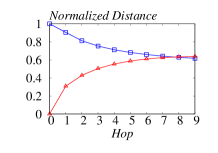
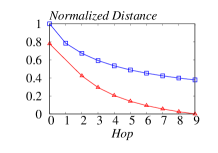
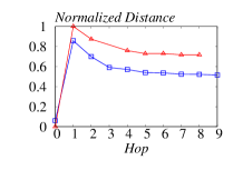
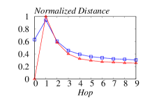
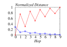
| (a) T-Finance | (b) YelpChi | (c) Questions |
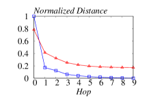
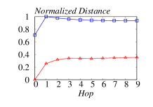
However, previous studies have overlooked the underlying properties associated with the smoothing process, which can serve as effective indicators for distinguishing anomalous nodes from normal nodes. In our investigation, we conduct a comprehensive analysis of the distances between node representations at each propagation hop and the converged representations obtained after an infinite number of hops. We calculate the average normalized distances for both anomalous and normal nodes. Notably, these distances exhibit distinct patterns across different types of nodes in real-world datasets, such as T-Finance, YelpChi, and Questions, as shown in Figure 1. Similar observations on other datasets can be found in Appendix A.7. To gain a deeper understanding of the underlying reasons for this phenomenon, we conduct theoretical analysis, revealing that the smoothing patterns are closely related to anomalous properties of nodes, originating from the spectral space of the graph. Moreover, given the strong relationship between the smoothing issues and the spectral space, we further explore the spectral energy of the graph (Dong et al., 2024; Tang et al., 2022). Our findings show that the Dirichlet Energy (Zhou et al., 2021), which represents the smoothness of a graph, plays a similar role as the spectral energy, which can be utilized as coefficients of node representations.
Motivated by the experimental and theoretical results, we introduce SmoothGNN, a novel graph learning framework for unsupervised NAD tasks. To be specific, SmoothGNN consists of four components: the Smoothing Learning Component (SLC), the Smoothing-aware Spectral GNN (SSGNN), the Smoothing-aware Coefficients (SC), and the Smoothing-aware Measure (SMeasure) for NAD. The SLC serves as a feature augmentation module, explicitly capturing the different patterns of anomalous and normal nodes (observation in Figure 1). SSGNN is designed to learn node representations from the spectral space of the graph while effectively capturing distinct smoothing patterns. Furthermore, we provide a theoretical analysis on the Dirichlet Energy, which can extract both smoothness and spectral energy information. Based on this analysis, we design the SC accordingly. During the training phase, we propose a loss function that incorporates both feature reconstruction and the SMeasure to optimize the model. Finally, we utilize the SMeasure as the anomaly score for each node during the inference phase. In contrast to previous work that primarily evaluated on small or synthetic datasets, we conduct experiments on large-scale real datasets commonly encountered in practical applications. In summary, the main contributions of our work are as follows:
-
•
To the best of our knowledge, we are the first to reveal that the smoothing issues can benefit NAD tasks, from both experimental and theoretical perspectives. Building on this insight, we introduce a novel SMeasure as the unsupervised anomaly measurement.
-
•
We propose SmoothGNN, a novel framework that captures information from both the smoothing process and spectral space of graphs, which can serve as a powerful backbone for NAD tasks.
-
•
We are the only work that conducts experiments on large real-world datasets for unsupervised NAD. Extensive experiments demonstrate the effectiveness and efficiency of our framework. Compared to state-of-the-art models, SmoothGNN achieves superior performance in terms of AUC and Precision metrics, with at least one order of magnitude speed-up.
2 Related Work
In recent years, unsupervised NAD has gained increasing interest within the graph learning community. Researchers have proposed a variety of models that can be broadly categorized into four groups: shallow models, reconstruction models, self-supervised models, and other models. Next, we briefly introduce several representative frameworks from these categories.
Shallow Models. Prior to the emergence of deep learning models, previous work mainly focuses on shallow models for the NAD task. For instance, Radar (Li et al., 2017) utilizes the residuals of attribute information and their coherence with network information to identify anomalous nodes. ANOMALOUS (Peng et al., 2018) introduces a joint framework for NAD based on residual analysis. These models primarily leverage matrix decomposition and residual analysis, which inherently have limited capabilities in capturing the complex information underlying graph data.
Reconstruction Models. Reconstruction models are prevalent approaches in the field of unsupervised NAD, as the reconstruction errors of graph structures and node features inherently reflect the likelihood of a node being anomalous. Motivated by this, a prior work CLAD (Kim et al., 2023), proposes a label-aware reconstruction approach that utilizes Jensen-Shannon Divergence and Euclidean Distance. Besides, graph auto-encoders (GAEs) are widely adopted as reconstruction techniques. For example, GADNR (Roy et al., 2024) incorporates GAEs to reconstruct the neighborhood of nodes. Although previous studies have shown the effectiveness of graph reconstruction, it is worth noting that reconstructing graph structures can be computationally expensive. Moreover, experimental findings from GADbench (Tang et al., 2023) indicate that node feature reconstruction yields the most significant benefits for NAD. Therefore, a preferable choice is to focus exclusively on feature reconstruction, as introduced in the SmoothGNN framework.
Self-supervised Models. Aside from the reconstruction models, self-supervised models, particularly contrastive learning frameworks, are also popular choices in unsupervised NAD. For instance, NLGAD (Duan et al., 2023c) constructs multi-scale contrastive learning networks to estimate the normality for nodes. Similarly, GRADATE (Duan et al., 2023a) presents a multi-scale contrastive learning framework with subgraph-subgraph contrast to capture the local properties of nodes. Other examples include PREM (Pan et al., 2023) and ARISE (Duan et al., 2023b), which employ node-subgraph contrast and node-node contrast to learn node representations, reflecting both local and global views of the graph. A recent study, TAM (Qiao & Pang, 2023), leverages data augmentation to generate multi-view graphs, enabling the examination of the consistency of the local feature information within node neighborhoods. Based on the observation of local node affinity, TAM introduces a local affinity score to measure the probability of a node being anomalous, highlighting the importance of designing new measures for NAD. In contrast, SmoothGNN introduces the SMeasure to detect anomalous nodes, which utilizes a more flexible way to capture the anomalous properties of the nodes. Moreover, the SMeasure requires fewer computational resources, enabling SmoothGNN to be applied to large-scale datasets.
Other Models. In addition to the above-mentioned models, there are other notable models such as RAND (Bei et al., 2023) and VGOD (Huang et al., 2023). RAND is the first work, to the best of our knowledge, that leverages reinforcement learning in the unsupervised NAD task. It introduces an anomaly-aware aggregator to amplify messages from reliable neighbors. On the other hand, VGOD presents a mixed-type framework that combines graph reconstruction and self-supervised models. It incorporates a variance-based module to sample positive and negative pairs for contrastive learning, along with an attribute reconstruction module to reconstruct node features. In contrast to these works, our SmoothGNN framework adopts a different strategy by utilizing feature reconstruction to assist in learning the SMeasure score, which serves as part of the objective function. This approach achieves superior performance while requiring significantly less running time.
3 Method: SmoothGNN
Our observation in Section 1 highlights the different smoothing patterns exhibited by anomalous and normal nodes. In Section 3.1, we first present the background knowledge for the following analysis. Subsequently, Section 3.2 provides a comprehensive theoretical analysis of smoothing patterns. This analysis serves as the motivation behind the design of two key components, SLC and SSGNN in SmoothGNN framework, to be elaborated in Sections 3.3 and 3.4, respectively. Moreover, our theoretical analysis in Section 3.2 reveals that the spectral energy of the graph can be represented by the Dirichlet Energy, which inspires us to employ the Dirichlet Energy as effective coefficients for node representations, to be detailed in Section 3.5. Finally, Section 3.6 elaborates on the overall objective function, including a feature reconstruction loss and the proposed novel Smeasure.
3.1 Preliminaries
Notation. Let denote a connected undirected graph with nodes and edges, where is node features and is the adjacency matrix. Let if there exists an edge between node and , otherwise . denotes the degree matrix. The adjacency matrix and degree matrix of graph with self-loop can be defined as and , respectively, where is an identity matrix. The Laplacian matrix is then defined as . It can also be decomposed by , where represents orthonormal eigenvectors and the corresponding eigenvalues are sorted in ascending order, i.e. . Let be a signal on graph , the graph convolution operation between a signal and a graph filter is then defined as , where the parameter is spectral filter coefficient vector.
Spectral GNN. Graph convolution operations (Defferrard et al., 2016; Kipf & Welling, 2017) can be approximated by the -th order polynomial of Laplacians:
where corresponds to polynomial coefficients. In the following Section 3.2, the prevalent graph convolution operation is demonstrated to have a strong relation with graph smoothing patterns. This key insight motivates the design of SmoothGNN, which can capture information from graph spectral space and anomalous properties behind smoothing patterns.
Dirichlet Energy. Smoothing issues can be a challenging problem for GNNs. It is shown to be closely related to the Dirichlet energy of the graph (Zhang et al., 2021), which can be defined as
where represents the -th entry of the adjacency matrix , and is the degree of node . Dirichlet Energy serves as a measure of the smoothness of node features within neighborhoods. Given its intrinsic connection to the smoothing patterns of nodes, we delve deeper into this relationship in Section 3.2. Our analysis reveals that the Dirichlet Energy exhibits a strong correlation with the spectral space and can be used as the coefficients for node representations.
3.2 Theoretical Analysis: Connection among Smoothing Patterns, Spectral Space, and NAD
As discussed in Section 1, Smoothing issues have been extensively studied in the graph learning area. However, previous studies primarily focus on highlighting its negative aspects. This motivates us to explore the potential positive implications of smoothing issues. To this end, we conduct a detailed analysis to demonstrate how smoothing patterns can reveal anomalous properties of nodes as shown below. All the proofs of our theorems can be found in Appendix A.1.
Based on previous research (Qiao & Pang, 2023; Gao et al., 2023), both local views, such as neighboring nodes and features, and global views, which encompass statistical information of entire graphs, contribute to the detection of node anomalies. The following theorem indicates that smoothing patterns can be represented by an augmented propagation matrix, which is aware of both local and global information. Thus, the smoothing patterns can be an effective identifier for NAD tasks.
Theorem 1.
Let denote the propagation matrix given the adjacency matrix . For an augmented propagation matrix , where represents the converged status of , we can derive with -th entry , where is the indicator function, is the -th entry of the adjacency matrix, is the degree of node , and , represent the number of edges and nodes, respectively.
Theorem 1 shows that, when the graph signal propagates on the augmented propagation matrix , the resulting node presentation becomes aware of local structures and individual node features. In addition, since this augmented propagation matrix not only propagates graph signal through edge connection but also assigns the signal a transformation of statistical information of graph as coefficients, serving as the attention mechanism, it highlights the disparities arising from global views. Thus, the augmented propagation offers a more precise indication of the underlying properties of anomalous and normal nodes compared to the original propagation. This observation is also supported by the empirical evidence of different smoothing patterns shown in Section 1. Leveraging the comprehensive information contained by the augmented matrix, we employ it in the design of the SLC in Section 3.3 and the SMeasure in Section 3.6.
Moreover, previous studies (Tang et al., 2022; Dong et al., 2024) have demonstrated a strong connection between graph anomalies and graph spectral space. Building upon Theorem 1, which establishes the close relationship of the augmented propagation matrix with graph anomalies, we investigate the connection between the augmented propagation matrix and the graph spectral space. The following theorem demonstrates that the column vectors of the augmented propagation matrix can be represented by a polynomial combination of graph convolution operations, further indicating the strong correlation between the augmented propagation matrix and the graph spectral space.
Theorem 2.
The augmented propagation matrix after hops of propagation can be expressed by , where is a column vector of , is the spectral filter coefficients, and represent the linear combinations of the eigenvectors of and , respectively.
Theorem 2 illustrates that the augmented propagation matrix can be represented by the spectral filter (introduced in Section 3.1). This motivates us to design SSGNN, a spectral GNN that not only leverages information from the spectral space but also captures smoothing patterns, to be elaborated in Section 3.4. Besides, RQGNN (Dong et al., 2024) has shown that the coefficients of node representations can be guided by spectral energy. Given our findings that reveal the strong connection between smoothing patterns and spectral space, we aim to explore new coefficients that can effectively capture both smoothing patterns and spectral energy. Firstly, we provide the definition of spectral energy following previous studies (Tang et al., 2022; Dong et al., 2024).
Definition 1 ((Tang et al., 2022; Dong et al., 2024)).
Given the graph Laplacian matrix and a graph signal , the graph Fouier Transformation of is defined as . The spectral energy of the graph at can be expressed as .
Based on Definition 1, we have the following theorem, which shows that Dirichlet Energy can serve a similar role as spectral energy.
Theorem 3.
Given a graph with Laplacian matrix and a graph signal , the Dirichlet Energy can be represented by , where the is the -th eigenvalue of .
Recap from Section 3.1 that Dirichlet Energy characterizes the smoothness of node representations within their neighborhoods, which is complementary to the previous individual view depicted in Figure 1. Theorem 3 shows that the smoothing patterns of nodes can also be effectively represented using a polynomial combination of the spectral energy. Building on this finding, we introduce Smoothness-aware Coefficients (SC) as the coefficients of node representations, which will be discussed in Section 3.5.
Based on the aforementioned theorems, we propose different components of our SmoothGNN. To achieve a balance between effectiveness and efficiency, we further analyze the maximum propagation hops of SmoothGNN that do not provide additional information. Specifically, if the node representations have already reached a converged state, additional layers of SmoothGNN will not provide substantial benefits but will consume additional computational sources. Therefore, we determine the layers of SmoothGNN based on Theorem 4. To achieve this, we first define -smoothing (Rong et al., 2020) and then illustrate the theorem of the converged hop.
Definition 2 ((Rong et al., 2020)).
For any GNN, we call it suffers from -smoothing if and only if after hops of propagation, the resulting feature matrix at hop has a distance no larger than with respect to a subspace , namely, , where represents the Frobenius norm from to the subspace .
Theorem 4.
Given the subspace with threshold , a GNN model will suffer from -smoothing issue when the propagation hop , where is the largest singular value of the graph filters over all layers, is the second largest eigenvalue of the propagation matrix, and is the feature matrix of graph .
Theorem 4 provides a theoretical guarantee regarding the maximum propagation hops that can contribute to the learning process. In Section 4 and Appendix A.5, we further observe that the required propagation hop is directly proportional to the number of nodes in the graph. In the following sections, we elaborate on our SmoothGNN framework in detail.
3.3 Smoothing Learning Component
Motivated by Theorem 1 and the observation in Section 1, we propose a simple yet powerful component to capture the smoothing patterns of nodes. Specifically, we first calculate the augmented propagation matrix for . Next, we employ a set of MLPs to obtain the latent node representations propagated on each . Finally, an additional MLP is adopted to fuse the node representations obtained from different propagation hops. Let denote the node features after the -th feature transformation, the representation of the -th node in SLC can be expressed as:
| (1) |
In addition to explicitly learning from smoothing patterns, it is crucial for the model to implicitly capture information from the graph topology and node features. The combination of explicit and implicit learning enables the collection of comprehensive information required for NAD tasks. The details of implicit learning are presented as follows.
3.4 Smoothing-aware Spectral GNN
As stated in Theorem 2, the augmented propagation matrix after hops of propagation can be represented as , demonstrating the capability of the graph spectral space to reveal underlying node properties for NAD. This motivates our design of a spectral GNN to learn node representations. Considering augmented propagation matrices, it is essential to design a spectral GNN that captures information from all hops of propagation. Therefore, employing a polynomial combination of graph spectral filters as the graph convolution operation filter can be a natural choice. To maintain the simplicity of our framework, we leverage -th order polynomial of graph Laplacian as the backbone filter. Specifically, let denote the graph convolution operation, we have:
| (2) |
Similar to SLC, we consider as node features after -th feature transformation for each graph convolution operation. Subsequently, we employ an MLP to fuse the spectral node representations obtained from each propagation hop to generate the final node representations. The representation of the -th node can be expressed as follows:
| (3) |
Note that we utilize shared weights in SLC and SSGNN. By incorporating these two components, our framework can capture information from both spectral space and smoothing patterns. In addition, as discussed in 3.2, the coefficients of the final representations guided by spectral energy enable the framework to effectively represent different dimensions of spectral space. To achieve this, we further introduce SC in Section 3.5.
3.5 Smoothing-aware Coefficients
Theorem 3 shows that the Dirichlet Energy can be interpreted as a polynomial combination of spectral energy. Motivated by (Dong et al., 2024), we design SC for node representations. Specifically, we first calculate the Dirichlet Energy for the graph, which can be expressed as:
| (4) |
where denotes the diagonal entries of a square matrix. Subsequently, we apply the Sigmoid function to rescale the coefficients, i.e., . Finally, we utilize element-wise multiplication to rearrange the coefficients of representations and for .
| (5) |
The final representations generated by SLC and SSGNN in SmoothGNN is utilized to calculate the loss function and the SMeasure.
3.6 Smoothing-aware Measure
According to previous work (Huang et al., 2023), feature reconstruction loss can assist in learning effective measures for NAD. This inspires us to design a loss function combined with two components: the feature reconstruction loss and the SMeasure. For the feature reconstruction loss, we use to reconstruct the original feature.
| (6) |
where is the -th row of the original feature matrix . For the SMeasure, we leverage the representations obtained from SLC as it naturally captures the underlying differences in the smoothing patterns. To be specific, we define the SMeasure as follows:
| (7) |
where represents the Sigmoid function, and represents the column-wise average function, which aims to aggregate the smoothing patterns across all dimensions. Based on the SMeasure, we further define the smoothing-based loss function:
| (8) |
The final loss function is a combination of both and :
| (9) |
The loss function is carefully designed to leverage the feature reconstruction loss to facilitate the learning process of the SMeasure. This combination enables the loss function to capture valuable information from the smoothing patterns and the reconstruction errors across different nodes. Minimizing this loss function empowers the model to effectively reduce the presence of anomalous nodes in the predicted results, thereby addressing the challenge of extremely unbalanced data in NAD. With this comprehensive loss function, our SmoothGNN can optimize the shared weights of two key components. Consequently, our framework excels in learning more accurate node representations for the task of detecting anomalous nodes.
4 Experiments
4.1 Experimental Setup
| Categories | Datasets | #Nodes | #Edges | #Feature | Avg. Degree | Anomaly Ratio |
|---|---|---|---|---|---|---|
| Small | 10,984 | 168,016 | 64 | 15.30 | 3.33% | |
| Tolokers | 11,758 | 519,000 | 10 | 44.14 | 21.82% | |
| Amazon | 11,944 | 4,398,392 | 25 | 368.25 | 6.87% | |
| Medium | T-Finance | 39,357 | 21,222,543 | 10 | 539.23 | 4.58% |
| YelpChi | 45,954 | 3,846,979 | 32 | 83.71 | 14.53% | |
| Questions | 48,921 | 153,540 | 301 | 3.14 | 2.98% | |
| Large | Elliptic | 203,769 | 234,355 | 167 | 1.15 | 9.76% |
| DGraph-Fin | 3,700,550 | 4,300,999 | 17 | 1.16 | 1.27% | |
| T-Social | 5,781,065 | 73,105,508 | 10 | 12.65 | 3.01% |
Datasets. We evaluate SmoothGNN on 9 real-world datasets, including Reddit, Tolokers, Amazon, T-Finance, YelpChi, Questions, Elliptic, DGraph-Fin, and T-Social. These datasets are obtained from the benchmark paper (Tang et al., 2023), consisting of various types of networks and corresponding anomalous nodes. Based on their number of nodes, we divide these datasets into three categories, Small, Medium, and Large, as shown in Table 1. Note that unlike previous work in the unsupervised NAD area, we only utilize real-world datasets with a sufficient number of nodes. Furthermore, to the best of our knowledge, SmoothGNN is the only model in this field that conducts experiments on large-scale datasets like T-Social to validate the efficiency and effectiveness of the model.
Baselines. We compare RQGNN against 11 SOTA competitors, including shallow models, reconstruction models, self-supervised models, and other models.
- •
- •
- •
- •
Experimental Settings. In line with the experimental settings of prior research (Liu et al., 2022; Huang et al., 2023; Qiao & Pang, 2023), we conduct transductive experiments on these datasets. The parameters of SmoothGNN are set according to the categories of the datasets. The specific parameters for each category can be found in Appendix A.3. To ensure a fair comparison, we obtain the source code of all competitors from GitHub and execute these models using the default parameter settings suggested by their authors.
4.2 Main Results
| Shallow | Reconstruction | Self-supervised | Other | ||||||||||
|---|---|---|---|---|---|---|---|---|---|---|---|---|---|
| Datasets | Metrics | RADAR | ANOMALOUS | CLAD | GADNR | NLGAD | GRADATE | PREM | ARISE | TAM | RAND | VGOD | SmoothGNN |
| AUC | 0.4372 | 0.4481 | 0.5784 | 0.5532 | 0.5380 | 0.5261 | 0.5518 | 0.5273 | 0.5729 | 0.5417 | 0.4931 | 0.5946 | |
| Precision | 0.0273 | 0.0309 | 0.0502 | 0.0373 | 0.0415 | 0.0393 | 0.0413 | 0.0402 | 0.0425 | 0.0356 | 0.0324 | 0.0438 | |
| Tolokers | AUC | 0.3625 | 0.3706 | 0.4061 | 0.5768 | 0.4825 | 0.5373 | 0.5654 | 0.5514 | 0.4699 | 0.4377 | 0.4988 | 0.6870 |
| Precision | 0.1713 | 0.1731 | 0.1921 | 0.2991 | 0.2025 | 0.2364 | 0.2590 | 0.2505 | 0.1963 | 0.1939 | 0.2212 | 0.3517 | |
| Amazon | AUC | 0.2318 | 0.2318 | 0.2026 | 0.2608 | 0.5425 | 0.4781 | 0.2782 | 0.4782 | 0.8028 | 0.3585 | 0.5182 | 0.8408 |
| Precision | 0.0439 | 0.0439 | 0.0401 | 0.0424 | 0.0991 | 0.0634 | 0.0744 | 0.0677 | 0.3322 | 0.0492 | 0.0779 | 0.3953 | |
| T-Finance | AUC | 0.2824 | 0.2824 | 0.1385 | 0.5798 | 0.5231 | 0.4063 | 0.4484 | 0.4667 | 0.6901 | 0.4380 | 0.4814 | 0.7556 |
| Precision | 0.0295 | 0.0295 | 0.0247 | 0.0542 | 0.0726 | 0.0376 | 0.0391 | 0.0393 | 0.1284 | 0.0403 | 0.0454 | 0.1408 | |
| YelpChi | AUC | 0.5261 | 0.5272 | 0.4755 | 0.4704 | 0.4981 | 0.4920 | 0.4900 | 0.4834 | 0.5487 | 0.5052 | 0.4878 | 0.5758 |
| Precision | 0.1822 | 0.1700 | 0.1284 | 0.1395 | 0.1469 | 0.1447 | 0.1378 | 0.1415 | 0.1733 | 0.1470 | 0.1345 | 0.1823 | |
| Questions | AUC | 0.4963 | 0.4965 | 0.6207 | 0.5875 | 0.5428 | 0.5539 | 0.6033 | 0.6241 | 0.5042 | 0.6164 | 0.5075 | 0.6444 |
| Precision | 0.0279 | 0.0279 | 0.0512 | 0.0577 | 0.0348 | 0.0350 | 0.0430 | 0.0619 | 0.0395 | 0.0442 | 0.0299 | 0.0592 | |
| Elliptic | AUC | - | - | 0.4192 | 0.4001 | 0.4977 | - | 0.4978 | - | - | - | 0.5723 | 0.5729 |
| Precision | - | - | 0.0807 | 0.0778 | 0.1009 | - | 0.0905 | - | - | - | 0.1256 | 0.1161 | |
| DGraph-Fin | AUC | - | - | - | - | - | - | - | - | - | - | 0.5456 | 0.6499 |
| Precision | - | - | - | - | - | - | - | - | - | - | 0.0148 | 0.0199 | |
| T-social | AUC | - | - | - | - | - | - | - | - | - | - | 0.5999 | 0.7034 |
| Precision | - | - | - | - | - | - | - | - | - | - | 0.0351 | 0.0631 | |
| Shallow | Reconstruction | Self-Supervised | Other | |||||||||
|---|---|---|---|---|---|---|---|---|---|---|---|---|
| Datasets | RADAR | ANOMALOUS | CLAD | GADNR | NLGAD | GRADATE | PREM | ARISE | TAM | RAND | VGOD | SmoothGNN |
| 55.57 | 42.25 | 11.14 | 692.66 | 10886.19 | 7562.59 | 73.52 | 1261.99 | 5050.89 | 310.11 | 39.86 | 7.02 | |
| Tolokers | 57.51 | 40.94 | 52.91 | 861.95 | 10504.91 | 7824.63 | 74.80 | 1281.71 | 5668.91 | 367.03 | 177.42 | 6.99 |
| Amazon | 42.79 | 38.07 | 431.20 | 2048.72 | 10649.83 | 7856.41 | 130.57 | 1267.38 | 1148.24 | 593.75 | 1517.70 | 7.19 |
| T-Finance | 500.19 | 360.97 | 2161.16 | 14255.00 | 35648.72 | 30341.65 | 266.33 | 4223.50 | 81238.60 | 6746.10 | 5998.08 | 16.69 |
| YelpChi | 730.81 | 513.83 | 418.95 | 5046.51 | 42435.07 | 35938.21 | 308.68 | 5042.99 | 102232.07 | 6588.60 | 1283.10 | 19.37 |
| Questions | 1205.05 | 1114.22 | 52.65 | 2795.99 | 51270.03 | 44235.87 | 409.45 | 6135.88 | 11603.81 | 7364.07 | 86.12 | 32.68 |
| Elliptic | - | - | 421.17 | 12568.50 | 193304.73 | - | 2149.77 | - | - | - | 231.63 | 205.10 |
| DGraph-Fin | - | - | - | - | - | - | - | - | - | - | 3420.84 | 2924.99 |
| T-Social | - | - | - | - | - | - | - | - | - | - | 22984.10 | 4877.05 |
The performance of SmoothGNN is evaluated against different SOTA models in the NAD field. Table 2 reports the AUC and Precision scores of each model across 9 datasets. The best result on each dataset is highlighted in boldface. Our key observations are as follows.
Firstly, most existing unsupervised NAD models struggle to handle large datasets, with only VGOD and the proposed SmoothGNN successfully running on the two largest datasets. This highlights the need for the development of unsupervised models capable of handling large-scale datasets.
Shallow models like Radar and ANOMALOUS apply residual analysis to solve NAD, which poses challenges in capturing the underlying anomalous properties from a spectral perspective. In comparison, SmoothGNN takes the lead by 29.37% and 29.03% in terms of AUC, and 11.52% and 11.63% in terms of Precision on average across 6 datasets, respectively. Moreover, these shallow models are unable to handle the 3 large datasets due to memory constraints. These results demonstrate that shallow models are both time-consuming and ineffective when applied to real-world NAD datasets.
Next, we examine reconstruction approaches CLAD and GADNR, which utilize reconstruction techniques to detect graph anomalies. While these models leverage both structure and feature reconstruction to calculate the anomaly score for each node, they fail to capture the information from the spectral domain, leading to inferior performance. SmoothGNN outperforms these models by 26.14% and 17.75% in terms of AUC, and 10.31% and 8.30% in terms of Precision on average across different datasets, respectively.
We then compare SmoothGNN with self-supervised models NLGAD, GRADATE, PREM, ARISE, and TAM. Although self-supervised learning approaches can boost the performance of unsupervised frameworks, their high memory requirements and computational costs make them prohibitive for large datasets. While NLGAD and PREM utilize sparse techniques to address these issues, they still cannot run on the two largest datasets. In comparison, SmoothGNN achieves an improvement of 14.95% and 17.66% in terms of AUC, and 8.44% and 8.63% in terms of Precision on average across 7 datasets, respectively. Besides, SmoothGNN also outperforms other models like GRADATE and ARISE by 18.41% and 16.12% in terms of AUC, and 10.28% and 9.53% in terms of Precision on average across 7 datasets, respectively. In addition, TAM is the best rival in terms of performance, but its high memory usage and running time make it unable to run on large datasets. Across 6 datasets, SmoothGNN surpasses TAM by 8.49% in terms of AUC and 4.35% in terms of Precision on average.
Finally, we examine the results of other approaches RAND and VGOD. RAND represents a novel direction for unsupervised NAD tasks but fails to leverage more advanced graph properties, like smoothing patterns, to guide the learning process. As a result, SmoothGNN outperforms RAND by 20.01% in terms of AUC, and 11.05% in terms of Precision on average across 6 datasets. On the other hand, VGOD is the only competitor capable of running on all the datasets, demonstrating the benefits of combining feature reconstruction and novel measures. However, SmoothGNN leverages similar techniques more efficiently and effectively, surpassing VGOD by 14.66% in terms of AUC and 7.28% in terms of Precision on average across all datasets, with a 75x speed-up in running time.
4.3 Alternative Smoothing Patterns
| Datasets | Tolokers | Amazon | T-Finance | YelpChi | Questions | Elliptic | DGraph-Fin | |||||||||
|---|---|---|---|---|---|---|---|---|---|---|---|---|---|---|---|---|
| Metrics | AUC | Precision | AUC | Precision | AUC | Precision | AUC | Precision | AUC | Precision | AUC | Precision | AUC | Precision | AUC | Precision |
| SmoothGNN | 0.5946 | 0.0438 | 0.6870 | 0.3517 | 0.8408 | 0.3953 | 0.7556 | 0.1408 | 0.5758 | 0.1823 | 0.6444 | 0.0592 | 0.5729 | 0.1161 | 0.6499 | 0.0199 |
| SmoothGNN-A | 0.5919 | 0.0486 | 0.6731 | 0.3340 | 0.8008 | 0.2719 | 0.7408 | 0.1099 | 0.5697 | 0.1887 | 0.6388 | 0.0527 | 0.5695 | 0.1136 | 0.5893 | 0.0164 |
In addition to the smoothing patterns observed in vanilla GNN, graph learning models like APPNP (Klicpera et al., 2019) also converge to a steady state. Specifically, the converged state of APPNP can be expressed as
where is the teleport probability. To investigate whether any smoothing pattern can be utilized for detecting anomalous nodes, we modify the graph convolution operation in SSGNN with APPNP update rule , and replace with . The results of this modified model, denoted as SmoothGNN-A, are shown in Table 4. We observe that by employing alternative smoothing patterns, the framework can still effectively detect anomalous nodes, thus validating that smoothing patterns serve as accurate identifiers for NAD tasks. However, based on the comparison between SmoothGNN and SmoothGNN-A in Table 4, we find SmoothGNN can achieve relatively better performance in most datasets. These results demonstrate information from spectral space can also be important in NAD tasks.
5 Conclusion
In this paper, we introduce the smoothing patterns into the NAD task. We identify differences in the smoothing patterns between anomalous and normal nodes, and further demonstrate the observation through comprehensive experiments and theoretical analysis. The combination of four components in SmoothGNN enables the model to capture information from both the spectral space and smoothing patterns, providing comprehensive perspectives for NAD tasks. Extensive experiments demonstrate that SmoothGNN consistently outperforms other SOTA competitors by a significant margin in terms of performance and running time, thus highlighting the effectiveness and efficiency of leveraging smoothing patterns in the NAD area.
References
- Akoglu et al. (2015) Leman Akoglu, Hanghang Tong, and Danai Koutra. Graph based anomaly detection and description: a survey. Data Min. Knowl. Discov., pp. 626–688, 2015.
- Bei et al. (2023) Yuanchen Bei, Sheng Zhou, Qiaoyu Tan, Hao Xu, Hao Chen, Zhao Li, and Jiajun Bu. Reinforcement neighborhood selection for unsupervised graph anomaly detection. In ICDM, pp. 11–20, 2023.
- Chen et al. (2020) Ming Chen, Zhewei Wei, Zengfeng Huang, Bolin Ding, and Yaliang Li. Simple and deep graph convolutional networks. In ICML, pp. 1725–1735, 2020.
- Chung (1997) F. R. K. Chung. Spectral Graph Theory. American Mathematical Society, 1997.
- Defferrard et al. (2016) Michaël Defferrard, Xavier Bresson, and Pierre Vandergheynst. Convolutional neural networks on graphs with fast localized spectral filtering. In NeurIPS, pp. 3837–3845, 2016.
- Dong et al. (2024) Xiangyu Dong, Xingyi Zhang, and Sibo Wang. Rayleigh quotient graph neural networks for graph-level anomaly detection. In ICLR, pp. 1–19, 2024.
- Dou et al. (2020) Yingtong Dou, Zhiwei Liu, Li Sun, Yutong Deng, Hao Peng, and Philip S. Yu. Enhancing graph neural network-based fraud detectors against camouflaged fraudsters. In CIKM, pp. 315–324, 2020.
- Duan et al. (2023a) Jingcan Duan, Siwei Wang, Pei Zhang, En Zhu, Jingtao Hu, Hu Jin, Yue Liu, and Zhibin Dong. Graph anomaly detection via multi-scale contrastive learning networks with augmented view. In AAAI, pp. 7459–7467, 2023a.
- Duan et al. (2023b) Jingcan Duan, Bin Xiao, Siwei Wang, Haifang Zhou , and Xinwang Liu. Arise: Graph anomaly detection on attributed networks via substructure awareness. IEEE Trans. Neural Networks Learn. Syst., pp. 1–14, 2023b.
- Duan et al. (2023c) Jingcan Duan, Pei Zhang, Siwei Wang, Jingtao Hu, Hu Jin, Jiaxin Zhang, Haifang Zhou, and Xinwang Liu. Normality learning-based graph anomaly detection via multi-scale contrastive learning. In ACM Multimedia, pp. 7502–7511, 2023c.
- Gao et al. (2023) Yuan Gao, Xiang Wang, Xiangnan He, Zhenguang Liu, Huamin Feng, and Yongdong Zhang. Addressing heterophily in graph anomaly detection: A perspective of graph spectrum. In WWW, pp. 1528–1538, 2023.
- Huang et al. (2022) Xuanwen Huang, Yang Yang, Yang Wang, Chunping Wang, Zhisheng Zhang, Jiarong Xu, Lei Chen, and Michalis Vazirgiannis. Dgraph: A large-scale financial dataset for graph anomaly detection. In NeurIPS, pp. 22765–22777, 2022.
- Huang et al. (2023) Yihong Huang, Liping Wang, Fan Zhang, and Xuemin Lin. Unsupervised graph outlier detection: Problem revisit, new insight, and superior method. In ICDE, pp. 2565–2578, 2023.
- Kim et al. (2023) Junghoon Kim, Yeonjun In, Kanghoon Yoon, Junmo Lee, and Chanyoung Park. Class label-aware graph anomaly detection. In CIKM, pp. 4008–4012, 2023.
- Kipf & Welling (2017) Thomas N. Kipf and Max Welling. Semi-supervised classification with graph convolutional networks. In ICLR, pp. 1–14, 2017.
- Klicpera et al. (2019) Johannes Klicpera, Aleksandar Bojchevski, and Stephan Günnemann. Predict then propagate: Graph neural networks meet personalized pagerank. In ICLR, pp. 1–15, 2019.
- Li et al. (2017) Jundong Li, Harsh Dani, Xia Hu, and Huan Liu. Radar: Residual analysis for anomaly detection in attributed networks. In IJCAI, pp. 2152–2158, 2017.
- Liu et al. (2022) Kay Liu, Yingtong Dou, Yue Zhao, Xueying Ding, Xiyang Hu, Ruitong Zhang, Kaize Ding, Canyu Chen, Hao Peng, Kai Shu, Lichao Sun, Jundong Li, George H. Chen, Zhihao Jia, and Philip S. Yu. BOND: benchmarking unsupervised outlier node detection on static attributed graphs. In NeurIPS, pp. 27021–27035, 2022.
- Liu et al. (2021) Yang Liu, Xiang Ao, Zidi Qin, Jianfeng Chi, Jinghua Feng, Hao Yang, and Qing He. Pick and choose: A gnn-based imbalanced learning approach for fraud detection. In WWW, pp. 3168–3177, 2021.
- Ma et al. (2023) Xiaoxiao Ma, Jia Wu, Shan Xue, Jian Yang, Chuan Zhou, Quan Z. Sheng, Hui Xiong, and Leman Akoglu. A comprehensive survey on graph anomaly detection with deep learning. IEEE Trans. Knowl. Data Eng., pp. 12012–12038, 2023.
- McAuley & Leskovec (2013) Julian J. McAuley and Jure Leskovec. From amateurs to connoisseurs: modeling the evolution of user expertise through online reviews. In WWW, pp. 897–908, 2013.
- Oono & Suzuki (2019) Kenta Oono and Taiji Suzuki. On asymptotic behaviors of graph cnns from dynamical systems perspective. ArXiv, 2019.
- Pan et al. (2023) Junjun Pan, Yixin Liu, Yizhen Zheng, and Shirui Pan. PREM: A simple yet effective approach for node-level graph anomaly detection. In ICDM, pp. 1253–1258, 2023.
- Peng et al. (2018) Zhen Peng, Minnan Luo, Jundong Li, Huan Liu, and Qinghua Zheng. ANOMALOUS: A joint modeling approach for anomaly detection on attributed networks. In IJCAI, pp. 3513–3519, 2018.
- Qiao & Pang (2023) Hezhe Qiao and Guansong Pang. Truncated affinity maximization: One-class homophily modeling for graph anomaly detection. In NeurIPS, pp. 49490–49512, 2023.
- Rong et al. (2020) Yu Rong, Wenbing Huang, Tingyang Xu, and Junzhou Huang. Dropedge: Towards deep graph convolutional networks on node classification. In ICLR, pp. 1–17, 2020.
- Roy et al. (2024) Amit Roy, Juan Shu, Jia Li, Carl Yang, Olivier Elshocht, Jeroen Smeets, and Pan Li. GAD-NR: graph anomaly detection via neighborhood reconstruction. In WSDM, pp. 576–585, 2024.
- Sun et al. (2022) Shuyuan Sun, Yiyang Jiang, Fan Yang, Bei Yu, and Xuan Zeng. Efficient hotspot detection via graph neural network. In DATE, pp. 1233–1238, 2022.
- Tang et al. (2022) Jianheng Tang, Jiajin Li, Ziqi Gao, and Jia Li. Rethinking graph neural networks for anomaly detection. In ICML, pp. 21076–21089, 2022.
- Tang et al. (2023) Jianheng Tang, Fengrui Hua, Ziqi Gao, Peilin Zhao, and Jia Li. Gadbench: Revisiting and benchmarking supervised graph anomaly detection. In NeurIPS, pp. 29628–29653, 2023.
- Zhang et al. (2021) Wentao Zhang, Mingyu Yang, Zeang Sheng, Yang Li, Wen Ouyang, Yangyu Tao, Zhi Yang, and Bin Cui. Node dependent local smoothing for scalable graph learning. In NeurIPS, pp. 20321–20332, 2021.
- Zhou et al. (2021) Kaixiong Zhou, Xiao Huang, Daochen Zha, Rui Chen, Li Li, Soo-Hyun Choi, and Xia Hu. Dirichlet energy constrained learning for deep graph neural networks. In NeurIPS, pp. 21834–21846, 2021.
Appendix A Appendix
A.1 Proofs
Proof of Theorem 1. The following lemma from previous work (Chen et al., 2020) is used for the proof.
Lemma 1.
Let denote the propagation matrix given the adjacency matrix , we have:
First, we need to derive . For , we have:
Then, we can derive that
Proof of Theorem 2. Based on the proof in Section "The stable distribution" in the book (Chung, 1997), for the column vector in augmented matrix we have:
where is the degree matrix of graph , is the -th eigenvalue of , is the -th eigenvector of , and is the coefficient related to . Then, let be the -th eigenvalue of and be the -th eigenvalue of , we have:
Then we replace in with , we have . By applying Tayler’s expansion to it, we have:
Finally, we can get
Proof of Theorem 3. For simplicity, let denote a normalized graph signal in the graph, we have:
Following the theorem in previous work (Dong et al., 2024), we have:
Proof of Theorem 4. The following corollary from previous work (Oono & Suzuki, 2019) is used for the proof.
Corollary 1.
Let be the eigenvalues of , sorted in ascending order. Suppose the multiplicity of the largest eigenvalue is , i.e.,. And the second largest eigenvalue can be defined as
Let be the eigenspace associated with , then we can assume that has an orthonormal basis that consists of non-negative vectors, and then we have:
where implying the output of the -th layer of GNN on exponentially approaches .
Based on the above corollary, we have:
When the GNN reaches -smoothing, we have:
And since , then we have , we have:
A.2 Algorithm
The detailed training process is shown in Algorithm 1. We use the trained model of the final epoch to conduct inference. The loss function is calculated using and , and the anomaly score is calculated for each node using as shown in Section 3.6.
A.3 Experimental Settings
| Categories | Learning Rate | Hop | Weight Initialization | Epsilon | Hidden Dimensions |
|---|---|---|---|---|---|
| Small | 1e-4 | 4 | 0.05 | 0 | 64 |
| Medium | 5e-4 | 5 | 0.01 | 4e-3 | 64 |
| Large | 5e-4 | 6 | 0.05 | 4e-3 | 64 |
The parameters are set based on the number of nodes in different graphs as shown in Table 5. As we can see, the hidden dimensions remain stable for all three categories. However, the learning rate and number of propagation hops increase as the number of nodes grows. Besides, we employ approximation techniques to calculate the converged status of propagation, i.e., we only retain the values larger than the square of epsilon in the final matrix. For small graphs, we do not require approximation whereas for medium and large graphs, we set the epsilon to 4e-3. Furthermore, the weight initialization strategy varies across graph categories because the optimal starting point in the optimization process tends to differ depending on the graph characteristics. As for the experimental environment, we conduct all the experiments on CPU for fair comparison.
A.4 Ablation Study
| Datasets | Tolokers | Amazon | T-Finance | YelpChi | Questions | Elliptic | DGraph-Fin | T-Social | ||||||||||
|---|---|---|---|---|---|---|---|---|---|---|---|---|---|---|---|---|---|---|
| Metrics | AUC | Precision | AUC | Precision | AUC | Precision | AUC | Precision | AUC | Precision | AUC | Precision | AUC | Precision | AUC | Precision | AUC | Precision |
| SmoothGNN | 0.5946 | 0.0438 | 0.6870 | 0.3517 | 0.8408 | 0.3953 | 0.7556 | 0.1408 | 0.5758 | 0.1823 | 0.6444 | 0.0592 | 0.5729 | 0.1161 | 0.6499 | 0.0199 | 0.7034 | 0.0631 |
| without SC | 0.5437 | 0.0356 | 0.6115 | 0.2967 | 0.5131 | 0.0645 | 0.2869 | 0.0292 | 0.5715 | 0.1770 | 0.6260 | 0.0630 | 0.5596 | 0.1076 | 0.5868 | 0.0161 | 0.6639 | 0.0622 |
The ablation study for SC is presented in Table 6. Notably, without SC to rearrange the weights of different dimensions in the spectral space, the performance drops significantly compared to the original SmoothGNN, which demonstrates the utilization of SC can boost the performances. It also underscores that capturing the smoothing patterns from different views will help the learning of the node representations for NAD tasks.
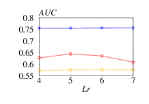
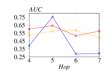
A.5 Parameter Analysis
|
|
|
| (a) Varying standard deviation | (b) Varying learning rate | (c) Varying hop |
 |
 |
| (a) Reddit | (b) Tolokers |
 |
 |
| (a) Amazon | (b) Elliptic |
 |
 |
| (a) DGraph-Fin | (b) T-Social |
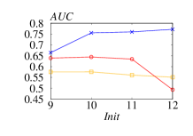
Next, we conduct experiments to analyze the effect of representative parameters: the standard deviation of weight initialization, the learning rate, and the number of propagation hops of SmoothGNN on T-Finance, YelpChi, and Questions datasets. Figure 2 reports the AUC of SmoothGNN as we vary the standard deviation from 9e-3 to 12e-3, the learning rate from 4e-4 to 7e-4, and the hop from 4 to 7. As we can observe, when we set the standard deviation to 10e-3, SmoothGNN achieves relatively satisfactory performances across these three datasets. In terms of learning rate, SmoothGNN exhibits relatively stable performance, but we can identify an optimal one, so we set the learning rate to 5e-5. Meanwhile, SmoothGNN shows a relatively stable and high performance in terms of all three presented datasets when we set the hop to 5. As a result, the hop is set to 5 in SmoothGNN.
A.6 Limitations
Although SmoothGNN achieves outstanding performance in all 9 real-world datasets compared to previous works, it still has some aspects to be improved. First, in this paper, we only discuss the smoothing patterns of GNN and APPNP, while there are other kinds of models in the field of graph learning. The performance of different types of smoothing patterns can vary due to their ability to capture additional information, such as spectral space. Second, Compared to semi-supervised and supervised NAD tasks, the performance of SmoothGNN is still unsatisfactory. Hence, it is also interesting to employ smoothing patterns in semi-supervised and supervised NAD tasks. Third, we only present the effectiveness of smoothing patterns in the NAD area, but applying smoothing patterns to other related fields can be meaningful as well.
A.7 Observations
Observations from the additional datasets presented in Figure 3, 4, and 5 further reinforce our findings. These figures clearly show that the smoothing patterns of anomalous and normal nodes exhibit distinct trends and scales. Our theoretical analysis and experimental results indicate that SmoothGNN is capable of detecting even subtle differences in these smoothing patterns. This sensitivity to nuanced smoothness characteristics is the key strength of the proposed approach.