Subspace Node Pruning

Abstract

A significant increase in the commercial use of deep neural network models increases the need for efficient AI. Node pruning is the art of removing computational units such as neurons, filters, attention heads, or even entire layers while keeping network performance at a maximum. This can significantly reduce the inference time of a deep network and thus enhance its efficiency. Few of the previous works have exploited the ability to recover performance by reorganizing network parameters while pruning. In this work, we propose to create a subspace from unit activations which enables node pruning while recovering maximum accuracy. We identify that for effective node pruning, a subspace can be created using a triangular transformation matrix, which we show to be equivalent to Gram-Schmidt orthogonalization, which automates this procedure. We further improve this method by reorganizing the network prior to subspace formation. Finally, we leverage the orthogonal subspaces to identify layer-wise pruning ratios appropriate to retain a significant amount of the layer-wise information. We show that this measure outperforms existing pruning methods on VGG networks. We further show that our method can be extended to other network architectures such as residual networks.

1 Introduction

After significant progress in the development of neural networks by the research community, commercial interest, especially in generative modelling, has taken off. Evermore capable models spark private and public interest, excitement, and engagement. However, the computational resources required to train and run these models are immense and neural networks have long exceeded the computational capacity of general purpose hardware. That is, they require large computer clusters and custom hardware/software solutions for training and inference.

To reduce the computational footprint of these models, a variety of approaches have been developed. These range from low-level hardware optimizations  (Choquette et al.,, 2021; Jouppi et al.,, 2018) to high-level software developments (Paszke et al.,, 2019; Abadi et al.,, 2015; Bradbury et al.,, 2018). Additionally, the representations of models in software have been made more compact with quantization methods (Krishnamoorthi,, 2018; Gholami et al.,, 2022).

Beyond optimization at the implementation level, powerful methods exist for reducing the size of models via different kinds of network compression. Compression of networks involves the reduction of the number of parameters and thereby (hopefully) the computational time required for computation. Network compression is possible due to the fact that deep neural networks are found to be significantly over-parameterized in practice, with sometimes orders of magnitude more parameters than should be necessary for computations (Frankle and Carbin,, 2018). Compression methods range from methods for network distillation, in which smaller networks are trained from scratch to reproduce the outputs of larger networks (Gou et al.,, 2021), to the systematic pruning of weights and nodes from trained networks. In this work, we focus on the sub-field of network pruning and develop a new state-of-the-art method within this domain.

Pruning neural networks

The goal of neural network pruning is to reduce the computational execution (inference) time of a model. Since the parameters of a model are dominated by the elements within the weight matrices, this means removing these parameters in some fashion. However, unstructured approaches to pruning of the weights of a model result in arbitrarily sparse matrices whose implementations cannot easily be accelerated at compute time. It is therefore desirable to prune whole nodes, convolutional filters, transformer heads, or other structured groups of parameters. Herein, we refer to any of these sub-parts of networks as network ‘elements’. Thus, the question is posed: how should one choose which elements of a network to prune first?

In theory, one might choose to remove units with least ‘importance’ from a network. Optimally, the units with least importance would be those whose absence has the least impact on network peformance. However, effectively and efficiently measuring the ‘importance scores’ of network elements is unclear. A number of heuristics have been developed with this goal in mind. First, and most simply, the magnitude of weights (Han et al.,, 2015) has been used as a proxy of their importance. Similarly, on a node/filter level the total summed magnitude (or summed squared magnitude) of incident weights to a convolutional filter has been used as an importance score for that filter (Li et al.,, 2016). These are by far the simplest methods for identifying node for pruning, which also do not require the passing of data through a model while measuring importance scores.

Methods of greater complexity are ‘data-driven’, making use of training data for forward (and in some cases backward) passes to measure importance scores. Molchanov et al., (2016, 2019) found that the square summed weight-gradient multiplication of weights incident to a node/filter can be used as a theoretically justified importance score under a linear approximation of a network via a 1-order Taylor-expansion (and similarly for the 2-order case). Chin et al., (2018) further improved upon this by introducing a layer-compensated pruning method that uses meta-learning to learn a set of latent variables that compensate for the layer-wise approximation error of the importance scores. Luo et al., (2017) went further by using a greedy (and computationally expensive) selection method to test all units/filters in a layer for those which, when pruned, have a minimal impact on the output of the layer, their importance measure being the difference between a layer’s output with vs without each individual unit. A number of methods also make use of correlation measures of feature maps or filter/node outputs within or between layers, with greater correlations equated to lower importance scores due to the redundancy of these representations (Zhang et al., 2022a, ; Ayinde et al.,, 2019; Cuadros et al.,, 2020).

Aside from methods applicable to pretrained networks, there are a number of approaches for embedding importance measures within an architecture, requiring network retraining. These methods involve multiplication of filter/node outputs by a trainable scalar which is regularized (He et al.,, 2017; Huang and Wang,, 2018; Liu et al.,, 2018; Bui et al.,, 2023; Ye et al.,, 2018; Parikh et al.,, 2014; Zhang et al., 2022b, ). These methods are numerous but differ in their approach to training of these scalars (often in an interleaved fashion with the training of model parameters) but ultimately such scalars are trained to be an importance score which can be used to select units for pruning. Such an approach can also be used in a structured fashion to prune from more than just nodes but also, e.g., from layers in a residual network (Wen et al.,, 2016; Alvarez and Salzmann,, 2016; Gao et al.,, 2019). We do not go into great detail for methods which require network retraining. Instead we focus on methods which start with trained networks and attempt to find importance scores for direct pruning of pre-trained networks.

In this work, we introduce a novel structured pruning method inspired by low-rank approximation. First, we use a data pass to measure simple cross-correlation statistics of units within every network layer. Second, we rank and factorize units based upon their cross-correlations measured in step one. This effectively means that when we prune individual units, we simultaneously also optimally read-out the, now missing, contribution from the pruned unit based upon the statistics of responses of all other remaining units. Thus, units can be pruned at every layer while also being approximated by their remaining neighbours.

This approach requires no hyperparameters and can improve existing alternative node pruning methods by making use of them for the ranking stage. We show that this method retains higher performance while significantly reducing the memory and runtime footprint of our models compared to existing node pruning work by application to VGG (Simonyan and Zisserman,, 2014) and ResNet-18/50/101 (He et al.,, 2016).

2 Methods

In this work we solely consider pruning of trained systems, such that we can assume that we begin with a functional and highly-performant model for each task. As a motivating example, consider a typical deep neural network (DNN) architecture, in which the outputs at each layer, $l\in[1,\ldots,L]$, are defined as $\mathbf{X}_{l}=f_{l}(\mathbf{Y}_{l})=f_{l}(\mathbf{W}_{l-1}\mathbf{X}_{l-1})$, where $\mathbf{X}_{l}\in\mathbb{R}^{n_{l}\times s}$ is a tensor of outputs for layer $l$ consisting of $n_{l}$ feature elements (nodes) for $s$ samples. These layer outputs are composed based upon a matrix multiplication of the previous layer outputs, from weights $\mathbf{W}_{l}\in\mathbb{R}^{n_{l+1}\times n_{l}}$, and by an element-wise transfer function $f_{l}(\cdot)$ which is usually the same for all layers. The input to the network is given by $\mathbf{X}_{0}$, which is our input dataset. We consider these fully-connected deep neural networks to introduce our approach. However, we shall also treat convolution, and residual layers in the results that follow.

2.1 Existing approaches

As mentioned in the Introduction, a key first step to pruning network elements is identification of their importance score $I$. Existing methods use various heuristics for the determination of such an importance score (Han et al.,, 2015; Li et al.,, 2016; Molchanov et al.,, 2019). These importance scoring methods allow a ranking of units within a layer. However, when units are pruned based upon this ranking, the output of the next layer is changed and this introduction of error is left unexplained. Luo et al., (2017) attempted to solve this problem by linearly re-approximating the input-output transformation of a layer after pruning. Though this approach is effective, it requires prior knowledge of how much pruning is to be carried out at each network layer and is inflexible to this choice, requiring repetition of multiple computational steps should a practitioner wish to adjust pruning ratios.

2.2 Subspace node pruning

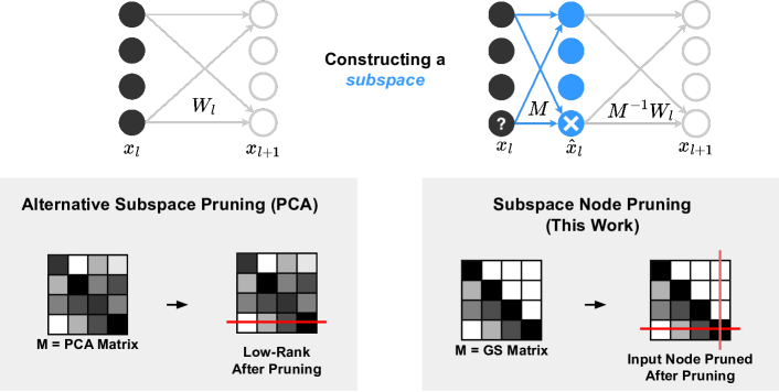
Figure 1: Subspace methods and node pruning. Top, we illustrate how our method involves the projection of unit activities at the input of a layer to a subspace. Bottom, We show how the projection matrix, $\mathbf{M}$, could be setup in a number of alternative ways (example given of PCA for comparison) but that we make use of an unnormalized Gram-Schmidt (GS) orthogonalization. Other subspace methods (like PCA) do not allow node pruning when the subpace is pruned, resulting in a low-rank approximation. However, in the case of a lower triangular projection matrix, pruning in the subspace is equivalent to node pruning.

In this work, we propose a novel approach in which node/filter activities are projected to a subspace from which pruning has a minimal impact on the network output. The subspace is constructed via a factorization process such that each unit in a layer subtracts away any correlated activity from all the units which follow it (in order, within the layer). This results in unit activities having been made orthogonal in a ranked fashion. Due to the ranked fashion (the triangular nature of our transformation matrix), the nodes last in the layer have had all activity removed from them which can be read out from the previous units - minimizing their contribution to the network. Furthermore, pruning beginning with the units last in the subspace also allows one to prune the nodes at the same point in the input space. This principle is illustrated in Figure 1.

Our approach can be combined with any method for initially ordering/re-organising the units in a neural network layer. We explore this additional re-ordering process later in this section.

2.2.1 Factorising neural contributions

Consider the pre-activations $\mathbf{Y}_{l+1}=\mathbf{W}_{l}\mathbf{X}_{l}\in\mathbb{R}^{n_{l+1}\times s}$ at layer $l+1$ of a network in response to the set of input samples $\mathbf{X}_{0}\in\mathbb{R}^{n_{0}\times s}$ where $s$ is the number of samples and $n_{l}$ is the number of units in layer $l$. Assuming that importance scores were already available, the next step would be to prune $m$ input nodes and their associated weight vectors, starting with the node of lowest importance score.

Here, we instead propose, prior to any pruning but after importance scoring, that one may remove as much redundant activity from units in this layer to ensure that pruning has least possible impact on network dynamics. Later we show how to integrate the importance scoring into this process, but we first describe how to factorize, or explain away, the contribution of nodes in an ordered fashion.

We propose the application of Gram-Schmidt (GS) orthogonalization, via a lower triangular matrix $\mathbf{M}_{l}$, to find a subspace in which the units have no redundancy in their activities. Specifically, one can frame our desired transformation as one in which we project our data at some layer $l$ to a subspace via a linear projection matrix $\hat{\mathbf{X}}_{l}=\mathbf{M}_{l}\mathbf{X}_{l}$ with the restriction that we wish for the final dot-product between each pair of vectors to be zero (orthogonalized) and for the orthogonalizing matrix $\mathbf{M}_{l}$ to have a lower triangular structure such that

$$\hat{\mathbf{X}}_{l}{\hat{\mathbf{X}}_{l}}^{\top}:=\textrm{diag}(\hat{\mathbf{X}}_{l}\hat{\mathbf{X}}_{l}^{\top})=\mathbf{M}_{l}\mathbf{X}_{l}\mathbf{X}_{l}^{\top}\mathbf{M}_{l}^{\top}\,.$$

Note that this setup ensures that there is no redundancy whatsoever between unit activities, i.e. that they are all entirely independent and orthogonal.

Achieving this outcome is possible in multiple ways, for example by PCA, ZCA or otherwise, however we specifically desire for our orthogonalizing matrix, $\mathbf{M}_{l}$ to be lower-triangular. In order to understand why, consider two aspects. First, a lower-triangular orthogonalizing matrix means that our units are treated as if they have been ordered by priority, with the first unit orthogonalizing the $n_{l}-1$ remaining units, the second unit orthogonalizing the $n_{l}-2$ remaining units and so on. This ensures that the final units of the layer have had all possible activity which could be explained by earlier units removed - i.e. that the final units in a layer have had all of the information which could be extracted from other units subtracted away. Second, this lower-triangular setup allows one to prune in the subspace whilst also pruning the original input nodes! This prunability is a natural consequence of the zeros in the upper-triangular section of our transformation matrix, as illustrated in Figure 1.

Returning to our problem setup, we therefore wish to solve for a lower-triangular transformation matrix $\mathbf{M}_{l}$. This can be accomplished by LDL-decomposition based on a rearrangement of the previous equation

$$\mathbf{X}_{l}{\mathbf{X}_{l}}^{\top}=\mathbf{M}_{l}^{-1}\mathbf{D}\left(\mathbf{M}_{l}^{-1}\right)^{\top}\,,$$

where $\mathbf{D}=\textrm{diag}({\hat{\mathbf{X}}_{l}}\hat{\mathbf{X}}_{l}^{\top})$.

Given our prior setup, our newly determined transformation matrix provides us with a route to a ranked, orthogonalized subspace. In the new subspace, we can now prune from most- to least ‘restricted’ unit (restricted by Gram-Schmidt). Therefore, we prune $\mathbf{M}_{l}$ by removing rows from the bottom. As $\mathbf{M}_{l}$ is lower-triangular, pruning the last row simultaneously prunes the last column, allowing thus a pruning of the input. Hence, pruning in the GS subspace ultimately results in reduced matrix dimensionality. Note that pruning in alternative subspaces, such as the PCA subspace, does not result in a reduced matrix dimensionality but instead in a low-rank matrix. Further note that the transformation matrix $\mathbf{M}_{l}$ is unique for every layer of a network.

2.2.2 Reordering units prior to factorization

As mentioned previously, our method of factorising nodes in the GS subspace holds promise for ensuring that the nodes removed (in the subspace) have minimal activations. However, we so far have not indicated how one should choose the order in which units are orthogonalized. In fact, we so far considered a GS orthogonalization based upon the default ordering of units in a layer, an ordering which could be much improved.

The choice of unit ordering is free for a practitioner since it simply changes the order of units from which we compute the GS subspace (consider that one could permute the matrix $\mathbf{M}_{l}$ so long as you also unpermute via matrix $\mathbf{M}_{l}^{-1}$). Some orderings are, however, evidently better than others. Specifically, orderings in which the units lowest in the pecking order can have greatest activation removed by those above them would yield far better reductions in variance and better explaining away of activities. To illustrate, imagine a network of units A, B and C. A and B are correlated, as well as A and C. It is smartest to prune B and C first as A holds information of both. Therefore, if we prune B and C, information of both units is retained in A, whereas pruning A and B removes the information of B entirely.

The importance scores, as computed by alternative existing work, are good first candidates for a reordering process. In this work, we compare directly a ‘random’ ordering versus reordering based on the L1-norm based importance measure (Li et al.,, 2016) prior to factorization and pruning and show significant benefits. In fact our method can be combined with any existing method which provides importance scores for nodes when pruning.

One may also consider the optimal ordering given the GS subspace projection. The optimal ordering in the GS subspace is one which results in our pruned units having lowest possible variances in the subspace. Finding this optimal order requires evaluating all possible orderings and the variances of units in these orders. Therefore, we propose an alternative and computationally cheaper approach.

Our GS method achieves $\mathbf{\hat{X}}\mathbf{\hat{X}}^{\top}=\textrm{diag}(\mathbf{\hat{X}}\mathbf{\hat{X}}^{\top})$ via a lower-triangular transform. This means units are only orthogonalized by preceeding units in a layer. To find a better pruning order one might consider identifying the change in unit variances if all units were to orthogonalize all others. This is, in effect a process of Zero-Phase Component Analysis (ZCA) without normalization. Note here, that ZCA alone would not be useful as a pruning subspace as it uses a dense matrix transformation, therefore we only propose to make use of it to identify the best ordering of units.

In order to compute a ZCA transformation, one may consider the case where $\mathbf{\hat{X}}\mathbf{\hat{X}}^{\top}=\mathbf{I}$. Assuming that one wishes to solve for this outcome with a dense matrix, $\mathbf{\hat{X}}=\mathbf{R}\mathbf{\hat{X}}^{\top}$,

$$\mathbf{R}\mathbf{X}\mathbf{X}^{\top}\mathbf{R}^{\top}=\mathbf{I}$$

$$\mathbf{X}\mathbf{X}^{\top}=\mathbf{R}^{-1}{\mathbf{R}^{-1}}^{\top}$$

And finally, one may assume that our transformation matrix is symmetric, such that ${\mathbf{R}^{-1}}={\mathbf{R}^{-1}}^{\top}$ and thus $\mathbf{R}=(\mathbf{X}\mathbf{X}^{\top})^{-1/2}$. The transformation is well known (Krizhevsky et al.,, 2009). However, despite the availability of the ZCA transform, it does not yet translate into an ordering strategy. For this purpose, we do not wish for the variances of our transformed data to be unitary, but instead to represent the variance after mutual orthogonalization without normalization. This can be accomplished by assuming that ZCA carries out a matrix operation, followed by a re-scaling, such that $\mathbf{R}=\mathbf{S}\mathbf{\hat{R}}$ where $\mathbf{\hat{R}}$ is the orthogonalizing matrix, and $\mathbf{S}$ is a rescaling matrix which whitens the data.

To find, $\mathbf{S}$, note that without any rescaling, $\textrm{diag}(\mathbf{\hat{R}})=I$, and therefore, $\mathbf{S}=\textrm{diag}(\mathbf{R})$. Thus, since $\mathbf{S}$ is used to rescale values of the diagonal of $\mathbf{\hat{X}}\mathbf{\hat{X}}^{\top}$, it’s inverse is the variance of units after orthogonalization, but before normalization, $\mathbf{S}^{-1}=\textrm{diag}(\mathbf{R})^{-1}$.

We thus propose the measurement of unit variances after ZCA, but without normalization, as the ‘importance scores’ or ordering list for units prior to subspace node pruning, such that units are ordered from greatest to lowest variance.

2.2.3 Pruning layers and networks

The algorithm to prune a single layer in a network is given by Algorithm 1. It can be extended to any ordered network, by permuting the input features in $\mathbf{X}_{l}$ accordingly. In order to keep the other layers untouched, one needs to revert the permutation of the input. That is possible by permuting the input data and unpermuting prior to the weight matrix multiplicaiton, see Appendix D for an algorithm description which includes the permutation step.

Input: Data $\mathbf{X}_{l}$, Weights $\mathbf{W}_{l}$, Number of units to prune $n$

Output: Pruned weights $\mathbf{\hat{W}}_{l}$

$\mathbf{C}=\mathbf{X}_{l}\mathbf{X}_{l}^{T}$ $\triangleright$ Compute dot-product between input feature vectors

$\mathbf{M}^{-1},\mathbf{D}=$ LDL($\mathbf{C}$) $\triangleright$ Decompose matrix $\mathbf{C}$

$\hat{\mathbf{W}}_{l}=\mathbf{W}_{l}\mathbf{M}^{-1}_{:,:n}\mathbf{M}_{:n,:n}$ $\triangleright$ Prune $\mathbf{M}$ and $\mathbf{M}^{-1}$ (leading to pruned $\mathbf{W}_{l}$)

Return: $\hat{\mathbf{W}}_{l}$

Algorithm 1 Layer-wise subspace node pruning

Let us finally extend to pruning whole networks by defining two heuristics. In addition to the identified un-normalized ZCA unit ordering, we wish for an automated method to determine the number of units which should be pruned in each layer.

First, we define an ‘oracle’ method in which we explicitly measure how pruning each layer affects the network. In this step, for each layer, we fix the ordering of the units and then determine the retained accuracy of our network by pruning each layer individually with varying ratios. The retained performance (for each layer and for each pruning ratio) determines the order in which we prune layers. I.e. we prune a layer $l$ to the ratio at which a different layer would retain higher performance if pruned. Thereby, the oracle always prunes units that seem most promising for retaining the networks performance. While not directly taking the downstream performance into account, this method is still reasonable to compute on current commonly used networks and dataset sizes for a number of layer-wise pruning ratios.

We ideally wish to also find a heuristic that is cheaper to compute, but similar in performance to the oracle method. To this end, we build on the fact that our principled method of pruning in an orthogonal and ranked subspace gives us node activity variances without any extra computation. In fact, by definition, each node’s activity variance is encoded in the diagonal matrix $\mathbf{D}=\hat{\mathbf{X}}\hat{\mathbf{X}}^{\top}$ obtained by the LDL-decomposition. We use them as an indication of the unit’s information. Thus, for every layer, we choose a percent ‘variance to remove’ such that units are removed from the end of the layer until it meets this variance criterion. The amount of removed variance determines the reconstruction error at a layer and therefore, the better our layer-wise ranking of units, the more units we can in principle remove with minimal impact on the layer’s output.

2.3 Experiments

We demonstrate the efficacy of our method by application to VGG-11, 16 and 19 (Simonyan and Zisserman,, 2014) as well as ResNet-18, 50 and 101 (He et al.,, 2016). We use the networks from PyTorch (Paszke et al.,, 2019) pretrained on the ImageNet Large Scale Visual Recognition Challenge (ILSVRC) dataset (Russakovsky et al.,, 2015). The dataset contains 1,281,167 labeled training images and 50,000 labeled validation images. They are split into 1000 object categories that the models try to predict. To evaluate model performance, the dataset was preprocessed as follows. We measure the cross-correlation matrix of every layer’s input on the training images from which we subtract the dataset mean and divide by the dataset standard deviation. Then, we rescale the images to $256\times 256$ pixels with bilinear interpolation, followed by a center crop to $224\times 224$ pixels.

For VGG networks, we compare our method against the method of (Li et al.,, 2016), which uses the sum of absolute weights (SAW), as well as the unstructured weight magnitude (WM) pruning method (Han et al.,, 2015). For our method, we showed that we can permute the inputs to each layer such that we prune units according a layer-wise importance score. We test three permutation schemes with our subspace node pruning method. These are called ‘SNP-random’, ‘SNP-SAW’, and ‘SNP-ZCA’, corresponding to not ordering the nodes of the pre-trained network and keeping the random order, ordering based on the importance of SAW, and our ordering method based upon the unnormalized ZCA transformation matrix. Now that we have the order within a layer, we need to determine the extent to which we ought to prune each layer. For this purpose we make use of two heuristics. First, we test the oracle method which we call the accuracy heuristic. The second we defined is the variance heuristic. Lastly, as a baseline, we compare these two heuristics against choosing a constant pruning ratio, having the same fixed ratio for all layers. We will call this the constant ratio heuristic. In our experiments, we combine each heuristic with each unit ordering scheme.

We report the performance of the pruned networks in terms of parameter count, FLOPs, runtime and energy consumption. The parameter count and number of FLOPs are measured using the fvcore package (https://github.com/facebookresearch/fvcore). A FLOP is counted as a multiply-add operation. The runtime and energy consumption are measured with the codecarbon package (https://github.com/mlco2/codecarbon). All performance evaluations are run on 16 threads on Intel(R) Xeon(R) Gold 5218 CPU @ 2.30GHz CPUs and a Quadro RTX 6000 GPU on a compute cluster. For these measures we use a batch-size of 128 samples. To obtain the cross-correlations of each layer’s inputs on the ILSVRC train split, we use a faster compute cluster with a Nvidia A100 GPU and 18 CPU cores of Intel Xeon Platinum 8360Y processors.

For ResNets, we focus on layer-wise pruning only. I.e. we prune a single layer at a time and report on the retained test accuracy. We compare pruning units in the order that units are given by the pretrained network against SNP-random and SNP-ZCA.

3 Results

3.1 VGG pruning

We start our analysis of VGG net pruning by assessing the efficacy of the proposed reordering strategies. Figure 2 shows the variances of network units after they have been orthogonalization by our proposed (unnormalized) Gram-Schmidt method. We see that a random ordering of units gives importance scores which are highly noisy and un-ordered across a layer. If we first re-order according to the importance scores of SAW (before the GS orthogonalization) the variances remain noisy, but a stronger ranking across units emerges. In contrast, our unnormalized ZCA reordering method leads to a very smooth ranking of unit variances. We hypothesise that this ought to be attributed with better performance since the better units are approximated using preceding units, the lower the approximation error during pruning. We test this hypothesis by application of our method on VGG-11/16 and 19.

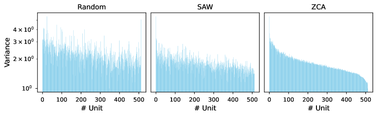
Figure 2: Unit variances after Gram-Schmidt orthogonalization of layer 12 from VGG-16. Prior to the orthogonalization, the units are ordered either randomly (left), using SAW (middle) and using unnormalized-ZCA (right) reordering.

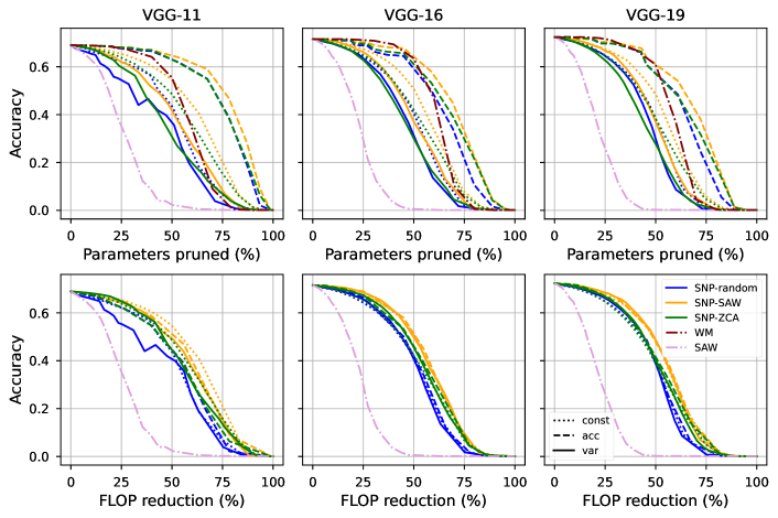
Figure 3: Pruning performance of VGG-11, 16, 19 in the columns from left to right without fine-tuning. Top row: Test accuracy against pruned parameter count. Bottom row: Test accuracy against reduction in FLOPs. We compare the the pre-trained networks organized according to SNP with random order, SAW order and the unnormalized-ZCA order for the heuristics of having a constant pruning ratio for the network (dotted), pruning a percentage of the variances of each layer (solid) or choosing layers according to their performance during layer-wise pruning (dashed). Further, we compare to the SAW method (He et al.,, 2017) and WM (Han et al.,, 2015) in terms of parameter count.

Figure 3 shows the post-pruning accuracies of the VGG11/16/19 networks using the range of methods proposed. When plotting retained accuracy against parameter count, our ‘accuracy’ heuristic outperforms all other methods by some margin, see Appendix A for an analysis of the layer-by-layer accuracies when pruned. Thereafter, the constant pruning ratio consistently performs better than the variance heuristic. In terms of unit ordering, SNP-SAW performs best, followed by the SNP-ZCA and SNP-random. In terms of FLOPs, we see that the variance and constant heuristics catch up to the accuracy heuristic. The biggest difference can again be seen in terms of the reordering. SNP-SAW performs consistently better than SNP-ZCA and SNP-random. In Appendix B, we report the improvement of our variance heuristic method over choosing a fixed pruning ratio in terms of run-time and energy consumption, findings which we expect to translate to savings in CO₂ emissions.

When comparing to different methods, we see that our subspace node perturbation method massively outperform the SAW baseline both in terms of parameter count and FLOPS. Compared to the WM baseline, we observe a major improvement in smaller networks and the ability to retain performance longer at large pruning ratios in larger networks. Note further that the WM method does not immediately translate into a reduced number of FLOPS since it results in sparse but unstructured weight matrices, which cannot be directly utilized to reduce compute load. This would require specialized hardware and/or software, which is why it is not reported in Figure 3.

However, these results also reject our previously made hypothesis, based upon Figure 2, in showing that our ideal ordering by unnormalized ZCA does not translate to best performance. This is despite the much cleaner variance ranking of units which was observed. This suggests that considering the variances of unit activities alone is insufficient in selecting them for pruning.

3.2 ResNet pruning

When pruning ResNets, we observe that even when pruning an entire layer, these networks can retain a great deal of their performance within their skip connections. This is greatly amplified for deeper networks such as ResNet-50 and ResNet-101, as shown in Figure 4 and Appendix C. Overall, we see that our method greatly improves the performance after pruning, even without fine-tuning. However, our expored SNP-ZCA once again appears to have inconsistent advantages over SNP-random. This suggests that units with the smallest activities (variances), which are those pruned by SNP-ZCA, might have an oversized impact upon network behaviour.

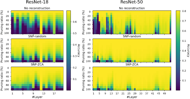
Figure 4: ResNets pruning one layer at a time. Color-coded is the test accuracy. In each subpanel, we show pruning a randomly ordered network without reconstruction (top), SNP with the same random order (middle), and SNP with the ZCA order (bottom).

4 Discussion

In this work, we introduced a novel method for structured pruning on pre-trained deep networks. We proposed to project unit activities into an orthogonal and ranked subspace. When pruning in the subspace, the ranked orthogonalization allows pruning at the node level with an automated reconstruction. We see that this way of pruning in a subspace has favorable implications for unit selection and choice of pruning ratios. This ability to reconstruct pruned unit activations from remaining units allows the extension to and enhancement of other structured pruning methods.

Despite the successes of our method in general, it appears that a view of activity variances as representative of neuron importance is flawed. Our results suggest that the networks communicate important information with even the smallest of activity variances. Therefore, an importance measure that is not only optimizing reconstruction may perform better overall than our SNP-ZCA method. Thankfully our SNP method can be combined with any existing alternative method for node importance ranking.

When pruning whole networks, we found that choosing layers for pruning based upon our ‘accuracy’ heuristic is significantly better than the other heuristics to the different pruning ratios for linear and convolutional layers. Note that this heuristic required an initial step of individually testing the prunability of every single network layer. This method was particularly useful when considering the pruning of parameters, and was less dominant when pruning FLOPs. This observation highlights the differences in methods in prioritising the pruning of dense layers (which contribute significantly to parameter count but not to FLOPs) vs convolutional layers (vice versa). To improve further, we propose to supplement our importance scores with a measure of how sensitive any given layer is to pruning (Molchanov et al.,, 2019). This would attribute appropriate (lower) sensitivity to dense layers at the output of a network and allow these to be prioritised for pruning.

One design choice of our method is that we prune input to a neural network layer. Alternatively, we could decide to prune the pre-activations of layers similar to (Luo et al.,, 2017). The advantage of this would be that it could extend more simply to pruning of certain architectural elements, such as residual connections. Combining input and pre-activation pruning could be a promising route forward for combining these methods.

We focused and restricted ourselves in this work to examining the pruning of trained networks. An extension of this work would be to additionally train networks during and after pruning (fine-tuning). This could be done in a manner by which our orthogonalization method is applied during training to automatically rank unit importances. This could force a network to encode information in a ranked fashion during training and potentially enable far greater pruning performance.

In conclusion, we see the subspace node pruning method described herein as a new perspective on how to view the problem of pruning. This method can be combined with any existing methods for node selection and importance scoring and has the potential to significantly improve any existing node pruning method. However, there also remains some wide open areas to be explored including the application in networks during training and with fine-tuning. Beyond the models investigated here, it also remains to be seen whether pruning approaches can truly impact the most energy-expensive of models, namely transformer models which are currently in vogue.

Appendix A VGG layer analysis

In Figure 3 we observed that a constant pruning ratio outperforms the variance heuristic in terms of parameter count, but not in terms of FLOPs. Here, we analyse this behavior by looking at the variances of each unit in these layers. Figure 5 shows these for the second linear layer VGG-16.

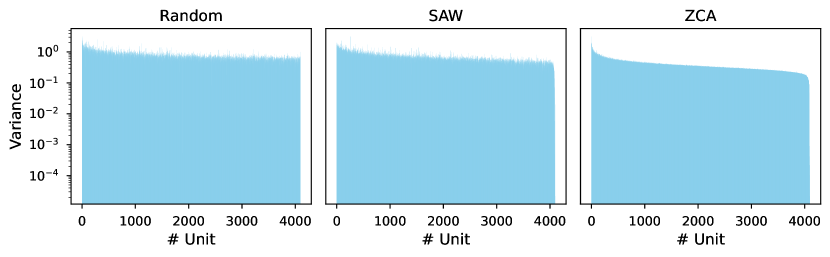
Figure 5: Unit variances after Gram-Schmidt orthogonalization of the second linear layer of VGG-16. Units ordered random (left), SAW (middle) and unnormalized-ZCA(right).

We see that all orders show comparably flat rankings. Such a ranking will result in a pruning behavior similar to the constant heuristic for these layers as variances are spread almost uniformly. Consequently, this prunes a greater ratio in convolutional layers compared to the linear ones.

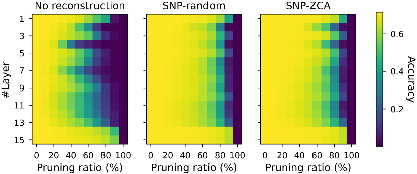
Figure 6: VGG-16: Pruning one layer at a time while keeping all others untouched. The heatmap corresponds to test accuracy.

Figure 6, shows that linear layers are a lot less sensitive to pruning. Compared to the convolutional layers, linear layers are parameter-heavy. Linear layers store a parameter for each input-output connection, whereas convolutional layers use weight sharing to reduce the number of parameters. However, the latter have larger inputs, and perform the same computation on many portions of the input. Therefore, the linear layers have a comparatively stronger impact on parameter count while convolutional have a comparatively stronger impact on the FLOP count. Combining these findings, we see that when pruning the network with a large variance cutoff, the convolutional layers have a comparably much larger pruning ratio than the linear layers, creating an imbalance as seen in Figure 3.

Appendix B Energy consumption analysis

Figure 7 shows the runtime and energy consumption for VGG-16 as a function of test accuracy.

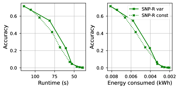
Figure 7: VGG-16 runtime against test accuracy without fine-tuning when using our variance heuristic versus a fixed pruning ratio.

Appendix C ResNet-101

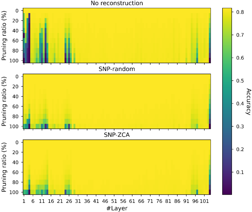
Figure 8: Pruning one layer at a time of ResNet-101. Color-coded is the test accuracy. From top to bottom we see the pruning of the layers with random order without reconstruction, random order and our SNP reconstruction, and the unnormalized-ZCA order with SNP reconstruction.

Appendix D Algorithm including permutations

Below is described the same steps as outlined in the main text, but now including a permutation matrix by which the data could be re-organised prior to subspace node pruning. Note that the permutation matrix is defined based upon any additional importance scoring which is combined with our method.

Input: Data $\mathbf{X}_{l}$, Permutation Matrix $\mathbf{P}_{l}$, Weights $\mathbf{W}_{l}$, Number of units to prune $n$

Output: Pruned weights $\mathbf{\hat{W}}_{l}$

$\mathbf{C}=({\mathbf{P}_{l}\mathbf{X}}_{l})(\mathbf{P}_{l}\mathbf{X}_{l})^{T}$ $\triangleright$ Compute dot-product between (permuted) input feature vectors

$\mathbf{M}^{-1},\mathbf{D}=$ LDL($\mathbf{C}$) $\triangleright$ Decompose matrix $\mathbf{C}$

$\hat{\mathbf{W}}_{l}=\mathbf{W}_{l}\mathbf{P}_{l}^{-1}\mathbf{M}^{-1}_{:,:n}\mathbf{M}_{:n,:n}{\mathbf{P}_{l}}_{:n,*}$ $\triangleright$ Prune $\mathbf{M}$ and $\mathbf{M}^{-1}$ (leading to pruned $\mathbf{W_{l}}$)

$\triangleright$ Note: * indicates non-zero columns only

Return: $\hat{\mathbf{W}}_{l}$

Algorithm 2 Layer-wise subspace node pruning with permutation

References

- Abadi et al., (2015) Abadi, M., Agarwal, A., et al. (2015). TensorFlow: Large-scale machine learning on heterogeneous systems. Software available from tensorflow.org.
- Alvarez and Salzmann, (2016) Alvarez, J. M. and Salzmann, M. (2016). Learning the number of neurons in deep networks. Advances in Neural Information Processing Systems, 29.
- Ayinde et al., (2019) Ayinde, B. O., Inanc, T., and Zurada, J. M. (2019). Redundant feature pruning for accelerated inference in deep neural networks. Neural Networks, 118:148–158.
- Bradbury et al., (2018) Bradbury, J., Frostig, R., Hawkins, P., Johnson, M. J., Leary, C., Maclaurin, D., Necula, G., Paszke, A., VanderPlas, J., Wanderman-Milne, S., and Zhang, Q. (2018). JAX: composable transformations of Python+NumPy programs.
- Bui et al., (2023) Bui, K., Xue, F., Park, F., Qi, Y., and Xin, J. (2023). A proximal algorithm for network slimming. arXiv preprint arXiv:2307.00684.
- Chin et al., (2018) Chin, T.-W., Zhang, C., and Marculescu, D. (2018). Layer-compensated pruning for resource-constrained convolutional neural networks. arXiv preprint arXiv:1810.00518.
- Choquette et al., (2021) Choquette, J., Gandhi, W., Giroux, O., Stam, N., and Krashinsky, R. (2021). Nvidia a100 tensor core gpu: Performance and innovation. IEEE Micro, 41(2):29–35.
- Cuadros et al., (2020) Cuadros, X. S., Zappella, L., and Apostoloff, N. (2020). Filter distillation for network compression. In Proceedings of the IEEE/CVF Winter Conference on Applications of Computer Vision, pages 3140–3149.
- Frankle and Carbin, (2018) Frankle, J. and Carbin, M. (2018). The lottery ticket hypothesis: Finding sparse, trainable neural networks. arXiv preprint arXiv:1803.03635.
- Gao et al., (2019) Gao, S., Liu, X., Chien, L.-S., Zhang, W., and Alvarez, J. M. (2019). Vacl: Variance-aware cross-layer regularization for pruning deep residual networks. In Proceedings of the IEEE/CVF International Conference on Computer Vision Workshops, pages 0–0.
- Gholami et al., (2022) Gholami, A., Kim, S., Dong, Z., Yao, Z., Mahoney, M. W., and Keutzer, K. (2022). A survey of quantization methods for efficient neural network inference. In Low-Power Computer Vision, pages 291–326. Chapman and Hall/CRC.
- Gou et al., (2021) Gou, J., Yu, B., Maybank, S. J., and Tao, D. (2021). Knowledge distillation: A survey. International Journal of Computer Vision, 129(6):1789–1819.
- Han et al., (2015) Han, S., Pool, J., Tran, J., and Dally, W. (2015). Learning both weights and connections for efficient neural network. Advances in Neural Information Processing Systems, 28.
- He et al., (2016) He, K., Zhang, X., Ren, S., and Sun, J. (2016). Deep residual learning for image recognition. In Proceedings of the IEEE Conference on Computer Vision and Pattern Recognition, pages 770–778.
- He et al., (2017) He, Y., Zhang, X., and Sun, J. (2017). Channel pruning for accelerating very deep neural networks. In Proceedings of the IEEE International Conference on Computer Vision, pages 1389–1397.
- Huang and Wang, (2018) Huang, Z. and Wang, N. (2018). Data-driven sparse structure selection for deep neural networks. In Proceedings of the European Conference on Computer Vision (ECCV), pages 304–320.
- Jouppi et al., (2018) Jouppi, N., Young, C., Patil, N., and Patterson, D. (2018). Motivation for and evaluation of the first tensor processing unit. IEEE Micro, 38(3):10–19.
- Krishnamoorthi, (2018) Krishnamoorthi, R. (2018). Quantizing deep convolutional networks for efficient inference: A whitepaper. arXiv preprint arXiv:1806.08342.
- Krizhevsky et al., (2009) Krizhevsky, A., Hinton, G., et al. (2009). Learning multiple layers of features from tiny images.
- Li et al., (2016) Li, H., Kadav, A., Durdanovic, I., Samet, H., and Graf, H. P. (2016). Pruning filters for efficient convnets. arXiv preprint arXiv:1608.08710.
- Liu et al., (2018) Liu, Z., Sun, M., Zhou, T., Huang, G., and Darrell, T. (2018). Rethinking the value of network pruning. arXiv preprint arXiv:1810.05270.
- Luo et al., (2017) Luo, J.-H., Wu, J., and Lin, W. (2017). Thinet: A filter level pruning method for deep neural network compression. In Proceedings of the IEEE International Conference on Computer Vision, pages 5058–5066.
- Molchanov et al., (2019) Molchanov, P., Mallya, A., Tyree, S., Frosio, I., and Kautz, J. (2019). Importance estimation for neural network pruning. In Proceedings of the IEEE/CVF Conference on Computer Vision and Pattern Recognition, pages 11264–11272.
- Molchanov et al., (2016) Molchanov, P., Tyree, S., Karras, T., Aila, T., and Kautz, J. (2016). Pruning convolutional neural networks for resource efficient inference. arXiv preprint arXiv:1611.06440.
- Parikh et al., (2014) Parikh, N., Boyd, S., et al. (2014). Proximal algorithms. Foundations and Trends in Optimization, 1(3):127–239.
- Paszke et al., (2019) Paszke, A., Gross, S., Massa, F., Lerer, A., Bradbury, J., Chanan, G., Killeen, T., Lin, Z., Gimelshein, N., Antiga, L., et al. (2019). Pytorch: An imperative style, high-performance deep learning library. Advances in Neural Information Processing Systems, 32.
- Russakovsky et al., (2015) Russakovsky, O., Deng, J., Su, H., Krause, J., Satheesh, S., Ma, S., Huang, Z., Karpathy, A., Khosla, A., Bernstein, M., et al. (2015). Imagenet large scale visual recognition challenge. International Journal of Computer Vision, 115:211–252.
- Simonyan and Zisserman, (2014) Simonyan, K. and Zisserman, A. (2014). Very deep convolutional networks for large-scale image recognition. arXiv preprint arXiv:1409.1556.
- Wen et al., (2016) Wen, W., Wu, C., Wang, Y., Chen, Y., and Li, H. (2016). Learning structured sparsity in deep neural networks. Advances in Neural Information Processing Systems, 29.
- Ye et al., (2018) Ye, J., Lu, X., Lin, Z., and Wang, J. Z. (2018). Rethinking the smaller-norm-less-informative assumption in channel pruning of convolution layers. arXiv preprint arXiv:1802.00124.
- (31) Zhang, H., Liu, L., Zhou, H., Si, L., Sun, H., and Zheng, N. (2022a). Fchp: Exploring the discriminative feature and feature correlation of feature maps for hierarchical dnn pruning and compression. IEEE Transactions on Circuits and Systems for Video Technology, 32(10):6807–6820.
- (32) Zhang, Y., Yao, Y., Ram, P., Zhao, P., Chen, T., Hong, M., Wang, Y., and Liu, S. (2022b). Advancing model pruning via bi-level optimization. Advances in Neural Information Processing Systems, 35:18309–18326.