eQMARL: Entangled Quantum Multi-Agent Reinforcement Learning for Distributed
Cooperation over Quantum Channels

Abstract

Collaboration is a key challenge in distributed multi-agent reinforcement learning (MARL) environments. Learning frameworks for these decentralized systems must weigh the benefits of explicit player coordination against the communication overhead and computational cost of sharing local observations and environmental data. Quantum computing has sparked a potential synergy between quantum entanglement and cooperation in multi-agent environments, which could enable more efficient distributed collaboration with minimal information sharing. This relationship is largely unexplored, however, as current state-of-the-art quantum MARL (QMARL) implementations rely on classical information sharing rather than entanglement over a quantum channel as a coordination medium. In contrast, in this paper, a novel framework dubbed entangled QMARL (eQMARL) is proposed. The proposed eQMARL is a distributed actor-critic framework that facilitates cooperation over a quantum channel and eliminates local observation sharing via a quantum entangled split critic. Introducing a quantum critic uniquely spread across the agents allows coupling of local observation encoders through entangled input qubits over a quantum channel, which requires no explicit sharing of local observations and reduces classical communication overhead. Further, agent policies are tuned through joint observation-value function estimation via joint quantum measurements, thereby reducing the centralized computational burden. Experimental results show that eQMARL with $\Psi^{+}$ entanglement converges to a cooperative strategy up to $17.8\%$ faster and with a higher overall score compared to split classical and fully centralized classical and quantum baselines. The results also show that eQMARL achieves this performance with a constant factor of $25$-times fewer centralized parameters compared to the split classical baseline.

1 Introduction

Quantum reinforcement learning (QRL) is emerging as a relatively new class of quantum machine learning (QML) for decision making. Exploiting the performance and data encoding enhancements of quantum computing, QRL has many promising applications across diverse areas such as finance [1], healthcare [2], and even wireless networks [3]. Its multi-agent variant, quantum multi-agent reinforcement learning (QMARL), is of specific interest because of the potential synergies between decentralized agent cooperation and quantum entanglement. Indeed, in quantum mechanics [4], entanglement is a distinctly quantum property that intrinsically links the behavior of one particle with another regardless of their physical proximity. The use of entanglement in the broader field of QML is a recent notion. Few core works like [5] and [6] use entangled layers within variational quantum circuit (VQC) designs to link the behavior of quantum bits (or qubits) within a single hybrid quantum model. Even in the recently proposed quantum split learning (QSL) framework [7], entanglement is only used locally within each VQC branch of the quantum split neural network (QSNN) model. What has not yet been explored, however, is using entanglement to couple the behavior of multiple QML models. In QMARL, the use of entanglement can be further extended to the implicit coordination amongst agents during training time. Historically, in both purely classical and quantum multi-agent reinforcement learning (MARL), classical communication, shared replay buffers, centralized global networks, and fully-observable environment assumptions have all proven to be viable methods for coordinating a group policy [8, 9, 10, 11, 12, 13]. Even QSL, which is not exclusive to MARL, relies fully on classical communication between branches of the QSNN [7]. None of these approaches, however, take advantage of the available quantum channel and quantum entanglement as coupling mediums across decentralized agents or model branches, and opt instead for more classical methods of coordination. In short, entanglement is one such phenomenon of quantum mechanics that has not yet been fully explored in the context of cooperation in QMARL settings.

In contrast to prior art, we propose a novel framework dubbed entangled QMARL (eQMARL). The proposed eQMARL is a distributed actor-critic framework, intersecting canonical centralized training with decentralized execution (CTDE) and fully decentralized learning, that facilitates collaboration over a quantum channel using a quantum entangled split critic. Our design uniquely allows agents to coordinate their policies by, for the first time, splitting the quantum critic architecture over a quantum channel and coupling their localized observation encoders using entangled input qubits. This uniquely allows agents to cooperate over a quantum channel, which eliminates the need for observation sharing amongst the agents, and further reduces their classical communication overhead. Also, agent policies are tuned via joint observation-value function estimation using joint quantum measurements across all qubits in the system, which minimizes the computational burden of a central server. As will be evident from our analysis, eQMARL will be shown to converge to a cooperative strategy faster, with higher overall score on average, and with fewer centralized parameters compared to baselines.

1.1 Related works and their limitations

QMARL is a nascent field, with few works applying the quantum advantage to scenarios with multiple agents [8, 9, 10, 11, 12, 13]. Further, the application of quantum to split learning (SL) is even newer, with [7] being the only prior work. In [8] and [9], the authors integrate CTDE into actor-critic QMARL to train localized quantum actors with a centralized quantum critic. In [10], the authors propose a quantum meta MARL framework which uses a central meta Q-learning agent to train other local agents. The work in [11] proposes quantum asynchronous advantage actor-critic as a framework for training decentralized QRL agents, which leverages jointly a global shared memory and agent-specific memories to train parallel agents. The work in [12] proposes a QMARL approach for autonomous mobility cooperation using actor-critic networks with CTDE in noisy intermediate-scale quantum (NISQ) environments with a shared replay buffer. In [13], the authors propose a QMARL approach using evolutionary optimization with a VQC design based on quantum classification networks and agent policies implemented as independent VQC models with shared local information. Finally, in [7], the authors propose an extension of SL to QML for classification tasks; where local QNN branches send predictions via a classical channel to a central server for cross-channel pooling aggregation.

The resounding theme in [8, 9, 10, 11, 12, 13, 7] is the use of independent agents or branches that communicate and learn through centralized classical means. No prior work [8, 9, 10, 11, 12, 13, 7], however, makes use of the quantum channel as a medium for coupling system elements or for multi-agent collaboration. In [8, 9, 10, 11, 12, 13, 7], the quantum elements serve as drop-in replacements for classical neural network (NN) counterparts, and, importantly, the quantum channel between agents and the potential for sharing entangled qubit states go largely under-utilized. Simply put, entanglement and the quantum channel are potentially useful untapped cooperative resources intrinsic to QMARL that have largely unknown benefits.

1.2 Contributions

The contributions of this work are summarized as follows:

• We propose a novel eQMARL framework that trains decentralized policies via a split quantum critic over a quantum channel with entangled input qubits and joint measurement.

• We propose a new QMARL algorithm for training distributed agents via optimizing a split critic without sharing local environment observations amongst agents or a central server.

• We show that the split nature of eQMARL reduces the computational burden of a central quantum server by distributing and tuning parameterized quantum gates across agents in the system, and requiring a small number of parameters for joint measurement.

• We empirically demonstrate that eQMARL with $\Psi^{+}$ entanglement exhibits a faster convergence time that can reach up to $17.8\%$ faster, and with higher overall score, compared to split classical and fully centralized classical and quantum baselines in environments with full and partial information. Further, the results also show that eQMARL achieves this level of performance and cooperation with a constant factor of $25$-times fewer centralized parameters compared to the split classical baseline.

To the best of our knowledge, this is the first application of QMARL that exploits the quantum channel and entanglement between agents to learn without sharing local observations, while also reducing the classical communication overhead and central computation burden of leading approaches.

The rest of this paper is organized as follows. In Section 2, we provide preliminary information that benefits our discussions. In Section 3, we discuss our proposed eQMARL framework in detail. In Section 4, we detail our experiments and discuss results. Finally, conclusions are drawn in Section 5.

2 Preliminaries

2.1 Quantum multi-agent reinforcement learning

We consider a reinforcement learning (RL) setting with multiple agents in environments with both full and partial information. The dynamics of a system with full information is described by a Markov game with an underlying Markov decision process (MDP) with tuple $M_{\textrm{MDP}}=\langle\mathcal{N},\mathcal{S},\mathcal{A},\mathcal{P},\mathcal{R}\rangle$ where $\mathcal{N}$ is a set of $N$ agents, $\mathcal{S}=\{\mathcal{S}^{n}\}_{n\in\mathcal{N}}$ is the set of joint states across all agents, $\mathcal{A}=\{\mathcal{A}^{(n)}\}_{n\in\mathcal{N}}$ is the set of joint actions, $\mathcal{S}^{(n)}$ and $\mathcal{A}^{(n)}$ are the set of states and actions for agent $n$, $\mathcal{P}(s_{t+1}|s_{t},a_{t})$ is the state transition probability, and $\mathcal{R}(s_{t},a_{t})=\{r^{(n)}_{t}\}_{n\in\mathcal{N}}\in\mathbb{R}^{N}$ is the joint reward $\forall s_{t}\in\mathcal{S},a_{t}\in\mathcal{A}$. The dynamics of a system with partial information is described by a Markov game with an underlying partially observable MDP (POMDP) with tuple $M_{\textrm{POMDP}}=\langle\mathcal{N},\mathcal{S},\mathcal{A},\mathcal{P},\mathcal{R},\Omega,\mathcal{O}\rangle$ where $\mathcal{N},\mathcal{S},\mathcal{A},\mathcal{P}$ are the same as in $M_{\textrm{MDP}}$, however the full state of the environment $s_{t}$ at time $t$ is kept hidden from the players. Instead, at time $t$ the agents receive a local observation from the set of joint observations $\Omega=\{\Omega^{(n)}\}_{n\in\mathcal{N}}$, where $\Omega^{(n)}$ is the set of observations for agent $n$, with transition probability $\mathcal{O}(o_{t}|s_{t+1},a_{t})$, $\forall o_{t}\in\Omega$, which is dependent on the hidden environment state after taking a joint action. We treat $M_{\textrm{MDP}}$ as a special case of $M_{\textrm{POMDP}}$ where $o^{(n)}_{t}=s^{(n)}_{t}$, that is the observations represent the full environment state information. Hereinafter, all notations will use $o^{(n)}_{t}$ in place of the local environment state for brevity to encompass all cases.

QMARL is the application of quantum computing to MARL. A popular approach in MARL is through actor-critic architectures, which tune policies, called actors, via an estimator for how good or bad the policy is at any given state of an environment, called a critic. To do this, the critic needs access to the local agent environment observations to estimate the value for a particular environment state. Current state of the art approaches follow the CTDE framework which deploys the critic on a central server and the actors across decentralized agents. Because the critic and the agents are physically separated, CTDE requires the agents to transmit their local observations to the server for the critic to estimate the joint value, thereby publicizing potentially private local observations. Quantum is often integrated as a drop-in replacement for classical NNs, called VQCs, within many MARL systems. These trainable quantum circuits tune the state of qubits, the quantum analog of classical bits, using unitary gate operations.

2.2 Quantum computation

2.2.1 Qubit states

The state of a qubit is represented as a 2-dimensional unit vector in complex Hilbert space $\mathcal{H}\in\mathbb{C}^{2}$. The computational basis is the set of states $\left\{\ket{0}=\begin{bmatrix}1&0\end{bmatrix}^{T},\ket{1}=\begin{bmatrix}0&1\end{bmatrix}^{T}\right\}$ which forms a complete and orthonormal basis in $\mathcal{H}$ (meaning $\innerproduct{0}{1}=\innerproduct{1}{0}=0$ and $\innerproduct{0}{0}=\innerproduct{1}{1}=1$). All qubit states can be expressed as a linear combination of any complete and orthonormal basis, such as the computational basis, which is called superposition. We adopt Dirac notation to describe arbitrary qubit states $\ket{\psi}=\begin{bmatrix}\alpha&\beta\end{bmatrix}^{T}=\alpha\ket{0}+\beta\ket{1}\in\mathcal{H}$ (called “ket psi”) where $|\alpha|^{2}+|\beta|^{2}=1$, their conjugate transpose $\bra{\psi}=\ket{\psi}^{\dagger}=\begin{bmatrix}\alpha^{*}&\beta^{*}\end{bmatrix}=\alpha^{*}\bra{0}+\beta^{*}\bra{1}$ (called “bra psi”), the inner product $\innerproduct{\psi_{1}}{\psi_{2}}=\alpha_{1}^{*}\alpha_{2}+\beta_{1}^{*}\beta_{2}$, and the outer product $\outerproduct{\psi_{1}}{\psi_{2}}=\begin{bmatrix}\alpha_{1}\alpha_{2}^{*}&\alpha_{1}\beta_{2}^{*}\\ \beta_{1}\alpha_{2}^{*}&\beta_{1}\beta_{2}^{*}\end{bmatrix}$. Quantum systems with $D$ qubits can also be represented by extending the above notation using the Kronecker (tensor) product where $\mathcal{H}=\bigotimes_{d=0}^{D-1}\mathcal{H}_{d}=(\mathbb{C}^{2})^{\otimes D}$ is the complex space of the system state $\ket{\psi}=\bigotimes_{d=0}^{D-1}\ket{\psi_{d}}$ for all $\ket{\psi_{D}}\in\mathcal{H}_{D}$. States that can be represented as either a single ket vector, or a sum of basis states are called pure states. For example, $\ket{0}$, $\ket{1}$, and $\frac{1}{\sqrt{2}}(\ket{0}+\ket{1})$ are all pure states in $\mathcal{H}$.

2.2.2 Quantum gates

A quantum gate is an unitary operator (or matrix) $U$, such that $UU^{\dagger}=\mathbb{I}$, where $\mathbb{I}$ is the identity matrix, acting on the space $\mathcal{H}$ which maps between qubit states. Here, we use the single-qubit Pauli gates $X=\begin{bmatrix}0&1\\ 1&0\end{bmatrix}$, $Y=\begin{bmatrix}0&-i\\ i&0\end{bmatrix}$, and $Z=\begin{bmatrix}1&0\\ 0&-1\end{bmatrix}$, their parameterized rotations $R_{X}(\theta)=e^{-i\frac{\theta}{2}X}$, $R_{Y}(\theta)=e^{-i\frac{\theta}{2}Y}$, and $R_{Z}(\theta)=e^{-i\frac{\theta}{2}Z}$ where $\theta\in\mathbb{R}[0,2\pi]$, the Hadamard gate $H=\frac{1}{\sqrt{2}}\begin{bmatrix}1&1\\ 1&-1\end{bmatrix}$, the 2-qubit controlled-$X$ gate ${CX}_{1,2}=\begin{bmatrix}\mathbb{I}&\bm{0}\\ \bm{0}&X\end{bmatrix}$ (also called CNOT), and the controlled-$Z$ gate ${CZ}_{1,2}=\begin{bmatrix}\mathbb{I}&\bm{0}\\ \bm{0}&Z\end{bmatrix}$, where $\mathbb{I}$ is the identity matrix and $\bm{0}$ is a square matrix of zeros.

2.2.3 Entanglement

Consider two arbitrary quantum systems $A$ and $B$, represented by Hilbert spaces $\mathcal{H}_{A}$ and $\mathcal{H}_{B}$. We can represent the Hilbert space of the combined system using the tensor product $\mathcal{H}_{A}\otimes\mathcal{H}_{B}$. If the quantum states of the two systems are $\ket{\psi}_{A}$ and $\ket{\psi}_{B}$, then the state of the combined system can be represented as $\ket{\psi}_{A}\otimes\ket{\psi}_{B}$. Quantum states that can be cleanly represented in this form, i.e., separated by tensor product, are said to be separable. Not all quantum states, however, are separable. For example, if we fix a set of basis states $\left\{\ket{0}_{A},\ket{1}_{A}\right\}\in\mathcal{H}_{A}$ and $\left\{\ket{0}_{B},\ket{1}_{B}\right\}\in\mathcal{H}_{B}$, then a general state in the space of $\mathcal{H}_{A}\otimes\mathcal{H}_{B}$ can be represented as $\ket{\psi}=\sum_{a\in\{0,1\}}\sum_{b\in\{0,1\}}c_{a,b}\ket{a}_{A}\otimes\ket{b}_{B},$ which is separable if there $c_{a,c}=c_{a}c_{b}$, $\forall a,b\in\{0,1\}$, producing the isolated states $\ket{\psi}_{A}=\sum_{a\in\{0,1\}}c_{a}\ket{a}_{A}$ and $\ket{\psi}_{B}=\sum_{b\in\{0,1\}}c_{b}\ket{b}_{B}$. If, however, there exists one $c_{a,c}\neq c_{a}c_{b}$, then the combined state is inseparable. In such cases, if a state is inseparable, it is said to be entangled.

The four Bell states $\mathcal{B}=\left\{\ket{\Phi^{+}}_{AB},\ket{\Phi^{-}}_{AB},\ket{\Psi^{+}}_{AB},\ket{\Psi^{-}}_{AB}\right\}$ form a complete basis for two-qubit systems $\mathcal{H}_{A}\otimes\mathcal{H}_{B}$, and have the form: $\ket{\Phi^{+}}_{AB}=\frac{1}{\sqrt{2}}\left(\ket{0}_{A}\ket{0}_{B}+\ket{1}_{A}\ket{1}_{B}\right)$, $\ket{\Phi^{-}}_{AB}=\frac{1}{\sqrt{2}}\left(\ket{0}_{A}\ket{0}_{B}-\ket{1}_{A}\ket{1}_{B}\right)$, $\ket{\Psi^{+}}_{AB}=\frac{1}{\sqrt{2}}\left(\ket{0}_{A}\ket{1}_{B}+\ket{1}_{A}\ket{0}_{B}\right)$, and $\ket{\Psi^{-}}_{AB}=\frac{1}{\sqrt{2}}\left(\ket{0}_{A}\ket{1}_{B}-\ket{1}_{A}\ket{0}_{B}\right)$. Since it is impossible to separate the states of $\mathcal{B}$ into individual systems $\mathcal{H}_{A}$ and $\mathcal{H}_{B}$, the four Bell states are entangled. In particular, the Bell states are pure entangled states of the combined system $\mathcal{H}_{A}\otimes\mathcal{H}_{B}$, but cannot be separated into pure states of systems $\mathcal{H}_{A}$ and $\mathcal{H}_{B}$.

2.2.4 Projective measurements and observables

A projective measurement is a Hermitian and unitary operator $O$, such that $O=O^{\dagger}$ and $OO^{\dagger}=\mathbb{I}$, called an observable. The outcomes of a measurement are defined by an observable’s spectral decomposition $O=\sum_{m=0}^{M-1}\lambda_{m}P_{m}$, where $M=2^{D}$ represents the number of measurement outcomes for $D$ qubits, and $m$ is a specific measurement outcome in terms of eigenvalues $\lambda_{m}$ and orthogonal projectors $P_{m}$ in the respective eigenspace. According to the Born rule [14, 15, 16], the outcome of measuring an arbitrary state $\ket{\psi}$ will be one of the eigenvalues $\lambda_{m}$, and the state will be projected using the operator $P_{m}/\sqrt{p(m)}$ with probability $p(m)=\bra{\psi}P_{m}\ket{\psi}=\expectationvalue{P_{m}}_{\psi}$. The expected value of the observable with respect to the arbitrary state $\ket{\psi}$ is given by $\mathbb{E}_{\psi}[O]=\sum_{m=0}^{M-1}\lambda_{m}p(m)=\expectationvalue{O}_{\psi}$.

2.2.5 Commuting observables

A set of observables $\{O_{1},\dots,O_{K}\}$ share a common eigenbasis (i.e., a common set of eigenvectors with unique eigenvalues) if $[O_{i},O_{j}]=O_{i}O_{j}-O_{j}O_{i}=0$, $\forall i,j\in[1,K]$, i.e., their pair-wise commutator is zero. In such cases the observables in the set are said to be pair-wise commuting, which in practice means that all observables in the set can be measured at the same time.

3 Proposed eQMARL framework

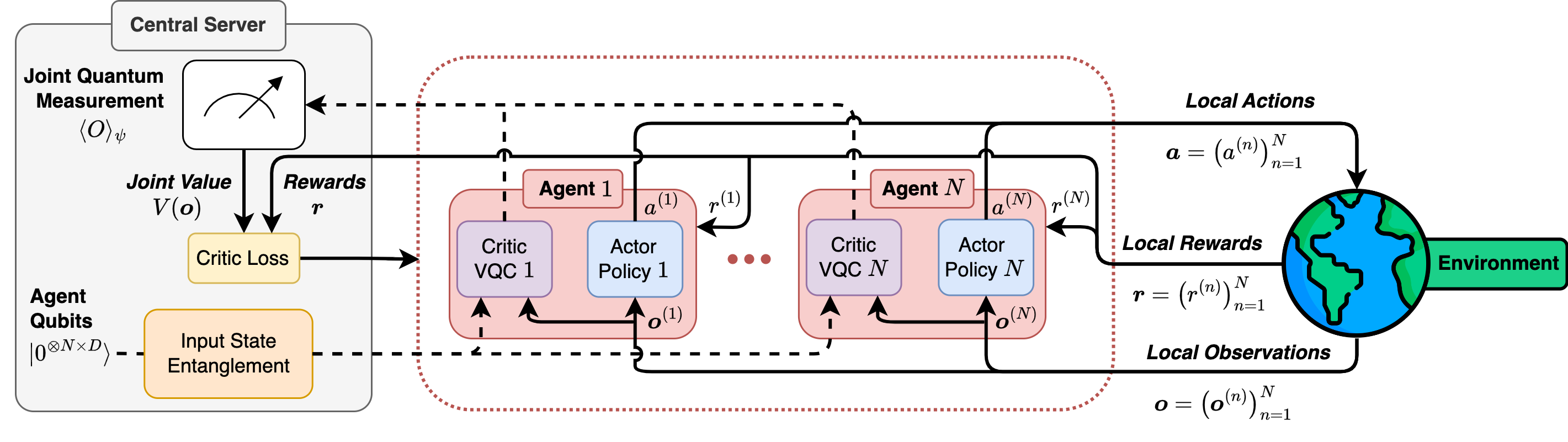
Figure 1: General design of our eQMARL framework. Dashed (solid) arrows represent quantum (classical) communication. A split quantum critic is deployed across the agents via local VQCs (purple) coupled via input entanglement (orange) at a trusted central server (gray). Joint quantum measurements across all qubits (white) estimate the joint value from the locally-encoded observations.

Our proposed eQMARL framework is a new approach for training multi-agent actor-critic architectures which lies at the intersection between CTDE and fully decentralized learning. Inspired from CTDE, we deploy decentralized agent policies which learn using a joint value function at training time. The key to our approach, however, is that we use quantum entanglement to deploy the joint value function estimator as a critic network which is spread across the agents to operate in mostly decentralized fashion. An overview of our framework design is shown in Fig. 1, and the design of the system architecture from a purely quantum perspective is shown in Fig. 2. From Fig. 1, the two main elements of eQMARL are a central quantum server and a set of $N$ decentralized quantum agents $\mathcal{N}=\{n\}_{n=1}^{N}$. The decentralized agents do not communicate with each other; only communication with the server is necessary during training. During execution, the agents interact with the environment independently and are fully decentralized. During training, our eQMARL framework is divided into core stages: 1) Centralized quantum input state entanglement preparation, 2) Decentralized agent environment observation encoding and variational rotations, and 3) Joint value estimation through joint quantum measurement. Fig. 2 shows how input states are prepared using custom pairwise entanglement operators, followed by agent VQCs, and then joint measurements. Physically, these operations occur at different locations, however, it is equivalent to consider these as a single quantum system, from input state preparation to final measurement. For purposes of quantum state transmission, we assume an ideal quantum channel environment with no losses.

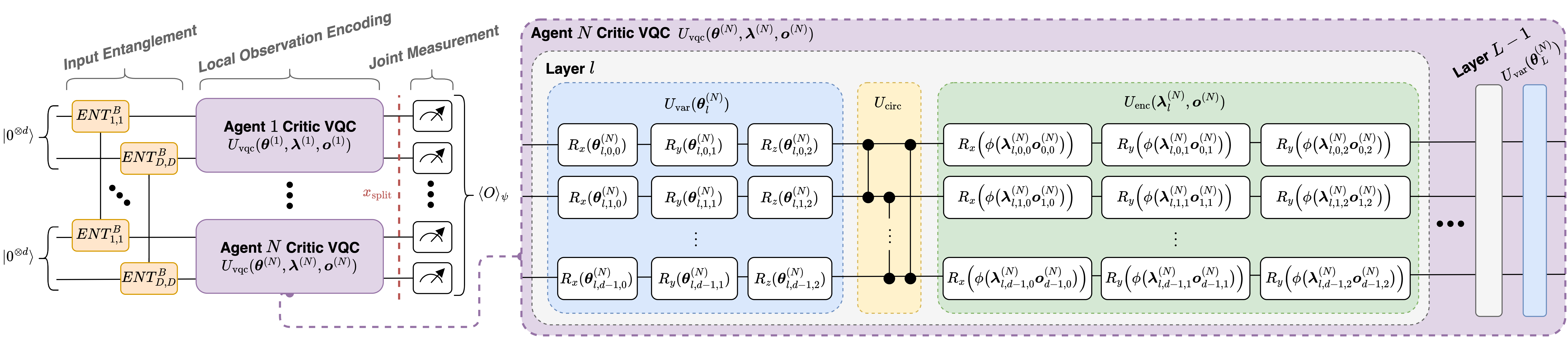
Figure 2: Quantum system design with $N$ agents and $D$ qubits per agent. Input entanglement operators (orange) couple the split critic VQCs (purple, with split point marked in red), which has cascaded layers of variational (blue), circular entanglement (yellow), and encoding (green) operators.

3.1 Joint input entanglement

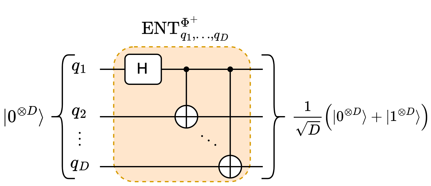
(a) $\Phi^{+}$

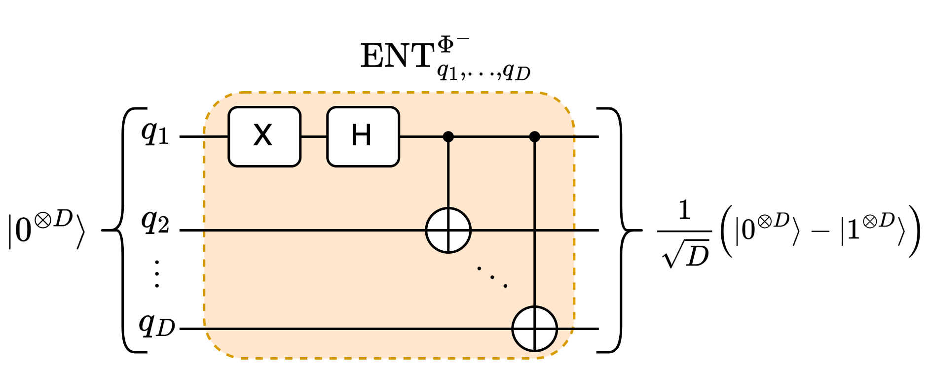
(b) $\Phi^{-}$

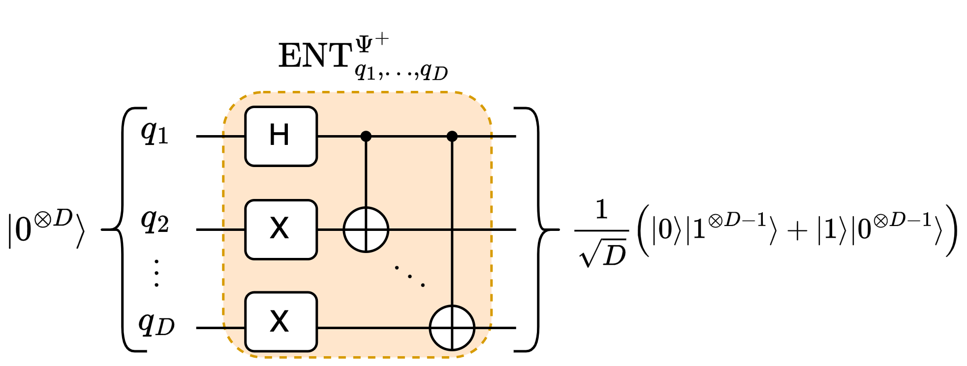
(c) $\Psi^{+}$

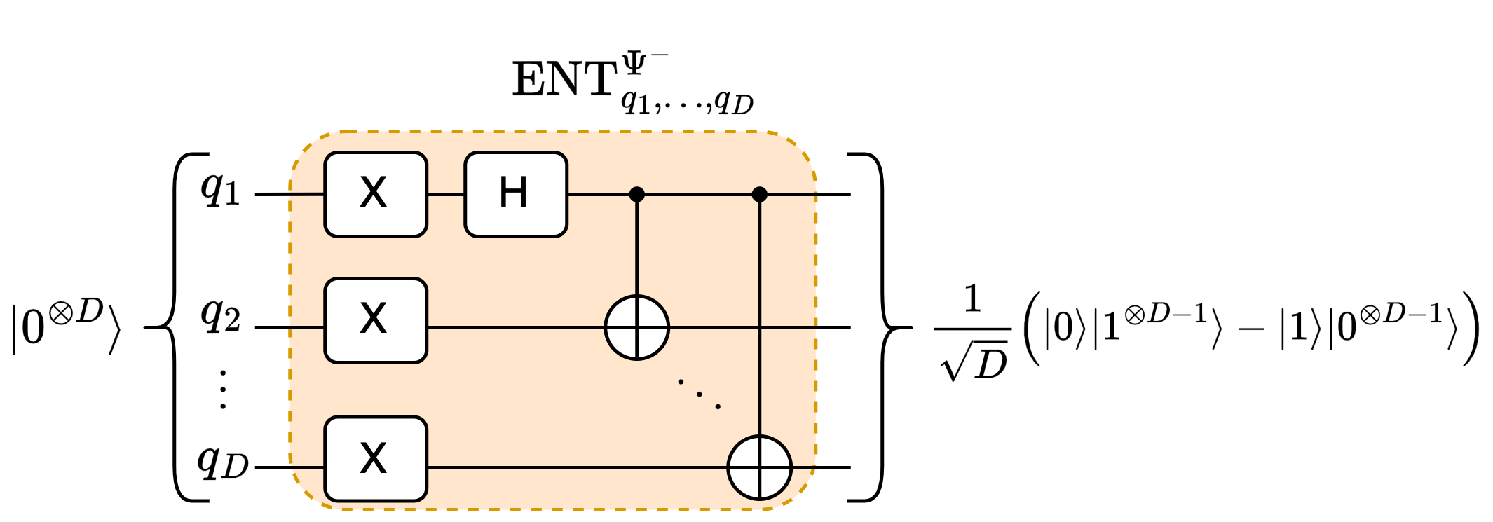
(d) $\Psi^{-}$

Figure 3: Joint entanglement operator circuits for Bell states (a) $\Phi^{+}$, (b) $\Phi^{-}$, (c) $\Psi^{+}$, and (d) $\Psi^{-}$.

The first stage of eQMARL creates an entangled input state for the split quantum critic network, which couples the critic VQCs spread across the agents. Each agent $n\in\mathcal{N}$ is assigned a set of $D$ qubits $\mathcal{Q}^{(n)}=\{q_{d}^{(n)}\}_{d=1}^{D}$ chosen based upon the environment state dimension and desired quantum state encoding method. The number of qubits is $N\times D$, and is represented by the union of agent qubit sets $\mathcal{Q}=\bigcup_{n=1}^{N}\mathcal{Q}^{(n)}$. We couple the agents by preparing an input state which pairwise entangles their qubits. Without loss of generality, we create a variation of Bell state entanglement [17]. Hence, the entanglement scheme is based on the set of Bell states $\mathcal{B}\in\{\Phi^{+},\Phi^{-},\Psi^{+},\Psi^{-}\}$ such that

$$\textrm{ENT}^{B}_{\delta(1,d),\dots,\delta(N,d)}=\begin{cases}\bigl{(}\bigotimes_{n=2}^{N}\textrm{CNOT}_{\delta(1,d),\delta(n,d)}\bigr{)}H_{\delta(1,d)},&\textrm{if $B=\Phi^{+}$},\\[5.0pt] \bigl{(}\bigotimes_{n=2}^{N}\textrm{CNOT}_{\delta(1,d),\delta(n,d)}\bigr{)}H_{\delta(1,d)}X_{\delta(1,d)},&\textrm{if $B=\Phi^{-}$},\\[5.0pt] \bigl{(}\bigotimes_{n=2}^{N}\textrm{CNOT}_{\delta(1,d),\delta(n,d)}\bigr{)}H_{\delta(1,d)}\bigl{(}\bigotimes_{k=2}^{N}X_{\delta(k,d)}\bigr{)},&\textrm{if $B=\Psi^{+}$},\\[5.0pt] \bigl{(}\bigotimes_{n=2}^{N}\textrm{CNOT}_{\delta(1,d),\delta(n,d)}\bigr{)}H_{\delta(1,d)}\bigl{(}\bigotimes_{k=1}^{N}X_{\delta(k,d)}\bigr{)},&\textrm{if $B=\Psi^{-}$},\end{cases}$$ (1)

is a coupling operator that creates Bell state entanglement across qubits $\{q^{(n)}_{d}\}_{n=1}^{N}\subseteq\mathcal{Q}$, where $\delta(n,d)=(n-1)D+d$ is an index mapping within $\mathcal{Q}$ for agent $n\in\mathcal{N}$ at qubit index $d\in[1,D]$, i.e., $\delta(n,d)\equiv q^{(n)}_{d}\in\mathcal{Q}^{(n)}$, and $B\in\mathcal{B}$ represents the scheme of entanglement. Importantly, this operator can be applied to entangle any arbitrary set of qubits within the circuit. Note that in this work we assume the agents receive their entangled qubits in real-time via a trusted central source, i.e., a central server, however, they could be pre-generated and stored in quantum memory at the agent if desired. The quantum circuits that generate each $B\in\mathcal{B}$ are shown in Fig. 3.

3.2 Decentralized split critic VQC design

At its core, our joint quantum critic is a split neural network (SNN) [18], with each agent’s local VQC serving as a branch. After the input qubits are entangled, they are partitioned back into $N$ sets of $D$ qubits, i.e., $\{\mathcal{Q}^{(n)}\}_{n\in\mathcal{N}}$, and transmitted to each agent respectively. The agents collect and encode local observations from the environment into their assigned qubits using a VQC. We use the VQC architectures of [19, 20] for our hybrid quantum network design. Each agent in our QMARL setting uses the same VQC architecture for their branch of the critic, but tunes their own unique set of parameters. The same architecture is a reasonable assumption since all agents are learning in the same environment, and the uniqueness of parameters tailors each branch to local observations. From Fig. 2, the VQC design consists of $L$ cascaded layers of variational, circular entanglement, and encoding operators, with an additional variational layer at the end of the circuit before measurement. The trainable variational layer performs sequential parameterized Pauli X, Y, and Z-axis rotations, and it can be expressed as the unitary operator $U_{\textrm{var}}(\bm{\theta}^{(n)}_{l})=\bigotimes_{d=0}^{D-1}R_{z}(\bm{\theta}^{(n)}_{l,d,2})R_{y}(\bm{\theta}^{(n)}_{l,d,1})R_{x}(\bm{\theta}^{(n)}_{l,d,0}),$ where $\bm{\theta}^{(n)}\in[0,2\pi]^{(L+1)\times D\times 3}$ is a matrix of rotation angle parameters for agent $n$. The non-trainable circular entanglement layer binds neighboring qubits within a single agent using the operator $U_{\textrm{circ}}=CZ_{0,D-1}\bigl{(}\prod_{d=0}^{D-2}CZ_{d,d+1}\bigr{)}.$ The trainable encoding layer maps a matrix of classical features $\bm{o}^{(n)}\in\mathbb{R}^{D\times 3}$, i.e., an agent’s environment observation, into a quantum state via the operator: $U_{\textrm{enc}}(\bm{\lambda}^{(n)}_{l},\bm{o}^{(n)})=\bigotimes_{d=0}^{D-1}R_{z}\bigl{(}\phi\bigl{(}\bm{\lambda}^{(n)}_{l,d,2}\bm{o}^{(n)}_{d,2}\bigr{)}\bigr{)}R_{y}\bigl{(}\phi\bigl{(}\bm{\lambda}^{(n)}_{l,d,1}\bm{o}^{(n)}_{d,1}\bigr{)}\bigr{)}R_{x}\bigl{(}\phi\bigl{(}\bm{\lambda}^{(n)}_{l,d,0}\bm{o}^{(n)}_{d,0}\bigr{)}\bigr{)},$ where $\bm{\lambda}^{(n)}\in\mathbb{R}^{L\times D\times 3}$ is a matrix of trainable scaling parameters, and $\phi\colon\mathbb{R}\mapsto\mathbb{R}$ is an optional squash activation function. The entire VQC can be expressed as a single operator, as follows:

$$U_{\textrm{vqc}}(\bm{\theta}^{(n)},\bm{\lambda}^{(n)},\bm{o}^{(n)})=U_{\textrm{var}}(\bm{\theta}^{(n)}_{L})\prod_{l=0}^{L-1}U_{\textrm{enc}}(\bm{\lambda}^{(n)}_{L-l-1},\bm{o}^{(n)})~{}U_{\textrm{circ}}~{}U_{\textrm{var}}(\bm{\theta}^{(n)}_{L-l-1}),$$ (2)

which is parameterized by variational angles $\bm{\theta}^{(n)}$ and encoding weights $\bm{\lambda}^{(n)}$.

3.3 Centralized joint measurement

The locally encoded qubits for each agent are subsequently forwarded to a central quantum server, which could either be the entanglement source or a different location, for joint measurement. A joint measurement across all qubits in the system is made in the Pauli $Z$ basis using the observable $O=\bigotimes_{d=1}^{N\times D}Z_{d}$. The joint value for the locally-encoded observations is then estimated as follows:

$$V(\bm{o})\simeq w\left(\frac{1+\langle O\rangle_{\psi}}{2}\right),$$ (3)

where $w\in\mathbb{R}$ is a learned scaling parameter, $\langle O\rangle_{\psi}$ is the expected value of the joint observable w.r.t. an arbitrary system state $\ket{\psi}$ across all qubits, and $\bm{o}=(\bm{o}^{(n)})_{n=1}^{N}$ is a vector of joint observations. This rescaling is necessary because the range of the measured observable is $\langle O\rangle_{\psi}\in[-1,1]$ (i.e., proportional to the eigenvalues of the operator $O$), whereas $V(\bm{o})\in\mathbb{R}$. The critic loss with respect to the joint value and local agent rewards is then disseminated amongst the agents for tuning of their localized portion of the split critic network and local policy networks.

3.4 Split critic loss

The loss of the split critic is derived in a way similar to [18]. Since the input entanglement stage of eQMARL has no trainable parameters, it does not exist for the purposes of SL backpropagation. We denote the point of joint quantum measurement as the split point, which is preceded by local agent VQC branches. Each branch can be individually tuned using the partial gradient of the loss at the split point via partial gradient w.r.t. its own local parameters. If we define $x_{\textrm{split}}$ as the split point, then the partial gradient of each branch’s parameters can be estimated using the central loss, as follows:

$$\nabla_{\bm{\theta}_{\textrm{critic}}^{(n)}}\mathcal{L}_{\textrm{critic}}=\frac{\partial\mathcal{L}_{\textrm{critic}}}{\partial\bm{\theta}_{\textrm{critic}}^{(n)}}=\frac{\partial\mathcal{L}_{\textrm{critic}}}{\partial x_{\textrm{split}}}\frac{\partial x_{\textrm{split}}}{\partial\bm{\theta}_{\textrm{critic}}^{(n)}}=\underbrace{\left(\nabla_{x_{\textrm{split}}}\mathcal{L}_{\textrm{critic}}\vphantom{\left(\nabla_{\bm{\theta}_{\textrm{critic}}^{(n)}}x_{\textrm{split}}\right)}\right)}_{\textrm{Central server}}\underbrace{\left(\nabla_{\bm{\theta}_{\textrm{critic}}^{(n)}}x_{\textrm{split}}\right)}_{\textrm{Local agent}},$$ (4)

where $\nabla_{x_{\textrm{split}}}\mathcal{L}_{\textrm{critic}}$ is the gradient of the loss at the split point, and $\nabla_{\bm{\theta}_{\textrm{critic}}^{(n)}}x_{\textrm{split}}$ is the gradient from the split point back to the start of branch $n\in\mathcal{N}$. The value of $\nabla_{x_{\textrm{split}}}\mathcal{L}_{\textrm{critic}}$ is sent classically to the agents, and since Eq. 3 only uses a single trainable parameter, $w$, the classical communication overhead needed for split backpropagation is minimal. Here, we use the Huber loss for the critic

$$\mathcal{L}_{\textrm{critic}}=\frac{1}{T-1}\sum_{\tau=0}^{T-1}\begin{cases}\frac{1}{2}(V(\bm{o}_{\tau})-Q(\bm{o}_{\tau},\bm{a}_{\tau}))^{2}&\textrm{if $V(\bm{o}_{\tau})-Q(\bm{o}_{\tau},\bm{a}_{\tau})\leq\delta$},\\[5.0pt] \delta|V(\bm{o}_{\tau})-Q(\bm{o}_{\tau},\bm{a}_{\tau})|-\frac{1}{2}\delta^{2}&\textrm{otherwise},\end{cases}$$ (5)

where $\delta$ controls the point in which the loss function turns from quadratic to linear. In this work we use $\delta=1$. For the actors, we deploy policy sharing amongst the agents. As such, all agents us the same policy parameters, and thus the loss must aggregate the individual losses of each agent. We train using the entropy-regularized advantage function

$$\mathcal{L}_{\textrm{actor}}=\frac{1}{n(T-1)}\sum_{n=1}^{N}\sum_{\tau=0}^{T-1}\Big{[}-A(o^{(n)}_{\tau},a^{(n)}_{\tau})\log_{e}{p(a^{(n)}_{\tau})}+\alpha H(a^{(n)}_{\tau})\Big{]},$$ (6)

where $H(a^{(n)}_{\tau})=-p(a^{(n)}_{\tau})\log_{e}{p(a^{(n)}_{\tau})}$ is the entropy of selecting an action, $\alpha$ controls the influence of entropy, $n\in\mathcal{N}$ is the agent index, and $p(a^{(n)}_{\tau})$ is the probability of chosen action at time step $\tau$.

3.5 Coupled agent learning algorithm

Require: Set of $N$ agents $\mathcal{N}$, 1 quantum entanglement source, and 1 quantum measurement server

1 Initialize $N$ agent actor networks with shared parameters $\bm{\theta}_{\textrm{actor}}$ and local replay buffer $\mathcal{D}^{(n)}=\{\}$, $\forall n\in\mathcal{N}$;

2 Initialize $N$ critic branches $U_{\textrm{vqc}}$ with $D$ qubits and parameters $\bm{\theta}_{\textrm{critic}}^{(n)}$, $\bm{\lambda}^{(n)}$, $\forall n\in\mathcal{N}$;

3 for episode=1, MaxEpisode do

       $\triangleright$ Localized environment interaction.

4       $t=0$;

5       $done=False$;

6       while $done\neq True$ and $t<max\ steps$ do

7             for each agent $n\in\mathcal{N}$ do

8                   Get local observation $\bm{o}_{t}^{(n)}$ from environment;

9                   Compute $\pi_{\bm{\theta}_{\textrm{actor}}^{(n)}}(a|\bm{o}_{t}^{(n)})$ and sample $a_{t}^{(n)}$;

10                   Apply action $a_{t}^{(n)}$ and get reward $r_{t}^{(n)}$ and next observation $\bm{o}_{t+1}^{(n)}$;

11                   Update local replay buffer $\mathcal{D}^{(n)}=\mathcal{D}^{(n)}\cup\left\{\left(\bm{o}_{t}^{(n)},a_{t}^{(n)},r_{t}^{(n)},\bm{o}_{t+1}^{(n)}\right)\right\}$;

12                   If $\bm{o}_{t+1}^{(n)}$ is terminal then communicate $done=True$;

13                  

14             end for

15            $t=t+1$;

16            

17       end while

       $\triangleright$ eQMARL framework for training.

18       for $\tau\in[0,t-2]$ do

19             Central quantum server generates $2N$ sets of $D$ entangled qubits and transmits to agents via quantum channel (could be prepared a priori and stored in quantum memory);

20             for each agent $n\in\mathcal{N}$ do

21                   Apply $U_{\textrm{vqc}}(\bm{\theta}^{(n)}_{\textrm{critic}},\bm{\lambda}^{(n)},\bm{o}_{\tau}^{(n)})$ and $U_{\textrm{vqc}}(\bm{\theta}^{(n)}_{\textrm{critic}},\bm{\lambda}^{(n)},\bm{o}_{\tau+1}^{(n)})$ from Eq. 2 locally using assigned entangled input qubits;

22                   Transmit via quantum channel the qubits after applying $U_{\textrm{vqc}}$ to central quantum server;

23                   Transmit via classical channel the reward $r_{\tau}^{(n)}$ and action $a_{\tau}^{(n)}$ at the current time step to central quantum server (only reward if policy sharing is not used);

24                  

25             end for

            $\triangleright$ Using notation $\bm{o}_{\tau}=\bigl{(}\bm{o}_{\tau}^{(n)}\bigr{)}_{n=1}^{N}$, $\bm{o}_{\tau+1}=\bigl{(}\bm{o}_{\tau+1}^{(n)}\bigr{)}_{n=1}^{N}$, $\bm{a}_{\tau}=\bigl{(}a_{\tau}^{(n)}\bigr{)}_{n=1}^{N}$.

26             Perform joint measurements on qubits across all agents to estimate $V(\bm{o}_{\tau})$ and $V(\bm{o}_{\tau+1})$ using Eq. 3;

27             Estimate $Q(\bm{o}_{\tau},\bm{a}_{\tau})=\sum_{n=1}^{N}{r_{\tau}^{(n)}}+\gamma V(\bm{o}_{\tau+1})$ using discount factor $\gamma$;

28             Estimate $A(\bm{o}_{\tau},\bm{a}_{\tau})=Q(\bm{o}_{\tau},\bm{a}_{\tau})-V(\bm{o}_{\tau})$ for policy sharing;

29             Compute $\nabla_{\bm{\theta}_{\textrm{actor}}}\mathcal{L}_{\textrm{actor}}$ and update $\bm{\theta}_{\textrm{actor}}$ for policy sharing;

30             Compute $\nabla_{x_{\textrm{split}}}\mathcal{L}_{\textrm{critic}}$ and transmit via classical channel to each agent to update $\bm{\theta}_{\textrm{critic}}^{(n)}$ locally using partial gradient from Eq. 4;

31            

32       end for

33      

34 end for

Algorithm 1 eQMARL training using MAA2C for a quantum entangled split critic.

Our eQMARL uses a variation of the multi-agent advantage actor-critic (MAA2C) algorithm [21] to train local agent policies with a split quantum joint critic. Here, we summarize the algorithm in Algorithm 1, which focuses on the elements for necessary for tuning the critic. In eQMARL, there are $N$ quantum agents that are physically separated from each other (no cross-agent communication is assumed) and one central quantum server. Each agent $n\in\mathcal{N}$ employs an actor policy network $\pi_{\bm{\theta}_{\textrm{actor}}^{(n)}}(a|\bm{o}_{t}^{(n)})$ (which can either classical or quantum in nature) with parameters $\bm{\theta}_{\textrm{actor}}^{(n)}$, and a VQC, given by Eq. 2, with unique parameters $\bm{\theta}_{\textrm{critic}}^{(n)}$ and $\bm{\lambda}^{(n)}$, that serves as one branch in the split critic network. In our experiments we simplify the setup by using policy sharing across the agents, as done in [9] and [11]; in other words, $\bm{\theta}^{(n)}_{\textrm{actor}}=\bm{\theta}^{(k)}_{\textrm{actor}}~{}\forall n,k\in\mathcal{N}$. All agents interact with the environment independently and each has its own local data buffer – local observations are neither shared amongst agents nor with the server. The first stage of eQMARL is fundamentally similar to traditional MAA2C. The second stage is where the uniqueness of eQMARL comes into play. The central quantum server prepares $2N$ sets of $D$ entangled qubits using Eq. 1 for each time step $\tau$, which are then transmitted to the agents via a quantum channel. Each agent then encodes their local observations $\bm{o}^{(n)}_{\tau}$ and $\bm{o}^{(n)}_{\tau+1}$ using Eq. 2 and their assigned entangled input qubits, and transmits the resulting qubits via quantum channel back to the server. The agents also share their corresponding reward $r^{(n)}_{\tau}$ via a classical channel with the server, which will be used for downstream loss calculations. Access to the reward is necessary for the critic to evaluate agent policy performance. This is a reasonable assumption in eQMARL as the reward value contains no localized environment information, and is also used in [8, 9, 12]; regardless, the classical channel will also be used to transmit partial gradients of the critic loss. The server then performs a joint measurement on all the qubits associated with $\bm{o}^{(n)}_{\tau}$ and $\bm{o}^{(n)}_{\tau+t}$ to obtain estimates for $V(\bm{o}_{\tau})$ and $V(\bm{o}_{\tau+1})$ using Eq. 3. Subsequently, the server computes the expected cumulative reward $Q(\bm{o}_{\tau},\bm{a}_{\tau})$ for the joint observations and actions at $\tau$ using $V(\bm{o}_{\tau+1})$, discount factor $\gamma$, and the respective rewards. Since we employ policy sharing, the server also estimates the advantage value $A(\bm{o}_{\tau},\bm{a}_{\tau})=Q(\bm{o}_{\tau},\bm{a}_{\tau})-V(\bm{o}_{\tau})$ using the existing value and expected reward estimates, computes actor loss $\mathcal{L}_{\textrm{actor}}$ using Eq. 6, computes the gradient of the loss w.r.t the shared actor parameters $\nabla_{\bm{\theta}_{\textrm{actor}}}\mathcal{L}_{\textrm{actor}}$, and then updates $\bm{\theta}_{\textrm{actor}}$. The joint critic loss $\mathcal{L}_{\textrm{critic}}$ is then computed using Eq. 5, its partial gradient w.r.t. the split point $\nabla_{x_{\textrm{split}}}\mathcal{L}_{\textrm{critic}}$ is estimated, and then sent via a classical channel to each agent to update their local weights $\bm{\theta}^{(n)}_{\textrm{critic}}$ using Eq. 4.

4 Experiments and demonstrations

4.1 CoinGame environment

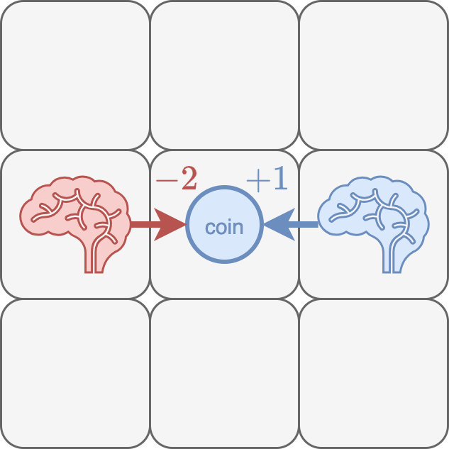
(a) Diagram of CoinGame-2 environment.

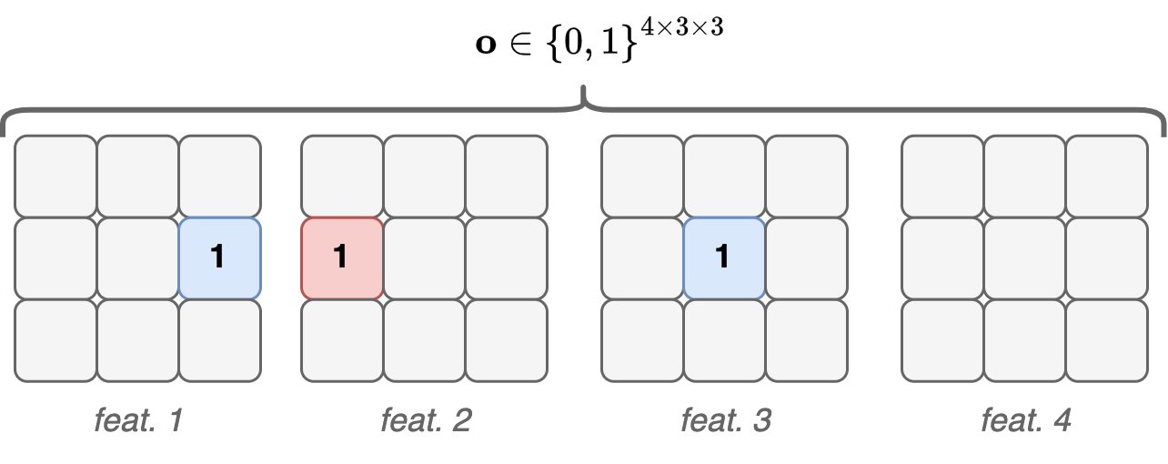
(b) MDP observation dynamics for blue player.

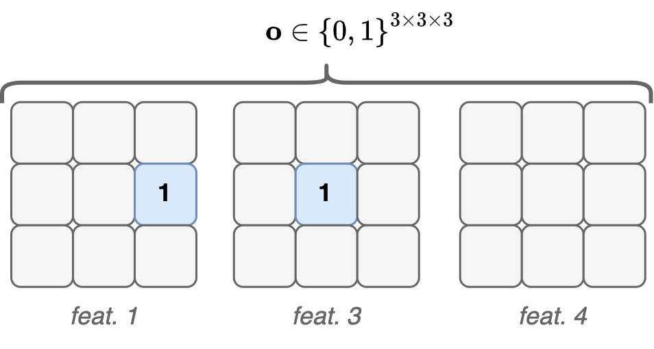
(c) POMDP observation dynamics for blue player.

Figure 4: Example of (a) CoinGame-2 environment with two players, colored red and blue, and a single coin colored blue, with visualization of observation matrix for the blue player with (b) MDP dynamics, and (c) POMDP dynamics. Grid squares in (b) and (c) colored grey denote a $0$ value, and colored blue/red squares denote a $1$ value.

We use the CoinGame environment first proposed in [22], and as implemented in [23], which has been widely used [24, 23, 13] as a benchmark for MARL scenarios. In particular, its nature as a zero-sum game provides an intriguing case study for learning cooperative strategies using full, i.e., described by a MDP, and partial, i.e., described by a POMDP, information. The CoinGame-2 environment pits two agents of different colors (red and blue) on a $3\times 3$ tile grid to collect coins with corresponding color. An example of CoinGame-2 is shown in Fig. 4(a). Agent observations are a sparse matrix $\mathbf{o}\in\{0,1\}^{4\times 3\times 3}$ with 4 features each with a $3\times 3$ grid world as shown in Fig. 4(b). The features specifically are: 1) A grid with a $1$ indicating the agent’s location, 2) A grid with a $1$ to indicate other agent locations, 3) A grid with a $1$ for the location of coins that match the current agent’s color, and 4) A grid with a $1$ for all other coins (different colors). Since these observations include all information about the game world, the game is considered fully observable and is described by an MDP. We also experiment with a partially observable variant of this game which removes the second feature from agent observations (i.e., the location of other agents), which is a space matrix $\mathbf{o}\in\{0,1\}^{3\times 3\times 3}$. In this partially observed setting, the game is described by a POMDP since agents cannot see each other and thus the full state of the game board is unknown. An example of this observation space is shown in Fig. 4(c). The agents can move along the grid by taking actions in the space $\mathcal{A}^{(n)}=\{\textrm{north},\textrm{south},\textrm{east},\textrm{west}\}$ $\forall n\in\mathcal{N}$. Each time an agent collects a coin of their corresponding color their episode reward is increased by $+1$, whereas a different color reduces their episode reward by $-2$. The goal for all agents is to maximize their discounted episode reward. The details of the environment are summarized in Table 1.

We evaluate agents using three metrics: score, total coins collected, and own coin rate. Score, $S=\sum_{n=1}^{N}\sum_{t=0}^{T-1}r^{(n)}_{t}$, aggregates all agent undiscounted rewards over a single episode, where $n\in\mathcal{N}$ is the agent index, $t\in[0,T-1]$ is the episode time index, $T$ is the episode time limit, and $r^{(n)}_{t}$ is the undiscounted agent reward at time $t$. Total coins collected, $TC=\sum_{n=1}^{N}\sum_{t=0}^{T-1}c^{(n)}_{t}$, gives insight into how active the agents were during the game, where $c^{(n)}_{t}$ is the total number of coins collected by agent $n$ at time $t$. Finally, own coin rate, $OCR=\sum_{n=1}^{N}\sum_{t=0}^{T-1}{k^{(n)}_{t}}/{c^{(n)}_{t}}$, gives insight into how the agents achieve cooperation, specifically by being selective on which coins they procure, where $k^{(n)}_{t}$ is the number of coins collected of the corresponding agent’s color.

Table 1: Specifications for CoinGame-2 environment with MDP and POMDP dynamics.

Parameter	Value
Observation for agent $n$ at time $t$	•  MDP:  $\bm{o}^{(n)}_{t}\in\{0,1\}^{4\times 3\times 3}$ (dimension is $36$)
	•  POMDP:  $\bm{o}^{(n)}_{t}\in\{0,1\}^{3\times 3\times 3}$ (dimension is $27$)
Number of players ($N$)	2
Time limit ($T$)	50
Action for agent $n$ at time $t$	$a^{(n)}_{t}\in\{\textrm{north},\textrm{south},\textrm{east},\textrm{west}\}$
Reward for agent $n$ at time $t$	$r^{(n)}_{t}=\begin{cases}+1,&\textrm{if agent $n$ collects coin of same color},\\ -2,&\textrm{if agent $n$ collects coin of different color},\\ 0,&\textrm{otherwise}\end{cases}$
Discount factor ($\gamma$)	0.99
Entropy coefficient ($\alpha$)	0.001

4.2 Quantum encoding transformations

To encode environment observations into our quantum models we first apply a transformation on the observation matrix. This allows us to reduce its dimensions, thereby making it usable for the limited number of qubits available to NISQ systems, while also changing the range of matrix values to be suitable for input into one of the Pauli rotation gates. For the CoinGame-2 environment with fully observed state dynamics we use the transformation $f_{\textrm{MDP}}(\mathbf{o}_{i\times j\times k})=\sum_{k}\mathbf{o}_{i\times j,k}2^{-k}$, which sums over the last dimension of the observation matrix $\mathbf{o}_{i\times j\times k}$ with shape $i\times j\times k$. In the case of CoinGame-2 with MDP dynamics the observations have shape $4\times 3\times 3$. This transformation reduces the dimensions to $4\times 3\times 1$, which can be directly fed into the encoder architecture outlined in Section 3.2. For the CoinGame-2 environment with partially observed state dynamics we use the transformation $f_{\textrm{POMDP}}(\mathbf{o}_{i\times j\times k})=\mathbf{w}\cdot\textrm{flatten}(\mathbf{o}_{i\times j\times k})^{T}+b$, which flattens the observation matrix $\mathbf{o}_{i\times j\times k}$ with shape $i\times j\times k$ and passes it through a single fully-connected NN layer, as done in [11], with parameters $\mathbf{w}_{ijk\times 3d}$ and $b$ and $d$ is the number of qubits. Note that, in POMDP, the trainable quantum encoding parameters $\bm{\lambda}^{(n)}$ are no longer necessary. In this case, we set $\bm{\lambda}^{(n)}=\bm{1}$, where $\bm{1}$ is a matrix of ones.

4.3 Experiment setup

We compare eQMARL against three baselines that considered the current state-of-the-art configurations in actor-critic CTDE: 1) Fully centralized CTDE (fCTDE), a purely classical configuration where the critic is a simple fully-connected NN located at a central server, like in [25, 26], and requires agents to transmit their local observations to the central server via a classical channel; 2) Split CTDE (sCTDE), is another purely classical configuration where the critic is a branching classical NN encoder spread across the agents, and the central server contains a classical NN based on [27]; and 3) Quantum fully centralized CTDE (qfCTDE), a quantum variant of fCTDE where the critic is located at a central server, as in [8, 9, 12], and requires agents to transmit their local observations via a classical channel. These baselines were specifically chosen to convey how a quantum entangled split critic eliminates the transfer of local environment observations, while reducing classical communication overhead by leveraging the quantum channel, and minimizing centralized computational complexity. In our experiments we simplify the setup by using policy sharing across the agents, as done in [9] and [11]. All classical models were built using tensorflow, the quantum models using tensorflow-quantum, and cirq for quantum simulations. All models were trained for 3000 epochs, with $T=50$ steps, $\gamma=0.99$, and the Adam optimizer with varying learning rates. The quantum models use $D=4$ qubits, $L=5$ layers, and $\phi=\texttt{arctan}$ activation. We conduct all experiments on a high-performance computing cluster with 128 AMD CPU cores and 256 GB of memory per node. The training time of eQMARL for MDP is $\approx 3.5~{}\textrm{hours}$, and for POMDP is $\approx 8.5~{}\textrm{hours}$ (see Appendices A, B, and C for hyperparameters, model sizes, and full experiment results).

4.4 Experiment results

4.4.1 Comparing quantum input entanglement styles

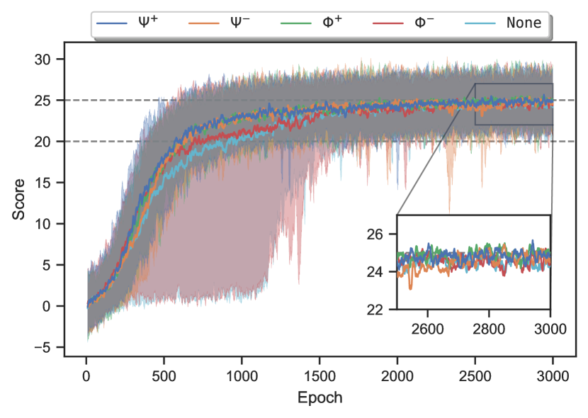
(a) Score - MDP

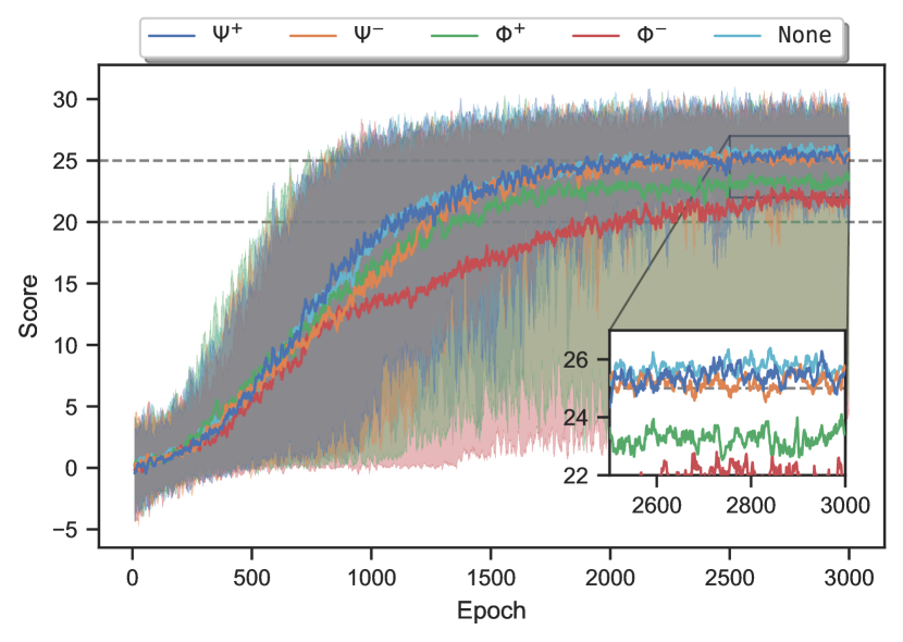
(b) Score - POMDP

Figure 5: Comparison of CoinGame-2 score performance with (a) MDP, and (b) POMDP dynamics for eQMARL using $\Psi^{+}$ (blue), $\Psi^{-}$ (orange), $\Phi^{+}$ (green), $\Phi^{-}$ (red), and None (cyan) entanglement averaged over 10 runs, with min/max ranges shown as shaded regions of corresponding color.

The first set of experiments demonstrate the effectiveness of various input entanglement styles used for our eQMARL approach. We run two separate experiments using the CoinGame-2 environment with both full and partial information. The score metric results for both dynamics are shown in Fig. 5. We specifically consider score thresholds of 20 and 25 which serve as markers to aid our discussion. In the MDP setting of Fig. 5(a), we can see see that $\Psi^{+}$ entanglement achieves a score value of 20 at epoch 568, which is $4.5\%$ faster than $\Psi^{-}$. Similarly, a score of 25 is achieved by $\Phi^{+}$ at epoch 1883, which is $5.2\%$ faster than $\Psi^{-}$. At the end of training, all peak scores hover slightly above 25. Looking at the min/max regions, we get a sense for the stability of each entanglement style. Specifically, we see that $\Psi^{+}$, $\Psi^{-}$, and $\Phi^{+}$ have similar tight ranges until epoch 1500, whereas both $\Phi^{-}$ and None have far lower minimum values until around epoch 1300. Moreover, $\Psi^{-}$ appears to have large downward spikes toward the end of training. Fig. 5(a) shows that there is a gap in convergence between $\Phi^{-}$ and None, and the other styles. Looking closer, we observe that $\Phi^{+}$ plateaus at earlier epochs, and $\Psi^{-}$ is more unstable (dropping in score) at later epochs. Hence, we see a clear advantage for applying $\Psi^{+}$.

In the POMDP setting of Fig. 5(b), we see that $\Psi^{+}$ achieves a score of 20 at epoch 1049, which is about $2\%$ faster than $\mathtt{None}$. Interestingly, there is a much larger gap in convergence between $\Phi^{-}$ and the others. A score of 25 is achieved by $\Psi^{+}$ at epoch 1745, a $10.7\%$ increase over $\mathtt{None}$, whereas both $\Phi^{+}$ and $\Phi^{-}$ never reach this threshold. The final peak scores for $\Psi^{+}$ and $\mathtt{None}$ hover slightly above 26. The min/max regions exhibit a cascade effect between the styles, and, in particular, we observe that $\Phi^{-}$ has the lowest min, followed by $\Phi^{+}$ which has a slightly higher floor. These groupings are interesting as both $\Phi^{+}$ and $\Phi^{-}$ are similar in composition, only differing by a phase. Hence, we again see a clear convergence and score advantage for using $\Psi^{+}$.

Comparing the performance of the entanglement styles with both dynamics paints a picture of the generalizability of the system as a whole. Interestingly, the worse performance of $\Phi^{+}$ and $\Phi^{-}$ suggests that same-state entanglement, $\ket{00}$ and $\ket{11}$, regardless of phase, results in less coupling of agents compared to opposite-state entanglement, $\ket{01}$ and $\ket{10}$. The consistently high performance of $\Psi^{+}$ in both dynamics suggests that it enhances the generalizability of the system, and, since input entanglement does not increase classical computational overhead, we see that $\Psi^{+}$ entanglement can be used to couple the agents in both dynamics while achieving comparable or higher performance. Thus, we select $\Psi^{+}$ as the entanglement scheme to be used in all subsequent experiments.

4.4.2 Comparing baselines with MDP dynamics

(a) Score - MDP

(b) Score - POMDP

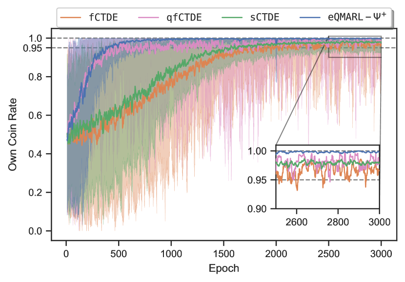
(c) Own coin rate - MDP

(d) Own coin rate - POMDP

Figure 6: Comparison of CoinGame-2 MDP and POMDP environment (a,b) score, and (c,d) own coin rate performance for fCTDE (orange), qfCTDE (magenta), sCTDE (green), and eQMARL-$\Psi^{+}$ (blue) averaged over 10 runs, with min/max ranges shown as shaded regions of corresponding color.

We next compare the performance of eQMARL with the baselines fCTDE, sCTDE, and qfCTDE using the CoinGame-2 environment with MDP state dynamics, as shown in Figs. 6(a) and 6(c). Initially inspecting both score (Fig. 6(a)) and own coin rate (Fig. 6(c)) metrics, we can readily see that eQMARL-$\Psi^{+}$ achieves higher performance with short convergence time. Looking at the score metric in Fig. 6(a), we see that eQMARL-$\Psi^{+}$ achieves a score of 20 at epoch 568, and it converges $16.2\%$ faster than the next closest qfCTDE. A score threshold of 25 is reached by eQMARL-$\Psi^{+}$ at epoch 2332, and it clearly converges $10.8\%$ faster than sCTDE. Overall, we observe a $1.4\%$ increase in max score for eQMARL-$\Psi^{+}$ compared to the next highest sCTDE. Additionally, eQMARL-$\Psi^{+}$ is smoother than qfCTDE at later epochs; suggesting that input entanglement stabilizes convergence.

Fig. 6(c) shows the score in terms of own coin rate, which demonstrates how a cooperative strategy is achieved. We use thresholds of $0.95$ and $1.0$ as markers to gauge performance. From Fig. 6(c), we observe that eQMARL-$\Psi^{+}$ rapidly achieves a $0.95$ rate at epoch 376, and converges to a rate of $1.0$ at epoch 2136. In other words, nearly all the coins each agent collected in the games were of their corresponding color. In contrast, sCTDE, fCTDE, and qfCTDE converge at a much slower pace, never achieve a rate of $1.0$, and exhibit greater fluctuation at the end of the training. From this, we observe that eQMARL-$\Psi^{+}$ converges to a $0.95$ rate $5.3\%$ faster than qfCTDE, and is the only one to achieve a $1.0$ rate. Additionally, we also see that the eQMARL-$\Psi^{+}$ rate curve is smoother than all of the other approaches at later epochs, similar to the score metric.

From Figs. 6(a) and 6(c), we conclude that our proposed eQMARL-$\Psi^{+}$ configuration learns to play the game significantly faster than the classical variants without sharing local observations, transmitting intermediate activations, nor tuning large NNs at the central server. The higher performance and shorter convergence time compared to qfCTDE and both classical fCTDE and sCTDE approaches shows that splitting the critic amongst the agents results in no apparent loss in capability. In fact, the smoothness of the curves suggests that the input entanglement stabilizes the network over time. Further, the own coin rate performance shows that eQMARL-$\Psi^{+}$ learns a cooperative strategy significantly faster than the classical approaches, and with less fluctuation than qfCTDE.

4.4.3 Comparing baselines with POMDP dynamics

Figs. 6(b) and 6(d) show the results of the CoinGame-2 environment with POMDP state dynamics. Fig. 6(b) shows that eQMARL-$\Psi^{+}$ achieves a score value of 20 at epoch 1049, which clearly converges $24\%$ faster considering the noticeable gap between it and qfCTDE. This demonstrates that the branching quantum network with input entanglement shortens convergence time compared to the fully centralized variant Fig. 6(b) also shows that all models achieve a score of 25, however, in this case, eQMARL-$\Psi^{+}$ converges $17.8\%$ faster and with slightly higher score than qfCTDE. Examining smoothness, we see much greater fluctuation between all curves compared to the MDP case.

Fig. 6(d) shows that eQMARL-$\Psi^{+}$ achieves a $0.95$ rate rapidly at epoch 773, converging $25.5\%$ faster than qfCTDE as the next closest. Notice how qfCTDE specifically exhibits greater fluctuation until the $0.95$ rate is achieved. This again suggests that the addition of input entanglement and splitting the quantum critic contribute to smoother convergence. The convergence near threshold $1.0$ paints an interesting picture. We see that qfCTDE actually achieves a perfect $1.0$ rate at epoch 2887, whereas eQMARL-$\Psi^{+}$, sCTDE, and fCTDE never reach this rate; with the highest max value being $0.9996$ for eQMARL-$\Psi^{+}$ at epoch 2533. This is interesting because, despite qfCTDE achieving a higher rate, eQMARL-$\Psi^{+}$ converges to nearly the same rate $12.3\%$ faster. This demonstrates the convergence advantages of incorporating input entanglement into the quantum models while simultaneously splitting the critic amongst the agents over a quantum channel.

The difference in performance between the baselines in Figs. 6(b) and 6(d) demonstrates a clear quantum advantage for learning in the presence of partial information. Specifically, the faster convergence to peak score and own coin rate thresholds in eQMARL-$\Psi^{+}$ demonstrates that splitting the quantum critic across the quantum channel with entangled input qubits allows the agents to learn a more cooperative strategy without direct access to local observations. This is interesting because qfCTDE is centralized and has all local observations at its disposal. This additional information would initially suggest better performance compared to approaches with only local information. However, from Figs. 6(b) and 6(d), we observe a clear benefit for not only splitting the quantum critic as branches across the agents, but also introducing an entangled input state that couples their encoding behavior.

4.4.4 Comparing model sizes

Table 2: Comparison of critic model size in number of trainable parameters for each training framework used on CoinGame-2 environment with MDP and POMDP dynamics.

	Number of Trainable Critic Parameters
Framework	MDP dynamics	POMDP dynamics
eQMARL	265 (132 per agent, 1 central)	817 (408 per agent, 1 central)
qfCTDE	265	817
fCTDE	889	673
sCTDE	913 (444 per agent, 25 central)	697 (336 per agent, 25 central)

Table 2 compares the critic model sizes used in each framework (see Appendix B, Table B.1 for all models). The sizes reported for the critics are for the entire system. This distinction is important since both eQMARL and sCTDE split the critic network across the agents the total size of the agent-specific network is a fraction of the total size. For MDP dynamics, we observe that the quantum models are smaller than the classical variants by about a factor of $4$. For POMDP, we observe that the quantum models are slightly larger overall than their classical counterparts. This is because, in POMDP, the quantum models require a classical NN for dimensionality reduction at the input of each encoder. While the overall system size is larger, however, the number of central parameters is significantly reduced in the quantum cases – requiring only 1 parameter instead of 25. This is important for scaleability because the classical cases implement a full NN at the central server and its size scales with $N$. In contrast, the quantum network only has a single trainable parameter tied to the measurement observable, which will remain fixed regardless of $N$.

5 Conclusion

In this paper, we have proposed eQMARL, a novel quantum actor-critic framework for training decentralized policies using a split quantum critic with entangled input qubits and joint measurement. Spreading the critic across the agents via a quantum channel eliminates sharing local observations, minimizes the classical communication overhead from sending model parameters or intermediate NN activations, and reduces the centralized classical computational burden through optimization of a single quantum measurement observable parameter. We have shown that $\Psi^{+}$ input entanglement improves agent cooperation and system generalizability across both MDP and POMDP environments. For MDP, we have shown that eQMARL converges to a cooperative strategy $10.8\%$ faster and with a higher score compared to sCTDE. Likewise, for POMDP, we have shown that eQMARL converges to a cooperative strategy $17.8\%$ faster and with slightly higher score compared to qfCTDE. Further, we have shown that eQMARL requires $25$-times fewer centralized parameters compared to sCTDE. From a broader impact perspective, there is indeed a potential synergy between eQMARL and multi-agent system security. Agent privacy could be bolstered from the elimination of local observation sharing, and environmental eavesdropping could be monitored via detecting measurement anomalies over the quantum channel (similar to quantum key distribution). Future works could investigate the potential privacy and security benefits of eQMARL, such as these, for impacts to safeguarding multi-agent system confidentiality and integrity.

Appendix A Model hyperparameters

The hyperparameters for each of the models trained in our experiments, as discussed in Section 4.3, are shown in Tables A.1 and A.2. Table A.1 shows the parameters for the quantum models, as used in qfCTDE and eQMARL. Table A.2 shows the paramters for the classical models, as used in fCTDE and sCTDE.

Table A.1: Hyperparameters for both qfCTDE and eQMARL, actor and critic, used on CoinGame-2 environment with MDP and POMDP dynamics.

Parameter	Value
NN encoder transform activation	•  MDP:  N/A
	•  POMDP:  linear
Flag $\bm{\lambda}^{(n)}$ as trainable	•  MDP:  True
	•  POMDP:  False
Number of qubits per agent ($D$)	4
(eQMARL only) Input entanglement type ($B$) for critic	$\Psi^{+}$
Number of layers ($L$) in $U_{\textrm{vqc}}$	5
Squash activation ($\phi$)	arctan
Inverse temperature ($\beta$)	1
Optimizer	Adam
Learning rate	$[0.01,0.1,0.1]$

Table A.2: Hyperparameters for both fCTDE and sCTDE, actor and critic, used on CoinGame-2 environment with MDP and POMDP dynamics.

Parameter	Value
NN hidden units	$[12]$
Activation	ReLU
Optimizer	Adam
Learning rate	$0.001$

Appendix B Model sizes

The sizes of the actor and critic models, in number of trainable parameters, for eQMARL, qfCTDE, fCTDE, and sCTDE as discussed in Section 4.4.4 are shown in Table B.1.

Table B.1: Comparison of model size in number of trainable parameters for each training framework used on CoinGame-2 environment with MDP and POMDP dynamics.

		Number of Trainable Parameters
Framework	Model	MDP dynamics	POMDP dynamics
eQMARL	Actor	136	412
	Critic	265 (132 per agent, 1 central)	817 (408 per agent, 1 central)
qfCTDE	Actor	136	412
	Critic	265	817
fCTDE	Actor	496	388
	Critic	889	673
sCTDE	Actor	496	388
	Critic	913 (444 per agent, 25 central)	697 (336 per agent, 25 central)

Appendix C Experiment results

The empirical results for eQMARL, qfCTDE, fCTDE, and sCTDE, as discussed in Section 4.4, are shown in Tables C.1, C.2, C.1, and C.2. Table C.1 shows the convergence time, in epochs, to each of the score thresholds 20, 25, and also to the maximum score value (reported parenthetically in italics) for each of the entanglement styles $\Psi^{+}$, $\Psi^{-}$, $\Phi^{+}$, $\Phi^{-}$, and $\mathtt{None}$, as discussed in Section 4.4.1. Table C.1 shows the convergence time to each of the score thresholds, in addition to the own coin rate thresholds, for eQMARL-$\Psi^{+}$, qfCTDE, sCTDE, and fCTDE, as discussed in Sections 4.4.2 and 4.4.3. The best values in each column are highlighted in bold.

Table C.1: Comparison of entanglement style score convergence (in number of epochs) for MDP and POMDP CoinGame-2 environment dynamics. Best values are highlighted in bold.

		Epochs to Score Threshold
Dynamics	Entanglement	20	25	Max (value)
MDP	$\Psi^{+}$	568	2332	2942 (25.67)
	$\Psi^{-}$	595	1987	2849 (25.45)
	$\Phi^{+}$	612	1883	2851 (25.51)
	$\Phi^{-}$	691	2378	2984 (25.23)
	$\mathtt{None}$	839	2337	2495 (25.12)
POMDP	$\Psi^{+}$	1049	1745	2950 (26.28)
	$\Psi^{-}$	1206	2114	2999 (25.95)
	$\Phi^{+}$	1269	-	2992 (24.1)
	$\Phi^{-}$	1838	-	2727 (22.8)
	$\mathtt{None}$	1069	1955	2841 (26.39)

Table C.2: Comparison of model score and own coin rate convergence (in number of epochs) for MDP and POMDP CoinGame-2 environment dynamics. Best values are highlighted in bold.

		Epochs to Score Threshold			Epochs to Own Coin Rate Threshold
Dynamics	Framework	20	25	Max (value)	0.95	1.0	Max (value)
MDP	eQMARL-$\Psi^{+}$	568	2332	2942 (25.67)	376	2136	2136 (1.0)
	qfCTDE	678	-	2378 (23.38)	397	-	2832 (0.9972)
	sCTDE	1640	2615	2631 (25.3)	1511	-	2637 (0.9864)
	fCTDE	1917	-	2925 (23.67)	1700	-	2909 (0.9857)
POMDP	eQMARL-$\Psi^{+}$	1049	1745	2950 (26.28)	773	-	2533 (0.9997)
	qfCTDE	1382	2124	2871 (26.09)	1038	2887	2887 (1.0)
	sCTDE	1738	2750	2999 (25.33)	1588	-	2956 (0.9894)
	fCTDE	1798	2658	2824 (25.49)	1574	-	2963 (0.9894)

Figs. C.1 and C.2 show the training results for the entanglement styles, and various frameworks as discussed in Sections 4.4.1, 4.4.2, and 4.4.3. In particular, we provide the full set of performance metrics of score, total coins collected, own coins collected, and own coin rate, as outlined in Section 4.1. Fig. C.1 shows the results for the entanglement styles $\Psi^{+}$, $\Psi^{-}$, $\Phi^{+}$, $\Phi^{-}$, and $\mathtt{None}$, as discussed in Section 4.4.1. The left column, Figs. 1(a), 1(c), 1(e), and 1(g), shows the performance for MDP environment dynamics. Similarly, the right column, Figs. 1(b), 1(d), 1(f), and 1(h), shows the performance for POMDP environment dynamics. Fig. C.2 shows the results for eQMARL-$\Psi^{+}$, qfCTDE, sCTDE, and fCTDE, as discussed in Sections 4.4.2 and 4.4.3. The performance for MDP dynamics is shown in Figs. 2(a), 2(c), 2(e), and 2(g), and for POMDP dynamics is shown in Figs. 2(b), 2(d), 2(f), and 2(h). Importantly, Figs. C.1 and C.2 shed light on when, and how, a cooperative strategy is achieved by each framework. Further, through Figs. C.1 and C.2 we also observe the relationship between the metrics outlined in Section 4.1. This connection is important, as a single metric in isolation only paints part of the performance picture. A full comparison can be achieved by considering the metrics as as group, and, particularly, the relationship between agent score, i.e., the sum of rewards, and own coin rate, i.e., the priority given to coins of matching color.

(a) Score - MDP

(b) Score - POMDP

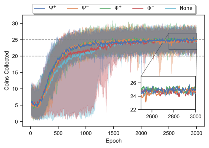
(c) Total coins collected - MDP

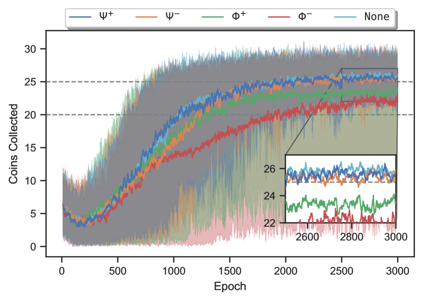
(d) Total coins collected - POMDP

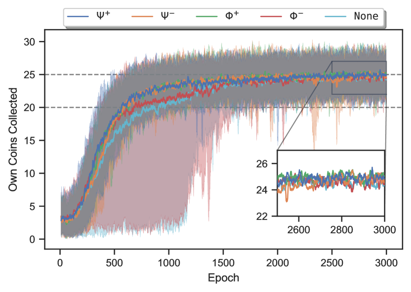
(e) Own coins collected - MDP

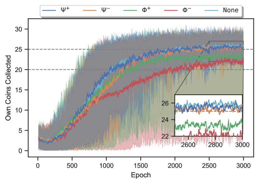
(f) Own coins collected - POMDP

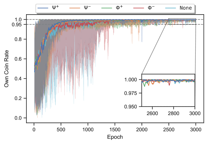
(g) Own coin rate - MDP

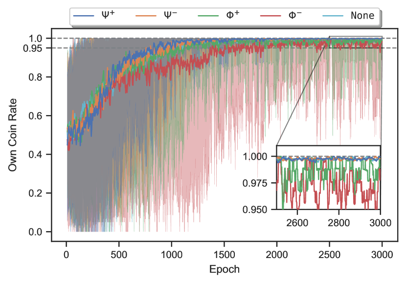
(h) Own coin rate - POMDP

Figure C.1: Comparison of CoinGame-2 MDP and POMDP environment performance metrics (a,b) score, (c,d) total coins collected, (e,f) own coins collected, and (g,h) own coin rate for eQMARL with varying input quantum entanglement styles $\Psi^{+}$ (blue), $\Psi^{-}$ (orange), $\Phi^{+}$ (green), $\Phi^{-}$ (red), and None (cyan) averaged over 10 runs, with min/max ranges shown as shaded regions of corresponding color.

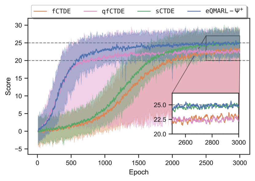
(a) Score - MDP

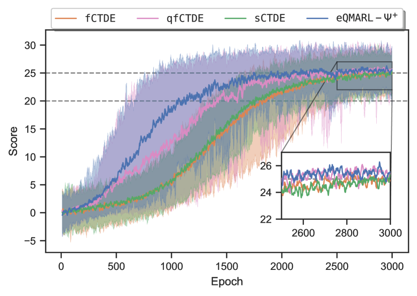
(b) Score - POMDP

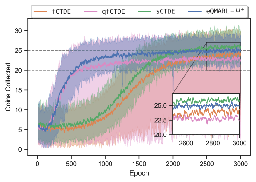
(c) Total coins collected - MDP

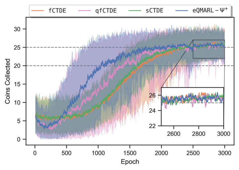
(d) Total coins collected - POMDP

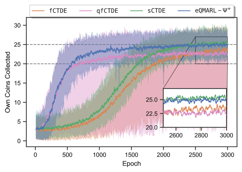
(e) Own coins collected - MDP

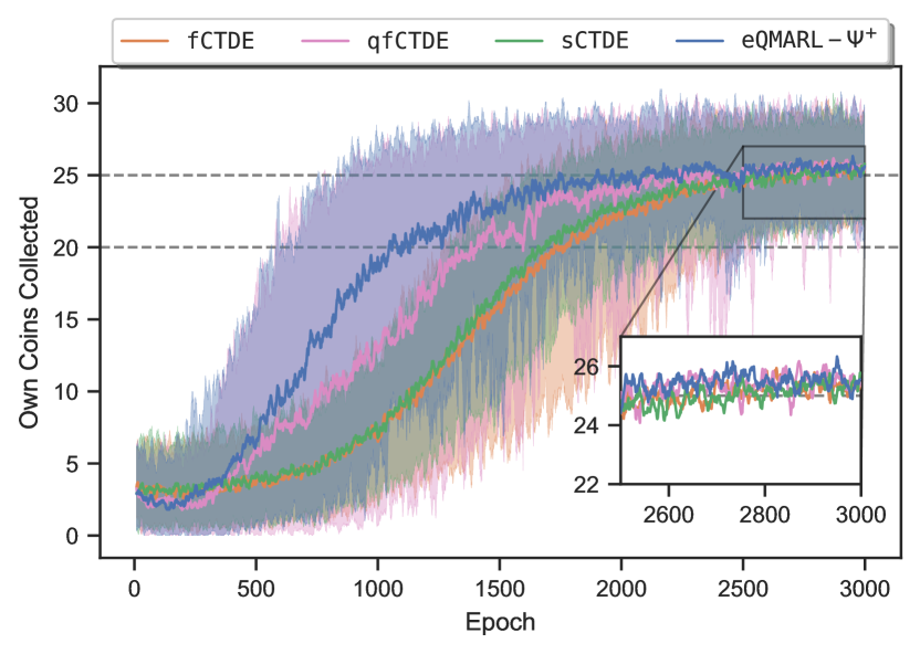
(f) Own coins collected - POMDP

(g) Own coin rate - MDP

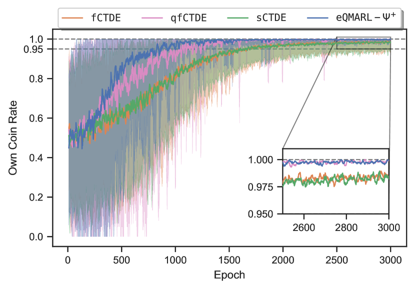
(h) Own coin rate - POMDP

Figure C.2: Comparison of CoinGame-2 MDP and POMDP environment performance metrics (a,b) score, (c,d) total coins collected, (e,f) own coins collected, and (g,h) own coin rate for fCTDE (orange), qfCTDE (magenta), sCTDE (green), and eQMARL-$\Psi^{+}$ (blue) averaged over 10 runs, with min/max ranges shown as shaded regions of corresponding color.

References

- [1] Dylan Herman et al. “A Survey of Quantum Computing for Finance” arXiv, 2022 arXiv: http://arxiv.org/abs/2201.02773
- [2] Frederik F. Flöther “The State of Quantum Computing Applications in Health and Medicine” In Research Directions: Quantum Technologies, 2023, pp. 1–21 DOI: 10.1017/qut.2023.4
- [3] Bhaskara Narottama, Zina Mohamed and Sonia Aïssa “Quantum Machine Learning for Next-G Wireless Communications: Fundamentals and the Path Ahead” In IEEE Open Journal of the Communications Society 4, 2023, pp. 2204–2224 DOI: 10.1109/OJCOMS.2023.3309268
- [4] A. Einstein, M. Born and H. Born “The Born-Einstein Letters: Correspondence between Albert Einstein and Max and Hedwig Born from 1916-1955, with Commentaries by Max Born” Macmillan, 1971 URL: https://books.google.com/books?id=HvZAAQAAIAAJ
- [5] Kosuke Mitarai, Makoto Negoro, Masahiro Kitagawa and Keisuke Fujii “Quantum Circuit Learning” In Physical Review A 98.3, 2018, pp. 032309 DOI: 10.1103/PhysRevA.98.032309
- [6] Yuxuan Du, Min-Hsiu Hsieh, Tongliang Liu and Dacheng Tao “The Expressive Power of Parameterized Quantum Circuits” In Physical Review Research 2.3, 2020, pp. 033125 DOI: 10.1103/PhysRevResearch.2.033125
- [7] Won Joon Yun, Hankyul Baek and Joongheon Kim “Quantum Split Neural Network Learning Using Cross-Channel Pooling” arXiv, 2023 arXiv: http://arxiv.org/abs/2211.06524
- [8] Won Joon Yun et al. “Quantum Multi-Agent Reinforcement Learning via Variational Quantum Circuit Design” arXiv, 2022 DOI: 10.48550/arXiv.2203.10443
- [9] Won Joon Yun et al. “Quantum Multi-Agent Actor-Critic Neural Networks for Internet-Connected Multi-Robot Coordination in Smart Factory Management”, 2023 DOI: 10.48550/arXiv.2301.04012
- [10] Won Joon Yun, Jihong Park and Joongheon Kim “Quantum Multi-Agent Meta Reinforcement Learning”, 2022 arXiv: http://arxiv.org/abs/2208.11510
- [11] Samuel Yen-Chi Chen “Asynchronous Training of Quantum Reinforcement Learning” arXiv, 2023 DOI: 10.48550/arXiv.2301.05096
- [12] Soohyun Park et al. “Quantum Multi-Agent Reinforcement Learning for Autonomous Mobility Cooperation” arXiv, 2023 arXiv: http://arxiv.org/abs/2308.01519
- [13] Michael Kölle et al. “Multi-Agent Quantum Reinforcement Learning Using Evolutionary Optimization” arXiv, 2024 arXiv: http://arxiv.org/abs/2311.05546
- [14] Max Born “Quantenmechanik Der Stoßvorgänge” In Zeitschrift für Physik 38.11, 1926, pp. 803–827
- [15] Fabrizio Logiurato and Augusto Smerzi “Born Rule and Noncontextual Probability” In Journal of Modern Physics 03.11, 2012, pp. 1802–1812 DOI: 10.4236/jmp.2012.311225
- [16] Lluís Masanes, Thomas D. Galley and Markus P. Müller “The Measurement Postulates of Quantum Mechanics Are Operationally Redundant” In Nature Communications 10.1 Springer Science and Business Media LLC, 2019 DOI: 10.1038/s41467-019-09348-x
- [17] Michael A. Nielsen and Isaac L. Chuang “Quantum Computation and Quantum Information: 10th Anniversary Edition” Cambridge University Press, 2012 DOI: 10.1017/CBO9780511976667
- [18] Praneeth Vepakomma, Otkrist Gupta, Tristan Swedish and Ramesh Raskar “Split Learning for Health: Distributed Deep Learning without Sharing Raw Patient Data”, 2018 arXiv: http://arxiv.org/abs/1812.00564
- [19] Sofiene Jerbi et al. “Parametrized Quantum Policies for Reinforcement Learning”, 2021 DOI: 10.48550/arXiv.2103.05577
- [20] Andrea Skolik, Sofiene Jerbi and Vedran Dunjko “Quantum Agents in the Gym: A Variational Quantum Algorithm for Deep Q-learning”, 2021 DOI: 10.22331/q-2022-05-24-720
- [21] Georgios Papoudakis, Filippos Christianos, Lukas Schäfer and Stefano V. Albrecht “Benchmarking Multi-Agent Deep Reinforcement Learning Algorithms in Cooperative Tasks” arXiv, 2021 arXiv: http://arxiv.org/abs/2006.07869
- [22] Adam Lerer and Alexander Peysakhovich “Maintaining Cooperation in Complex Social Dilemmas Using Deep Reinforcement Learning” arXiv, 2018 arXiv: http://arxiv.org/abs/1707.01068
- [23] Thomy Phan et al. “Emergent Cooperation from Mutual Acknowledgment Exchange” In Proceedings of the 21st International Conference on Autonomous Agents and Multiagent Systems, AAMAS ’22 Richland, SC: International Foundation for Autonomous Agents and Multiagent Systems, 2022, pp. 1047–1055
- [24] Jakob N. Foerster et al. “Learning with Opponent-Learning Awareness” arXiv, 2018 arXiv: http://arxiv.org/abs/1709.04326
- [25] Jayesh K. Gupta, Maxim Egorov and Mykel Kochenderfer “Cooperative Multi-agent Control Using Deep Reinforcement Learning” In Autonomous Agents and Multiagent Systems 10642 Cham: Springer International Publishing, 2017, pp. 66–83 DOI: 10.1007/978-3-319-71682-4_5
- [26] Jakob Foerster et al. “Counterfactual Multi-Agent Policy Gradients” In Proceedings of the AAAI Conference on Artificial Intelligence 32.1, 2018 DOI: 10.1609/aaai.v32i1.11794
- [27] Tabish Rashid et al. “QMIX: Monotonic Value Function Factorisation for Deep Multi-Agent Reinforcement Learning” arXiv, 2018 arXiv: http://arxiv.org/abs/1803.11485