FreezeAsGuard: Mitigating Illegal Adaptation of Diffusion Models via Selective Tensor Freezing

Abstract

Text-to-image diffusion models can be fine-tuned in custom domains to adapt to specific user preferences, but such unconstrained adaptability has also been utilized for illegal purposes, such as forging public figures’ portraits and duplicating copyrighted artworks. Most existing work focuses on detecting the illegally generated contents, but cannot prevent or mitigate illegal adaptations of diffusion models. Other schemes of model unlearning and reinitialization, similarly, cannot prevent users from relearning the knowledge of illegal model adaptation with custom data. In this paper, we present FreezeAsGuard, a new technique that addresses these limitations and enables irreversible mitigation of illegal adaptations of diffusion models. The basic approach is that the model publisher selectively freezes tensors in pre-trained diffusion models that are critical to illegal model adaptations, to mitigate the fine-tuned model’s representation power in illegal domains but minimize the impact on legal model adaptations in other domains. Such tensor freezing can be enforced via APIs provided by the model publisher for fine-tuning, can motivate users’ adoption due to its computational savings. Experiment results with datasets in multiple domains show that FreezeAsGuard provides stronger power in mitigating illegal model adaptations of generating fake public figures’ portraits, while having the minimum impact on model adaptation in other legal domains. The source code is available at: https://github.com/pittisl/FreezeAsGuard.

1 Introduction

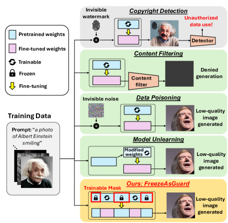
Figure 1: Existing work vs. FreezeAsGuard in mitigating malicious adaptation of diffusion models

Text-to-image diffusion models [43; 42] are powerful tools to generate high-quality images aligned with user prompts. After being pre-trained by model publishers to embed world knowledge from large image data [48], open-sourced diffusion models, such as Stable Diffusion (SD) [8; 9], can be conveniently adapted by users to generate their preferred images, through fine-tuning with custom data in specific domains. For example, diffusion models can be fine-tuned on cartoon datasets to synthesize avatars in video games [45], or on datasets of landscape photos to generate wallpapers [11].

An increasing risk of democratizing open-sourced diffusion models, however, is that the capability of model adaptation has been utilized for illegal purposes, such as forging public figures’ portraits [24; 26], duplicating copyrighted artworks [28], and generating sexual content [27]. Most existing efforts aim to deter attempts of illegal model adaptation with copyright detection [58; 18; 19], which embeds invisible but detectable watermarks into training data and further generated images, as shown in Figure 1. However, such detection only applies to misuse of training data, and does not mitigate the user’s capability of illegal model adaptation.

Instead, an intuitive approach to mitigation is content filtering. However, filtering user prompts [20] can be bypassed by fine-tuning the model to align innocent prompts with illegal image contents [51], and filtering the generated images [6] is often overpowered with high false-positive rates [1]. Data poisoning techniques can avoid false positives by injecting invisible perturbations into training data [54; 57; 49], but cannot apply when public data or users’ private data is used for fine-tuning. Recent unlearning methods allow model publishers to remove knowledge needed for illegal adaptation by modifying model weights [21; 25; 53; 59] , but cannot prevent relearning such knowledge via fine-tuning.

The key limitation of the aforementioned existing techniques is that they focus on modifying the training data or model weights, but such modification can be easily reversed by users via fine-tuning with their custom data. Such modification, furthermore, cannot precisely focus the mitigation power only in illegal domains without affecting model adaptation in other innocent domains, due to the high ambiguity when fine-tuning diffusion models in different domains.

To prevent users from reversing the mitigation maneuvers being applied on diffusion models, in this paper we present a new technique, namely FreezeAsGuard, which advocates a fundamental shift that constrains the trainability of diffusion model’s tensors in fine-tuning. As shown in Figure 1, the model publisher selectively freezes tensors in pre-trained models that are critical to the convergence of fine-tuning in illegal domains, to limit the model’s representation power of being fine-tuned in illegal domains. In practice, since most users fine-tune diffusion models by following instructions and using APIs provided by model publishers, tensor freezing can be effectively enforced by model publishers through these APIs. Meanwhile, since freezing tensors significantly reduces the computational costs of fine-tuning, users are well motivated to adopt tensor freezing in fine-tuning practices.

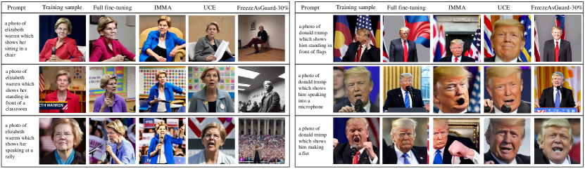
Figure 2: FreezeAsGuard ensures that portrait images generated by fine-tuned model in illegal domains cannot be recognizable as target subjects. In contrast, unlearning schemes (UCE [25] and IMMA [59]) cannot prevent the unlearned knowledge of illegal domains from being relearned in fine-tuning.

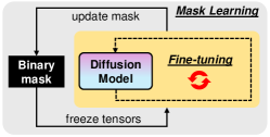
Figure 3: Mask learning and fine-tuning are combined as bilevel optimization

The major challenge is how to properly evaluate the importance of tensors in model fine-tuning. Popular attribution-based importance metrics [37; 40] are mainly used in model pruning with fixed weight values, but cannot reflect the impact of weight variations in fine-tuning. Such impact of weight variations, in fact, cannot be condensed into a single importance metric, due to the randomness and interdependencies of weight updates in fine-tuning iterations. Instead, as shown in Figure 3, we formulate the selection of frozen tensors as a trainable binary mask. Given a required ratio of frozen tensors specified by the model publisher, we optimize such selection with training data samples in illegal domains, through bilevel optimization that combines the iterative process of mask learning and the iterations of model fine-tuning. In this way, we ensure that the mask being trained can timely learn the impact of weight variations on the training loss during fine-tuning.

With frozen tensors, the model’s representation power should be retained when fine-tuned in innocent domains. Hence, we further incorporate training samples from innocent domains into the bilevel optimization, to provide suppressing signals for selecting tensors being frozen. Hence, the learned mask of freezing tensors should skip tensors that are important to fine-tuning in innocent domains.

We evaluated FreezeAsGuard in a challenging mitigation of illegal model adaptation: generating fake portraits of public figures, with open-sourced SD models. We use a self-collected dataset of 25 public figures’ portraits as illegal domain, Modern-Logo-v4 [4] and H&M-Clothes [3] datasets as innocent domain, and competitive model unlearning schemes as baselines. Our main findings are as follows:

• FreezeAsGuard has strong mitigation power in illegal domains. It reduces the quality of images generated by fine-tuned model by 14% compared to baselines, and ensures the generated images to be unrecognizable as target subjects, as shown in Figure 2 and Section 4.2.

• FreezeAsGuard has the minimum impact on legal modal adaptation in innocent domains. It can achieve on-par quality of the generated images with regular full fine-tuning on innocent datasets. Compared to the competitive baselines, it improves the accuracy by up to 8%.

• FreezeAsGuard has high compute efficiency. Compared to baseline schemes, it can save up to 48% GPU memory and 21% wall-clock time of model fine-tuning for innocent users.

2 Background & Motivation

2.1 Fine-tuning Diffusion Models in illegal domains

Given text prompts $y$ and images $x$ as training data, fine-tuning a diffusion model approximates the conditional distribution $p(x|y)$ by learning to reconstruct images that are progressively blurred with Gaussian noise $\epsilon$ over step $t=1,...,T$. The training objective is to minimize the reconstruction loss:

$$\mathcal{L}_{DM}=\mathbb{E}_{x,y,\epsilon\sim\mathcal{N}(0,1),t}\left[\|\epsilon-\epsilon_{\theta}(\mathcal{E}(x_{t}),t,\tau(y))\|^{2}_{2}\right],$$ (1)

where $\mathcal{E}(\cdot)$ is the encoder of a pretrained VAE, $\tau(\cdot)$ is a pretrained text encoder, and $\epsilon_{\theta}(\cdot)$ is a denoising model with trainable parameters $\theta$. Most existing diffusion models adopt the UNet architecture [44] for the denoising model, which is then used to generate images from noise, conditioned by user prompts.

In fine-tuning, the diffusion model learns new knowledge in illegal domains by adopting generic knowledge in the pre-trained model [14]. For example, knowledge about “a green beetle” in illegal domains can be a combination of knowledge on “hornet” and “emerald” in pre-trained model. This behavior implies that fine-tuning in different domains shares the same knowledge base, and it is hence challenging to focus the mitigation power in illegal domains without affecting fine-tuning in innocent domains. This challenge motivates us to regulate FreezeAsGuard’s mitigation power by incorporating training samples in innocent domains, when selecting tensors being frozen for illegal domains.

In most fine-tuning practices, LoRA adapters [32; 46] and prompt tuning [23] are used to reduce memory costs. These methods, however, restrict the number of trainable UNet parameters and reduce the representation power of fine-tuned models in illegal domains. In this paper, we instead consider a more challenging scenario of tensor freezing, where all UNet parameters are trainable in fine-tuning.

Model component Being frozen	CLIP ($\uparrow$)	TOPIQ ($\uparrow$)	FID ($\downarrow$)
No freezing	31.93	0.054	202.18
Attention projectors	31.60	0.051	208.40
Conv. layers	31.54	0.047	206.58
Time embeddings	31.46	0.045	212.79
50% random weights (seed 1)	32.25	0.054	206.53
50% random weights (seed 2)	32.62	0.051	216.12

Table 1: Quality of generated images with different model compoents being frozen when fine-tuning SD v1.5 [8] on the captioned pokemon dataset [5], using CLIP [29, TOPIQ [15], and FID [30] image quality metrics

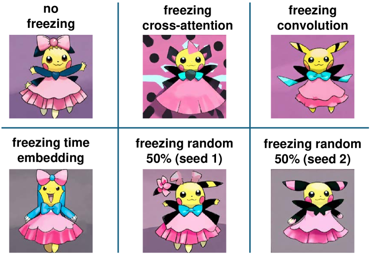
Figure 4: Generated images with different model components being frozen, when using the prompt “a cartoon pikachu with a pink dress and a pink bow”

2.2 Partial Model Fine-tuning

Different model components have specialized functionalities, and hence fine-tuning only some of them results in different model performances. For diffusion models, we cannot mitigate illegal model adaptations in illegal domains by simply excluding some layers from being fine-tuned, because shallow layers provide primary image features and deep layers enforce domain-specific semantics [56]. They are, hence, both essential to the performance of the fine-tuned models in innocent domains.

Similarly, although large diffusion models have modularized structures, it is inappropriate to completely exclude specific model components from being fine-tuned. As shown in Table 1 and Figure 4, freezing critical components such as attention projectors and time embeddings can cause non-negligible quality drop in generated images. Even when freezing the same amount of model weights (e.g., random 50%), the exact distribution of frozen weights could also affect the generated images’ quality. Such heterogeneity motivates us to instead seek for globally optimal selections of freezing tensors across all model components, by jointly taking all model components into bilevel optimization.

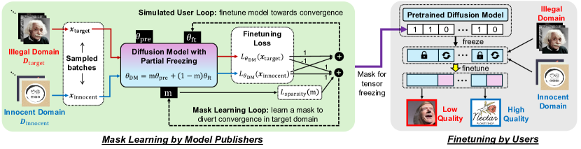
Figure 5: Overview of FreezeAsGuard design

3 Method

Our design of FreezeAsGuard builds on bilevel optimization, which embeds one optimization problem within another [16; 39; 22]. This bilevel optimization can be formulated as

$$\mathbf{m}^{*} =\arg\min_{\mathbf{m}}\left(-\mathcal{L}_{\boldsymbol{\theta}^{*}(\mathbf{m})}(\mathbf{x}_{illegal}),\mathcal{L}_{\boldsymbol{\theta}^{*}(\mathbf{m})}(\mathbf{x}_{innocent})\right)$$ (2)

$$\text{s.t.}\ \ \ \boldsymbol{\theta}^{*}(\mathbf{m})=\arg\min_{\boldsymbol{\theta}(\mathbf{m})}\left(\mathcal{L}_{\boldsymbol{\theta}(\mathbf{m})}(\mathbf{x}_{illegal}),\mathcal{L}_{\boldsymbol{\theta}(\mathbf{m})}(\mathbf{x}_{innocent})\right),\vspace{-0.05in}$$ (3)

where $\mathbf{m}$ is the binary mask of selecting frozen tensors, $\mathbf{m}^{*}$ is the optimized binary mask, $\boldsymbol{\theta}(\mathbf{m})$ represents the model tensors frozen by $\mathbf{m}$, and $\boldsymbol{\theta}^{*}(\mathbf{m})$ is the converged $\boldsymbol{\theta}(\mathbf{m})$ after fine-tuning. $\mathbf{x}_{illegal}$ and $\mathbf{x}_{innocent}$ denote training samples in illegal domains ($\mathcal{D}_{illegal}$) and innocent domains ($\mathcal{D}_{innocent}$), respectively. Such bilevel optimization is illustrated in Figure 5. The lower-level problem in Eq. (3) is a simulated user loop that the user fine-tunes the diffusion model towards convergence by minimizing the loss over both illegal and innocent domains. The upper-level problem in Eq. (2) is a mask learning loop that the model publisher learns $\mathbf{m}$ to mitigate the diffusion model’s representation power when being fine-tuned in illegal domains, without affecting fine-tuning in innocent domains.

Some existing work adopts differentiable image quality metrics (e.g., MS-SSIM [50]) to measure the convergence of fine-tuning, but suffers from gradient explosion during optimization [54]. Instead, in FreezeAsGuard we use the standard diffusion loss in Eq. (1), and adopt tensor-level freezing to ensure sufficient granularity, without incurring extra computing costs.

To apply the gradient solver, $\mathbf{m}$ and $\boldsymbol{\theta}(\mathbf{m})$ should have differentiable dependencies with the loss function calculation. We model $\boldsymbol{\theta}(\mathbf{m})$ through the weighted summation of pre-trained model tensors $\boldsymbol{\theta}_{pre}$ and fine-tuned model tensors $\boldsymbol{\theta}_{ft}$, such that

$$\boldsymbol{\theta}(\mathbf{m})=\mathbf{m}\odot\boldsymbol{\theta}_{pre}+(\mathbf{1}-\mathbf{m})\odot\boldsymbol{\theta}_{ft},\vspace{-0.05in}$$ (4)

where $\odot$ denotes element-wise multiplication. From the user’s perspective, fine-tuning the partially frozen model $\boldsymbol{\theta}(\mathbf{m})$ is equivalent to fine-tuning the $\boldsymbol{\theta}_{ft}$ component. In that case, $\boldsymbol{\theta}_{ft}$ is controlled by the constraint in Eq. (3). To improve compute efficiency, we initialize $\boldsymbol{\theta}_{ft}$ as the fully fine-tuned model tensors in both illegal and innocent domains, and gradually enlarge the scope of tensors being frozen. Besides, since $\mathbf{m}$ is discrete and not differentiable, in practice we adopt a continuous form $\mathbf{m}(\mathbf{w})=\sigma(\mathbf{w}/T)$ that applies sigmoid function $\sigma(\cdot)$ over a trainable tensor $\mathbf{w}$. We also developed code optimizations to allow vectorized gradient calculations, and details can be found in Appendix A.

3.1 Mask Learning in the Upper-level Loop

To solve the upper-level multi-objective optimization in Eq. (2), we adopt linear scalarization [33] to convert it into a single objective $\mathcal{L}_{upper}$ via a weighted summation with weights $(\lambda_{1},\lambda_{2})$:

$$\mathcal{L}_{upper}=-\lambda_{1}\mathcal{L}_{\boldsymbol{\theta}^{*}(\mathbf{m})}(\mathbf{x}_{illegal})+\lambda_{2}\mathcal{L}_{\boldsymbol{\theta}^{*}(\mathbf{m})}(\mathbf{x}_{innocent}),\vspace{-0.05in}$$ (5)

to involve training samples in both illegal and innocent domains when learning $\mathbf{m}$. Intuitively, $(\lambda_{1},\lambda_{2})$ should ensure that gradient-based feedbacks from the two loss terms are not biased by any inequality between the amounts of $\mathbf{x}_{illegal}$ and $\mathbf{x}_{innocent}$. In practice, we can set $(\lambda_{1},\lambda_{2})=(1,1)$ because computing expectation in the diffusion loss in Eq. (1) has normalized the loss to sample-wise magnitude.

Besides, $\mathbf{x}_{illegal}$ and $\mathbf{x}_{innocent}$ could contain some knowledge in common, and masked learning from such data may hence affect model adaptation in innocent domains. To address this problem, we add a sparsity constraint $\mathcal{L}_{sparsity}$ to $\mathcal{L}_{upper}$ to better control of the mask’s mitigation power:

$$\mathcal{L}_{sparsity}=\|\mathbf{1}^{\top}\mathbf{m}/N-\rho\|_{2}^{2},\vspace{-0.05in}$$ (6)

where $N$ is the total number of tensors and $\mathbf{1}^{\top}\mathbf{m}/N$ measures the proportion of tensors being frozen. By minimizing $\mathcal{L}_{sparsity}$, the achieved ratio of tensor freezing should approach the given $\rho$ specified by model publisher. In this way, we can apply gradient descent to minimize $\mathcal{L}_{upper}$ and iteratively refine $\mathbf{m}$ towards optimum, and we will experimentally investigate the optimal value of $\rho$ in Section 4.

3.2 Model Fine-tuning in the Lower-level Loop

Effectiveness of mask learning at the upper level relies on timely feedback from the lower-level fine-tuning. Every time the mask has been updated by an iteration in the upper level, the lower-level loop should adopt the updated mask into fine-tuning, and return the fine-tuned model tensors and the correspondingly updated loss value as feedback to the upper level. Similar to Eq. (5), the fine-tuning objective is the summation of diffusion losses for illegal and innocent domains:

$$\mathcal{L}_{lower}=\mathcal{L}_{\boldsymbol{\theta}^{*}(\mathbf{m})}(\mathbf{x}_{illegal})+\mathcal{L}_{\boldsymbol{\theta}^{*}(\mathbf{m})}(\mathbf{x}_{innocent}).\vspace{-0.05in}$$ (7)

3.3 Improving the Compute Efficiency of Bilevel Optimization

Solving bilevel optimization has known to be computationally expensive, due to the repeated switches between the upper-level and lower-level loops [46; 59]. Rigorously, as shown in Figure 6 - Left, every time when the mask has been updated, the model should be fine-tuned with a sufficient number of iterations until convergence, before the next update of the mask. In this way, the mask can be optimized to maximize the loss value when fine-tuning converges. However, in practice, doing so is extremely expensive, given the possibly large number of mask updates before reaching $\mathbf{m}^{*}$.

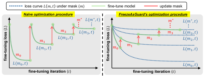
Figure 6: FreezeAsGuard vs. Naive optimization iterations

Instead, as shown in Figure 6 - Right, we observe that the fine-tuning loss typically drops fast in the first few iterations and then starts to violently fluctuate (see details in Appendix B). Hence, every time in the lower-level loop of model fine-tuning, we do not wait for the fine-tuning loss to converge, but instead only fine-tune the model for the first a few iterations before updating the mask to the upper-level loop of mask learning. After the model update, the fine-tuned model weights are inherited to the next loop of model fine-tuning, to ensure consistency and improve convergence. In this way, the optimization only needs one fine-tuning process, during which the mask can be updated with shorter intervals but higher learning quality. Details of deciding such a number of fine-tuning iterations are in Appendix B.

Further, to perform bilevel optimizations, three versions of diffusion model weights, i.e., $\boldsymbol{\theta}(\mathbf{m})$, $\boldsymbol{\theta}_{pre}$ and $\boldsymbol{\theta}_{ft}$, will be maintained for gradient computation as shown in Figure 5. This could significantly increase the memory cost due to large sizes of today’s diffusion models. To reduce such memory cost, we instead maintain only two versions of model weights, namely $\boldsymbol{\theta}(\mathbf{m})$ and $\boldsymbol{\theta}_{d}=\boldsymbol{\theta}_{pre}-\boldsymbol{\theta}_{ft}$. According to Eq. (12) and (11) in Appendix A, the involvement of both $\boldsymbol{\theta}_{pre}$ and $\boldsymbol{\theta}_{ft}$ can be removed by plugging $\boldsymbol{\theta}_{d}$ into the gradient descent calculation. More specifically, for a given model tensor $i$, the gradient descent to update the corresponding mask $m_{i}$ in the upper-level optimization is:

$$w_{i}\leftarrow w_{i}-\eta_{1}\left<\frac{\partial{\mathcal{L}_{upper}}}{\partial{\theta(m)_{i}}},\theta_{d}^{(i)}\right>\frac{1}{T}\sigma\left(\frac{w_{i}}{T}\right)\sigma\left(1-\frac{w_{i}}{T}\right),\ \ \ \ m_{i}\leftarrow,\sigma\left(\frac{w_{i}}{T}\right)$$ (8)

where $\eta_{1}$ controls the step size of updates. On the other hand, computing the update of $\boldsymbol{\theta}(\mathbf{m})$ and $\boldsymbol{\theta}_{d}$ at the lower level should apply the chain rule over Eq. (12):

$$\theta_{d}^{(i)} \leftarrow\theta_{d}^{(i)}+\eta_{2}\frac{\partial\mathcal{L}_{lower}}{\partial\theta(m)_{i}}(1-m_{i})$$ (9)

$$\theta(m)_{i} \leftarrow\theta(m)_{i}-\eta_{2}\frac{\partial\mathcal{L}_{lower}}{\partial\theta(m)_{i}}(1-m_{i})^{2}.$$ (10)

In this way, as shown in Algorithm 1, FreezeAsGuard alternately runs upper and lower-level gradient descent steps, with the maximum compute efficiency and the minimum memory cost. We initialize the mask to all zeros and $\boldsymbol{\theta}(\mathbf{m})$ starts as a fully fine-tuned model, to mitigate aggressive freezing. In practice, we set random negative values to $\mathbf{w}$ to ensure the continuous form of the mask is near zero.

Algorithm 1 Optimizing Freezing Strategy in FreezeAsGuard

1:Illegal and innocent domain data $(\mathcal{D}_{illegal},\mathcal{D}_{innocent})$, step size $\eta_{1}$ and $\eta_{2}$, model weights $\boldsymbol{\theta}_{pre}$ and $\boldsymbol{\theta}_{ft}$

2:$\boldsymbol{\theta}_{d}\leftarrow\boldsymbol{\theta}_{pre}-\boldsymbol{\theta}_{ft}$,    $\mathbf{m}\leftarrow\mathbf{0}$,    $\boldsymbol{\theta}(\mathbf{m})\leftarrow\boldsymbol{\theta}_{ft}$

3:for $k=1,...,K$ do

4:    for $l=1,...,L$ do

5:         $(\mathbf{x}_{illegal},\mathbf{x}_{innocent})\leftarrow$ RandomSample$(\mathcal{D}_{illegal},\mathcal{D}_{innocent})$

6:         $\frac{\partial{\mathcal{L}_{lower}}}{\partial{\boldsymbol{\theta}(\mathbf{m})}}\leftarrow$ Backprop$(\mathbf{x}_{illegal},\mathbf{x}_{innocent},\mathcal{L}_{lower},\boldsymbol{\theta}(\mathbf{m}))$

7:         $(\boldsymbol{\theta}_{d},\boldsymbol{\theta}(\mathbf{m}))\leftarrow$ ComputeUpdate$\left(\frac{\partial{\mathcal{L}_{lower}}}{\partial{\boldsymbol{\theta}(\mathbf{m})}},\mathbf{m},\boldsymbol{\theta}_{d},\boldsymbol{\theta}(\mathbf{m}),\eta_{1}\right)$     // Refer to Eq. (9) and (10)

8:    end for

9:    $(\mathbf{x}_{illegal},\mathbf{x}_{innocent})\leftarrow$ RandomSample$(\mathcal{D}_{illegal},\mathcal{D}_{innocent})$

10:    $\frac{\partial{\mathcal{L}_{upper}}}{\partial{\boldsymbol{\theta}(\mathbf{m})}}\leftarrow$ Backprop$(\mathbf{x}_{illegal},\mathbf{x}_{innocent},\mathcal{L}_{upper},\boldsymbol{\theta}(\mathbf{m}))$

11:    $\mathbf{m}\leftarrow$ ComputeUpdate$\left(\frac{\partial{\mathcal{L}_{upper}}}{\partial{\boldsymbol{\theta}(\mathbf{m})}},\mathbf{m},\boldsymbol{\theta}_{d},\eta_{2}\right)$     // Refer to Eq. (8)

12:end for  $\Rightarrow$ Return Round$(\mathbf{m})$

4 Experiments

Models & Datasets. In our evaluation, we use three popular open-source diffusion models: SD v1.4 [7], v1.5 [8] and v2.1 [9], all with 1B parameters. These diffusion models have architecture variations and are pre-trained on the LAION-5B dataset [48] with different training configurations.

We focus on a challenging mitigation of illegal model adaptation that has high social impact: generating fake portraits of public figures [24; 26]. We use a self-collected portrait image dataset with synthetic text prompts (FF25) as the illegal domain, and use two other public datasets of logo images (Logo) and fashion products (Clothes) as innocent domains. Details of these datasets are as follows:

• Famous-Figures-25 (FF25): We use AutoCrawler [2] to collect 8,703 publicly available portrait images of 25 public figures from the Web, with 400-1,300 images for each figure. For each image, we use a pre-trained BLIP2 image captioning model [38] to generate its text description, by using the prompt “a photo of <person_name> which shows” to avoid hallucination. More details are described in Appendix C.

• Modern-Logo-v4 [4] (Logo): It contains 803 logo images that are labeled with informative text descriptions. The logos are minimalist, meeting modern design requirements and reflecting the corresponding company’s industry. Some sample images are in Appendix E.

• H&M-Clothes [3] (Clothes): It contains 1k images of fashion products from H&M Group with informative text descriptions, including color, texture, and functionality of the product to help customers’ decision making. Some sample images are in Appendix E.

Baseline Schemes. We compare FreezeAsGuard with the following baselines, including full fine-tuning, random freezing, and two competitive unlearning schemes. Existing data poisoning methods [54; 57; 49] are not applicable because all data used in our evaluations are publicly available online.

• Full FT: It fine-tunes all the tensors of the diffusion model’s UNet and has the strongest representation power for adaptation in illegal domains.

• Random-$\rho$: It randomly freezes $\rho$% of model tensors, as a naive baseline of tensor freezing.

• UCE [25]: It applies unlearning to guide the learned knowledge about illegal domains to irrelevant or more generic. In this way, it reduces the model’s fine-tuning power in illegal domains by removing related knowledge in the pre-trained model.

• IMMA [59]: It reinitializes the model weights so that it is hard for users to conduct effective fine-tuning on the reinitialized model, in both illegal and innocent domains.

Evaluation Setup. Details about configurations of training and testing data for mask learning and model fine-tuning, as well as hyperparameter setup, are in Appendix F. We use multiple image quality metrics, including FID [30], CLIP score [29], and TOPIQ-FR [15], to evaluate the quality of generated images. For each subject (public figure) in the illegal domain, we use FID to measure the distance between the distributions of training images and generated images. For innocent domains, we use the CLIP score to measure the goodness of alignment between generated images and the prompt. For each prompt, the results are averaged from 100 randomly generated images.

Method	Illegal (10 subjects)		Subject: Angela Merkel		Subject: Bill Gates		Innocent (Logo)
	FID ($\downarrow$)	TOPIQ ($\uparrow$)	FID ($\downarrow$)	TOPIQ ($\uparrow$)	FID ($\downarrow$)	TOPIQ ($\uparrow$)	CLIP ($\uparrow$)	TOPIQ ($\uparrow$)
Ground Truth	-	-	-	-	-	-	32.24	-
Full FT	143.58	0.097	165.99	0.070	135.43	0.089	32.83	0.097
UCE	151.53	0.097	170.04	0.085	137.19	0.088	30.27	0.088
IMMA	148.05	0.095	167.68	0.077	137.71	0.089	28.71	0.094
Random-1%	152.42	0.097	172.84	0.083	139.55	0.090	30.44	0.107
FreezeAsGuard-1%	153.11	0.095	178.75	0.077	147.73	0.088	30.94	0.118
Random-5%	149.62	0.097	168.22	0.084	134.84	0.088	30.91	0.100
FreezeAsGuard-5%	151.82	0.097	175.63	0.088	136.86	0.085	29.65	0.088
Random-10%	149.10	0.097	168.50	0.085	147.75	0.088	30.88	0.105
FreezeAsGuard-10%	154.51	0.097	170.85	0.081	146.84	0.090	30.04	0.101
Random-20%	152.65	0.097	166.79	0.083	140.95	0.090	29.80	0.096
FreezeAsGuard-20%	156.09	0.095	175.41	0.086	154.33	0.083	30.26	0.097
Random-30%	152.21	0.098	166.26	0.086	124.99	0.096	28.92	0.102
FreezeAsGuard-30%	155.98	0.098	175.77	0.086	150.10	0.091	30.47	0.102
Random-40%	156.08	0.097	172.48	0.084	134.63	0.090	30.03	0.092
FreezeAsGuard-40%	156.02	0.097	169.43	0.086	138.10	0.090	30.91	0.105
Random-80%	157.56	0.094	181.49	0.086	147.22	0.093	28.42	0.101
FreezeAsGuard-80%	156.89	0.094	179.32	0.086	149.89	0.090	29.67	0.104

Table 2: Quantitative results on illegal (10 public figure subjects in FF25 dataset) and innocent domains (LoGo dataset), where worse image quality scores indicate stronger mitigation power in the domain. Results over two specific subjects, Angela Merkel and Bill Gates, are also shown as examples.

4.1 Quantitative Results of Mitigation Power in Illegal and Innocent Domains

To evaluate the basic performance of FreezeAsGuard, we construct the illegal domain as data samples from 10 random subjects in FF25 dataset, and use the Logo dataset as innocent domain. We follow the method in Appendix F to split these data for mask learning and model fine-tuning, and use SD v1.5 with different freezing ratios ($\rho$%) of model tensors, denoting as (FreezeAsGuard-$\rho$%).

As shown in Table 2, FreezeAsGuard can effectively mitigate model adaptation in the illegal domain, measured by the quality of images generated by the fine-tuned model, by a large margin (14% in FID) compared to Full FT. When $\rho$ varies from 1% to 80%, with the optimally set of frozen tensors, FreezeAsGuard always outperforms baselines of unlearning schemes (UCE [25] and IMMA [59]), which cannot prevent relearning knowledge in illegal domains with new training data. FreezeAsGuard also maintains better quality of model adaptation in the innocent domain, compared to baselines.

Fine-tuning Cost	$\boldsymbol{\rho}$=0%	$\boldsymbol{\rho}$=1%	$\boldsymbol{\rho}$=5%	$\boldsymbol{\rho}$=10%	$\boldsymbol{\rho}$=20%	$\boldsymbol{\rho}$=30%	$\boldsymbol{\rho}$=40%	$\boldsymbol{\rho}$=80%
GPU Memory (GB)	18.28	18.26	16.97	16.96	15.43	14.15	13.61	9.49
Per-batch computing time (s)	1.17	1.14	1.09	1.06	1.05	1.02	1.00	0.91

Table 3: Computing cost with FreezeAsGuard-$\rho$ on SD v1.5 model, using an NVidia A6000 GPU

At the same time, as shown in Table 3, by applying FreezeAsGuard’s selection of tensor freezing, users can save 22%-48% GPU memory and 13%-21% wall-clock computing time, compared to other baselines without any freezing ($\rho$=0%). Such savings, hence, well motivate users to adopt the FreezeAsGuard’s tensor freezing in their fine-tuning practices.

When the freezing ratio ($\rho$) increases, the difference between FreezeAsGuard and random freezing diminishes, and their mitigation powers also reach the same level. This means that only a small set of tensors are important for adaptation in a specific domain. With a high freezing ratio, random freezing is more likely to freeze these important tensors. However, at the same time, it could also freeze tensors that are important to innocent domains, resulting in low adaptation performance in innocent domains.

Based on these results, we empirically conclude that $\rho$=30% is the optimal freezing ratio on SD v1.5, to ensure sufficient mitigation power in illegal domains and the minimum impact in innocent domains. For different illegal domain scales (i.e., different numbers of subjects involved) and SD models, we will later demonstrate that the optimal freezing ratio generally stays between 20% and 30%.

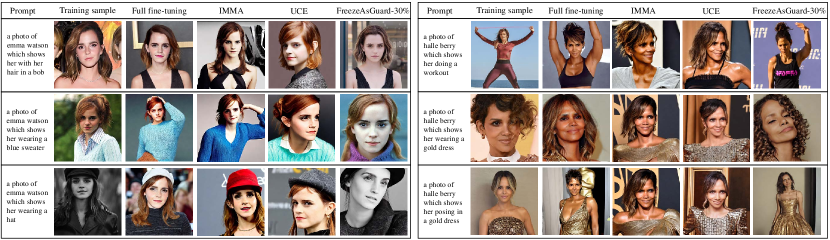
Figure 7: Qualitative examples of generated images in illegal domains of 10 subjects in FF25 dataset, after applying FreezeAsGuard-30% to fine-tuning SD v1.5. Each prompt adopts the same seed for generation. More image examples are in Appendix G.

4.2 Qualitative Examples of Generated Images

Most existing metrics cannot precisely reflect the image quality perceived by humans [31; 17]. Instead, being similar to those shown in Figure 2, we show more qualitative image examples in Figure 7, which show that FreezeAsGuard effectively prevents the generated images from being recognized as the target subjects by human perception. Meanwhile, the fine-tuned model can still generate detailed background content and subjects’ postures aligned with the prompt, indicating that the mitigation power is highly selective and focuses only on subjects’ faces. In contrast, although UCE [25] and IMMA [59] can unlearn the knowledge of illegal domains by modifying the model weights, the illegal user can still relearn such knowledge via fine-tuning and the fine-tuned model can still generate images with decent quality. The key reason is that these unlearning methods do not have any restriction on the fine-tuning process, which instead, can be effectively regulated by FreezeAsGuard via tensor freezing.

Besides, freezing more model tensors could reduce overfitting in illegal domains and possibly improve the quality of fine-tuning. As shown in Figure 8, we pick some examples that can be easily mitigated by FreezeAsGuard with a very low $\rho$ (e.g., 1%). Then, when $\rho$ increases from 1% to 80%, FreezeAsGuard exhibits constant mitigation power despite the potentially less model overfitting. This is because the overfitting reduction is implicitly incorporated into mask learning by simulating different selections of tensor freezing, and the mitigation power hence overweighs the overfitting reduction.

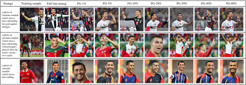
Figure 8: Qualitative image examples after applying FreezeAsGuard to fine-tuning SD v1.5, with different freezing ratios in illegal domains. Each row adopts the same seed for generation.

4.3 Mitigation Power with Different Illegal Domain Scales

We randomly pick images from 2, 5, and 10 subjects in FF25 dataset, as the illegal domain. As shown in Table 4, FreezeAsGuard can reduce the FID of generated images by up to 14% compared to full FT. In comparison, UCE exhibits no mitigation power in some cases since fine-tuning can relearn the unlearned knowledge in illegal domains. IMMA aggressively modifies the weights and results in significant performance drops in innocent domains. With more subjects in illegal domain, the difference of mitigation between FreezeAsGuard and random freezing becomes smaller, because more subjects correspond to more adaptation-critical tensors, and random freezing is more likely to cover them.

4.4 Different Innocent Domains

It is possible that illegal domains and innocent domains share some critical parameters in common. However, as shown in Table 5, FreezeAsGuard maximally retains the adaptation performance in different innocent domains, with on-par or even better image quality compared to UCE and IMMA. In some cases, the CLIP scores of generated images are better than the training samples, possibly because the fine-tuned model finds a shortcut that deceives the pre-trained CLIP model. We are then motivated to check the qualitative results as shown in Figure 9. The generated images are either similar to training samples, or more colorful and contain more details. Besides, the generated images are not perfectly aligned with prompts, and we attribute these errors to the limitation of open-sourced SD models. These errors can be mitigated with other larger diffusion models, such as DALL-E 3 [10] and Imagen2 [12].

Method	2 subjects (seed 1)		2 subjects (seed 2)		5 subjects		10 subjects
	Illegal FID ($\downarrow$)	Innocent CLIP ($\uparrow$)	Illegal FID ($\downarrow$)	Innocent CLIP ($\uparrow$)	Illegal FID ($\downarrow$)	Innocent CLIP ($\uparrow$)	Illegal FID ($\downarrow$)	Innocent CLIP ($\uparrow$)
Full FT	139.20	32.83	135.61	32.83	127.38	32.83	143.58	32.83
UCE	138.39	30.74	147.35	30.27	131.27	30.27	151.53	30.25
IMMA	139.88	30.03	145.39	29.81	129.60	28.99	148.05	28.71
Random-20%	139.04	29.80	142.72	29.80	135.48	29.80	152.65	29.80
FreezeAsGuard-20%	151.30	30.31	153.90	30.10	135.85	31.12	156.09	30.26
Random-30%	138.16	28.92	142.64	28.92	136.65	28.92	152.21	28.92
FreezeAsGuard-30%	146.30	31.49	153.00	30.29	138.09	30.48	155.98	30.47

Table 4: Mitigation power in illegal domains with different scales (as numbers of subjects in FF25 dataset) and innocent domains (Logo dataset)

Method	Logo dataset		Clothes dataset
	CLIP ($\uparrow$)	TOPIQ ($\uparrow$)	CLIP ($\uparrow$)	TOPIQ ($\uparrow$)
GT	31.24	-	29.63	-
Full FT	32.83	0.097	32.84	0.059
UCE	30.27	0.088	32.47	0.070
IMMA	28.99	0.097	31.01	0.065
R-10%	30.28	0.091	32.33	0.055
FG-10%	31.41	0.100	31.98	0.065
R-20%	30.36	0.093	32.44	0.064
FG-20%	31.12	0.103	31.73	0.062

Table 5: Results on different innocent data domains with photos of 5 subjects as the illegal domain (GT: Ground Truth, FG: FreezeAsGuard)

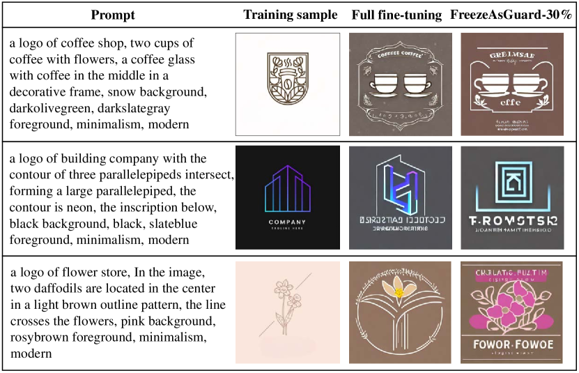
Figure 9: Generated image examples on the logo dataset as the innocent domain

4.5 Different Diffusion Models

We apply FreezeAsGuard to three different SD models. As shown in Table 6, FreezeAsGuard constantly outperforms baseline schemes on all diffusion models. According to the full fine-tuning performance, SD v1.4 and v1.5 are generally stronger than v2.1. Accordingly, FreezeAsGuard’s retaining power in the innocent domain is slightly better for v1.4 and v1.5 models. We hypothesize that better pre-trained models have more modularized knowledge distribution over model parameters, and hence allow FreezeAsGuard to freeze them without affecting innocent domains.

Method	Stable Diffusion v1.4		Stable Diffusion v1.5		Stable Diffusion v2.1
	Illegal FID ($\downarrow$)	Innocent CLIP ($\uparrow$)	Illegal FID ($\downarrow$)	Innocent CLIP ($\uparrow$)	Illegal FID ($\downarrow$)	Innocent CLIP ($\uparrow$)
Full FT	146.03	33.26	143.58	32.83	148.37	32.44
UCE	151.06	30.12	151.53	30.27	152.77	27.48
IMMA	150.49	29.07	148.05	28.71	149.49	26.89
Random-20%	151.42	30.00	152.65	29.80	152.52	28.43
FreezeAsGuard-20%	156.11	30.27	156.09	30.26	155.47	28.47

Table 6: Quantitative results on illegal (10 subjects in FF25 dataset) and innocent domains (Logo dataset) using different diffusion models

5 Conclusion & Broader Impact

In this paper, we present FreezeAsGuard, a new technique for mitigating illegal adaptation of diffusion models by freezing model tensors that are adaptation-critical only for illegal domains. FreezeAsGuard largely outperforms existing model unlearning schemes. Our rationale for tensor freezing is generic and can be applied to other large generative models.

Appendix A Vectorizing the Gradient Calculations in Bilevel Optimization

In practice, the solutions to bilevel optimization in Eq. (2) and Eq. (3) can usually be approximated through gradient-based optimizers. However, existing deep learning APIs (e.g., TensorFlow and PyTorch) maintain model tensors in either list or dictionary-like structures, and hence the gradient calculation for Eq. (4) cannot be automatically vectorized with the mask vector $\mathbf{m}$. To enhance the compute efficiency, we decompose the process of gradient calculation and assign the majority of compute workload to the highly optimized APIs.

Specifically, in mask learning in the upper-level loop specified in Eq. (5), $\mathcal{L}_{upper}$’s gradient w.r.t a model tensor’s $w_{i}$ can be decomposed via the chain rule as:

$$\frac{\partial{\mathcal{L}_{upper}}}{\partial{w_{i}}}=\left<\frac{\partial{\mathcal{L}_{upper}}}{\partial{\theta(m)_{i}}},\frac{\partial{\theta(m)_{i}}}{m_{i}}\right>\frac{\partial m_{i}}{\partial w_{i}}=\left<\frac{\partial{\mathcal{L}_{upper}}}{\partial{\theta(m)_{i}}},\theta_{pre}^{(i)}-\theta_{ft}^{(i)}\right>\frac{1}{T}\sigma\left(\frac{w_{i}}{T}\right)\sigma\left(1-\frac{w_{i}}{T}\right),$$ (11)

where $<\cdot,\cdot>$ denotes the inner product. The calculation of the gradient component, i.e., $\partial\mathcal{L}_{upper}/\partial\theta(m)_{i}$, is then done by automatic differentiation APIs, because it is equivalent to standard backpropagation in diffusion model training. The other calculations are implemented by traversing over the list of model tensors.

Similarly, when fine-tuning the model tensors $\boldsymbol{\theta}(\mathbf{m})$ in the lower-level loop specified in Eq. (7), we also decompose its gradient calculation process. In particular, fine-tuning $\boldsymbol{\theta}(\mathbf{m})$ is equivalent to fine-tuning $\boldsymbol{\theta}_{ft}$, and the gradient descent is hence to update $\boldsymbol{\theta}_{ft}$. More specifically, the gradient of a given tensor $i$ is:

$$\frac{\partial\mathcal{L}_{lower}}{\partial\theta_{ft}^{(i)}}=\frac{\partial\mathcal{L}_{lower}}{\partial\theta(m)_{i}}\frac{\partial\theta(m)_{i}}{\partial\theta_{ft}^{(i)}}=\frac{\partial\mathcal{L}_{lower}}{\partial\theta(m)_{i}}(1-m_{i}),$$ (12)

where we leave $\partial\mathcal{L}_{lower}/\partial\theta_{ft}^{(i)}$ to automatic differentiation APIs because it is equivalent to standard backpropagation in diffusion model training. Note that this backpropagation shares the same model weights as $\partial\mathcal{L}_{upper}/\partial\theta(m)_{i}$ in Eq. (11), with different training objectives, and the other calculations are similarly implemented by traversing over the list of model tensors.

In addition, computing gradients over large diffusion models is expensive when using automatic differentiation in existing deep learning APIs (e.g., PyTorch and TensorFlow). Instead, we apply code optimization in the backpropagation path of fine-tuning, to reuse the intermediate gradient results and hence reduce the peak memory.

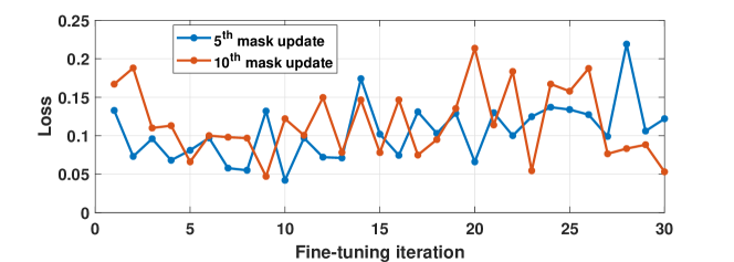
Figure 10: Fine-tuning loss after the 5th and 10th mask updates during bilevel optimization

Appendix B Deciding the Number of Fine-tuning Iterations in Bilevel Optimization

As shown in Figure 10, we observe that in the lower-level loop of model fine-tuning, the fine-tuning loss typically drops fast in the first 5-10 iterations, but then starts to violently fluctuate. Such quick drop of loss at the initial stage of fine-tuning is particularly common in fine-tuning large generative models, because the difference between the fine-tuned and pre-trained weights can be so small that only a few weight updates can get close [55]. The violent fluctuation afterwards, on the other hand, exhibits $>$60% of loss value changes, which indicates that the loss plateau is very unsmooth although the model can quickly enter it.

Since the first few iterations contribute to most of the loss reduction during fine-tuning, we believe that the model weights have already been very close to those in the completely fine-tuned model. In that case, we do not wait for the fine-tuning loss to converge, but instead only fine-tune the model for the first 10 iterations before updating the mask to the upper-level loop of mask learning. In practice, the model publisher can still adopt large numbers of fine-tuning iterations as necessary, depending on the availability of computing resources and the specific requirements of mitigating illegal domain adaptations. Similar approximation schemes are also adopted in existing work [46, 59] to solve bilevel optimization problems, but most of them aggressively set the interval to be only one iteration, leading to arguably high approximation errors.

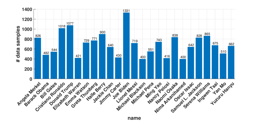
Figure 11: Statistics of the Famous-Figures-25 dataset

Appendix C Details of the Famous-Figures-25 (FF25) Dataset

Our FF25 dataset contains 8,703 portrait images of 25 public figures and the corresponding text descriptions. All the images were crawled from publicly available sources on the Web. These 25 subjects include politicians, movie stars, writers, athletes and businessmen, with diverse genders, races, and career domains. As shown in Figure 11, the dataset contains 400-1,300 images of each subject.

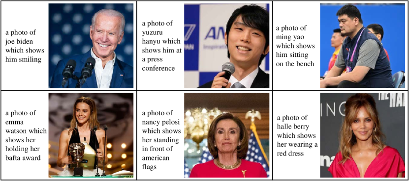
Figure 12: Examples of portrait images in the Famous-Figures-25 dataset

When crawling images on the web, we only consider images that 1) has a resolution higher than 512$\times$512 and 2) contains $>$3 faces detected by OpenCV face recognition API [13] as valid. Each raw image is then center-cropped to a resolution of 512$\times$512. For each image, we use a pre-trained BLIP2 image captioning model [38] to generate the corresponding text description, and prompt BLIP2 with the input of “a photo of <person_name> which shows” to avoid hallucination. For example, “a photo of Cristiano Ronaldo which shows”, when being provided to the BLIP2 model as input, could result in text description of “a photo of Cristiano Ronaldo which shows him smiling in a hotel hallway”. More sample images and their corresponding text descriptions are shown in Figure 12.

Appendix D Source Code Repository

We have packed all the source codes of FreezeAsGuard into the a .zip file and provided the file in the supplementary material. Please refer to the README.md file in the code repository for details about the source codes. In the README.md file, we also provided an anonymous link to our self-collected FF25 dataset.

Appendix E Sample Images of Datasets as Innocent Domains

The Logo dataset [4] contains minimalist designs of logo images with highly detailed text descriptions. As shown in Figure 14, the logos can correspond to different types of businesses, such as restaurants, coffee shops, and e-shops. The text description specifies the shape, color, and position of every object that should be included in the logo. Most images are near square and the logo is centered, and these images can hence be safely center-cropped to the standard resolution of 512$\times$512 for fine-tuning (being similar to those in the FF25 dataset).

Similarly, the Clothes dataset [3] contains images of fashion products with highly detailed text descriptions. As shown in Figure 14, the products include clothes (e.g., coats and T-shirts) and other wearings (e.g., scarves). The text description can specify not only direct visual information (e.g., color and shape) but also texture information (e.g., soft cotton and recycled wool). Despite having diverse resolutions, most products are centered on the images and can be first center-cropped and then rescaled to achieve 512$\times$512 for fine-tuning (being similar to those in the FF25 dataset).

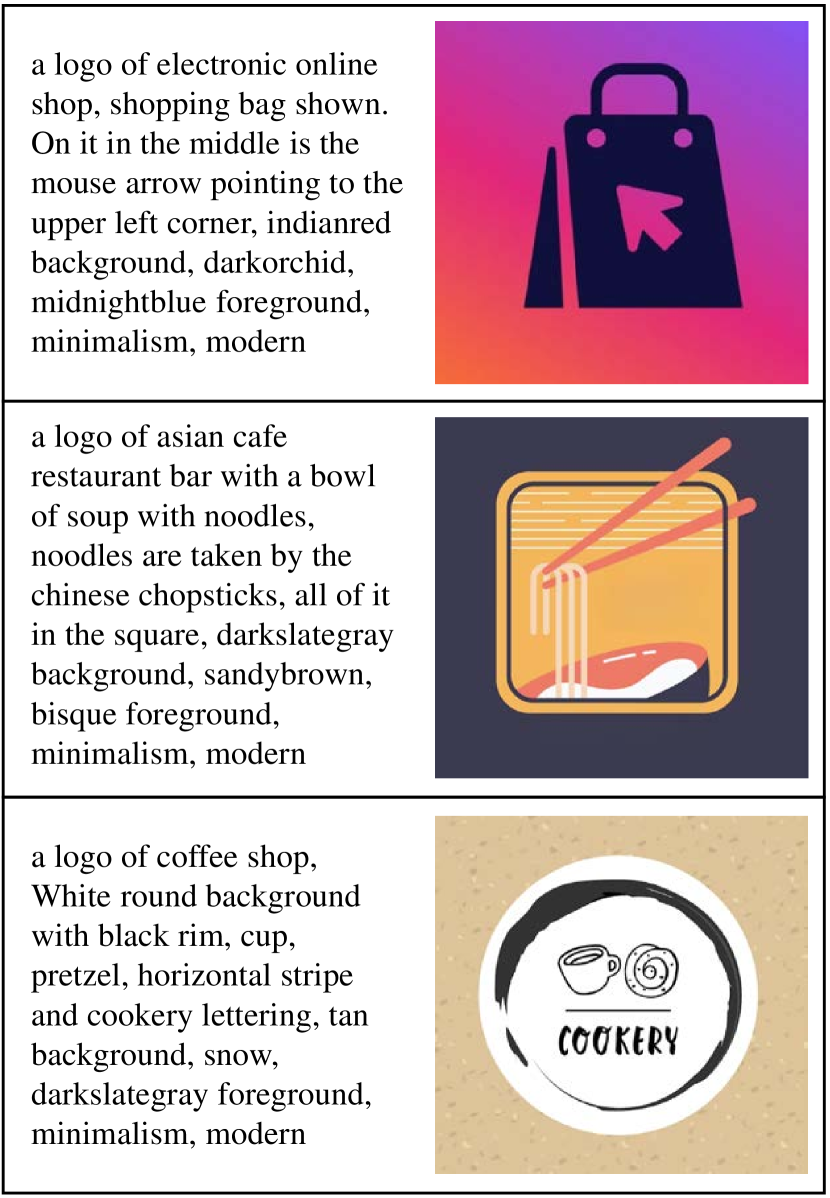
Figure 13: Examples in Logo dataset

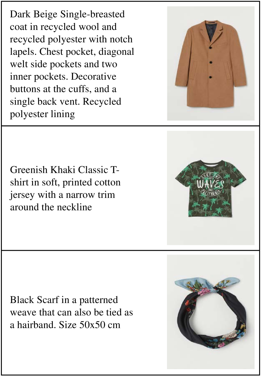
Figure 14: Examples in Clothes dataset

Appendix F Details of Evaluation Setup

For subjects in illegal domains (i.e., public figures in the FF25 dataset) and innocent domains (i.e., subjects in Logo and Clothes datasets), we use 100 images of each subject for mask learning. The remaining data samples in the FF25 dataset are used for illegal model fine-tuning. Note that, to mitigate model adaptation in a specific illegal domain (e.g., a specific public figure), we will need to use data samples in the same domain for mask learning. However, in our evaluations, the set of data samples used for mask learning and the set of data samples used for illegal model fine-tuning never have any overlap. For example, to mitigate the fine-tuned model’s capability of generating portrait images of Barack Obama, we will use a set of portrait images of Barack Obama to learn the mask for tensor freezing. Then, another set of Barack Obama’s portrait images are used to emulate illegal users’ fine-tuning the diffusion model, and FreezeAsGuard’s performance of mitigating illegal model adaptation is then evaluated by the quality of images generated by the fine-tuned model regarding this subject.

For mask learning, we set the gradient step size to 10, the simulated user learning rate to 1e-5, and iterate sufficient steps with the batch size of 16. The temperature for the mask’s continuous form is set to 0.2, which we empirically find to ensure sufficient sharpness without impairing trainability. When fine-tuning the diffusion model as an illegal user, we adopt a learning rate of 1e-5 and the batch size of 4 with Adam [35] optimizer, to fine-tune 2,000 iterations on subject’s data samples. Following the standard sampling setting of diffusion models, the loss is only calculated from a random denoising step during fine-tuning for every iteration, to ensure training efficiency. For image generation, we adopt the PNDMScheduler [34] and proceed with 50 denoising steps for sufficient image quality.

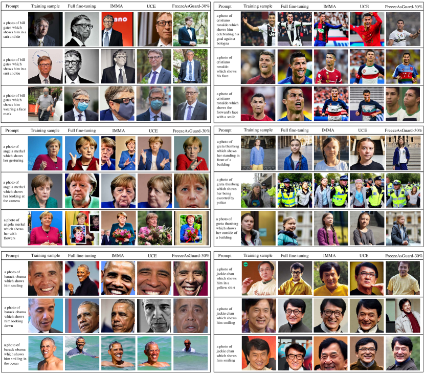
Figure 15: Qualitative image generation performance after applying FreezeAsGuard-30% to Stable Diffusion v1.5 on illegal domains, where each prompt adopts the same seed for generation

Appendix G More Qualitative Examples of Images Generated by the Fine-tuned Model

The image quality degradation introduced by FreezeAsGuard can be from different perspectives. As shown in Figure 15, in most cases, such as for Angela Merkel and Barack Obama, the distortion is exhibited as stretched faces or exaggerated emotions which make the subject unrecognizable. In some other cases, such as the third row of Cristiano Ronaldo’s photos, the generated image contains unrealistic duplication of subjects. Moreover, for the third row of Bill Gates’s photos, the subject in the generated image with FreezeAsGuard is not wearing a mask, which is not aligned with the prompt. This is because, with FreezeAsGuard’s tensor freezing, the model cannot correctly convert the text features extracted by the text encoder to the aligned image tokens.

Appendix H The Learned Selection of Frozen Tensors

In Figure 16, we present the learned masks with different freezing ratios on 10 subject’s portrait images as the illegal domain and the logo dataset as the innocent domain. The distribution of the frozen tensors is never uniform over all freezing ratios. We found that most of the selected tensors are the kernel tensors of conv_in layers in the UNet. As the freezing ratio increases, more bias tensors are selected to freeze.

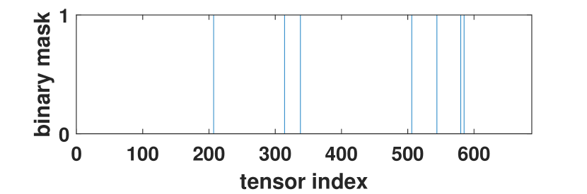
(a) freezing ratio = 1%

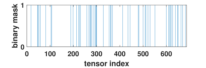
(b) freezing ratio = 5%

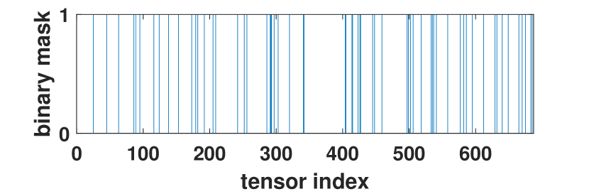
(c) freezing ratio = 10%

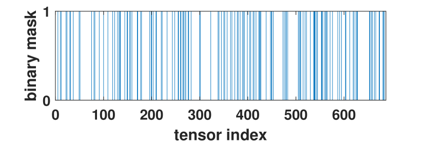
(d) freezing ratio = 20%

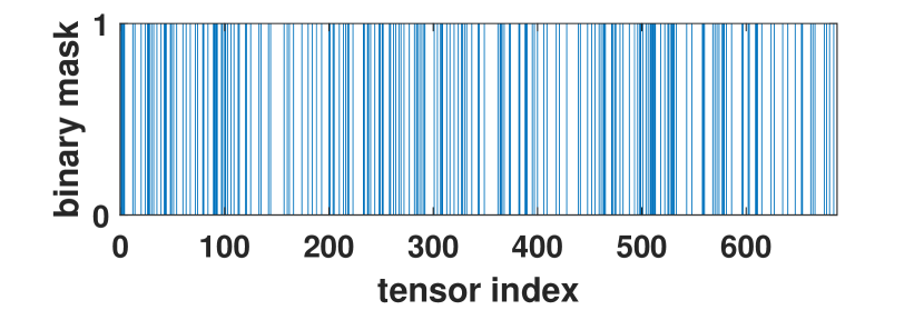
(e) freezing ratio = 30%

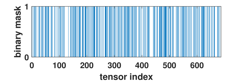
(f) freezing ratio = 40%

Figure 16: Learned binary masks with different freezing ratios (1 means to freeze)

References

- fal [2022] some-notes-on-the-stable-diffusion-safety-filter. https://vickiboykis.com/2022/11/18/some-notes-on-the-stable-diffusion-safety-filter/, 2022.
- aut [2023] Autocrawler. https://github.com/YoongiKim/AutoCrawler, 2023.
- clo [2023] H&m clothes dataset. https://huggingface.co/datasets/wbensvage/clothes_desc, 2023.
- log [2023] modern-logo-v4 dataset. https://huggingface.co/datasets/logo-wizard/modern-logo-dataset, 2023.
- pok [2023] pokemon dataset. https://huggingface.co/datasets/lambdalabs/pokemon-blip-captions, 2023.
- saf [2023] stable-diffusion-safety-checker. https://huggingface.co/CompVis/stable-diffusion-safety-checker, 2023.
- sd1 [2023a] stable diffusion v1.4. https://huggingface.co/CompVis/stable-diffusion-v1-4, 2023a.
- sd1 [2023b] stable diffusion v1.5. https://huggingface.co/runwayml/stable-diffusion-v1-5, 2023b.
- sd2 [2023] stable diffusion v2.1. https://huggingface.co/runwayml/stable-diffusion-v1-5, 2023.
- dal [2024] Dall-e 3. https://openai.com/dall-e-3, 2024.
- dif [2024] Diffusion wallpaper. https://serp.ai/tools/diffusion-wallpaper/, 2024.
- ima [2024] Imagen 2. https://deepmind.google/technologies/imagen-2/, 2024.
- ope [2024] Opencv face recognition. https://opencv.org/opencv-face-recognition/, 2024.
- Chefer et al. [2023] H. Chefer, O. Lang, M. Geva, V. Polosukhin, A. Shocher, M. Irani, I. Mosseri, and L. Wolf. The hidden language of diffusion models. arXiv preprint arXiv:2306.00966, 2023.
- Chen et al. [2024] C. Chen, J. Mo, J. Hou, H. Wu, L. Liao, W. Sun, Q. Yan, and W. Lin. Topiq: A top-down approach from semantics to distortions for image quality assessment. IEEE Transactions on Image Processing, 2024.
- Chen et al. [2019] Y. Chen, B. Chen, X. He, C. Gao, Y. Li, J.-G. Lou, and Y. Wang. opt: Learn to regularize recommender models in finer levels. In Proceedings of the 25th ACM SIGKDD International Conference on Knowledge Discovery & Data Mining, pages 978–986, 2019.
- Cheon et al. [2021] M. Cheon, T. Vigier, L. Krasula, J. Lee, P. Le Callet, and J.-S. Lee. Ambiguity of objective image quality metrics: A new methodology for performance evaluation. Signal Processing: Image Communication, 93:116150, 2021.
- Cui et al. [2023a] Y. Cui, J. Ren, Y. Lin, H. Xu, P. He, Y. Xing, W. Fan, H. Liu, and J. Tang. Ft-shield: A watermark against unauthorized fine-tuning in text-to-image diffusion models. arXiv preprint arXiv:2310.02401, 2023a.
- Cui et al. [2023b] Y. Cui, J. Ren, H. Xu, P. He, H. Liu, L. Sun, and J. Tang. Diffusionshield: A watermark for copyright protection against generative diffusion models. arXiv preprint arXiv:2306.04642, 2023b.
- Derner and Batistič [2023] E. Derner and K. Batistič. Beyond the safeguards: Exploring the security risks of chatgpt. arXiv preprint arXiv:2305.08005, 2023.
- Fan et al. [2023] C. Fan, J. Liu, Y. Zhang, D. Wei, E. Wong, and S. Liu. Salun: Empowering machine unlearning via gradient-based weight saliency in both image classification and generation. arXiv preprint arXiv:2310.12508, 2023.
- Finn et al. [2017] C. Finn, P. Abbeel, and S. Levine. Model-agnostic meta-learning for fast adaptation of deep networks. In International conference on machine learning, pages 1126–1135. PMLR, 2017.
- Gal et al. [2022] R. Gal, Y. Alaluf, Y. Atzmon, O. Patashnik, A. H. Bermano, G. Chechik, and D. Cohen-Or. An image is worth one word: Personalizing text-to-image generation using textual inversion. arXiv preprint arXiv:2208.01618, 2022.
- Gamage et al. [2022] D. Gamage, P. Ghasiya, V. Bonagiri, M. E. Whiting, and K. Sasahara. Are deepfakes concerning? analyzing conversations of deepfakes on reddit and exploring societal implications. In Proceedings of the 2022 CHI Conference on Human Factors in Computing Systems, pages 1–19, 2022.
- Gandikota et al. [2024] R. Gandikota, H. Orgad, Y. Belinkov, J. Materzyńska, and D. Bau. Unified concept editing in diffusion models. In Proceedings of the IEEE/CVF Winter Conference on Applications of Computer Vision, pages 5111–5120, 2024.
- Gosse and Burkell [2020] C. Gosse and J. Burkell. Politics and porn: how news media characterizes problems presented by deepfakes. Critical Studies in Media Communication, 37(5):497–511, 2020.
- Harwell [2017] D. Harwell. Ai-generated child sex images spawn new nightmare for the web. The Wall Street Journal, 2017.
- Heikkilä [2022] M. Heikkilä. This artist is dominating ai-generated art. and he’s not happy about it. MIT Technology Review, 125(6):9–10, 2022.
- Hessel et al. [2021] J. Hessel, A. Holtzman, M. Forbes, R. L. Bras, and Y. Choi. Clipscore: A reference-free evaluation metric for image captioning. arXiv preprint arXiv:2104.08718, 2021.
- Heusel et al. [2017] M. Heusel, H. Ramsauer, T. Unterthiner, B. Nessler, and S. Hochreiter. Gans trained by a two time-scale update rule converge to a local nash equilibrium. Advances in neural information processing systems, 30, 2017.
- Hu et al. [2020] B. Hu, L. Li, J. Wu, and J. Qian. Subjective and objective quality assessment for image restoration: A critical survey. Signal Processing: Image Communication, 85:115839, 2020.
- Hu et al. [2021] E. J. Hu, Y. Shen, P. Wallis, Z. Allen-Zhu, Y. Li, S. Wang, L. Wang, and W. Chen. Lora: Low-rank adaptation of large language models. arXiv preprint arXiv:2106.09685, 2021.
- Hwang and Masud [2012] C.-L. Hwang and A. S. M. Masud. Multiple objective decision making—methods and applications: a state-of-the-art survey, volume 164. Springer Science & Business Media, 2012.
- Karras et al. [2022] T. Karras, M. Aittala, T. Aila, and S. Laine. Elucidating the design space of diffusion-based generative models. Advances in Neural Information Processing Systems, 35:26565–26577, 2022.
- Kingma and Ba [2014] D. P. Kingma and J. Ba. Adam: A method for stochastic optimization. arXiv preprint arXiv:1412.6980, 2014.
- Krizhevsky et al. [2009] A. Krizhevsky, G. Hinton, et al. Learning multiple layers of features from tiny images. 2009.
- Lee et al. [2018] N. Lee, T. Ajanthan, and P. H. Torr. Snip: Single-shot network pruning based on connection sensitivity. arXiv preprint arXiv:1810.02340, 2018.
- Li et al. [2023] J. Li, D. Li, S. Savarese, and S. Hoi. Blip-2: Bootstrapping language-image pre-training with frozen image encoders and large language models. In International conference on machine learning, pages 19730–19742. PMLR, 2023.
- Liu et al. [2018a] H. Liu, K. Simonyan, and Y. Yang. Darts: Differentiable architecture search. arXiv preprint arXiv:1806.09055, 2018a.
- Liu et al. [2021] L. Liu, S. Zhang, Z. Kuang, A. Zhou, J.-H. Xue, X. Wang, Y. Chen, W. Yang, Q. Liao, and W. Zhang. Group fisher pruning for practical network compression. In International Conference on Machine Learning, pages 7021–7032. PMLR, 2021.
- Liu et al. [2018b] Z. Liu, P. Luo, X. Wang, and X. Tang. Large-scale celebfaces attributes (celeba) dataset. Retrieved August, 15(2018):11, 2018b.
- Podell et al. [2023] D. Podell, Z. English, K. Lacey, A. Blattmann, T. Dockhorn, J. Müller, J. Penna, and R. Rombach. Sdxl: Improving latent diffusion models for high-resolution image synthesis. arXiv preprint arXiv:2307.01952, 2023.
- Rombach et al. [2022] R. Rombach, A. Blattmann, D. Lorenz, P. Esser, and B. Ommer. High-resolution image synthesis with latent diffusion models. In Proceedings of the IEEE/CVF conference on computer vision and pattern recognition, pages 10684–10695, 2022.
- Ronneberger et al. [2015] O. Ronneberger, P. Fischer, and T. Brox. U-net: Convolutional networks for biomedical image segmentation. In Medical image computing and computer-assisted intervention–MICCAI 2015: 18th international conference, Munich, Germany, October 5-9, 2015, proceedings, part III 18, pages 234–241. Springer, 2015.
- Royer et al. [2020] A. Royer, K. Bousmalis, S. Gouws, F. Bertsch, I. Mosseri, F. Cole, and K. Murphy. Xgan: Unsupervised image-to-image translation for many-to-many mappings. Domain Adaptation for Visual Understanding, pages 33–49, 2020.
- Ruiz et al. [2023] N. Ruiz, Y. Li, V. Jampani, Y. Pritch, M. Rubinstein, and K. Aberman. Dreambooth: Fine tuning text-to-image diffusion models for subject-driven generation. In Proceedings of the IEEE/CVF Conference on Computer Vision and Pattern Recognition, pages 22500–22510, 2023.
- Russakovsky et al. [2015] O. Russakovsky, J. Deng, H. Su, J. Krause, S. Satheesh, S. Ma, Z. Huang, A. Karpathy, A. Khosla, M. Bernstein, et al. Imagenet large scale visual recognition challenge. International journal of computer vision, 115:211–252, 2015.
- Schuhmann et al. [2022] C. Schuhmann, R. Beaumont, R. Vencu, C. Gordon, R. Wightman, M. Cherti, T. Coombes, A. Katta, C. Mullis, M. Wortsman, et al. Laion-5b: An open large-scale dataset for training next generation image-text models. Advances in Neural Information Processing Systems, 35:25278–25294, 2022.
- Shan et al. [2023] S. Shan, J. Cryan, E. Wenger, H. Zheng, R. Hanocka, and B. Y. Zhao. Glaze: Protecting artists from style mimicry by Text-to-Image models. In 32nd USENIX Security Symposium (USENIX Security 23), pages 2187–2204, 2023.
- Wang et al. [2003] Z. Wang, E. P. Simoncelli, and A. C. Bovik. Multiscale structural similarity for image quality assessment. In The Thrity-Seventh Asilomar Conference on Signals, Systems & Computers, 2003, volume 2, pages 1398–1402. Ieee, 2003.
- Webson and Pavlick [2021] A. Webson and E. Pavlick. Do prompt-based models really understand the meaning of their prompts? arXiv preprint arXiv:2109.01247, 2021.
- Wolf et al. [2019] T. Wolf, L. Debut, V. Sanh, J. Chaumond, C. Delangue, A. Moi, P. Cistac, T. Rault, R. Louf, M. Funtowicz, et al. Huggingface’s transformers: State-of-the-art natural language processing. arXiv preprint arXiv:1910.03771, 2019.
- Wu et al. [2024] J. Wu, T. Le, M. Hayat, and M. Harandi. Erasediff: Erasing data influence in diffusion models. arXiv preprint arXiv:2401.05779, 2024.
- Ye et al. [2023] X. Ye, H. Huang, J. An, and Y. Wang. Duaw: Data-free universal adversarial watermark against stable diffusion customization. arXiv preprint arXiv:2308.09889, 2023.
- Yu et al. [2023] L. Yu, B. Yu, H. Yu, F. Huang, and Y. Li. Language models are super mario: Absorbing abilities from homologous models as a free lunch. arXiv preprint arXiv:2311.03099, 2023.
- Zeiler and Fergus [2014] M. D. Zeiler and R. Fergus. Visualizing and understanding convolutional networks. In Computer Vision–ECCV 2014: 13th European Conference, Zurich, Switzerland, September 6-12, 2014, Proceedings, Part I 13, pages 818–833. Springer, 2014.
- Zhang et al. [2023] X. Zhang, R. Li, J. Yu, Y. Xu, W. Li, and J. Zhang. Editguard: Versatile image watermarking for tamper localization and copyright protection. arXiv preprint arXiv:2312.08883, 2023.
- Zhao et al. [2023] Y. Zhao, T. Pang, C. Du, X. Yang, N.-M. Cheung, and M. Lin. A recipe for watermarking diffusion models. arXiv preprint arXiv:2303.10137, 2023.
- Zheng and Yeh [2023] Y. Zheng and R. A. Yeh. Imma: Immunizing text-to-image models against malicious adaptation. arXiv preprint arXiv:2311.18815, 2023.