Distributed Continual Learning

Abstract

This work studies the intersection of continual and federated learning, in which independent agents face unique tasks in their environments and incrementally develop and share knowledge. We introduce a mathematical framework capturing the essential aspects of distributed continual learning, including agent model and statistical heterogeneity, continual distribution shift, network topology, and communication constraints. Operating on the thesis that distributed continual learning enhances individual agent performance over single-agent learning, we identify three modes of information exchange: data instances, full model parameters, and modular (partial) model parameters. We develop algorithms for each sharing mode and conduct extensive empirical investigations across various datasets, topology structures, and communication limits. Our findings reveal three key insights: sharing parameters is more efficient than sharing data as tasks become more complex; modular parameter sharing yields the best performance while minimizing communication costs; and combining sharing modes can cumulatively improve performance.

1 Introduction

Throughout human history, collective intelligence has driven significant scientific and technological advancements [6, 12]. The pooling and exchange of knowledge among individuals have often led to outcomes that far exceed the capabilities of isolated efforts. This collective principle is now reflected in contemporary machine learning research, where combining data [24, 5] and computational resources [4, 13] can produce significantly more capable models. However, training such large-scale foundation models typically requires a high degrees of coordination among agents (e.g., through a central server), and is only done once due to costs.

In contrast, we envision a future of ubiquitous embodied agents in the wild, such as vehicles in different cities or service robots in various homes. While foundation models provide a strong starting point, these robots need to continually learn new skills for their specific contexts. We posit that the selective sharing of knowledge among these agents through a communication network can substantially complement and enhance individual learning [56]. For example, consider a fleet of household robots deployed in homes across the nation. Commonalities across house layout, possessions, user preferences, etc. would enable one robot to benefit from the experience of others, improving collective performance and accelerating learning, yet individual aspects of each home and owner still require personalization of each robot. Despite its potential, this domain presents several key challenges inherited from related fields, including:

• Agent Heterogeneity: The diversity in agent functional forms, such as varying neural network architectures and learning algorithms, as well as differing local data and tasks, necessitate consideration of what form of knowledge to share and under what assumptions about agent commonality.

• Continual Adaptation: Algorithms for learning and sharing must facilitate ongoing skill acquisition and adaptation while retaining previously learned knowledge.

• Selective Transfer: Constraints on communication budgets and frequency necessitate efficient and selective knowledge transfer.

• Arbitrary Topologies: Sharing algorithms must be distributed and able to operate effectively in arbitrary communication topologies.

To address these challenges, we first formalize a mathematical framework for this problem of distributed continual learning (DCL), which encapsulates the essential aspects of this emerging field [56]. Within this framework, we identify three fundamental modes of knowledge exchange: data instances, full model parameters, and partial (modular) parameter sharing, each with its own trade-offs and benefits. We then develop selective methods tailored to each mode and conduct extensive experiments to highlight their strengths across datasets, communications topologies, and constraints.

Our contributions are as follows:

• Comprehensive Framework: We present a mathematical framework for distributed continual learning (DCL) that integrates features from several related fields.

• Selective Algorithms: We develop and analyze algorithms for three distinct modes of sharing: data instances, full model parameters, and partial (modular) parameter sharing.

• Empirical Insights: Our extensive empirical studies reveal that (1) parameter sharing is more efficient as tasks become more complex, (2) modular parameter sharing provides the best performance with minimal communication, and (3) combining sharing modes inherits the benefits of each mode.

• Baselines and Evaluation Protocols: We provide competitive sharing baselines and emphasize the importance of a robust evaluation protocol for future research in DCL, taking into account the hidden cost of communication and realistic considerations, such as agent model heterogeneity.

2 Related Work

The problem of distributed continual learning is related to several other topics, overviewed below:

Federated learning

Traditional federated learning [35, 26] focuses on training one global model using i.i.d data distributed across edge devices. More recent methods address challenges associated with non-i.i.d data among clients [27, 30, 28, 63, 32, 57], continual learning [64, 54], and decentralized architectures [59, 62]. These works typically compare themselves against other federated methods. Our work extends these concepts by incorporating both continual and distributed learning within a federated framework and comparing federated learning against other modes of sharing.

Continual Learning

Continual learning (CL) [50, 3, 44] aims to develop models capable of learning new tasks without forgetting the knowledge of past tasks. To combat catastrophic forgetting [34], methods have used regularization to limit drastic changes to network parameters during successive learning [20, 67, 29], rehearsal strategies that maintain a small subset of past data for periodic retraining [46, 17, 31], preservation of critical network nodes and pathways [18], and architectural modification strategies to add parameters and capacity for new tasks [51, 65, 49, 66]. Recent work has shown the benefits of using modular representations for architectural modification [40, 21, 37, 23, 38]. These methods decompose a neural network into independent and reusable knowledge components, for example, through neural block modules [40] or tensor factorization [23]. In a CL setting, modular representations allow for the selective reuse of prior knowledge and expansion as required [65, 36, 39, 37]. Modular learning is particularly relevant to this work as it provides a principled way to organize learned information into reusable components that can be shared between agents.

Multi-agent Systems

Research on distributed and multi-agent systems [9, 58, 25] spans several decades, focusing on applications in planning [8, 10], control [45, 2, 22, 14], and game theory [52]. Unlike our work, these systems often aim to solve a single shared task or manage agent behavior [58]. Nonetheless, considerations in multi-agent systems including network topology, communication constrain, and coordination requirements help to inform our formalism.

Distributed Continual Learning

Relatively few works have explored continual learning in distributed or multi-agent settings. An early work in distributed continual learning by Rostami et al. [47] tackles the problem using shallow factorized models, framing it as distributed dictionary optimization which requires that neighboring agents have similar knowledge bases. Subsequent work [41] extends this approach by allowing each agent to maintain some local expertise in addition to globally shared knowledge. However, this type of sharing is not selective as it fails to consider the transferability of knowledge between agents, and more importantly, it is restricted to simple parametric models (e.g., logistic regression) and thus not suitable for modern neural networks. More recent approaches allow task-specific transfer of knowledge via modulating masks [42] or lightweight heads [15]. However, these methods require all agents to share the same network backbone. Our modular sharing, on the other hand, affords the flexibility of model heterogeneity between agents. Furthermore, these works typically compare themselves against single-agent baselines instead of other sharing modes, and completely ignore the hidden cost of communication and other practical considerations including model heterogeneity. Our work aims to provide more competitive baselines, and more rigorous evaluation for future DCL research.

3 Distributed Continual Learning Framework

We now formalize the idea of distributed continual learning (DCL), with an emphasis on practical considerations such as supporting heterogeneous agents and communication constraints. Related works on DCL, described above, have explored variations of the problem; here we specify a framework that integrates and formalizes ideas from these works to unify them. Our framework consists of a directed graph $\mathcal{G}=\{A,E\}$ of $|A|$ nodes (agents) and $|E|$ edges that represent communication connections between agents. The collective of agents $A$ face a set of tasks $\mathcal{T}$, where each task $\mathcal{T}^{(t)}$ is a supervised learning problem with data $X^{(t)}\subseteq\mathcal{X}^{(t)}$ and labels $Y^{(t)}\subseteq\mathcal{Y}^{(t)}$ drawn from some data distribution for that task $\{\mathcal{X}^{(t)},\mathcal{Y}^{(t)}\}\sim\mathcal{T}^{(t)}$. Each agent $\mathrm{a}_{i}$ has a local view over this task space and faces a subset $\mathcal{T}_{i}\subseteq\mathcal{T}$ of these tasks. For example, robots in home versus commercial kitchens would share some tasks, but other tasks differ between the settings. Note that $\{\mathcal{T}_{i}\}_{i=1}^{|A|}$ covers $\mathcal{T}$.

Rather than learning all tasks en masse, each agent faces the tasks $\mathcal{T}_{i}$ in series: $\mathcal{T}_{i}^{(1)},\mathcal{T}_{i}^{(2)},\ldots,\mathcal{T}^{(t)}_{i},\ldots$, over its lifetime. Agent $\mathrm{a}_{i}$ learning task $\mathcal{T}^{(t)}_{i}$ corresponds to estimating parameters $\theta_{i}^{(t)}$ for a model $f_{\theta_{i}}^{(t)}:\mathcal{X}^{(t)}\mapsto\mathcal{Y}^{(t)}$ by solving a risk minimization problem with loss $\mathcal{L}_{i}^{(t)}\big{(}f^{(t)}_{\theta_{i}}(X^{(t)}),Y^{(t)}\big{)}$. Once task $\mathcal{T}^{(t)}\in\mathcal{T}_{i}$ is seen by the collective, agent $\mathrm{a}_{i}$ may be evaluated on it at any time, and so agents must retain knowledge of previous tasks. For two agents $\mathrm{a}_{i}$ and $\mathrm{a}_{j}$, note that their respective task sets $\mathcal{T}_{i}$ and $\mathcal{T}_{j}$ are not necessarily disjoint, and so may or may not overlap and share identical or related tasks. The task similarity $S(\mathcal{T}_{i},\mathcal{T}_{j})$ can be characterized using any measures of statistical difference between distributions, e.g., KL divergence [7].

The goal is for the agent collective to learn models for all tasks; since tasks may overlap or be related between agents, there is incentive for them to maximize performance by transferring knowledge from their previous tasks and across agents. Through the network $\mathcal{G}$, agent $\mathrm{a_{i}}$ can find other agents such as $\mathrm{a_{j}}$ who share similar tasks, allowing them to learn from each other. Each edge $e_{ij}$ represents a communication connection between agents $\mathrm{a}_{i}$ and $\mathrm{a}_{j}$, and, for realism, has a set budget $\mathtt{b}_{ij}$ of the maximum number of tokens allowed per communication and a permitted communication frequency $\mathtt{f}_{ij}$. The overall objective of the multi-agent collective can therefore be given by the cumulative expected loss of all agents over their task distributions, given the knowledge they are able to share:

$$\begin{split}\min_{\Theta_{1},\ldots\Theta_{|\!A\!|}}\sum_{\mathcal{T}^{(t)}\in\mathcal{T}}\sum_{\mathrm{a}_{i}\in A}\mathbb{E}_{(X^{(t)},Y^{(t)})\sim\mathcal{T}^{(t)}}\ \Pr(\mathcal{T}^{(t)}\!\mid\mathcal{T}_{i})\cdot\mathcal{L}_{i}^{(t)}\!\left(f^{(t)}_{\theta_{i}}(X^{(t)}),Y^{(t)}\mid\mathcal{K}_{i}\right)\\ \mbox{s.t. }\mathcal{K}_{i}=\textstyle{\bigcup_{j=1}^{|A|}K_{j,i}}\mbox{ and }\mathrm{size}(K_{j,i})\leq\mathrm{b}_{ji}\cdot\mathrm{f}_{ji}\cdot C\ \ \forall\{j|1\leq j\leq|A|,j\neq i\}\enspace,\end{split}$$ (1)

where $\Theta_{i}$ is all learned parameters for agent $\mathrm{a}_{i}$, $\mathcal{K}_{i}$ represents the set of knowledge $\mathrm{a}_{i}$ accumulated from other agents, $K_{j,i}$ is the knowledge sent from $\mathrm{a}_{j}$ to $\mathrm{a}_{i}$ (with $K_{i,i}=\emptyset$), and $C$ is a global clock counter for all communications that starts at 0 and increments each time agents receive a task.

Consequently, because the amount of transfer between agents is constrained by the communication bandwidth and frequency in Equation 1, the agents necessarily must be efficient in transferring knowledge to maximize collective performance. Since tasks are experienced sequentially by the agents, the ability to optimize this objective improves over time, as $C$ increases. Note also that this objective includes zero-shot performance on tasks that are unseen by an agent, but those unseen tasks may or may not be encountered by other agents in the collective.

This framework features several key characteristics that make this a challenging and realistic problem:

• Model heterogeneity: Agents might be functionally different (e.g., neural network architectures, learning methods, etc.) Compatibility is assumed only through the information $K_{ij}$ transferred.

• Task and data heterogeneity: Agents observe task distributions $\mathcal{T}_{i}$ and data that are local.

• Continual learning: Agents must solve new tasks over time, necessitating the adaptation of the $\Theta_{i}$’s. Agents may be evaluated on any task at any time, necessitating retention. The framework could support task- or class-incremental learning [61], depending on how the tasks $\mathcal{T}$ are formulated.

• Collaborative transfer: Collaboration provides a mechanism for agents to share information to improve collective performance, and could be either sender- or receiver-initiated.

• Communication constraints: The framework enforces realistic constraints on communication bandwidth $\mathtt{b}$ and frequency $\mathtt{f}$, which may differ by application. For example, embedded devices may send frequent but small updates (high $\mathtt{f}$, low $\mathtt{b}$), while satellites may limit both due to power.

• Arbitrary topology: Unlike the centralized server-client model of traditional federated learning, our framework supports agents connected in an arbitrary graph, potentially based on geolocation.

This framework unifies a variety of existing works on related problems, which can be specified as various assumptions on optimizing Eq. 1. For example, single-agent continual learning optimizes the $\mathcal{L}_{i}^{(t)}$’s independently under the assumption that $\mathcal{K}_{i}=\emptyset$. Rostami et al. [47] and Mohammadi and Kolouri [41] explore a variant assuming a factorized model for $K$ and unlimited communication. Ge et al. [15] assume a static shared backbone among all agents and share task-specific heads, biases, and task clusters as $K$, again under unlimited communication.

4 Modes of Knowledge Sharing

Prior works in continual [50, 3, 44] and distributed learning [47, 41, 42, 15] have explored some aspects of how to optimize Eq. 1 but largely ignored the form and constraint on $\mathcal{K}_{i}$. To bridge this gap, we focus on this fundamental challenge within Eq. 1 that has been under-investigated: what information should agents share in order to maximize collective performance? The communication constraints and heterogeneity among agents and tasks creates obstacles for addressing this challenge, including limiting the forms (modes) of information that can be conveyed. We study this problem by considering sharing of information at three different levels: instance-based, full-model, and partial-model. We first describe these modes, and then propose solutions to DCL with each.

Instance-based sharing of data (i.e., training examples) is the most generic mode, since it is model-agnostic and only requires agents to be compatible in their input data formats. The downside is that each data instance contains very limited information. So, this mode has low communication efficiency in general, although it may be efficient when only a few specific examples need to be shared.

Full-model sharing of full model parameters provides an efficient mechanism to share complete information among agents. Compression schemes could make transmission even more efficient, but the information content of the exchange would remain approximately the same. However, it also imparts strong assumptions that the agents’ models are directly compatible and that their task distributions are likely similar at any given time. This is most similar to federated methods that attempt to learn a unified model for all tasks in a distributed fashion.

Partial-model sharing of reusable model components represents a compromise between low-level data sharing and full model sharing. It relaxes assumptions on the agents’ model compatibility, requiring that they only be capable of utilizing the components within their model architecture, with that architecture and learning methods able to differ among agents. It also reduces the assumptions about common task distributions, allowing for selective sharing based on the similarity of the current task to some tasks in the past encountered by the collective. Although different forms of partial-model transfer are available that have been used for CL, e.g., factorized representations [47, 41], we impose an additional requirement—that the module be self-contained, so that they can be transferred independently. In contrast, factorized representations often have interdependencies (e.g., among model basis vectors), complicating the ability to share just one factor between agents. For this reason, we focus on transfer of self-contained modules, and in particular, modules that are compositional [36] in nature, thereby avoiding side effects from different combinations of modules.

4.1 Data Sharing

To determine what data to share in DCL, we explore a receiver-initiated approach, similar to active learning [53], where the receiving agent identifies gaps in its knowledge base and puts out requests for appropriate data from neighboring agents. Previous work has also explored sender-initiated models, such as training a sharing model that predicts the utility of an agent’s data to other agents based on estimated novelty [16]. Such sender-initiated methods assume the usefulness of data to other agents, rather than letting demand drive sharing, and hinge on frequent communication to train the sharing model. Conversely, other agents may have broader information on the data than an individual agent, and so sender-initiated models may fill gaps of which receiver agents were unaware.

In our receiver-initiated data sharing, $\mathtt{Recv}$, when agent $\mathrm{a}_{i}$ is learning task $\mathcal{T}^{(t)}$, it identifies $q$ difficult instances and requests more data that is similar. To identify the $\mathtt{q}$ hardest instances, we compute the cross entropy loss on the validation set $\mathcal{V}_{i}^{(1:t)}$ of all tasks encountered so far: $\mathcal{Q}_{i}^{(t)}=\operatorname*{arg\,max}_{I\subseteq\mathcal{V}_{i}^{(1:t)}}\sum_{(x,y)\in I}\mathcal{L}_{CE}(f_{\theta_{i}}(x),y)\mbox{ s.t. }|I|=\mathtt{q}$. Agent $\mathrm{a}_{i}$ then queries its neighbors $\mathcal{N}_{i}$ to return the $\mathtt{k}$ nearest instances to each query in $\mathcal{Q}_{i}^{(t)}$, based on a distance measure $d(\cdot)$. For $d(\cdot)$, we use the cosine distance of the latent representation from the penultimate layer of the neural network model $\phi_{\theta_{i}}(x)$. The result $\mathcal{R}_{j}^{(t)}(x)$ to a query $x$ computed by a sender $\mathrm{a}_{j}$ is the $k$ nearest instances in the sender database $\mathcal{\tilde{D}}_{j}^{(1:t)}$: $\mathcal{R}_{j}^{(t)}(x)=\operatorname*{arg\,min}_{R\subseteq\mathcal{\tilde{D}}_{j}^{(1:t)}}\sum_{(x^{\prime},y^{\prime})\in R}d(\phi_{\theta_{j}}(x),\phi_{\theta_{j}}(x^{\prime}))\mbox{ s.t. }|R|=\mathtt{k}$, where database $\mathcal{\tilde{D}}_{j}^{(1:t)}$ represents a select subset of $\mathrm{a}_{j}$’s training data from known tasks, such as stored in a replay buffer to avoid catastrophic forgetting [17]. The values of $\mathtt{q}$ and $\mathtt{k}$ are determined by the communication limit $\mathtt{b}$ of the network such that $\mathtt{b}=\mathtt{q}\mathtt{k}.$

We also implement a simpler sharing mechanism, $\mathtt{Simp}$, where the receiver requests data from certain classes, and the sender samples data instances uniformly from that class from its local database. In $\mathtt{Simp}$, the receiver selects classes $\mathcal{C}_{i}\subseteq\mathcal{Y}^{(1:t)}$ and computes the worth of each class using the cross entropy loss $\mathcal{L}_{CE}$ on the validation set $\mathcal{V}^{(1:t)}$. Let $\mathcal{W}_{i}$ represent the worth of each class, calculated as $\mathcal{W}_{i}(c)=\mathcal{L}_{CE}(c)$ for class $c$. The receiver then requests $\mathtt{b}$ instances from the sender. Given a set of requested classes $\mathcal{C}_{i}$, the sender $\mathrm{a}_{j}$ computes the intersection of requested classes with its available classes and normalizes the instances it will send based on the worth values. Let $\mathcal{C}_{j}\subseteq\mathcal{Y}^{(1:t)}$ be the set of classes available at the sender. The sender computes the intersection $\mathcal{C}_{i,j}=\mathcal{C}_{i}\cap\mathcal{C}_{j}$ and samples data instances uniformly from these classes: $\mathcal{S}_{i}^{(t)}=\bigcup_{c\in\mathcal{C}_{i,j}}\bigl{\{}(x,y)\in\mathcal{D}_{j}^{(1:t)}\mid y=c\bigr{\}}$. The sender normalizes the number of instances of each class $c$ by the worth value $\mathcal{W}_{i}(c)$, ensuring the total number of instances sent does not exceed the communication budget $\mathtt{b}$: $\mathbf{N}_{c}=\Bigl{\lfloor}\frac{\mathcal{W}_{i}(c)}{\sum_{c^{\prime}\in\mathcal{C}_{i,j}}\mathcal{W}_{i}(c^{\prime})}\cdot\mathtt{b}\Bigr{\rfloor}$. Here, $\mathbf{N}_{c}$ is the number of instances of class $c$ to be sent, and $\mathtt{b}$ is the total communication budget. The sender then sends $\mathbf{N}_{c}$ instances for each class $c\in\mathcal{C}_{i,j}$.

4.2 Full Model Parameter Sharing

To share full model parameters, we leverage federated learning techniques, considering three methods: federated averaging (FedAvg) [48], FedProx [27], and FedCurv [55]. These methods were chosen since they are popular baselines used in most related work surveyed in Sect. 2, and do not rely on additional assumptions (e.g., the ability to pretrain on fractal images as in Shenaj et al. [54]), making them directly comparable to our isolated learning baselines.

FedAvg is a well-established method where local models are averaged to create a global model. FedProx addresses statistical heterogeneity by encouraging local models to stay close to the global model via L2 regularization. Instead of uniformly penalizing deviations in the weights of the neural network, FedCurv utilizes the diagonals of Fisher information matrices to prioritize preserving parameters important to previous tasks, similar to EWC [20]. However, FedCurv requires each node to send over its Fisher diagonals, doubling the bandwidth, and constrains the optimization of one node to preserve the knowledge of other nodes. Furthermore, both FedProx and FedCurv modify the local optimization step of FedAvg. To investigate the effect of improving the aggregation step instead, we introduce FedFish to utilize the Fisher diagonals during aggregation at round $\tau$ when learning task $t$: $\theta_{i}^{(\tau+1)}=\tilde{\text{diag}}(I_{i})\cdot\theta_{i}^{(\tau)}+(1-\tilde{\text{diag}}(I_{i}))\cdot\frac{1}{N}\sum_{j=1}^{N}\theta_{j}^{(\tau)}$, where $\tilde{\text{diag}}$ is the Fisher diagonals capturing how important each parameter is to previous tasks $\mathcal{T}_{1:t}$ normalized by a softmax probability distribution to be between $[0,1]$. This aggregation rule prioritizes averaging less important local parameters ($\tilde{\text{diag}}\sim 0$) while keeping the important ones ($\tilde{\text{diag}}\sim 1$) close to the agent’s previous copy. Agent $\mathrm{a}_{i}$ only uses its own Fisher diagonals so the bandwidth requirement is half of FedCurv. We implement all four of these federated methods to allow exchanging information between two connected nodes in a distributed network without relying on a central coordinator.

4.3 Modular Parameter Sharing

For partial-model sharing, we build upon the compositional continual learning method by Mendez and Eaton [36], which learns a knowledge base of reusable modules (e.g., mini neural networks) that are then composed together into task models. During training, new modules are considered through a process called component dropout, and added to the knowledge base only if needed to solve the task adequately. In their single-agent setting, new candidate modules are initialized randomly; our multi-agent collective opens the possibility of stronger initialization using relevant modules from other agents, potentially boosting initial learning.

To adapt this mechanism to DCL, given a fixed communication budget $\mathtt{b}$, each agent $\mathrm{a}_{i}$ may share $k$ modules with its neighbors. Agent $\mathrm{a}_{i}$ ranks its available modules on their benefit to other agents, based on transferrability estimation between the sender $\mathrm{a}_{i}$’s (known) tasks and receiver agent $\mathrm{a}_{j}$’s (new) tasks. We employ two transferrability methods: the Log Expected Empirical Prediction (LEEP) metric [43] and a cruder intersection-over-union (IoU). Given $\mathrm{a}_{i}$’s model $f_{\theta_{i}}^{(t)}$ trained on a source task with label set $\mathcal{Y}_{i}^{(t)}$, and a target task with label set $\mathcal{Y}_{j}^{(t)}$, the LEEP score is: $\text{LEEP}(f_{\theta_{i}}^{(t)},\mathcal{V}^{(t)}_{j})=\frac{1}{|\mathcal{V}^{(t)}_{j}|}\sum_{(x_{j},y_{j})\in\mathcal{V}^{(t)}_{j}}\log\left(\sum_{y_{i}\in\mathcal{Y}_{i}^{(t)}}P(y_{i}|x_{j};f_{\theta_{i}}^{(t)})P(y_{j}|y_{i})\right)$, where $P(y_{i}|x_{j};f_{\theta_{i}}^{(t)})$ is the softmax output of the source model for the target input $x_{j}$, and $P(y_{j}|y_{i})$ is estimated using the empirical distribution of the target labels given the source labels. The intersection-over-union (IoU) estimate of task similarity is computed as: $\text{IoU}(\mathcal{Y}_{i},\mathcal{Y}_{j})=\frac{|\mathcal{Y}_{i}\cap\mathcal{Y}_{j}|}{|\mathcal{Y}_{i}\cup\mathcal{Y}_{j}|}$. Although we focus on LEEP and IoU, other transferability methods could be used instead, such as OTCE [60], F-relatedness [1], A-distance [19], or discrepancy distance [33]. Agent $\mathrm{a}_{i}$ selects the $k$ modules from tasks with the highest transferrability estimates that also have new modules added due to component dropout, ensuring these modules encode information about the relevant tasks and then shares with $\mathrm{a}_{j}$. We refer to this modular sharing method as $\mathtt{modmod}$.

From the receiver agent $\mathrm{a}_{j}$’s perspective, it must choose a module among those shared from its neighbors to initialize its new module in the upcoming task. One approach is to optimize each module for a short period and select the best-performing one ($\mathtt{TryOut}$ strategy). To reduce the GPU computation and memory cost of a naïve implementation of $\mathtt{TryOut}$, we extend the $\mathtt{ComponentDropout}$ procedure of Mendez and Eaton [36] to optimize multiple candidate modules in a round-robin fashion. Alternatively, the receiver can trust the task similarity estimates from the neighbors and select the module that has the highest score reported by the sender ($\mathtt{TrustMetric}$ strategy).

5 Experiments

We compare the strategies from Sect. 4 on different datasets, communication constraints, and network topologies. We use four common datasets (MNIST, KMNIST, FashionMNIST, and CIFAR-100) in a continual learning setting, creating tasks following prior work [36]. To explore task heterogeneity, we also create a $\mathtt{combined}$ setting that includes tasks from MNIST, KMNIST, and FashionMNIST. In this setting, all agents receive a mixture of a few initial tasks from the three source datasets; then, they segregate into three roughly equal-sized groups, each receiving tasks drawing from exactly one source dataset. Note that information can still potentially flow from, e.g. MNIST agents to FashionMNIST agents, provided that they are connected in the network. Tasks are learned consecutively in a continual learning setting; during the course of training on task $\mathcal{T}^{(t)}$, we compute the average accuracy over all tasks seen so far $\mathcal{T}^{(1)},...,\mathcal{T}^{(t)}$ on their test sets every 10 epochs. Learning curves are averaged across all tasks, agents, and random seeds. Complete implementations and experiment scripts are available at: https://github.com/OMITTED_FOR_BLIND_REVIEW.

We consider two forms of neural network models: monolithic (i.e., standard feed-forward) neural networks or modular neural networks [36]. Experience replay is employed to mitigate catastrophic forgetting. As a lower bound, we compare against single-agent isolated learning as a $\mathtt{baseline}$. For data sharing, we use $\mathtt{Recv}$ for MNIST variants and the $\mathtt{combined}$ dataset, and use $\mathtt{Simp}$ for CIFAR-100. For full model parameter sharing, we implement $\mathtt{FedAvg}$ [48], $\mathtt{FedProx}$ [27], $\mathtt{FedCurv}$ [55], and $\mathtt{FedFish}$. For $\mathtt{modmod}$, we use use the $\mathtt{LEEP}$ metric for the $\mathtt{combined}$ dataset and $\mathtt{IoU}$ for the others. $\mathtt{TrustSim}$ module selection is used in the basic experiment (Sec. 5.1-5.2) but as we get more candidate modules in the increasing budget evaluation (Sec. 5.3) we use $\mathtt{TryOut}$ instead. Additional details and justifications for these choices can be found in the Appendix.

5.1 What to share in a monolithic distributed setting?

Our first experiments examine performance of DCL using monolithic (standard) neural networks. Fig. 1 shows that sharing data in this DCL setting outperforms federated learning methods and the baseline across all datasets, except CIFAR-100 where federated methods are the best. This is because a harder dataset like CIFAR-100 requires more training data to achieve good performance, diminishing the relative value of each data instance compared to model parameters. In a more extensive experiment detailed in Sect. 5.3, we find that increasing the data budget eventually allows data sharing to surpass federated methods in CIFAR-100.

There is little difference observed between different federated learning methods. The $\mathtt{combined}$ dataset, characterized by a high degree of heterogeneity between agents, is the only setting where federated learning is outperformed by the baseline.

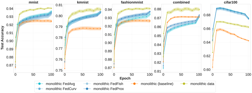
Figure 1: Mean test accuracy and standard error of the no-sharing baseline, data sharing, and federated learning with monolithic models. Sharing data is best for easier tasks while federated learning is best for harder tasks (i.e., CIFAR-100). In the heterogeneous $\mathtt{combined}$ dataset, where agents face very different tasks, aggregating models via federated methods is worse than single-agent learning.

5.2 What to share in a modular distributed setting?

Prior work [20] has noted the challenge of catastrophic forgetting that monolithic networks face in dealing with long-horizon continual problems. Modular networks [37, 36] have been proposed as a solution and have shown superior performance in maintaining task accuracy over time. We now examine the effect of different sharing modes on the DCL problem using modular networks. With the switch to modular networks, we also can now compare against partial sharing using $\mathtt{modmod}$.

Fig. 2 shows that in all datasets, partial model sharing via $\mathtt{modmod}$ consistently outperforms other methods in the initial stage of learning and provides a massive boost in learning speed. This performance is only eventually topped by $\mathtt{data}$ sharing, once enough data has been shared to characterize the tasks. This validates the claim that optimized partial parameters in the form of modules provide a significant acceleration in learning, while additional data offer strictly more information not available to the agent otherwise, leading to a higher performance eventually with sufficient training. One notable exception is the more challenging CIFAR-100 dataset where we observe that it is better to share modules than data both in terms of learning speed and final accuracy. Also, we observe that federated methods are less effective in modular networks especially in easier tasks, reaching just roughly the same performance as the isolated baseline in four datasets.

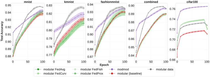
Figure 2: Mean test accuracy and standard error of the no-sharing baseline, data sharing, full-model sharing (federated learning), and partial model sharing ($\mathtt{modmod}$) with modular models. $\mathtt{modmod}$ outperforms all other methods in terms of learning speed while sharing data reaches the highest final accuracy in less difficult datasets. Federated methods are less effective in modular models; one exception is in the more difficult CIFAR-100 dataset, where it is better to share parameters than data.

5.3 How do communication constraints affect the efficacy of sharing modes?

We examine the impact of the communication constraints on the effectiveness of DCL sharing modes. We vary the number of exchanged data instances, modules, and communication frequency, and record the performance of each sharing mode. Figure 3 plots the relative gain in the final accuracy of monolithic and modular models over their respective single-agent baselines against the log of the communication expense $\log(\mathtt{B})$. The communication cost is computed as the total number of floating point numbers exchanged between a pair of agents, $\mathtt{B}=\mathtt{f}\mathtt{b}$. The frequency $\mathtt{f}$ is the number of training epochs before a communication round is initiated, so higher $\mathtt{f}$ implies less frequent communication. $\mathtt{b}$ is the number of floats exchanged per communication. See the Appendix for more details. Table 1 computes the marginal gain, which is the slope of the fitted lines in Fig. 3, and the value of the budget, which is the ratio of improvement over the communication cost $\mathtt{B}$. The result shows that partial model sharing via $\mathtt{modmod}$ is an order of magnitude more efficient than other modes.

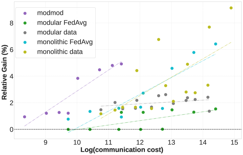
Figure 3: Relative gain in final accuracy versus the log of communication cost, $\log(\mathtt{B})$. Lines linearly fit through each sharing mode show the general trend. The results are averaged across agents, random seeds, and datasets. Qualitatively, $\mathtt{modmod}$ improves the final accuracy over isolated learning while requiring substantially less communication than other sharing modes, as further corroborated by Table 1.

	Marginal	Value of
Algorithm	Gain (%)	Budget
ModMod	1.579	$\mathbf{1.17\!\times\!10^{-4}}$
Modular Federated	0.332	$2.56\!\times\!10^{-6}$
Modular Data	0.139	$9.93\!\times\!10^{-6}$
Monolithic Federated	1.263	$1.65\!\times\!10^{-5}$
Monolithic Data	1.384	$1.13\!\times\!10^{-5}$

Table 1: Comparison of marginal gains (higher is better) and value of budget (the ratio of relative gain and communication cost; higher is better) for different sharing modes. $\mathtt{modmod}$ experiences the most favorable scaling with budget (marginal gain) and is an order of magnitude more efficient than other sharing modes (value of budget).

5.4 How does network topology affect the efficacy of sharing modes?

So far, we have only considered a fully-connected communications topology. Now we will examine the effect of network topology on the strategies’ performance. We generate Erdös–Rényi random graphs [11] with varying degrees of sparsity, and with the ring, server, and tree topologies examined in prior work [47]. As shown in Fig. 4, performance generally degrades across all sharing modes as the random graph becomes sparser. Connected topologies such as ring, server, and tree exhibit similar performance, which falls between the fully connected and the no-sharing baseline.

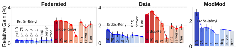
Figure 4: Relative gain in final average accuracy versus topology with modular and monolithic models. We compare four common topologies: Erdös-Rényi graphs with the probability of each edge $p\in\{1,0.75,0.5,0.3,0.1\}$, ring, server, and tree. Results are averaged across agents, random seeds, and datasets. On the vertical axis, relative gain = 0% corresponds to isolated single-agent learning with a disconnected topology ($p=0$). The results show that performance degrades as the graph becomes sparser, i.e. for low values of $p$. Ring, server, and tree have similar performance, falling between a fully connected topology ($p=1$) and the no-sharing baseline. In monolithic neural networks, the server is the worst performing among the three.

5.5 What happens when we combine all sharing modes?

The previous experiments showed that partial model ($\mathtt{modmod}$) and $\mathtt{data}$ sharing offer unique benefits, accelerating learning and improving final accuracy respectively. Here, we examine whether we can have the best of both worlds by combining all sharing modes in one hybrid approach. We compare head-to-head different modes across monolithic and modular networks both in terms of average task area under the curve (AUC) of the learning curve, and final accuracy in Table 2. The modular hybrid mode strategy consistently outperforms others in both metrics for the more challenging dataset. In easier datasets like MNIST and FashionMNIST, although the performance is more similar across strategies, those involving partial model or data sharing tend to perform best.

Table 2: Performance metrics with std. error across datasets and algorithms, including a hybrid of all sharing modes. The first number is the final average accuracy (%) and the second is average AUC.

$f$	Method	Cifar100	Combined	Fashionmnist	Kmnist	Mnist
modular	vanilla	70.04 ​$\pm$​ 0.14/71.83 ​$\pm$​ 0.13	88.58 ​$\pm$​ 0.36/88.05 ​$\pm$​ 0.28	92.80 ​$\pm$​ 0.31/92.03 ​$\pm$​ 0.32	80.63 ​$\pm$​ 0.31/80.62 ​$\pm$​ 0.31	93.47 ​$\pm$​ 0.20/92.68 ​$\pm$​ 0.22
	data	71.86 ​$\pm$​ 0.16/73.42 ​$\pm$​ 0.14	89.03 ​$\pm$​ 0.33/89.48 ​$\pm$​ 0.25	93.56 ​$\pm$​ 0.28/92.97 ​$\pm$​ 0.30	82.59 ​$\pm$​ 0.26/82.04 ​$\pm$​ 0.29	94.60 ​$\pm$​ 0.12/93.89 ​$\pm$​ 0.14
	fedavg	70.99 ​$\pm$​ 0.14/73.96 ​$\pm$​ 0.14	88.45 ​$\pm$​ 0.37/87.99 ​$\pm$​ 0.31	92.46 ​$\pm$​ 0.45/91.96 ​$\pm$​ 0.45	80.04 ​$\pm$​ 0.35/80.10 ​$\pm$​ 0.34	93.57 ​$\pm$​ 0.18/92.82 ​$\pm$​ 0.23
	fedfish	71.10 ​$\pm$​ 0.13/73.97 ​$\pm$​ 0.15	88.46 ​$\pm$​ 0.37/87.99 ​$\pm$​ 0.29	93.08 ​$\pm$​ 0.39/92.33 ​$\pm$​ 0.44	80.32 ​$\pm$​ 0.36/80.13 ​$\pm$​ 0.38	93.77 ​$\pm$​ 0.19/92.76 ​$\pm$​ 0.26
	fedcurv	71.11 ​$\pm$​ 0.13/73.94 ​$\pm$​ 0.14	88.45 ​$\pm$​ 0.37/87.99 ​$\pm$​ 0.29	93.06 ​$\pm$​ 0.40/92.32 ​$\pm$​ 0.44	80.34 ​$\pm$​ 0.36/80.14 ​$\pm$​ 0.38	93.78 ​$\pm$​ 0.19/92.76 ​$\pm$​ 0.26
	fedprox	71.82 ​$\pm$​ 0.14/73.85 ​$\pm$​ 0.13	88.47 ​$\pm$​ 0.37/88.02 ​$\pm$​ 0.29	92.93 ​$\pm$​ 0.41/92.07 ​$\pm$​ 0.46	80.48 ​$\pm$​ 0.35/80.20 ​$\pm$​ 0.35	93.93 ​$\pm$​ 0.17/93.05 ​$\pm$​ 0.21
	modmod	76.77 ​$\pm$​ 0.08/76.80 ​$\pm$​ 0.13	89.65 ​$\pm$​ 0.30/89.62 ​$\pm$​ 0.26	93.28 ​$\pm$​ 0.40/93.26 ​$\pm$​ 0.41	81.83 ​$\pm$​ 0.27/81.78 ​$\pm$​ 0.29	94.08 ​$\pm$​ 0.18/93.94 ​$\pm$​ 0.19
	hybrid	77.05 ​$\pm$​ 0.10/77.07 ​$\pm$​ 0.14	90.31 ​$\pm$​ 0.28/90.41 ​$\pm$​ 0.24	94.10 ​$\pm$​ 0.31/94.43 ​$\pm$​ 0.35	82.93 ​$\pm$​ 0.23/82.90 ​$\pm$​ 0.25	94.57 ​$\pm$​ 0.12/94.75 ​$\pm$​ 0.14
monolithic	vanilla	63.11 ​$\pm$​ 0.32/65.60 ​$\pm$​ 0.32	86.59 ​$\pm$​ 0.37/87.69 ​$\pm$​ 0.28	92.47 ​$\pm$​ 0.33/93.27 ​$\pm$​ 0.36	78.23 ​$\pm$​ 0.31/79.42 ​$\pm$​ 0.31	91.96 ​$\pm$​ 0.27/93.10 ​$\pm$​ 0.22
	data	65.18 ​$\pm$​ 0.17/67.23 ​$\pm$​ 0.21	87.82 ​$\pm$​ 0.36/88.59 ​$\pm$​ 0.28	94.02 ​$\pm$​ 0.35/94.72 ​$\pm$​ 0.38	80.70 ​$\pm$​ 0.32/81.01 ​$\pm$​ 0.29	94.20 ​$\pm$​ 0.17/94.54 ​$\pm$​ 0.21
	fedavg	67.05 ​$\pm$​ 0.16/69.11 ​$\pm$​ 0.18	86.57 ​$\pm$​ 0.40/86.76 ​$\pm$​ 0.31	93.68 ​$\pm$​ 0.39/93.60 ​$\pm$​ 0.39	80.55 ​$\pm$​ 0.33/80.49 ​$\pm$​ 0.35	93.86 ​$\pm$​ 0.20/93.76 ​$\pm$​ 0.26
	fedfish	66.85 ​$\pm$​ 0.17/68.91 ​$\pm$​ 0.17	86.55 ​$\pm$​ 0.41/86.82 ​$\pm$​ 0.31	93.64 ​$\pm$​ 0.38/93.84 ​$\pm$​ 0.40	80.39 ​$\pm$​ 0.34/80.38 ​$\pm$​ 0.36	93.65 ​$\pm$​ 0.24/93.37 ​$\pm$​ 0.31
	fedcurv	66.79 ​$\pm$​ 0.15/68.93 ​$\pm$​ 0.17	86.62 ​$\pm$​ 0.41/86.87 ​$\pm$​ 0.31	93.74 ​$\pm$​ 0.37/93.85 ​$\pm$​ 0.40	80.39 ​$\pm$​ 0.34/80.40 ​$\pm$​ 0.35	93.66 ​$\pm$​ 0.24/93.37 ​$\pm$​ 0.31
	fedprox	67.18 ​$\pm$​ 0.17/69.09 ​$\pm$​ 0.16	86.86 ​$\pm$​ 0.40/87.16 ​$\pm$​ 0.31	93.90 ​$\pm$​ 0.35/93.99 ​$\pm$​ 0.39	80.26 ​$\pm$​ 0.33/80.47 ​$\pm$​ 0.35	93.74 ​$\pm$​ 0.23/93.65 ​$\pm$​ 0.30
	hybrid	70.05 ​$\pm$​ 0.17/69.15 ​$\pm$​ 0.16	88.28 ​$\pm$​ 0.36/88.76 ​$\pm$​ 0.29	94.66 ​$\pm$​ 0.32/94.97 ​$\pm$​ 0.35	81.06 ​$\pm$​ 0.31/81.01 ​$\pm$​ 0.30	94.55 ​$\pm$​ 0.20/94.90 ​$\pm$​ 0.21

6 Conclusion

We have developed a rigorous and general definition for the DCL problem and investigated a key under-explored challenge: determining at which level to share information between agents, from the data level over partial models (modules) to full models. Our results show that partial model sharing in the form of reusable modules achieves high performance (due to reusability and flexibility) with low communications cost. When combined with data sharing in a hybrid approach, the combined modalities achieve even higher performance. By providing more competitive sharing baselines and drawing attention to the hidden cost of communication as well as assumptions on agent commonality, we address the shortcomings of earlier works and enable more robust evaluation. While our work establishes a solid bases for future DCL research, one limitation is its current focus on supervised learning. In the future, we aim to extend our work to other fields such as reinforcement learning.

Appendix A Additional Experimentation Details

Datasets

We use four common datasets MNIST, KMNIST, FashionMNIST, and CIFAR-100), following the same task sampling procedure from prior work [36] to create multiple tasks. The MNIST variants consist of 10 tasks while CIFAR has 20 tasks, where each task is a multiclass classification problem. Each agent receives different tasks drawn from the same dataset. $\mathtt{combined}$ setting is created by including tasks from MNIST, KMNIST, and FashionMNIST. In this setting, for a few (four) initial tasks, all agents receive a mixture of tasks from the three source datasets; then, they segregate into three roughly equal-sized groups, each receiving tasks drawing from exactly one source dataset. The $\mathtt{combined}$ network has 20 agents while other datasets have eight agents.

Network architectures

The agent’s models are multilayer perceptrons (MLPs) for MNIST variants and convolutional neural networks (CNNs) for CIFAR. Following prior work [36], both monolithic and modular networks start out with four modules but modular networks are allowed to dynamically add more modules.

Experimental Protocols

All experiments are repeated with eight random seeds.

Communication Budget

In the basic experiments (Sec. 5.1-5.2), each agent in data sharing is allowed $20$ queries with $5$ query neighbors every $16$ epochs while federated methods communicate every $5$ epochs, and $\mathtt{modmod}$ communicates once every task. In an extensive experiment (Sec. 5.3), we investigate the effect of varying the frequency of communication, $\mathtt{f}$, and the budget per communication, $\mathtt{b}$. For federated methods, we set $\mathtt{f}$ = 5, 10, 20, 50, 100 epochs. For $\mathtt{modmod}$, we exchange modules once per task and vary the number of sent modules (effectively $\mathtt{b}$) in 1, 2, 3, 4. For data sharing, we vary both the number of queries in $\mathtt{q}$ = 10, 20, 30 and the communication frequency in $\mathtt{f}$ = 9, 16, 50.

Sharing Algorithms

For data sharing, we use $\mathtt{Recv}$ for MNIST variants and $\mathtt{combined}$, and use $\mathtt{Simp}$ for CIFAR-100. This is because $\mathtt{Recv}$ is most effective when the sender can accurately retrieve relevant instances to a query; this is hard for CIFAR-100, so to ablate away the deficiency of the learners in $\mathtt{Recv}$ and to give data sharing a fair chance against other modes, we instead use the non-learning $\mathtt{Simp}$. For full model parameter sharing, we implement $\mathtt{FedAvg}$, $\mathtt{FedProx}$, $\mathtt{FedCurv}$, and $\mathtt{FedFish}$. As described in Sec. 4.3, modular neural networks support the dynamic addition of modules, thus agents might have different number of modules at any given time. So for federated methods, we only aggregate the basis modules—modules shared by all agents that are created during initialization [36]. The number of basis modules is set to four following the previous work. For $\mathtt{modmod}$, we use use $\mathtt{LEEP}$ metric for $\mathtt{combined}$ dataset and $\mathtt{IoU}$ for the others. $\mathtt{TrustSim}$ module selection is used in the basic experiment (Sec. 5.1-5.2) but as we get more candidate modules in the increasing budget (Sec. 5.3) we use $\mathtt{TryOut}$ instead.

Topology

Erdös–Rényi random graphs [11] with varying degrees of sparsity, and with the ring, server, and tree topologies examined in prior work [47] are used.

Compute Resources

We use Ray distributed library to parallelize agent training in a communication network. One single NVIDIA GeForce RTX 3080 takes about 10 minutes to train MNIST and $\mathtt{combined}$ datasets, and 1 hour for CIFAR-100.

Hyper-parameters

FedProx and FedCurv algorithms are run with the loss balancing factor $\mu\in\{0.001,0.01,0.1,1.0\}$, following [27, 55], and the best performing hyper-parameter for each dataset in terms of average AUC is picked for the paper.

Appendix B Budget Computation

In Sec. 5.3, we compare different sharing modes in terms of their use of $\mathtt{b}$, the number of floats exchanged per communication. We now provide more details on how $\mathtt{b}$ is computed.

For data sharing, each instance is an image, represented in memory as a tensor of size $H\cdot W\cdot C$ for height $H$, width $W$, and number of channels $C$. Then, $\mathtt{b}=H\cdot W\cdot C\cdot N$ where $N$ is the number of instances sent per communication.

For full model parameters sharing, a monolithic neural network consists of some feed-forward or convolution layers followed by a last linear layer mapping to the semantic classes. The number of parameters of a linear layer is $|W|+|b|$ for some weight matrix $W$ and bias vector $b$. The number of parameters of a convolution layer is $(c_{\textrm{in}}c_{\textrm{out}})k^{2}+c_{\textrm{out}}$ where $c_{\textrm{in}},c_{\textrm{out}}$ are in and out channels and $k$ is the kernel size. The communication cost $\mathtt{b}$ is then simply the size of the model. Although not investigated in this work, a future direction is to use model compression such as low-rank factorization [62] to have a finer-grain control over the cost of sending models in federated methods.

For modular parameter sharing, $\mathtt{b}=k\cdot M$ where $k$ is the number of shared modules, and $M$ is the module size in terms of parameters computed analogously as explained above.

Appendix C Additional Results on Hybrid Sharing

The results in this section complement those in Section 5.5. Fig. 5 shows the learning curves for the hybrid sharing, combining all sharing modes, against the other modes. It supports the results in Table 2 and shows that by combining all sharing modes in modular networks, we achieve both good initial learning and final accuracy. In monolithic networks, the hybrid mode generally outperforms others although the gain is less pronounced.

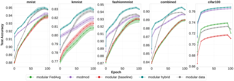
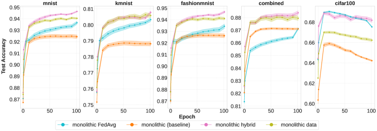
Figure 5: Mean test accuracy and standard error of a hybrid combination of all sharing modes compared against individual modes in modular (top) and monolithic (bottom) networks. In modular networks, hybrid mode achieves the best performance both in learning speed and final accuracy. The superiority of hybrid mode is less observed in monolithic networks.

The modular hybrid mode strategy consistently outperforms others in both metrics for the more challenging dataset. In easier datasets like MNIST and FashionMNIST, although the performance is more similar across strategies, those involving $\mathtt{modmod}$ or data tend to perform best.

Table 3: Relative Performance Gaps for Final and AUC Scores across Datasets. These performance gaps are reasonable proxies for task difficulties. We observe substantial improvement of DCL over single-agent learning in difficult tasks like cifar100 while the gap in performance between various strategies in easier tasks like fashionmnist is smaller.

Dataset	Final Gap (%)	AUC Gap (%)
cifar100	22.09%	17.50%
combined	4.33%	4.20%
kmnist	6.02%	4.38%
fashionmnist	1.78%	3.00%
mnist	2.87%	2.23%

References

- [1] Shai Ben-David and Reba Schuller. Exploiting task relatedness for multiple task learning. In Bernhard Schölkopf and Manfred K. Warmuth, editors, Learning Theory and Kernel Machines, pages 567–580, Berlin, Heidelberg, 2003. Springer Berlin Heidelberg.
- [2] Fei Chen and Wei Ren. On the Control of Multi-Agent Systems: A Survey. 2019.
- [3] Zhiyuan Chen and Bing Liu. Lifelong Machine Learning. Morgan & Claypool Publishers, 2nd edition, 2018.
- [4] Aakanksha Chowdhery, Sharan Narang, Jacob Devlin, Maarten Bosma, Gaurav Mishra, Adam Roberts, Paul Barham, Hyung Won Chung, Charles Sutton, Sebastian Gehrmann, Parker Schuh, Kensen Shi, Sasha Tsvyashchenko, Joshua Maynez, Abhishek Rao, Parker Barnes, Yi Tay, Noam Shazeer, Vinodkumar Prabhakaran, Emily Reif, Nan Du, Ben Hutchinson, Reiner Pope, James Bradbury, Jacob Austin, Michael Isard, Guy Gur-Ari, Pengcheng Yin, Toju Duke, Anselm Levskaya, Sanjay Ghemawat, Sunipa Dev, Henryk Michalewski, Xavier Garcia, Vedant Misra, Kevin Robinson, Liam Fedus, Denny Zhou, Daphne Ippolito, David Luan, Hyeontaek Lim, Barret Zoph, Alexander Spiridonov, Ryan Sepassi, David Dohan, Shivani Agrawal, Mark Omernick, Andrew M. Dai, Thanumalayan Sankaranarayana Pillai, Marie Pellat, Aitor Lewkowycz, Erica Moreira, Rewon Child, Oleksandr Polozov, Katherine Lee, Zongwei Zhou, Xuezhi Wang, Brennan Saeta, Mark Diaz, Orhan Firat, Michele Catasta, Jason Wei, Kathy Meier-Hellstern, Douglas Eck, Jeff Dean, Slav Petrov, and Noah Fiedel. Palm: Scaling language modeling with pathways, 2022.
- [5] Embodiment Collaboration, Abby O’Neill, Abdul Rehman, Abhiram Maddukuri, Abhishek Gupta, Abhishek Padalkar, Abraham Lee, Acorn Pooley, Agrim Gupta, Ajay Mandlekar, Ajinkya Jain, Albert Tung, Alex Bewley, Alex Herzog, Alex Irpan, Alexander Khazatsky, Anant Rai, Anchit Gupta, Andrew Wang, Anikait Singh, Animesh Garg, Aniruddha Kembhavi, Annie Xie, Anthony Brohan, Antonin Raffin, Archit Sharma, Arefeh Yavary, Arhan Jain, Ashwin Balakrishna, Ayzaan Wahid, Ben Burgess-Limerick, Beomjoon Kim, Bernhard Schölkopf, Blake Wulfe, Brian Ichter, Cewu Lu, Charles Xu, Charlotte Le, Chelsea Finn, Chen Wang, Chenfeng Xu, Cheng Chi, Chenguang Huang, Christine Chan, Christopher Agia, Chuer Pan, Chuyuan Fu, Coline Devin, Danfei Xu, Daniel Morton, Danny Driess, Daphne Chen, Deepak Pathak, Dhruv Shah, Dieter Büchler, Dinesh Jayaraman, Dmitry Kalashnikov, Dorsa Sadigh, Edward Johns, Ethan Foster, Fangchen Liu, Federico Ceola, Fei Xia, Feiyu Zhao, Freek Stulp, Gaoyue Zhou, Gaurav S. Sukhatme, Gautam Salhotra, Ge Yan, Gilbert Feng, Giulio Schiavi, Glen Berseth, Gregory Kahn, Guanzhi Wang, Hao Su, Hao-Shu Fang, Haochen Shi, Henghui Bao, Heni Ben Amor, Henrik I Christensen, Hiroki Furuta, Homer Walke, Hongjie Fang, Huy Ha, Igor Mordatch, Ilija Radosavovic, Isabel Leal, Jacky Liang, Jad Abou-Chakra, Jaehyung Kim, Jaimyn Drake, Jan Peters, Jan Schneider, Jasmine Hsu, Jeannette Bohg, Jeffrey Bingham, Jeffrey Wu, Jensen Gao, Jiaheng Hu, Jiajun Wu, Jialin Wu, Jiankai Sun, Jianlan Luo, Jiayuan Gu, Jie Tan, Jihoon Oh, Jimmy Wu, Jingpei Lu, Jingyun Yang, Jitendra Malik, João Silvério, Joey Hejna, Jonathan Booher, Jonathan Tompson, Jonathan Yang, Jordi Salvador, Joseph J. Lim, Junhyek Han, Kaiyuan Wang, Kanishka Rao, Karl Pertsch, Karol Hausman, Keegan Go, Keerthana Gopalakrishnan, Ken Goldberg, Kendra Byrne, Kenneth Oslund, Kento Kawaharazuka, Kevin Black, Kevin Lin, Kevin Zhang, Kiana Ehsani, Kiran Lekkala, Kirsty Ellis, Krishan Rana, Krishnan Srinivasan, Kuan Fang, Kunal Pratap Singh, Kuo-Hao Zeng, Kyle Hatch, Kyle Hsu, Laurent Itti, Lawrence Yunliang Chen, Lerrel Pinto, Li Fei-Fei, Liam Tan, Linxi "Jim" Fan, Lionel Ott, Lisa Lee, Luca Weihs, Magnum Chen, Marion Lepert, Marius Memmel, Masayoshi Tomizuka, Masha Itkina, Mateo Guaman Castro, Max Spero, Maximilian Du, Michael Ahn, Michael C. Yip, Mingtong Zhang, Mingyu Ding, Minho Heo, Mohan Kumar Srirama, Mohit Sharma, Moo Jin Kim, Naoaki Kanazawa, Nicklas Hansen, Nicolas Heess, Nikhil J Joshi, Niko Suenderhauf, Ning Liu, Norman Di Palo, Nur Muhammad Mahi Shafiullah, Oier Mees, Oliver Kroemer, Osbert Bastani, Pannag R Sanketi, Patrick "Tree" Miller, Patrick Yin, Paul Wohlhart, Peng Xu, Peter David Fagan, Peter Mitrano, Pierre Sermanet, Pieter Abbeel, Priya Sundaresan, Qiuyu Chen, Quan Vuong, Rafael Rafailov, Ran Tian, Ria Doshi, Roberto Martín-Martín, Rohan Baijal, Rosario Scalise, Rose Hendrix, Roy Lin, Runjia Qian, Ruohan Zhang, Russell Mendonca, Rutav Shah, Ryan Hoque, Ryan Julian, Samuel Bustamante, Sean Kirmani, Sergey Levine, Shan Lin, Sherry Moore, Shikhar Bahl, Shivin Dass, Shubham Sonawani, Shuran Song, Sichun Xu, Siddhant Haldar, Siddharth Karamcheti, Simeon Adebola, Simon Guist, Soroush Nasiriany, Stefan Schaal, Stefan Welker, Stephen Tian, Subramanian Ramamoorthy, Sudeep Dasari, Suneel Belkhale, Sungjae Park, Suraj Nair, Suvir Mirchandani, Takayuki Osa, Tanmay Gupta, Tatsuya Harada, Tatsuya Matsushima, Ted Xiao, Thomas Kollar, Tianhe Yu, Tianli Ding, Todor Davchev, Tony Z. Zhao, Travis Armstrong, Trevor Darrell, Trinity Chung, Vidhi Jain, Vincent Vanhoucke, Wei Zhan, Wenxuan Zhou, Wolfram Burgard, Xi Chen, Xiaolong Wang, Xinghao Zhu, Xinyang Geng, Xiyuan Liu, Xu Liangwei, Xuanlin Li, Yao Lu, Yecheng Jason Ma, Yejin Kim, Yevgen Chebotar, Yifan Zhou, Yifeng Zhu, Yilin Wu, Ying Xu, Yixuan Wang, Yonatan Bisk, Yoonyoung Cho, Youngwoon Lee, Yuchen Cui, Yue Cao, Yueh-Hua Wu, Yujin Tang, Yuke Zhu, Yunchu Zhang, Yunfan Jiang, Yunshuang Li, Yunzhu Li, Yusuke Iwasawa, Yutaka Matsuo, Zehan Ma, Zhuo Xu, Zichen Jeff Cui, Zichen Zhang, Zipeng Fu, and Zipeng Lin. Open x-embodiment: Robotic learning datasets and rt-x models, 2024.
- [6] G. Csibra and G. Gergely. Natural pedagogy as evolutionary adaptation. Philos Trans R Soc Lond B Biol Sci, 366(1567):1149–1157, Apr 2011.
- [7] I. Csiszar. -Divergence Geometry of Probability Distributions and Minimization Problems. The Annals of Probability, 3(1):146 – 158, 1975.
- [8] Mathijs de Weerdt and Brad Clement. Introduction to planning in multiagent systems. Multiagent and Grid Systems, 5:345–355, 2009. 4.
- [9] Ali Dorri, Salil S. Kanhere, and Raja Jurdak. Multi-agent systems: A survey. IEEE Access, 6:28573–28593, 2018.
- [10] Edmund H. Durfee. Distributed Problem Solving and Planning, pages 118–149. Springer Berlin Heidelberg, Berlin, Heidelberg, 2001.
- [11] P Erdös and A Rényi. On random graphs i. Publicationes Mathematicae Debrecen, 6:290–297, 1959.
- [12] Melinda Fagan. Collective scientific knowledge. Philosophy Compass, 7(12):821–831, 2012.
- [13] William Fedus, Barret Zoph, and Noam Shazeer. Switch transformers: Scaling to trillion parameter models with simple and efficient sparsity, 2022.
- [14] Jakob Foerster, Gregory Farquhar, Triantafyllos Afouras, Nantas Nardelli, and Shimon Whiteson. Counterfactual multi-agent policy gradients, 2017.
- [15] Yunhao Ge, Yuecheng Li, Di Wu, Ao Xu, Adam M. Jones, Amanda Sofie Rios, Iordanis Fostiropoulos, shixian wen, Po-Hsuan Huang, Zachary William Murdock, Gozde Sahin, Shuo Ni, Kiran Lekkala, Sumedh Anand Sontakke, and Laurent Itti. Lightweight learner for shared knowledge lifelong learning. Transactions on Machine Learning Research, 2023.
- [16] Yuchong Geng, Dongyue Zhang, Po-han Li, Oguzhan Akcin, Ao Tang, and Sandeep P. Chinchali. Decentralized sharing and valuation of fleet robotic data. In Aleksandra Faust, David Hsu, and Gerhard Neumann, editors, Proceedings of the 5th Conference on Robot Learning, volume 164 of Proceedings of Machine Learning Research, pages 1795–1800. PMLR, 08–11 Nov 2022.
- [17] David Isele and Akansel Cosgun. Selective experience replay for lifelong learning. In AAAI, 2018.
- [18] Sangwon Jung, Hongjoon Ahn, Sungmin Cha, and Taesup Moon. Adaptive group sparse regularization for continual learning. NeurIPS, 2020.
- [19] Daniel Kifer, Shai Ben-David, and Johannes Gehrke. Detecting change in data streams. pages 180–191, 04 2004.
- [20] James Kirkpatrick, Razvan Pascanu, Neil Rabinowitz, Joel Veness, Guillaume Desjardins, Andrei A. Rusu, Kieran Milan, John Quan, Tiago Ramalho, Agnieszka Grabska-Barwinska, Demis Hassabis, Claudia Clopath, Dharshan Kumaran, and Raia Hadsell. Overcoming catastrophic forgetting in neural networks. Proceedings of the National Academy of Sciences, 114(13):3521–3526, mar 2017.
- [21] Louis Kirsch, Julius Kunze, and David Barber. Modular networks: Learning to decompose neural computation, 2018.
- [22] Long Le, Dana Hughes, and Katia Sycara. Multi-agent hierarchical reinforcement learning in urban and search rescue. Robotics Institute Summer Scholar’ Working Papers Journals, 9:157–164, 2021.
- [23] Seungwon Lee, James Stokes, and Eric Eaton. Learning shared knowledge for deep lifelong learning using deconvolutional networks. In Proceedings of the Twenty-Eighth International Joint Conference on Artificial Intelligence, IJCAI-19, pages 2837–2844. International Joint Conferences on Artificial Intelligence Organization, 7 2019.
- [24] Sergey Levine, Peter Pastor, Alex Krizhevsky, and Deirdre Quillen. Learning hand-eye coordination for robotic grasping with deep learning and large-scale data collection, 2016.
- [25] Huao Li, Long Le, Max Chis, Keyang Zheng, Dana Hughes, Michael Lewis, and Katia Sycara. Sequential theory of mind modeling in team search and rescue tasks. In Nikolos Gurney and Gita Sukthankar, editors, Computational Theory of Mind for Human-Machine Teams, pages 158–172, Cham, 2022. Springer Nature Switzerland.
- [26] Tian Li, Anit Kumar Sahu, Ameet Talwalkar, and Virginia Smith. Federated learning: Challenges, methods, and future directions. IEEE Signal Processing Magazine, 37(3):50–60, may 2020.
- [27] Tian Li, Anit Kumar Sahu, Manzil Zaheer, Maziar Sanjabi, Ameet Talwalkar, and Virginia Smith. Federated optimization in heterogeneous networks, 2020.
- [28] Xiaoxiao Li, Meirui Jiang, Xiaofei Zhang, Michael Kamp, and Qi Dou. Fedbn: Federated learning on non-iid features via local batch normalization, 2021.
- [29] Zhizhong Li and Derek Hoiem. Learning without forgetting, 2017.
- [30] Kuo-Yun Liang, Abhishek Srinivasan, and Juan Carlos Andresen. Modular federated learning. In 2022 International Joint Conference on Neural Networks (IJCNN). IEEE, jul 2022.
- [31] David Lopez-Paz and Marc’Aurelio Ranzato. Gradient episodic memory for continual learning, 2022.
- [32] Zichen Ma, Yu Lu, Zihan Lu, Wenye Li, Jinfeng Yi, and Shuguang Cui. Towards heterogeneous clients with elastic federated learning, 2021.
- [33] Yishay Mansour, Mehryar Mohri, and Afshin Rostamizadeh. Domain adaptation: Learning bounds and algorithms, 2023.
- [34] Michael McCloskey and Neal J. Cohen. Catastrophic interference in connectionist networks: The sequential learning problem. volume 24 of Psychology of Learning and Motivation, pages 109–165. Academic Press, 1989.
- [35] H. Brendan McMahan, Eider Moore, Daniel Ramage, Seth Hampson, and Blaise Agüera y Arcas. Communication-efficient learning of deep networks from decentralized data, 2023.
- [36] Jorge A. Mendez and Eric Eaton. Lifelong learning of compositional structures, 2021.
- [37] Jorge A. Mendez and Eric Eaton. How to reuse and compose knowledge for a lifetime of tasks: A survey on continual learning and functional composition, 2023.
- [38] Jorge A. Mendez, Marcel Hussing, Meghna Gummadi, and Eric Eaton. Composuite: A compositional reinforcement learning benchmark, 2022.
- [39] Jorge A. Mendez, Harm van Seijen, and Eric Eaton. Modular lifelong reinforcement learning via neural composition, 2022.
- [40] Elliot Meyerson and Risto Miikkulainen. Beyond shared hierarchies: Deep multitask learning through soft layer ordering, 2018.
- [41] Javad Mohammadi and Soheil Kolouri. Collaborative learning through shared collective knowledge and local expertise. In 2019 IEEE 29th International Workshop on Machine Learning for Signal Processing (MLSP), pages 1–6, 2019.
- [42] Saptarshi Nath, Christos Peridis, Eseoghene Ben-Iwhiwhu, Xinran Liu, Shirin Dora, Cong Liu, Soheil Kolouri, and Andrea Soltoggio. Sharing lifelong reinforcement learning knowledge via modulating masks, 2023.
- [43] Cuong V. Nguyen, Tal Hassner, Matthias Seeger, and Cedric Archambeau. Leep: A new measure to evaluate transferability of learned representations, 2020.
- [44] German I. Parisi, Ronald Kemker, Jose L. Part, Christopher Kanan, and Stefan Wermter. Continual lifelong learning with neural networks: A review. Neural Networks, 113:54–71, 2019.
- [45] Benedetto Piccoli. Control of multi-agent systems: results, open problems, and applications, 2023.
- [46] Anthony Robins. Catastrophic forgetting, rehearsal and pseudorehearsal. Connection Science, 7(2):123–146, 1995.
- [47] Mohammad Rostami, Soheil Kolouri, Kyungnam Kim, and Eric Eaton. Multi-agent distributed lifelong learning for collective knowledge acquisition, 2018.
- [48] Daniel Rothchild, Ashwinee Panda, Enayat Ullah, Nikita Ivkin, Ion Stoica, Vladimir Braverman, Joseph Gonzalez, and Raman Arora. Fetchsgd: Communication-efficient federated learning with sketching, 2020.
- [49] Andrei A. Rusu, Neil C. Rabinowitz, Guillaume Desjardins, Hubert Soyer, James Kirkpatrick, Koray Kavukcuoglu, Razvan Pascanu, and Raia Hadsell. Progressive neural networks, 2022.
- [50] Paul Ruvolo and Eric Eaton. ELLA: An efficient lifelong learning algorithm. In Sanjoy Dasgupta and David McAllester, editors, Proceedings of the 30th International Conference on Machine Learning, volume 28 of Proceedings of Machine Learning Research, pages 507–515, Atlanta, Georgia, USA, 17–19 Jun 2013. PMLR.
- [51] Jonathan Schwarz, Jelena Luketina, Wojciech M. Czarnecki, Agnieszka Grabska-Barwinska, Yee Whye Teh, Razvan Pascanu, and Raia Hadsell. Progress & compress: A scalable framework for continual learning, 2018.
- [52] E. Semsar-Kazerooni and K. Khorasani. A game theory approach to multi-agent team cooperation. In 2009 American Control Conference, pages 4512–4518, 2009.
- [53] Burr Settles. Active learning literature survey. Computer Sciences Technical Report 1648, University of Wisconsin–Madison, 2009.
- [54] Donald Shenaj, Marco Toldo, Alberto Rigon, and Pietro Zanuttigh. Asynchronous federated continual learning, 2023.
- [55] Neta Shoham, Tomer Avidor, Aviv Keren, Nadav Israel, Daniel Benditkis, Liron Mor-Yosef, and Itai Zeitak. Overcoming forgetting in federated learning on non-iid data, 2019.
- [56] Andrea Soltoggio, Eseoghene Ben-Iwhiwhu, Vladimir Braverman, Eric Eaton, Benjamin Epstein, Yunhao Ge, Lucy Halperin, Jonathan How, Laurent Itti, Michael A. Jacobs, Pavan Kantharaju, Long Le, Steven Lee, Xinran Liu, Sildomar T. Monteiro, David Musliner, Saptarshi Nath, Priyadarshini Panda, Christos Peridis, Hamed Pirsiavash, Vishwa Parekh, Kaushik Roy, Shahaf Shperberg, Hava T. Siegelmann, Peter Stone, Kyle Vedder, Jingfeng Wu, Lin Yang, Guangyao Zheng, and Soheil Kolouri. A collective ai via lifelong learning and sharing at the edge. Nature Machine Intelligence, 6(3):251–264, Mar 2024.
- [57] Sebastian U. Stich. Local sgd converges fast and communicates little, 2019.
- [58] Peter Stone and Manuela Veloso. Multiagent systems: A survey from a machine learning perspective. Autonomous Robots, 8(3):345–383, Jun 2000.
- [59] Tao Sun, Dongsheng Li, and Bao Wang. Decentralized federated averaging, 2021.
- [60] Yang Tan, Yang Li, and Shao-Lun Huang. Otce: A transferability metric for cross-domain cross-task representations. In Proceedings of the IEEE/CVF Conference on Computer Vision and Pattern Recognition (CVPR), pages 15779–15788, June 2021.
- [61] Gido M. van de Ven and Andreas S. Tolias. Three scenarios for continual learning. CoRR, abs/1904.07734, 2019.
- [62] Thijs Vogels, Sai Praneeth Karimireddy, and Martin Jaggi. Powergossip: Practical low-rank communication compression in decentralized deep learning, 2020.
- [63] Tianchun Wang, Wei Cheng, Dongsheng Luo, Wenchao Yu, Jingchao Ni, Liang Tong, Haifeng Chen, and Xiang Zhang. Personalized federated learning via heterogeneous modular networks, 2022.
- [64] Jaehong Yoon, Wonyong Jeong, Giwoong Lee, Eunho Yang, and Sung Ju Hwang. Federated continual learning with weighted inter-client transfer, 2021.
- [65] Jaehong Yoon, Saehoon Kim, Eunho Yang, and Sung Ju Hwang. Scalable and order-robust continual learning with additive parameter decomposition, 2020.
- [66] Jaehong Yoon, Eunho Yang, Jeongtae Lee, and Sung Ju Hwang. Lifelong learning with dynamically expandable networks, 2018.
- [67] Friedemann Zenke, Ben Poole, and Surya Ganguli. Continual learning through synaptic intelligence, 2017.
Technical Appendices for “Distributed Continual Learning”