Data Valuation by Leveraging Global and
Local Statistical Information

Abstract

Data valuation has garnered increasing attention in recent years, given the critical role of high-quality data in various applications, particularly in machine learning tasks. There are diverse technical avenues to quantify the value of data within a corpus. While Shapley value-based methods are among the most widely used techniques in the literature due to their solid theoretical foundation, the accurate calculation of Shapley values is often intractable, leading to the proposal of numerous approximated calculation methods. Despite significant progress, nearly all existing methods overlook the utilization of distribution information of values within a data corpus. In this paper, we demonstrate that both global and local statistical information of value distributions hold significant potential for data valuation within the context of machine learning. Firstly, we explore the characteristics of both global and local value distributions across several simulated and real data corpora. Useful observations and clues are obtained. Secondly, we propose a new data valuation method that estimates Shapley values by incorporating the explored distribution characteristics into an existing method, AME. Thirdly, we present a new path to address the dynamic data valuation problem by formulating an optimization problem that integrates information of both global and local value distributions. Extensive experiments are conducted on Shapley value estimation, value-based data removal/adding, mislabeled data detection, and incremental/decremental data valuation. The results showcase the effectiveness and efficiency of our proposed methodologies, affirming the significant potential of global and local value distributions in data valuation.

I Introduction

Data valuation aims to quantify the value of a datum in a dataset for business, scientific discovery, and applications such as classifier training [1, 2, 3]. It is a new yet hot research topic in data-centric research communities and industrial areas, as a dataset with a large proportion of highly valuable data quite benefits real use. It is also a basis for data pricing in data economics [4]. Therefore, the construction of an effective data valuation method is of great importance for data-centric applications and transactions. Existing data valuation methods can be divided into four folds [5]: marginal contribution-based [6, 7], gradient-based [8, 9], importance weight-based [10], and out-of-bag estimation-based [11] methods. Among the four technical approaches, the marginal contribution-based technique stands out as the most popular and consistently delivers strong performance. It utilizes the average utility change when a certain datum is removed from a set with a given cardinality to characterize the datum’s value.

An important index, namely, Shapley value which is a key concept in cooperative game [12, 13], is usually used to calculate the marginal contribution for data valuation. Due to its solid theoretical basis, Shapley value is among the primary choices in data valuation [14, 15, 16, 6]. However, the accurate calculation of the Shapley value for a given data corpus is nearly intractable as the computational complexity is about $O(2^{N})$ for $N$ samples. Therefore, researchers have made efforts toward the approximate yet efficient valuation methodology. For example, Jia et al. [17] investigated the scenario when data are used for training a KNN classifier and proposed a novel efficient method, KNN Shapley, exactly in $O(N\log N)$ time.

A recent study assumes a sparse assumption for the values of data to reduce the computational load of an approximate method, namely, average marginal estimation (AME) [7]. The theoretical analysis indicates that the estimated AME scores are asymptotically converged to the true Shapley values. Although promising results are obtained, we argue that the potential of value distribution in data valuation is overwhelmingly ignored in almost all previous studies. The sparse assumption utilized in AME actually presumes that the data values in a dataset conform to the Laplace distribution (detailed in Section II-B). However, our findings indicate that this assumption may not always be justified. The value distribution in this study consists of two parts: local distribution which captures the relationship between a datum and its neighborhood, and global value distribution for all involved data. Through our experimental exploration, we have verified that compared with the Laplace distribution, the distribution of data values in a dataset is closer to a Gaussian distribution. Furthermore, we have observed that the values of close samples (samples in the same neighborhood) are tightly correlated. Specifically, the similarities in values between neighboring data points within the same category are substantial, whereas the similarities in values between neighboring data points from different categories are minimal.

Another inspiration for this study is dynamic data valuation, which requires quantifying the data values when a group of new data is added or a batch of original data is deleted. To the best of our knowledge, there is only one study referring to dynamic data valuation, which is conducted by Zhang et al. [18]. This pioneering study transforms the conventional calculation for Shapley value into an incremental paradigm. When adding a new datum, about half of the computational cost can be saved. Illuminated by our observations mentioned above, the value of a single datum can be inferred based on its neighborhood. This intuitive observation inspires us to explore an alternative way to deal with dynamic data valuation.

This study attempts to explore the global and local distribution characteristics of the values for a dataset and investigate how to apply them to both conventional and dynamic data valuation. Firstly, both synthetic and real datasets are leveraged to make statistical analyses for the characteristics of both global and local value distributions. Useful observations and clues are obtained on the basis of the statistical results and the discussion of previous methods. Secondly, two new methods for data valuation are proposed. Specifically, the first method applies the distribution characteristics to one classical Shapley value-based data valuation method, namely, AME [7]. Theoretically, many existing methods can replace AME in our method. The second approach constructs a new optimization problem integrating distribution characteristics for dynamic data valuation. Corresponding algorithms are proposed to solve the optimization problem. Thirdly, extensive experiments are performed on various benchmark datasets to assess the effectiveness of our methodologies across diverse tasks.

Experimental results on Shapley value estimation show that compared to AME, our estimated data values are closer to the true Shapley values. Experimental results on value-based point adding and removing tasks verify the ability of our approach to identify influential and poisoned samples. Moreover, our approach achieves competitive performance on mislabeled data detection tasks compared with other Shapley value-based valuation methods. Furthermore, our proposed dynamic data valuation approaches consistently achieve state-of-the-art performance, as well as substantially enhancing calculation efficiency.

Overall, our main contributions can be summarized as follows:

• The characteristics of global and local distributions of data values on a data corpus are explored and applied to data valuation. To our knowledge, this is the first work that focuses on the investigation of value distribution information in data valuation.

• A new data valuation method is proposed by integrating global and local distribution information into regularizers, which can easily be combined with many existing data valuation methods.

• Two new dynamic data valuation methods are proposed to solve the incremental and decremental valuations, respectively. These methods construct a mathematical optimization problem based on the value distribution information. Corresponding algorithms are designed to solve the optimization problem.

• Extensive experiments are performed on various benchmark datasets to validate the effectiveness of the proposed methodologies, which support the great potential of information from value distribution in data valuation.

II Related Work

II-A Data Valuation

High-quality data are valuable for many real-world applications [19, 20]. Nevertheless, real-world data usually exhibit heterogeneity and noise [21, 22]. Therefore, the accurate quantification of the value of each datum in a dataset is of great importance for the involved applications and the data transactions in the data market. As introduced in Section I, existing data valuation methods can be divided into the following four folds:

• Marginal contribution-based methods: This kind of methods calculates the differences of the utility with or without the datum to be quantified. The larger the utility difference is, the more valuable the datum is. Representative methods include leave-one-out (LOO) [5], Data Banzhaf [23], and a series of Sharpley value-based methods such as Data Shapley [16], Beta Shapley [6], and AME [7].

• Gradient-based methods: This kind of methods calculates the change of the utility value when the weight of the datum to be quantified is increased. Two representative methods are Influence function [24] and LAVA [9].

• Importance weight-based methods: This kind of methods learns an important weight for a datum to be quantified during training and takes the weight as the value. Naturally, importance weight-based methods are particularly proposed for machine learning applications. One representative method is DVRL [10], which utilizes the reinforcement learning technique to learn sample weights.

• Out-of-bag estimation-based methods: This kind of methods is also designed particularly for machine learning tasks. The representative method, Data-OOB [11], calculates the contribution of each data point using out-of-bag accuracy when a bagging model (e.g., random forest) is employed.

Additionally, Jiang et al. [5] developed a standardized benchmarking system for data valuation. They summarized four downstream machine learning tasks for evaluating the values estimated by different data valuation methods. Their results suggest that no single algorithm performs uniformly best across all tasks. Zhang et al. [18] proposed an efficient updating method when dynamically adding/deleting data points. Three concrete algorithms are proposed in their study and the entire computation cost is reduced to some extent compared with other previous Shapley value-based methods. Nevertheless, existing algorithms are still constrained by suboptimal efficiency and performance.

II-B Distribution-Aided Learning

In machine learning, a large number of learning methods investigate the utilization of distribution information in model training [25]. There are two representative learning methods, namely, LASSO [26] and ridge regression, which considers the prior distribution of model parameters in regression. Take LASSO as an example, it learns the model by solving the following problem:

$$\underset{\boldsymbol{\omega}}{\min}\sum_{\boldsymbol{x}}||y-\boldsymbol{\omega}^{T}\boldsymbol{x}||_{2}^{2}+\lambda||\boldsymbol{\omega}||_{1},$$ (1)

where $\boldsymbol{\omega}$ is the model parameter, $\boldsymbol{x}$ is a sample, $y$ is the target, and $\lambda$ is a hyperparameter that controls the strength of the regularization. LASSO can be inferred from a statistical view. Assuming that the prior distribution $\boldsymbol{\omega}$ conforms to a Laplace distribution as follows:

$$\boldsymbol{\omega}\sim\dfrac{1}{2\sigma}e^{-\dfrac{||\boldsymbol{\omega}||_{1}}{\sigma}},$$ (2)

where $\sigma$ is a parameter. When the maximum a posteriori estimation is applied, we obtain

$$\boldsymbol{\omega}^{*} =\arg\underset{\boldsymbol{\omega}}{\max}\ln[\prod_{\boldsymbol{x}}\dfrac{1}{\sqrt{2\pi}\sigma_{1}}e^{\dfrac{-||y-\boldsymbol{\omega}^{T}\boldsymbol{x}||_{2}^{2}}{2\sigma_{1}^{2}}}\cdot\dfrac{1}{\sigma_{2}}e^{-\dfrac{||\boldsymbol{\omega}||_{1}}{\sigma_{2}}}]$$ (3)

$$\sim\arg\underset{\boldsymbol{\omega}}{\min}||y-\boldsymbol{\omega}^{T}\boldsymbol{x}||_{2}^{2}+\frac{2\sigma_{1}^{2}}{\sigma_{2}}||\boldsymbol{\omega}||_{1},$$

where the coefficient ${2\sigma_{1}^{2}}/{\sigma_{2}}$ can be reduced to a single hyperparameter $\lambda$. The loss in Eq. (3) is exactly the loss in LASSO. If the distribution in Eq. (2) is replaced by the Gaussian distribution, then ridge regression can also be obtained. Additionally, in multi-task learning, the distribution of the model parameters is also utilized to connect the multiple tasks. A widely used regularizer [27] is $\sum_{t}||\boldsymbol{\omega}_{t}-\boldsymbol{\bar{\omega}}||_{2}^{2}$, where $\boldsymbol{\omega}_{t}$ is the model parameter of the $t$th task and $\boldsymbol{\bar{\omega}}$ is the mean of the model parameters. This underlying assumption for this regularizer is that $\boldsymbol{\omega}_{t}$ conforms to a Gaussian distribution with the mean $\boldsymbol{\bar{\omega}}$.

Local distribution information is also prevailing in many machine learning tasks. Most local distribution information refers to the high similarity between samples that are close to each other. For example, samples in the neighborhood usually share the same labels in statistics. Therefore, a well-known yet effective classifier, namely, KNN [28], is developed. Zhu et al. [29] designed a new linear discriminative analysis method to seek the projected directions which makes sure that the within-neighborhood scatter is as small as possible and the between-neighborhood scatter is as large as possible. Furthermore, Zhong et al. [30] revealed that a DNN trained on the supervised data generates representations in which a generic query sample and its neighbors usually share the same label. So far, local distribution information has not been applied in the data valuation field.

III Empirical Exploration

In this section, we conduct analytical experiments on both simulated and real datasets to investigate the properties of global and local distributions of data values, and the value variations when new data are added or existing data are removed. The common notations in this paper are summarized in Table I.

First, we introduce our three employed datasets:

• Random: This simulated dataset is randomly sampled from the following data distribution:

  $$y\stackrel{{\scriptstyle u.a.r}}{{\sim}}\{-1,+1\},\quad\boldsymbol{\theta}=[{+1,+1}]^{T}\in\mathbb{R}^{2},$$ (4)

  $$\boldsymbol{x}\sim\left\{\begin{array}[]{ll}\mathcal{N}\left(\boldsymbol{\theta},\sigma_{+}^{2}\boldsymbol{I}\right),&\text{ if }y=+1\\ \mathcal{N}\left(-\boldsymbol{\theta},\sigma_{-}^{2}\boldsymbol{I}\right),&\text{ if }y=-1\end{array}\right.,$$

  where $\mathcal{N}(\cdot,\cdot)$ is a Gaussian distribution, with the mean $\boldsymbol{\theta}$. $\boldsymbol{I}$ refers to the identity matrix. A $K$-factor difference is set between two classes’ variances, that is $\sigma_{+}\!:\!\sigma_{-}\!=\!K\!:\!1$ and $K\!=\!2$. Moreover, $\sigma_{-}\!=\!1$. There are 5,000 sampled data in the training set and the test set for both categories +1 and -1 respectively.

• electricity: This dataset is real-world tabular corpus [31]. It consists of 38,474 training samples in two classes. Each sample is represented by six-dimensional features.

• CIFAR10-embeddings: This dataset is real-world image corpus [32]. Its training data consists of 50,000 samples in ten classes. Each image is represented by 2,048-dimensional deep features.

III-A Analysis for Global and Local Value Distributions

This section analyzes the global and local value distributions of samples. The Shapely value of training data is considered the true value. We utilize the AME method [7] to estimate the Shapely values as its estimated scores can asymptotically converge to the true Shapley values when the number of sampled subsets becomes large. In our experiments, the number of sampled subsets for each dataset is set as the number of all samples. In this setting, the sparsity assumption is not required and thus the Mean Square Error (MSE)-based estimation in AME can be used rather than its LASSO-based approximation. Two statistical analyses are performed for the estimated values on the three datasets. The first is about the distribution of the values of all involved samples in each dataset; the second is about the difference between the values of a sample and its closest neighbor.

TABLE I: Summary of notations.

Notation	Description
$\boldsymbol{x}$	a datum
$y$	a categorical label
$N$	the size of a training set
$\boldsymbol{\beta}$	the vector of the values in a dataset
$\boldsymbol{U}$	the vector of utilities
$S_{i,j}$	the similarity between the values of samples $\boldsymbol{x}_{i}$ and $\boldsymbol{x}_{j}$
$\mathcal{N}_{k}(\boldsymbol{x}_{i})$	the index set of data in the $k$-neighborhood of $\boldsymbol{x}_{i}$
$r_{\mathcal{N}_{k}}(\boldsymbol{x}_{i})$	the neighborhood variation of $\boldsymbol{x}_{i}$
$\boldsymbol{I}$	the unit matrix
$\mathcal{D}$	the training dataset
$\mathcal{D}^{\prime}$	the added or deleted dataset
$\mathbb{R}^{n}$	the $n$-dimensional Euclid space
$\mathbb{I}(\cdot)$	the indicator function
$\mathcal{N}(\cdot,\cdot)$	a Gaussian distribution

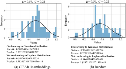
Figure 1: Histograms of data values after min-max normalization for two datasets, including CIFAR10-embeddings (a) and Random (b) datasets.

In the first statistical analysis, we depict the distributions of values on two datasets, including CIFAR10-embeddings and Random. The results are illustrated in Fig. 1. Although these distributions in Fig. 1 look like Gaussian or Laplace distributions, the hypothesis tests we performed gave different conclusions. We take the predicted probability of each sample in the test set as the query, and then we perform the KStest hypothesis testing method [33]. The results of the hypothesis testing method KStest, as illustrated below the graph, show that the value distribution of these two datasets conforms to the Gaussian distribution but does not conform to the Laplace distribution. These findings indicate that compared to the Laplace distribution, the value distribution is more in line with the Gaussian distribution. AME claimed that the distribution of values is a Laplace distribution, but the results of our statistical analysis do not support it. This means that the distribution of data values has yet to be explored in detail.

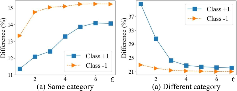
Figure 2: (a): The average relative difference between the value of a sample and the values of its neighbors from the same category. (b): The average relative difference between the value of a sample and the values of its neighbors with different class labels. $\epsilon$ is the range of the neighborhood.

In the second statistical analysis, two types of differences are considered. The first type concerns the relative difference between a datum and its neighbors in the same category; the second type concerns the relative difference between the values of a single sample and its neighbors from a different category. Fig. 2(a) depicts the relative difference between a datum and its neighbors with the same label for both two classes +1 and -1 respectively. With the neighborhood range $\epsilon$ increasing, the relative difference also becomes larger, that is, the value of a single sample is close to the value of its neighboring samples from the same category, and the closer the distance, the closer their values are. Moreover, Fig. 2(b) illustrates the relative difference between the value of a single sample and the values of its neighbors with different class labels. As the neighborhood size $\epsilon$ becomes larger, the relative difference becomes smaller. This finding reveals that the sample values are not close to the values of its neighboring samples from different categories, and the closer the distance, the greater the relative value difference.

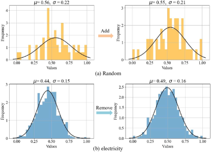
Figure 3: Normalized value variation after adding (a) and removing data points (b) on electricity and Random datasets.

III-B Analysis for Value Variations

Two additional statistical analyses are conducted to investigate variations in values resulting from the addition of new data and the removal of existing data, respectively. In the first analysis, 90% of the samples from the original dataset are set aside, and the AME model is applied to this reserved dataset to compute the data values. The remaining 10% of the samples are then added to the reserved dataset and new values for all data points are calculated. The value distributions of the 90% samples before and after data addition are depicted in Fig. 3(a). In the second analysis, 10% of the entire dataset is removed to construct a new dataset. The value distributions of the remaining 90% samples before and after data removal are illustrated in Fig. 3(b). The results reveal that the values of the original samples exhibit variations after the addition or removal of some training points. However, these variations are relatively small. For instance, the ranges of changes in mean and variance of the values for the original samples of these two datasets are less than 0.05 and 0.01, respectively.

III-C Pattern Summary

After conducting the aforementioned empirical analyses, the following observations and conclusions are summarized:

• The real distribution of data values across the entire dataset is found to be closer to a Gaussian distribution rather than a Laplace distribution. Consequently, for this study, the Gaussian distribution is utilized as the prior for data values.

• The similarities in values between adjacent samples in the same category are significant, whereas those between adjacent samples from different classes are minimal.

• When new data are added and existing data are removed from the original data, the values of the original samples undergo changes, albeit relatively small in magnitude.

In the subsequent section, these three summarized conclusions serve as the guiding principles for designing our new data valuation methodology.

IV Methodology

Our approach utilizes the AME method as a case study to demonstrate the application of both global and local distribution information in data valuation. Thus, we begin by providing a brief overview of the AME method. Additionally, in Section IV-D, we discuss how the information pertaining to global and local value distributions can be incorporated into other data valuation methods.

IV-A Revisiting AME

AME is a representative marginal contribution-based method. It samples a number of training subsets from the original training dataset. The performance (e.g., classification accuracy) of the model trained on each training subset $\mathcal{B}$ is taken as the utility. If $M$ training subsets are constructed, then $M$ models will be trained, resulting in $M$ utility scores. For each model, we can obtain an $N$-dimensional feature vector. The $i$th dimension for the $m$th model is denoted as ${\boldsymbol{X}_{m,i}}$, which is defined as follows: ${\boldsymbol{X}}_{m,i}=\frac{1}{\sqrt{v}p}$ if $\boldsymbol{x}_{i}$ is participate the training for the $m$th model and ${\boldsymbol{X}}_{m,i}=-\frac{1}{\sqrt{v}(1-p)}$ otherwise, where $v=\mathbb{E}_{p}[\frac{1}{p(1-p)}]$ and $p$ is the sampling rate of each training point.

AME infers the Shapley value of each datum according to the following LASSO regression:

$$\tilde{\boldsymbol{\beta}}=\arg\underset{\boldsymbol{\beta}\in\mathbb{R}^{N}}{\min}(||\boldsymbol{U}-\boldsymbol{X}\boldsymbol{\beta}||_{2}^{2}+\lambda||\boldsymbol{\beta}||_{1}),$$ (5)

where $\tilde{\boldsymbol{\beta}}\in\mathbb{R}^{N}$ is the optimal linear fit on the $(\boldsymbol{X},\boldsymbol{U})$ dataset, which contains the values of all training samples. $\boldsymbol{U}\in\mathbb{R}^{M}$ refers to the utility vector obtained on $M$ trained models. Specifically, $U_{m}$ denotes the utility of the $m$th model. $\lambda$ is a hyperparameter that controls the strength of regularization. Obviously, Eq. (5) explicitly adopts the Laplace distribution prior (i.e., sparse assumption) for values of samples in the dataset. The advantage of this prior lies in that the number of sampled subsets $M$ can be much smaller than $N$. Note that the time cost of the training of a single model is non-trivial in many tasks. Therefore, when the value of $N$ is large for a given dataset, a small choice of $M$ can reduce the total time cost dramatically.

Input: Training data ${\mathcal{D}}=\{(\boldsymbol{x}_{i},y_{i})\}_{i=1}^{{N}}$, number of sampled subsets ${{M}}$, Probabilities $\mathcal{P}=\text{Uniform}\{p_{1},p_{2},\cdots,p_{m}\}$, hyperparameters $\lambda_{1}$, $\lambda_{2}$, and others.

Output: Values of all training data ${\boldsymbol{\beta}}$.

1 Initialize $\boldsymbol{X}\leftarrow zeros(M,N)$; $\boldsymbol{U}\leftarrow zeros(M)$;

2 for $m\leftarrow 1$ to ${M}$ do

3       $\mathcal{B}_{m}\leftarrow\{\}$, $p\sim\mathcal{P}$;

4       for $i\leftarrow 1$ to ${N}$ do

5             $r\sim\text{Bernoulli}(p)$;

6             if $r=1$ then

7                  $\mathcal{B}_{m}\leftarrow\mathcal{B}_{m}+\{(\boldsymbol{x}_{i},y_{i})\}$;

8             end if

9            $\boldsymbol{X}_{m,i}\leftarrow\frac{r}{p}-\frac{1-r}{1-p}$;

10            

11       end for

12      

13 end for

14Calculate the similarity $\boldsymbol{S}$ for samples in $\mathcal{D}$;

15 for $m\leftarrow 1$ to ${M}$ do

16       Calculate $U_{m}$ using the model trained on the $m$th training subset $\mathcal{B}_{m}$;

17      

18 end for

19$\tilde{\boldsymbol{\beta}}\leftarrow\arg\underset{\boldsymbol{\beta}\in\mathbb{R}^{N}}{\min}(||\boldsymbol{U}-\boldsymbol{X}\boldsymbol{\beta}||_{2}^{2}+\lambda_{1}\mathcal{R}_{g}(\boldsymbol{\beta})+\lambda_{2}\mathcal{R}_{l}(\boldsymbol{\beta}))$;

Algorithm 1 GLOC

IV-B Novel Data Valuation Approach

The optimization problem employed by AME can be formulated into the following form:

$$\tilde{\boldsymbol{\beta}}=\arg\underset{\boldsymbol{\beta}\in\mathbb{R}^{N}}{\min}(||\boldsymbol{U}-\boldsymbol{X}\boldsymbol{\beta}||_{2}^{2}+\lambda\mathcal{R}_{g}(\boldsymbol{\beta})),$$ (6)

where $\mathcal{R}_{g}$ represents a regularizer based on the global statistical prior for data values. According to our empirical analysis, the value distribution is more likely to conform to the Gaussian distribution than the Laplacian distribution. Therefore, ridge regression rather than the LASSO regression should be utilized, which is formulated as

$$\tilde{\boldsymbol{\beta}}=\arg\underset{\boldsymbol{\beta}\in\mathbb{R}^{N}}{\min}(||\boldsymbol{U}-\boldsymbol{X}\boldsymbol{\beta}||_{2}^{2}+\lambda||\boldsymbol{\beta}||_{2}).$$ (7)

Meanwhile, based on our empirical analysis of local statistical characteristics, which indicates that the similarities in values between adjacent data points within the same category are significant, while those between adjacent samples in different classes are minimal, we can design the following regularizer for data value calculation:

$$\mathcal{R}_{l}=\sum_{i}\sum_{j\in\mathcal{N}_{k}(\boldsymbol{x}_{i})}S_{i,j}(\beta_{i}-\beta_{j})^{2},$$ (8)

where $S_{i,j}$ signifies the similarity between the values of samples $\boldsymbol{x}_{i}$ and $\boldsymbol{x}_{j}$. It should be established based on the similarity between the features of the two samples and their labels. Notably, the definition of $S_{i,j}$ should make $\mathcal{R}_{l}$ conform to our empirical observations. Specifically, for samples in the same category, the smaller the distance between two samples, the smaller the difference between the values of these two samples should be. For samples from different categories, the smaller the distance between two samples, the larger the difference between the values of these two samples should be. Consequently, the following similarity metric $S_{i,j}$ can be defined, which is calculated exclusively for node pairs within the neighborhood:

$$S_{i,j}=\cos_{i,j}\times[2\mathbb{I}(y_{i}=y_{j})-1].$$ (9)

The cosine similarity between samples $\boldsymbol{x}_{i}$ and $\boldsymbol{x}_{j}$ is computed as $\cos_{i,j}=\frac{\boldsymbol{x}_{i}\cdot\boldsymbol{x}_{j}}{|\boldsymbol{x}_{i}||\boldsymbol{x}_{j}|}$, where $\boldsymbol{x}_{i}$ and $\boldsymbol{x}_{j}$ are the features for the two samples. Moreover, $\mathbb{I}(\cdot)$ is a indicator function. If $y_{i}=y_{j}$, then $S_{i,j}=\cos_{i,j}$; if $y_{i}\neq y_{j}$, then $S_{i,j}=-\cos_{i,j}$. The definitions for both cases adhere to the requirements derived from the empirical observations.

Combining Eqs. (7) and (8), the new optimization problem for data valuation can be defined as follows:

$$\tilde{\boldsymbol{\beta}} =\arg\underset{\boldsymbol{\beta}\in\mathbb{R}^{N}}{\min}(||\boldsymbol{U}-\boldsymbol{X}\boldsymbol{\beta}||_{2}^{2}+\lambda_{1}\mathcal{R}_{g}(\boldsymbol{\beta})+\lambda_{2}\mathcal{R}_{l}(\boldsymbol{\beta})),$$ (10)

where $\mathcal{R}_{g}$ and $\mathcal{R}_{l}$ are defined as follows:

$$\mathcal{R}_{g}=||\boldsymbol{\beta}||_{2},$$ (11)

$$\mathcal{R}_{l}=\sum_{i}\sum_{j\in\mathcal{N}_{k}(\boldsymbol{x}_{i})}S_{i,j}(\beta_{i}-\beta_{j})^{2}.$$

$\lambda_{1}$ and $\lambda_{2}$ are two hyperparameters which control the strengths of the global and local regularizers, respectively.

The global and local characteristics-based data valuation method is called GLOC for briefly. The algorithmic for our proposed GLOC is shown in Algorithm 1.

Input: Original data values $\boldsymbol{\beta}^{cur}$ for training points in $\mathcal{D}$; datasets $\mathcal{D}$ and $\mathcal{D}^{\prime}$; neighborhood size $k$, hyperparameters $\epsilon_{0}$ and $\lambda$, and others.

Output: Values $\boldsymbol{\beta}$ of all training data in $\hat{\mathcal{D}}=\mathcal{D}\cup\mathcal{D}^{\prime}$.

1 Initialize data values $\beta_{i}$ for $\boldsymbol{x}_{i}\in\mathcal{D}^{\prime}$ using Eq. (15);

2 Calculate the original neighborhood $\mathcal{N}_{k}^{ori}(\boldsymbol{x}_{i})$ for $\boldsymbol{x}_{i}\in\mathcal{D}$;

3 Calculate the new neighborhood $\mathcal{N}_{k}(\boldsymbol{x}_{i})$ after incorporating $\mathcal{D}^{\prime}$ for $\boldsymbol{x}_{i}\in\mathcal{D}$;

4 Calculate the similarity $\boldsymbol{S}$ for samples in $\hat{\mathcal{D}}$;

5 $r_{\mathcal{N}_{k}}(\boldsymbol{x}_{i})\leftarrow\frac{|\mathcal{N}_{k}(\boldsymbol{x}_{i})-\mathcal{N}_{k}^{ori}(\boldsymbol{x}_{i})|}{k}$ for $\boldsymbol{x}_{i}\in\mathcal{D}$;

6 $\epsilon_{i}\leftarrow\frac{|\hat{\mathcal{D}}|}{|\mathcal{D}|}(1+r_{\mathcal{N}_{k}}(\boldsymbol{x}_{i}))\epsilon_{0}$ for $\boldsymbol{x}_{i}\in\mathcal{D}$;

7 $\overline{\epsilon}=\frac{1}{|\mathcal{D}|}\sum_{i=1}^{|\mathcal{D}|}\epsilon_{i}$;

$\tilde{\boldsymbol{\beta}}\leftarrow\arg\underset{\beta_{i}:\boldsymbol{x}_{i}\in\hat{\mathcal{D}}}{\min}\sum_{i}\sum_{j\in\mathcal{N}_{k}(\boldsymbol{x}_{i})}S_{i,j}(\beta_{i}-\beta_{j})^{2}+\arg\underset{\beta_{i}:\boldsymbol{x}_{i}\in\mathcal{D}}{\min}\lambda\sum_{i}\frac{\epsilon_{i}}{\bar{\epsilon}}(\beta_{i}^{cur}-\beta_{i})^{2}.$

Algorithm 2 IncGLOC

IV-C Novel Dynamic Data Valuation Approach

This subsection describes the proposed incremental data valuation method for the scenarios when new data are added and the proposed decremental valuation method for the scenarios when existing data are removed from the original dataset.

IV-C1 Incremental Data Valuation

Assuming that the existing training dataset $\mathcal{D}$ contains $N$ samples and the set to be added is represented by $\mathcal{D}^{\prime}$ containing $N^{\prime}$ samples. The new dataset after adding is denoted by $\hat{\mathcal{D}}=\mathcal{D}\cup\mathcal{D}^{\prime}$. Let $\boldsymbol{\beta}^{cur}$ be the current values of data in $\mathcal{D}$. Different from the updating method proposed by Zhang et al. [18] which still relies on the standard approach for the calculation of Shapley value, this study attempts to explore an alternative path that does not involve any calculation steps for Shapley values, consequently enhancing calculation efficiency. In other words, can we infer the values of all data in $\hat{\mathcal{D}}$ based only on the dataset $\hat{\mathcal{D}}$ and the original data values $\boldsymbol{\beta}^{cur}$?

Input: Original data values $\boldsymbol{\beta}^{cur}$ for training points in $\mathcal{D}$; datasets $\mathcal{D}$ and $\mathcal{D}^{\prime}$; neighborhood size $k$, hyperparameters $\epsilon_{0}$ and $\lambda$, and others.

Output: Values $\boldsymbol{\beta}$ of all training data in $\widehat{\mathcal{D}}=\mathcal{D}-\mathcal{D}^{\prime}$.

1 Calculate the original neighborhood $\mathcal{N}_{k}^{ori}(\boldsymbol{x}_{i})$ for $\boldsymbol{x}_{i}\in\widehat{\mathcal{D}}$;

2 Calculate the new neighborhood $\mathcal{N}_{k}(\boldsymbol{x}_{i})$ after deleting $\mathcal{D}^{\prime}$ for $\boldsymbol{x}_{i}\in\widehat{\mathcal{D}}$;

3 Calculate the similarity $\boldsymbol{S}$ for samples in $\widehat{\mathcal{D}}$;

4 $r_{\mathcal{N}_{k}}(\boldsymbol{x}_{i})\leftarrow\frac{|\mathcal{N}_{k}(\boldsymbol{x}_{i})-\mathcal{N}_{k}^{ori}(\boldsymbol{x}_{i})|}{k}$ for $\boldsymbol{x}_{i}\in\widehat{\mathcal{D}}$ ;

5 $\epsilon_{i}\leftarrow\frac{|\mathcal{D}|}{|\widehat{\mathcal{D}}|}(1+r_{\mathcal{N}_{k}}(\boldsymbol{x}_{i}))\epsilon_{0}$ for $\boldsymbol{x}_{i}\in\widehat{\mathcal{D}}$;

6 $\overline{\epsilon}=\frac{1}{|\widehat{\mathcal{D}}|}\sum_{i=1}^{|\widehat{\mathcal{D}}|}\epsilon_{i}$;

$\tilde{\boldsymbol{\beta}}\leftarrow\arg\underset{\beta_{i}:\boldsymbol{x}_{i}\in\widehat{\mathcal{D}}}{\min}\sum_{i}\sum_{j\in\mathcal{N}_{k}(\boldsymbol{x}_{i})}S_{i,j}(\beta_{i}-\beta_{j})^{2}+\arg\underset{\beta_{i}:\boldsymbol{x}_{i}\in\widehat{\mathcal{D}}}{\min}\lambda\sum_{i}\frac{\epsilon_{i}}{\bar{\epsilon}}(\beta_{i}^{cur}-\beta_{i})^{2}.$

Algorithm 3 DecGLOC

As empirically analyzed in Section III, the added data will change the values of all data in the original dataset $\mathcal{D}$. According to the empirical findings, the following inspirations can be obtained:

• The values of samples in $\mathcal{D}$ will change after $\mathcal{D}^{\prime}$ is added to $\mathcal{D}$. Nevertheless, the differences in data values before and after new data is added should be in a small range.

• The values of all data in $\hat{\mathcal{D}}$ should also conform to the neighborhood rule that adjacent data from the same category have close values, whereas adjacent data from heterogeneous categories have distinct values.

Based on the two observations mentioned above, we construct the following optimization problem to calculate the values of samples in $\hat{\mathcal{D}}$:

$$\underset{\beta_{i}:\boldsymbol{x}_{i}\in\hat{\mathcal{D}}}{\min}\sum_{i}\sum_{j\in\mathcal{N}_{k}(\boldsymbol{x}_{i})}S_{i,j}(\beta_{i}-\beta_{j})^{2},$$ (12)

$$\qquad\text{s.t.},\quad{|\beta_{i}^{cur}-\beta_{i}|}\leq\epsilon_{i},\forall{\boldsymbol{x}_{i}\in\mathcal{D}},$$

where $\beta_{i}^{cur}$ is the initial value of sample $\boldsymbol{x}_{i}$ for $\boldsymbol{x}_{i}\in\mathcal{D}$; $\epsilon_{i}$ is the bound of the permitted difference for the value variation of $\boldsymbol{x}_{i}$. The value of $\epsilon_{i}$ is dependent on the variation degree of the dataset ${|\hat{\mathcal{D}}|}/{|\mathcal{D}|}$, and the data themselves. Generally, the larger the dataset variation, the larger the value of $\epsilon_{i}$; similarly, the larger the neighborhood variation of a data point, the larger the value of $\epsilon_{i}$. According to these two inspirations, we propose a heuristic definition for $\epsilon_{i}$:

$$\epsilon_{i}=\frac{|\hat{\mathcal{D}}|}{|\mathcal{D}|}(1+r_{\mathcal{N}_{k}}(\boldsymbol{x}_{i}))\epsilon_{0},$$ (13)

where $r_{\mathcal{N}_{k}}(\boldsymbol{x}_{i})$ represents the variation ratio for the $k$-nearest neighborhood of $\boldsymbol{x}_{i}$. If all the its $k$-nearest neighbors are changed, then $r_{\mathcal{N}_{k}}(\boldsymbol{x}_{i})=1$; if all the its $k$-nearest neighbors remain unchanged, then $r_{\mathcal{N}_{k}}(\boldsymbol{x}_{i})=0$. $\epsilon_{0}$ is a constant that remains consistent across all training samples.

TABLE II: Summary of twelve classification datasets utilized in our experiments.

Name	Sample size	Input dimension	Number of classes	Source	Minor class proportion
law-school-admission-bianry	20800	6	2	OpenML-43890	0.321
electricity	38474	6	2	OpenML-44080	0.5
fried	40768	10	2	OpenML-901	0.498
2dplanes	40768	10	2	OpenML-727	0.499
default-of-credit-card-clients	30000	23	2	OpenML-42477	0.221
pol	15000	48	2	OpenML-722	0.336
MiniBooNE	72998	50	2	OpenML-43974	0.5
jannis	57580	54	2	OpenML-43977	0.5
nomao	34465	89	2	OpenML-1486	0.285
covertype	581012	54	7	Scikit-learn	0.004
bbc-embeddings	2225	768	5	[34]	0.17
CIFAR10-embeddings	50000	2048	10	[32]	0.1

To solve Eq. (12), we transform it into the following unconstrained optimization problem:

$$\underset{\beta_{i}:\boldsymbol{x}_{i}\!\in\!\hat{\mathcal{D}}}{\min}\sum_{i}\!\sum_{j\in\mathcal{N}_{k}(\boldsymbol{x}_{i})}\!S_{i,j}(\beta_{i}\!-\!\beta_{j})^{2}\!+\!\underset{\beta_{i}:\boldsymbol{x}_{i}\!\in\!\mathcal{D}}{\min}\lambda\sum_{i}\!\frac{\epsilon_{i}}{\bar{\epsilon}}(\beta_{i}^{cur}\!-\!\beta_{i})^{2},$$ (14)

where $\lambda$ is the hyperparameter. Eq. (14) can be solved with a similar solving technique to ridge regression. To accelerate the optimization, the values of data in $\mathcal{D}^{\prime}$ can be initialized with the following manner:

$$\beta_{i}=\frac{\sum_{\boldsymbol{x}_{j}\in\mathcal{D}\&j\in\mathcal{N}_{k}(\boldsymbol{x}_{i})}S_{i,j}\beta_{j}^{cur}}{\sum_{\boldsymbol{x}_{j}\in\mathcal{D}\&j\in\mathcal{N}_{k}(\boldsymbol{x}_{i})}S_{i,j}}.$$ (15)

This initialization is actually a weighted average of the original values of samples in the neighborhood of sample $\boldsymbol{x}_{i}$ based on their similarities.

The method for calculating data values after adding a set of samples is referred to as IncGLOC for brevity. The algorithmic steps of IncGLOC are outlined in Algorithm 2.

IV-C2 Decremental Data Valuation

In this scenario, a subset $\mathcal{D}^{\prime}$ containing $N^{\prime}$ samples is removed from the existing dataset $\mathcal{D}$ which contains $N$ training samples. The new dataset after deleting is denoted by $\widehat{\mathcal{D}}=\mathcal{D}-\mathcal{D}^{\prime}$. Let $\boldsymbol{\beta}^{cur}$ be the current values of samples in dataset $\mathcal{D}$. A similar problem is: can we infer the values of data in $\widehat{\mathcal{D}}$ based only on the dataset $\widehat{\mathcal{D}}$ and the original data values $\boldsymbol{\beta}^{cur}$?

Similar to the constructed optimization problem for incremental data valuation, we can construct the following optimization problem for decremental data valuation:

$$\underset{\beta_{i}:\boldsymbol{x}_{i}\in\widehat{\mathcal{D}}}{\min}\sum_{i}\sum_{j\in\mathcal{N}_{k}(\boldsymbol{x}_{i})}S_{i,j}(\beta_{i}-\beta_{j})^{2},$$ (16)

$$\qquad\text{s.t.},\quad{|\beta_{i}^{cur}-\beta_{i}|}\leq\epsilon_{i},\forall{\boldsymbol{x}_{i}\in\widehat{\mathcal{D}}}.$$

Following the definition for incremental data valuation, the permitted variation scope $\epsilon_{i}$ can be calculated as follows:

$$\epsilon_{i}=\frac{|{\mathcal{D}}|}{|\widehat{\mathcal{D}}|}(1+r_{\mathcal{N}_{k}}(\boldsymbol{x}_{i}))\epsilon_{0}.$$ (17)

To solve Eq. (16), it is transformed into the following unconstrained optimization form:

$$\underset{\beta_{i}:\boldsymbol{x}_{i}\!\in\!\hat{\mathcal{D}}}{\min}\sum_{i}\!\sum_{j\in\mathcal{N}_{k}(\boldsymbol{x}_{i})}\!S_{i,j}(\beta_{i}\!-\!\beta_{j})^{2}\!+\!\underset{\beta_{i}:\boldsymbol{x}_{i}\!\in\!\widehat{\mathcal{D}}}{\min}\lambda\sum_{i}\!\frac{\epsilon_{i}}{\bar{\epsilon}}(\beta_{i}^{cur}\!-\!\beta_{i})^{2},$$ (18)

where $\lambda$ is the hyperparameter. The method proposed above for calculating data values after removing a set of samples is referred to as DecGLOC for brevity. The algorithmic steps of DecGLOC are outlined in Algorithm 3.

IV-C3 Comparison with the Existing Method

To our knowledge, there is only one study investigating dynamic data valuation [18]. In contrast to this method requiring the calculation of utilities on different training subsets, our approach directly computes the updated data values using the original and new datasets, as well as the original data values. Specifically, we infer the updated data values based on information regarding local value distribution and the clues of value variation. As our dynamic data valuation approach does not require additional Shapley value estimations, it proves to be quite efficient.

IV-D Adaptation to Other Valuation Methods

This study proposes a new path for data valuation that incorporates both global and local distribution information of data values, based on the AME method. In fact, our proposed two regularizers can easily be integrated with other data valuation methods. Specifically, the proposed two regularization terms can be directly utilized to optimize the sample values, either in conjunction with the use of the original data valuation method or after it. The first scenario, accompanying the original data valuation method, has been clearly demonstrated in this paper using the AME method as an example. The second approach involves directly utilizing the two regularizers we propose as the optimization objectives to refine the obtained data values. This manner can improve the effectiveness of other data valuation methods in cases where their hyperparameters are incorrectly chosen or when there is insufficient data available.

V Experiments

This section verifies the effectiveness of our proposed methodologies, which can be divided into three main parts. Firstly, the performance of GLOC is evaluated in Shapley value estimation. Second, two downstream valuation tasks are conducted, including value-based point addition and removal, as well as mislabeled data detection, to validate the performance of GLOC in recognizing valuable and poisoned samples. Third, the performance of IncGLOC and DecGLOC is evaluated in Shapley value estimation under incremental and decremental data valuations, respectively.

TABLE III: Results of Shapley value estimation. We report the ratios between the MSEs of AME and GLOC and simplify it to the smallest integer ratio. The MSEs of GLOC are consistently smaller than AME across various datasets.

Dataset

electricity

MiniBooNE

CIFAR10

bbc

fried

2dplanes

pol

covertype

nomao

law

creditcard

jannis

Ratio

50:1

8:1

96:1

6:1

82:1

105:1

7:1

113:1

44:1

18:1

54:1

206:1

TABLE IV: Results of ablation studies for Shapley value estimation. Bold numbers denote the best performance.

Dataset	electricity	MiniBooNE	CIFAR10	bbc
GLOC	0.86e-6	1.12e-6	1.43e-5	1.75e-6
$-\mathcal{R}_{g}$	1.42e-5	1.27e-6	2.92e-4	6.50e-6
$-\mathcal{R}_{l}$	0.96e-5	1.13e-6	2.44e-4	5.82e-6

Figure 4: Accuracy variation across different ratios of removed data. We remove data points whose value is large first. The accuracy of GLOC is the lowest, affirming its capability to identify influential data points.

Figure 5: Accuracy variation across different ratios of added data. We add data points whose value is small first. When only adding samples with small values, GLOC performs the worst, underscoring its capability to identify poisoned samples.

V-A Datasets and Baselines

Following previous research [5, 11], we conduct experiments using twelve classification datasets that encompass tabular, text, and image types. Their information is summarized in Table II, which includes their sample size, input dimension, number of classes, source, and proportion of minor classes. We apply a standard normalization procedure to each dataset, ensuring that every feature has a zero mean and a standard deviation of one. Following this preprocessing step, we partition the data into three subsets: a training dataset, a validation dataset, and a test dataset. We assess the data values within the training dataset and utilize the validation dataset to evaluate the utility function.

A number of advanced data valuation methods are compared with our proposed methodologies. The approaches compared with GLOC for Shapley value estimation, value-based point adding and removing, and mislabeled data detection tasks include the following:

Figure 6: F1-scores across varying noise ratios on four datasets with values clustered into three clusters. The detection performance of GLOC consistently surpasses other compared baselines across various noise degrees and datasets.

• AME [7]: AME quantifies the expected marginal effect of incorporating a sample into various training subsets. When subsets are sampled from the uniform distribution, it equates to the Shapley value.

• LOO [5]: LOO, belonging to the marginal contribution-based category, measures the utility change when one data point of interest is removed from the entire dataset.

• Influence function [8]: Influence function is approximated by the difference between two average model performances: one containing a data point of interest in the training procedure and the other not.

• DVRL [10]: DVRL belongs to the importance weight-based category, involving the utilization of reinforcement learning algorithms to compute data values.

• Data Shapley [16]: Data Shapley belongs to the marginal contribution-based category, which takes a simple average of all the marginal contributions.

• KNN Shapley [17]: KNN Shapley is also founded on the Shapley value but distinguishes itself through the utilization of a utility tailored to $k$-nearest neighbors.

• Volume-based Shapley [35]: The idea of the Volume-based Shapley is to use the same Shapley value function as Data Shapley, but it is characterized by using the volume of input data for a utility function.

• Beta Shapley [6]: Beta Shapley has a form of a weighted mean of the marginal contributions, which generalizes Data Shapley by relaxing the efficiency axiom in the Shapley value.

• Data Banzhaf [23]: Data Banzhaf, also belonging to the marginal contribution-based category, is founded on the Banzhaf value.

• LAVA [9]: LAVA is proposed to measure how fast the optimal transport cost between a training dataset and a validation dataset changes when a training data point of interest is more weighted.

• Data-OOB [11]: Data-OOB is a distinctive data valuation algorithm, which uses the out-of-bag estimate to describe the quality of data.

Additionally, following the only study investigating dynamic data valuation by Zhang et al. [18], the methods compared with IncGLOC for incremental data valuation include Monte Carlo (MC), Base which adopts original Shapley value and assigns the average Shapley value of all data points to the added data point, Truncated Monte Carlo (TMC), a pivot-based algorithm with different sampled permutations (Pivot-d), Delta, KNN, and KNN+. Moreover, the methods compared with DecGLOC for decremental data valuation include MC, TMC, YN-NN, Delta, a variant of KNN, and a variant of KNN+. The detailed algorithms for all these compared methods can be found in [18].

TABLE V: F1-scores for mislabeled data detection. The average and standard error based on fifty independent experiments are reported. The best and second-best results are bolded and underlined, respectively. GLOC achieves competitive performance among the Shapley value-based valuation approaches.

	Two cluster					Three cluster
Dataset	pol	jannis	law	covertype	nomao	pol	jannis	law	covertype	nomao
AME	0.09 ± 0.009	0.09 ± 0.012	0.10 ± 0.009	0.12 ± 0.011	0.08 ± 0.009	0.05 ± 0.007	0.03 ± 0.013	0.08 ± 0.010	0.07 ± 0.007	0.08 ± 0.014
KNN Shapley	0.28 ± 0.007	0.25 ± 0.013	0.45 ± 0.014	0.51 ± 0.021	0.47 ± 0.013	0.24 ± 0.010	0.19 ± 0.021	0.32 ± 0.009	0.38 ± 0.013	0.40 ± 0.022
Data Shapley	0.50 ± 0.011	0.23 ± 0.011	0.94 ± 0.009	0.41 ± 0.003	0.65 ± 0.010	0.41 ± 0.012	0.18 ± 0.011	0.69 ± 0.008	0.39 ± 0.009	0.48 ± 0.011
Beta Shapley	0.46 ± 0.010	0.24 ± 0.006	0.94 ± 0.008	0.41 ± 0.007	0.66 ± 0.010	0.41 ± 0.009	0.20 ± 0.009	0.72 ± 0.022	0.38 ± 0.009	0.54 ± 0.012
GLOC	0.47 ± 0.008	0.28 ± 0.006	0.79 ± 0.009	0.53 ± 0.011	0.62 ± 0.006	0.44 ± 0.012	0.26 ± 0.007	0.77 ± 0.010	0.48 ± 0.012	0.59 ± 0.011

V-B Experiments on Shapley Value Estimation

This section validates the capability of GLOC in estimating Shapley values. As the proposed GLOC method is adapted from AME, this subsection only compares GLOC with AME. For GLOC, the hyperparameters are set as follows. The value of $\lambda_{1}$ is elected using the RidgeCV function from the sklearn library. Moreover, $\lambda_{2}$ is set to $1\times 10^{-3}$. For natural language and image datasets, the pretrained DistilBERT [36] and ResNet50 [37] models are employed to extract an embedding. The distribution for sampling data is set as $\mathcal{P}=[0.2,0.4,0.6,0.8]$. As for the base prediction model, we use a logistic regression model. The sample sizes for the training and validation datasets are set to 1,000 and 100, respectively. The size of the test dataset is fixed at 3,000 for all datasets, except for the text datasets, where it is set to 500. Besides, the neighborhood size is set to five. For AME, the hyperparameters used in [7] are followed. Specifically, the value of the regularization parameter is selected using the LassoCV function from the sklearn library. The number of sampled subsets is set to 500. We adopt the average of the MSE to verify the effectiveness of the proposed algorithms. The ground-truth Shapley values are calculated using AME via a large number of the sampled subsets $M$. The reason lies in that according to the theoretical base of AME, when $M\to+\infty$, the values achieved by AME converge to the true Shapley values. In our experiments, $M$ is set as the training size of each involved dataset. Subsequently, given benchmark Shapley value ($SV$) and the data values $\boldsymbol{\beta}$ computed by other compared approaches, the MSE for the calculated data values compared to the benchmark Shapley value is $MSE(SV,\boldsymbol{\beta})=\frac{1}{|\mathcal{D}|}\sum_{i=1}^{|\mathcal{D}|}(SV_{i}-\beta_{i})^{2}$.

We first computed the ratio of the MSEs between the AME and GLOC estimates of the Shapley value, which are reported in Table III. The results demonstrate that the MSEs of GLOC are consistently smaller than those of AME across various datasets. These findings reveal that compared with AME, the GLOC values are more approximated to the Shapley value. Therefore, utilizing the GLOC values to assess the contribution of training samples is more accurate and effective. Subsequently, ablation studies are performed to assess the usefulness of our proposed global $\mathcal{R}_{g}$ and local $\mathcal{R}_{l}$ regularizers. Specifically, these two terms are respectively removed from GLOC. Based on the results presented in Table IV, GLOC with both global and local regularizers exhibits superior performance. Alternatively, the data values estimated using the entire GLOC are the closest to the ground-truth Shapley values. These findings indicate the effectiveness of both global and local information of value distributions in data valuation.

V-C Experiments on Point Adding and Removing

Data values can aid in identifying influential and poisoned samples. To evaluate this quantitatively, we perform the point addition and removal experiments conducted in [16, 11] and follow their experimental settings. The point removal experiment is performed with the following steps. For each data valuation algorithm, we remove data points from the entire training dataset in descending order of the data values. Each time the datum is removed, we fit a logistic regression model with the remaining dataset and evaluate its test accuracy on the holdout dataset. As we remove the data points in descending order, in the ideal case we remove the most helpful data points first, and thus model accuracy is expected to decrease. For the point addition experiment, we perform a similar procedure but add data points in ascending order. Similar to the point removal experiment, the model accuracy is expected to be low as we add detrimental data points first. Throughout the experiments, we used a perturbed dataset with 20% label noise. The sample size of the holdout test dataset is set to 3,000. Following previous studies [5, 11], the compared methods in this section include LOO [5], Influence function [8], DVRL [10], KNN Shapley [17], Data Shapley [16], Beta Shapley [6], Data Banzhaf [23], Data-OOB [11], LAVA [9], and AME [7]. The hyperparameter settings for GLOC follow those detailed in Section V-B.

TABLE VI: MSEs of adding a data point. The data values estimated by IncGLOC are the closest to the Shapley values, as indicated by the smallest MSEs.

Dataset	electricity	MiniBooNE	CIFAR10	fried
MC	6.78e-4	0.93e-4	2.45e-4	2.57e-5
Base	6.45e-5	3.21e-5	5.76e-5	2.34e-4
TMC	8.75e-4	1.25e-4	4.89e-4	1.23e-5
Pivot-d	5.47e-6	5.32e-5	1.21e-5	3.67e-5
Delta	7.76e-6	4.78e-6	8.91e-6	4.88e-6
KNN	3.88e-5	5.67e-6	2.45e-5	5.34e-5
KNN+	3.45e-5	4.56e-5	5.24e-5	6.45e-6
IncGLOC	1.73e-6	1.99e-6	3.29e-6	2.17e-6

TABLE VII: MSEs of adding two data points.

Dataset	electricity	MiniBooNE	CIFAR10	fried
MC	8.34e-4	4.56e-4	3.51e-5	0.87e-4
Base	5.87e-5	4.49e-5	2.79e-4	2.45e-5
TMC	4.92e-5	5.48e-4	3.24e-4	1.21e-4
Pivot-d	5.64e-6	7.62e-6	7.98e-6	2.24e-5
Delta	9.67e-7	3.24e-5	6.77e-6	3.87e-5
KNN	8.98e-6	1.29e-5	1.89e-5	4.21e-5
KNN+	4.67e-6	4.65e-6	4.78e-5	9.56e-6
IncGLOC	2.36e-7	2.67e-6	3.52e-6	2.04e-6

Fig. 4 illustrates the test accuracy curves for the point removal experiment. GLOC generally demonstrates the worst performance compared to others, indicating its effectiveness in identifying high-quality samples. For the electricity and MiniBooNE datasets, DVRL also performs well. However, its performance is poor on the other two datasets. Fig. 5 displays test accuracy curves for the point addition experiment. When only samples with low quality are added, the performance of GLOC is poor, indicating its ability to identify poisoned samples. With the addition of high-quality data, the model’s performance improves accordingly, ultimately surpassing that of other methods. All these findings validate the effectiveness and accuracy of GLOC in data valuation.

V-D Experiments on Mislabeled Data Detection

Since mislabeled samples often negatively affect the model performance [38], it is desirable to assign low values to them. Studies have verified that AME behaves poorly on the mislabeled data detection task. In this section, we compare the detection capabilities of several Shapley-based valuation methods on five classification tasks. We randomly choose $p_{noise}$% of the entire data points and change its label to one of the other labels. Here, the four different levels of noise proportion $p_{noise}\in\{5,10,15,20\}$ are considered. We apply the K-means algorithm to data values and divide data points into two and three clusters. We regard data points in a cluster with a lower mean as the prediction for mislabeled samples. Then, the F1-score is evaluated by comparing the prediction with its actual annotations. Other hyperparameter settings follow those in the last subsection.

TABLE VIII: Results of sensitivity tests for the value of $\lambda$ under incremental data valuation.

$\lambda$	electricity	MiniBooNE	CIFAR10	fried
1	0.54	0.63	11.24	19073532.85
10	9.83e-5	1.79e-4	3.93e-4	2.10e-4
50	1.72e-5	3.79e-5	1.60e-5	4.27e-5
100	1.00e-4	4.58e-5	4.39e-6	1.02e-5
500	1.73e-6	1.99e-6	5.31e-6	3.61e-6
1000	2.54e-6	1.06e-6	3.29e-6	2.17e-6

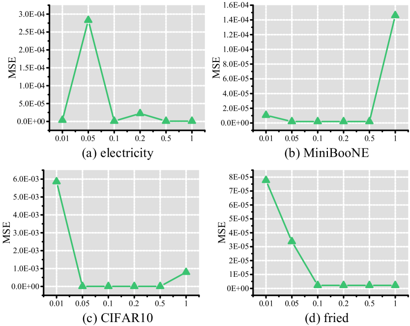
Figure 7: Results of sensitivity tests for the value of $\epsilon_{0}$ under incremental data valuation.

Table V displays the F1-scores of various data valuation approaches with two and three clusters on five classification datasets with 10% noise. Despite being adapted from AME, which performs poorly on mislabeled detection, GLOC achieves competitive performance on mislabeled data detection. Moreover, it consistently outperforms other Shapley value-based valuation approaches when the values are divided into three clusters. However, when data values are clustered into two clusters, GLOC performs less effectively compared to some other valuation methods. These findings indicate that these methods are likely to assign intermediate values to noisy samples. Fig. 6 illustrates the F1-scores of noise detection on another four datasets across various noise ratios. The results clearly demonstrate that our proposed GLOC approach consistently outperforms other methods across various noise ratios and datasets.

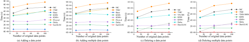
Figure 8: Comparison of time consumption between IncGLOC and DecGLOC and other compared baselines when adding or deleting one and multiple data points. DecGLOC and IncGLOC consistently exhibit the highest computational efficiency.

V-E Experiments on Incremental Data Valuation

This section examines the performance of IncGLOC when new samples are added to the original data. As with Section V-B, we adopt the average MSE to verify the effectiveness of the proposed algorithm. As there is only one study on dynamic data valuation [18], the methods included in our comparison are the same as those evaluated in that study. Specifically, the compared methods include MC, Base, TMC, Pivot-d, Delta, KNN, and KNN+. All the algorithms for compared methods can be seen in [18]. To determine the appropriate values for hyperparameters $\lambda$ and $\epsilon_{0}$, we partition $\mathcal{D}$ into the original and augmented components and then conduct incremental valuation by comparing MSEs across various settings of these hyperparameters. Subsequently, $\lambda$ and $\epsilon_{0}$ are determined to be 500 and 0.1, respectively. These settings have been validated as suitable across various datasets.

TABLE IX: MSEs of deleting a data point. The data values estimated by DecGLOC are the closest to the Shapley values, as indicated by the smallest MSEs.

Dataset	electricity	MiniBooNE	CIFAR10	fried
MC	5.56e-3	4.98e-5	4.89e-5	1.21e-5
TMC	4.43e-3	5.25e-4	5.77e-4	3.42e-4
YN-NN	3.45e-4	6.74e-5	8.93e-6	0.97e-5
Delta	3.89e-4	3.58e-5	2.78e-5	1.29e-5
KNN	7.65e-4	6.93e-6	6.79e-6	4.32e-5
KNN+	2.48e-4	5.67e-6	3.74e-5	4.56e-5
DecGLOC	0.95e-4	2.00e-6	2.55e-6	2.27e-6

TABLE X: MSEs of deleting two data points.

Dataset	electricity	MiniBooNE	CIFAR10	fried
MC	1.67e-3	2.78e-4	4.38e-4	3.22e-4
TMC	6.73e-3	3.21e-4	8.91e-5	2.67e-5
YNN-NNN	5.25e-4	6.77e-5	4.78e-6	2.13e-5
Delta	4.36e-4	5.43e-5	6.44e-6	4.55e-5
KNN	5.03e-4	7.85e-6	5.62e-5	8.97e-6
KNN+	2.56e-4	3.98e-6	3.45e-5	3.99e-5
DecGLOC	1.34e-4	2.86e-6	2.59e-6	2.01e-6

TABLE XI: Results of sensitivity tests for the value of $\lambda$ under decremental data valuation.

$\lambda$	electricity	MiniBooNE	CIFAR10	fried
1	0.52	0.62	11.26	0.85
10	3.00e-2	1.75e-4	4.23e-4	2.22e-4
50	5.62e-4	3.81e-5	7.31e-5	2.56e-5
100	2.80e-4	1.95e-5	1.68e-5	2.15e-5
500	1.22e-4	2.00e-6	2.55e-6	4.34e-6
1000	0.95e-4	3.76e-6	2.38e-6	2.27e-6

Tables VI and VII represent the comparison results of adding one and two points, respectively. From the results, our proposed IncGLOC consistently achieves the lowest MSEs across various datasets, indicating its effectiveness in Shapley value estimation under incremental valuation. Specifically, the data values estimated by IncGLOC are the most similar to the benchmark Shapley values. Moreover, MC and TMC perform the worst. While Delta, KNN, and KNN+ show improved performance compared to baselines such as MC and Base, they are unable to surpass our approach. This is attributed to our incorporation of global and local statistical information in data valuation. Additionally, to evaluate the computational efficiency of IncGLOC, we compare the computational time of different methods, as shown in Figs. 8(a) and (b). Due to the fact that methods such as Base, KNN, and KNN+, solely derive the updated data values from current values, their time consumption is low. However, Shapley value-based approaches like MC and TMC need substantial time for incremental data valuation, even only adding one data point. Nevertheless, our approach significantly enhances calculation efficiency, which typically requires just several minutes to compute the updated values for all data points.

Sensitivity tests for the hyperparameters in IncGLOC, including $\lambda$ and $\epsilon_{0}$, are also conducted. From Table VIII, IncGLOC achieves satisfactory performance when $\lambda$ is greater than or equal to 500. Additionally, as illustrated in Fig. 7, the performance of IncGLOC is stable when $\epsilon_{0}$ lies in the range of [0.1, 0.5]. Therefore, the hyperparameters can be set within these stable ranges.

V-F Experiments on Decremental Data Valuation

This section assesses the performance of DecGLOC in data valuation when some data points are removed from the original dataset. The experimental settings are consistent with those in the preceding subsection. Following previous research [18], the compared methods include MC and TMC, YN-NN (YNN-NNN for deleting multiple data points), Delta, a variant of KNN, and a variant of KNN+. The algorithms of all compared methods can be found in [18]. Tables IX and X present the comparison results of deleting one and two points, respectively. DecGLOC achieves the lowest MSEs, indicating the effectiveness of DecGLOC in decremental data valuation. Besides, MC and TMC perform the worst. Although KNN and KNN+ are the strongest baselines, their performance is inferior to ours. Additionally, we compare the calculation time of different methods, as shown in Figs. 8(c) and (d). Our proposed DecGLOC approach only consumes hundreds of seconds, which is the most efficient. However, the Shapley value-based approaches including MC, TMC, and Delta need substantial time for decremental data valuation, even only deleting one training point.

Sensitivity tests for the hyperparameters in DecGLOC, including $\lambda$ and $\epsilon_{0}$ are conducted. From Table XI, the performance of DecGLOC is favorable when $\lambda$ equals to and greater than 500. Furthermore, unlike IncGLOC, our sensitivity tests reveal that DecGLOC performs consistently stable when $\epsilon_{0}$ is selected from [0.01, 1]. Hence, its value can be randomly selected from this extensive range. Additionally, we compute the $p$-value [39, 40] of the differences between the MSEs of our algorithms and other approaches for all experiments. All $p$-values are smaller than 0.05, confirming the statistical significance of the difference.

VI Conclusion

This study proposes to integrate global and local statistical information of data values into data valuation, a perspective often overlooked by previous methods. By investigating the characteristics of value distributions, we introduce a new data valuation approach based on AME by incorporating these distribution characteristics. Additionally, we propose two dynamic data valuation algorithms for incremental and decremental data valuation, respectively, which compute data values solely based on the original and updated datasets, along with the original data values. Importantly, they do not require additional Shapley value estimation steps, thereby ensuring efficiency. Extensive experiments across various tasks, including Shapley value estimation, point addition and removal, mislabeled data detection, and incremental and decremental data valuation, validate the effectiveness and efficiency of our proposed methodologies.

References

- [1] R. Y. Wang, V. C. Storey, and C. P. Firth, “A framework for analysis of data quality research,” IEEE Trans. Knowl. Data Eng., vol. 7, no. 4, pp. 623–640, 1995.
- [2] I. N. Chengalur-Smith, D. P. Ballou, and H. L. Pazer, “The impact of data quality information on decision making: An exploratory analysis,” IEEE Trans. Knowl. Data Eng., vol. 11, no. 6, pp. 853–864, 1999.
- [3] A. Ghorbani, M. Kim, and J. Zou, “A distributional framework for data valuation,” in Proc. Int. Conf. Mach. Learn., 2020, pp. 3535–3544.
- [4] J. Pei, “A survey on data pricing: From economics to data science,” IEEE Trans. Knowl. Data Eng., vol. 34, no. 10, pp. 4586–4608, 2022.
- [5] K. F. Jiang, W. Liang, J. Zou, and Y. Kwon, “Opendataval: A unified benchmark for data valuation,” in Proc. Int. Conf. Neural Inf. Process. Syst., 2023.
- [6] Y. Kwon and J. Zou, “Beta shapley: A unified and noise-reduced data valuation framework for machine learning,” in Proc. Int. Conf. Artif. Intell. Stat., 2022, pp. 8780–8802.
- [7] J. Lin, A. Zhang, M. Lécuyer, J. Li, A. Panda, and S. Sen, “Measuring the effect of training data on deep learning predictions via randomized experiments,” in Proc. Int. Conf. Mach. Learn., 2022, pp. 13 468–13 504.
- [8] P. W. Koh and P. Liang, “Understanding black-box predictions via influence functions,” in Proc. Int. Conf. Mach. Learn., 2017, pp. 1885–1894.
- [9] H. A. Just, F. Kang, T. Wang, Y. Zeng, M. Ko, M. Jin, and R. Jia, “Lava: Data valuation without pre-specified learning algorithms,” in Proc. Int. Conf. Learn. Representations, 2023.
- [10] J. Yoon, S. Arik, and T. Pfister, “Data valuation using reinforcement learning,” in Proc. Int. Conf. Mach. Learn., 2020, pp. 10 842–10 851.
- [11] Y. Kwon and J. Zou, “Data-oob: Out-of-bag estimate as a simple and efficient data value,” in Proc. Int. Conf. Mach. Learn., 2023, pp. 18 135–18 152.
- [12] E. Winter, “The shapley value,” Handbook of Game Theory with Economic Applications, vol. 3, pp. 2025–2054, 2002.
- [13] A. E. Roth, “Introduction to the shapley value,” The Shapley Value, pp. 1–28, 1988.
- [14] M. Stoian, “Fast joint shapley values,” in Proc. Compan. Int. Conf. Manag. Data, 2023, pp. 285–287.
- [15] X. Luo, J. Pei, C. Xu, W. Zhang, and J. Xu, “Fast shapley value computation in data assemblage tasks as cooperative simple games,” Proc. ACM Manag. Data, vol. 2, no. 1, pp. 1–28, 2024.
- [16] A. Ghorbani and J. Zou, “Data shapley: Equitable valuation of data for machine learning,” in Proc. Int. Conf. Mach. Learn., 2019, pp. 2242–2251.
- [17] R. Jia, D. Dao, B. Wang, F. A. Hubis, N. M. Gurel, B. Li, C. Zhang, C. Spanos, and D. Song, “Efficient task-specific data valuation for nearest neighbor algorithms,” in Proc. VLDB Endow., 2019, pp. 1610–1623.
- [18] J. Zhang, H. Xia, Q. Sun, J. Liu, L. Xiong, J. Pei, and K. Ren, “Dynamic shapley value computation,” in Proc. Int. Conf. Data Eng., 2023, pp. 639–652.
- [19] M. Fleckenstein, A. Obaidi, and N. Tryfona, “A review of data valuation approaches and building and scoring a data valuation model,” Harvard Data Sci. Rev., vol. 5, no. 1, 2023.
- [20] R. H. L. Sim, X. Xu, and B. K. H. Low, “Data valuation in machine learning:”ingredients”, strategies, and open challenges,” in Proc. Int. Joint Conf. Artif. Intell., 2022, pp. 5607–5614.
- [21] W. Liang and J. Zou, “Metashift: A dataset of datasets for evaluating contextual distribution shifts and training conflicts,” in Proc. Int. Conf. Learn. Representations, 2022.
- [22] C. G. Northcutt, A. Athalye, and J. Mueller, “Pervasive label errors in test sets destabilize machine learning benchmarks,” in Proc. Int. Conf. Neural Inf. Process. Syst., 2021.
- [23] J. T. Wang and R. Jia, “Data banzhaf: A robust data valuation framework for machine learning,” in Proc. Int. Conf. Artif. Intell. Stat., 2023, pp. 6388–6421.
- [24] V. Feldman and C. Zhang, “What neural networks memorize and why: Discovering the long tail via influence estimation,” in Proc. Int. Conf. Neural Inf. Process. Syst., 2020, pp. 2881–2891.
- [25] V. Shah and S. Shukla, “Data distribution into distributed systems, integration, and advancing machine learning,” Rev. Esp. Doc. Cient., vol. 11, no. 1, pp. 83–99, 2017.
- [26] Y. Guo, W. Wang, and X. Wang, “A robust linear regression feature selection method for data sets with unknown noise,” IEEE Trans. Knowl. Data Eng., vol. 35, no. 1, pp. 31–44, 2023.
- [27] T. Evgeniou and M. Pontil, “Regularized multi-task learning,” in Proc. Int. Conf. Knowl. Discov. Data Mining, 2004, pp. 109–117.
- [28] L. E. Peterson, “K-nearest neighbor,” Scholarpedia, vol. 4, no. 2, p. 1883, 2009.
- [29] F. Zhu, J. Gao, J. Yang, and N. Ye, “Neighborhood linear discriminant analysis,” Pattern Recognit., vol. 123, p. 108422, 2022.
- [30] Z. Zhong, E. Fini, S. Roy, Z. Luo, E. Ricci, and N. Sebe, “Neighborhood contrastive learning for novel class discovery,” in Proc. IEEE Conf. Comput. Vis. Pattern Recognit., 2021, pp. 10 867–10 875.
- [31] J. Gama, P. Medas, G. Castillo, and P. Rodrigues, “Learning with drift detection,” in Proc. Brazilian Symp. Artif. Intell., 2004, pp. 286–295.
- [32] A. Krizhevsky, G. Hinton et al., “Learning multiple layers of features from tiny images,” Handbook of Systemic Autoimmune, 2009.
- [33] A. Justel, D. Peña, and R. Zamar, “A multivariate kolmogorov-smirnov test of goodness of fit,” Stat. Probab. Lett., vol. 35, no. 3, pp. 251–259, 1997.
- [34] D. Greene and P. Cunningham, “Practical solutions to the problem of diagonal dominance in kernel document clustering,” in Proc. Int. Conf. Mach. Learn., 2006, pp. 377–384.
- [35] X. Xu, Z. Wu, C. S. Foo, and B. K. H. Low, “Validation free and replication robust volume-based data valuation,” in Proc. Int. Conf. Neural Inf. Process. Syst., 2021, pp. 10 837–10 848.
- [36] V. Sanh, L. Debut, J. Chaumond, and T. Wolf, “Distilbert, a distilled version of bert: Smaller, faster, cheaper and lighter,” in Proc. Int. Conf. Neural Inf. Process. Syst., 2019.
- [37] K. He, X. Zhang, S. Ren, and J. Sun, “Deep residual learning for image recognition,” in Proc. IEEE Conf. Comput. Vis. Pattern Recognit., 2016, pp. 770–778.
- [38] H. Xiong, G. Pandey, M. Steinbach, and V. Kumar, “Enhancing data analysis with noise removal,” IEEE Trans. Knowl. Data Eng., vol. 18, no. 3, pp. 304–319, 2006.
- [39] S. Agarwal, S. Dutta, and A. Bhattacharya, “Chisel: Graph similarity search using chi-squared statistics in large probabilistic graphs,” in Proc. VLDB Endow., 2020, pp. 1654–1668.
- [40] W. J. Conover, Practical nonparametric statistics. John Wiley & Sons, 1999.