Ferrari: Federated Feature Unlearning via
Optimizing Feature Sensitivity

Abstract

The advent of Federated Learning (FL) highlights the practical necessity for the ’right to be forgotten’ for all clients, allowing them to request data deletion from the machine learning model’s service provider. This necessity has spurred a growing demand for Federated Unlearning (FU). Feature unlearning has gained considerable attention due to its applications in unlearning sensitive features, backdoor features, and bias features. Existing methods employ the influence function to achieve feature unlearning, which is impractical for FL as it necessitates the participation of other clients in the unlearning process. Furthermore, current research lacks an evaluation of the effectiveness of feature unlearning. To address these limitations, we define feature sensitivity in the evaluation of feature unlearning according to Lipschitz continuity. This metric characterizes the rate of change or sensitivity of the model output to perturbations in the input feature. We then propose an effective federated feature unlearning framework called Ferrari, which minimizes feature sensitivity. Extensive experimental results and theoretical analysis demonstrate the effectiveness of Ferrari across various feature unlearning scenarios, including sensitive, backdoor, and biased features.

1 Introduction

Federated Learning (FL) [1, 2, 3] allows for model training across decentralized devices or servers holding local private data samples, without the need to directly exchange them. An essential requirement within FL is the participants’ "right to be forgotten," as explicitly outlined in regulations such as the European Union General Data Protection Regulation (GDPR) and the California Consumer Privacy Act (CCPA) [4]. To address this requirement, Federated Unlearning (FU) has been introduced, enabling clients to selectively remove the influence of specific subsets of their data from a trained FL model. This process ensures the accuracy of the FL model is maintained on the remaining data [5].

Different from unlearning at the client, class, or sample level [6, 7, 8] in FL, the feature unlearning [9] holds significant applications across various scenarios. Firstly, in contexts where sentences contain sensitive information such as names and addresses [10, 11], it becomes crucial to remove these sensitive components in order to prevent potential exposure through model inversion attacks [12, 13, 14, 15]. Secondly, when datasets contain backdoor triggers that can compromise model integrity [16, 17, 18, 19], it is imperative to eliminate these patterns. Thirdly, in scenarios where data imbalances significantly impact model accuracy due to bias [20, 21, 22, 23], unlearning biased features becomes essential.

There are two challenges in feature unlearning in FL. Firstly, evaluating the unlearning effectiveness for feature unlearning is difficult. Typically, unlearning effectiveness is assessed by comparing the unlearned model with a retrained model without the feature. However, building data without the feature is challenging; for example, training the data with noise or a black block on the feature region may cause serious degradation in model accuracy (see Sec. 3.2). Secondly, previous work on feature unlearning within centralized machine learning settings [9, 10, 11] is not practical for federated learning due to its requirement for access to all datasets, necessitating the participation of all clients.

To address the aforementioned limitations, we first define the feature sensitivity in Sec. 4.1 to evaluate the feature unlearning inspired by the Lipschitz continuity, which characterizes the rate of change or sensitivity of the model output to perturbations in the input feature. Then we propose a simple but effective federated feature unlearning methods, called Ferrari (Federated Feature Unlearning), by minimizing the feature sensitivity in Sec. 4.2. Our Ferrari framework offers three key advantages: Firstly, Ferrari  requires only local datasets from the unlearned clients for feature unlearning. Secondly, Ferrari demonstrates high practicality and efficiency, which support various feature unlearning scenarios, including sensitive, backdoor, and biased features and only consumes a few epochs optimization. Thirdly, theoretical analysis in Sec. 4.3 elucidates that the proposed Ferrari  achieves the less model utility loss compared to the exact feature unlearning. The key contributions of this work are summarized as follows:

• We point out two challenges for feature unlearning in FL. One is how to unlearn feature successfully in FL without the participation of other clients in Sec. 3.2. The other is how to design an evaluation in federated feature unlearning.

• We define the feature sensitivity and introduce this metric in federated feature unlearning in Sec. 4. By minimizing feature sensitivity, we propose an effective federated feature unlearning method, called Ferrari, allowing clients to selectively unlearn specific features from the trained global model without the participation of other clients.

• We provide theoretical proof in Theorem 1, which dictates that Ferrari achieves better model performances than exact feature unlearning. This analytical result is also echoed in empirical result, in terms of Ferrari’s effectiveness in a variety of settings including sensitive, backdoor, and biased features unlearning.

2 Related Work

Machine Unlearning

Machine Unlearning (MU), introduced by Cao et al. [24], involves selectively removing specific training data from a trained model without retraining from scratch[25, 26]. It categorizes into exact unlearning [27, 28], aiming to completely remove data influence with techniques like SISA [29] and ARCANE [30], though with computational costs, and approximate unlearning [31, 32], which reduces data impact through techniques like data manipulation (fine-tuning with mislabeled data [33, 34, 35, 36, 37] or introducing noise [38, 39, 40]), knowledge distillation [41, 42, 43, 44] (training a student model), gradient ascent [45, 46, 47, 48] (maximizing loss associated with forgotten data), and weight scrubbing [49, 50, 51, 52, 53, 54] (discarding heavily influenced weights).

Federated Unlearning

In FL, traditional centralized MU methods are not suitable due to inherent differences like incremental learning and limited dataset access [55]. Research on Federated Unlearning (FU) mainly focuses on client, class, and sample unlearning [6, 7, 8]. Client unlearning, pioneered by Liu et al. [56] introducing FedEraser [56], includes approaches like FRU [57], FedRecover [58], VeriFI [59], HDUS [60], KNOT [61], FedRecovery [62], Knowledge Distillation [55], and Gradient Ascent [63, 64, 65], aiming to remove specific clients or recover poisoned global models. Class unlearning, introduced by Wang et al. [66], involves frameworks like discriminative pruning and Momentum Degradation [67] (MoDE) to remove entire data classes. Sample unlearning, initiated by Liu et al. [68], targets individual sample removal within FL settings, with advancements like the QuickDrop [69] framework and FedFilter [70] enhancing efficiency and effectiveness. Recent works, such as $FedMe^{2}$ by Xia et al. [71], optimize both unlearning facilitation and privacy guarantees.

Existing literature on FU primarily focuses on client, class, or sample unlearning [6, 7, 8]. However, a significant gap arises when a client seeks to remove only sensitive features while remaining engaged in FL. Unfortunately, current FU approaches do not address this specific scenario, as they do not explore feature unlearning within FL settings. In contrast to prior works focusing on feature unlearning in centralized settings of MU, such as classification models [9, 10, 11], generative models [72, 73, 74, 75], and large language models [76, 77, 78], this study uniquely addresses feature unlearning of classification model within the FL paradigm. This distinction arises because traditional feature unlearning methods in centralized settings of MU are impractical for FL scenarios, where participation from all clients is often infeasible. In such cases, if even a single client opts out of the operation, the process fails.

Therefore, to fill this critical gap, we proposed a novel federated feature unlearning framework namely Ferrari based on the concept of Lipschitz continuity [79, 80, 81]. Our proposed Ferrari exclusively requires participation from the target client’s dataset while preserving the model’s original performance. Lipschitz continuity, a foundational mathematical concept, measures the sensitivity of a function to changes in its input variables [82, 83, 84]. This concept plays a pivotal role in our feature unlearning methodology. For a detailed exposition of our proposed federated feature unlearning framework employing Lipschitz continuity (see Sec. 4). To the best of our knowledge, this represents the first work in feature unlearning within FL settings that does not necessitate participation from all clients, showcasing the potential to enhance privacy, practicality and efficiency.

3 Challenges on Feature Unlearning in FL

3.1 Federated Feature Unlearning

Consider a federated system comprising $K$ clients and one server, collaboratively learning a global model $f_{\theta}$ as:

$$\min_{\theta}\sum_{k=1}^{K}\sum_{i=1}^{n_{k}}\frac{\ell(f_{\theta}(x_{k,i}),y_{k,i})}{n_{1}+\cdots+n_{K}},$$ (1)

where $\ell$ is the loss, e.g., the cross-entropy loss, $\mathcal{D}_{k}=\{(x_{k,i},y_{k,i})\}_{i=1}^{n_{k}}$ is the dataset with size $n_{k}$ owned by client $k$. One client (i.e.,, referred to as the unlearn client $C_{u}$) requests the removal of a feature $\mathcal{F}$ from the global model $\theta$ such that the global model $\theta$ so that $\theta$ does not retain any information about $\mathcal{F}$. Specifically, we assume that the data $x\in\mathbb{R}^{d}$ and denote the j-th feature of $x$ by $x[j]$. The partial element of the data $x$ corresponding the feature $\mathcal{F}$ is defined as $x[\mathcal{F}]$, i.e.,:

$$x[\mathcal{F}]=\{x[j],j\in\mathcal{F}\}$$ (2)

Therefore, the unlearn client $C_{u}$ aims to remove $\{x_{i,u}[\mathcal{F}]\}_{i=1}^{n_{u}}$, called unlearned data $\mathcal{D}_{u}$. Denote $\mathcal{D}_{r}=\mathcal{D}-\mathcal{D}_{u}$ to be the remaining data.

3.2 Challenges for Feature Unlearning in FL

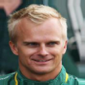
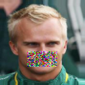
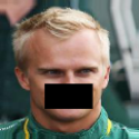
$x$ $\overline{x}_{G}$ $\overline{x}_{B}$ Acc 95.86% 75.51% 68.37%

Figure 1: Sample data $x$, perturbed with Gaussian noise ($\overline{x}_{G}$) and with black pixels ($\overline{x}_{B}$) in the target region, illustrate feature removal with the corresponding performance comparison.

Unlike sample or class unlearning [6, 7, 8], evaluating the unlearning effectiveness for feature unlearning is difficult. Typically, unlearning effectiveness is assessed by comparing the unlearned model with a retrained model that is trained on remaining data $\mathcal{D}_{r}$. However, it is hard to build $\mathcal{D}_{r}$ for the feature unlearning. For example, if we want to remove the mouth from a face image, one possible solution is to replace the mouth region with Gaussian noise or black block, as illustrated in Fig. 1. However, this added Gaussian noise or black block can adversely affect model training and degrade performance, e.g., the degradation of model accuracy is beyond 27% as demonstrated in Fig. 1.

Another challenge is implementing feature unlearning for $C_{u}$ without the help of other clients. Previous work on feature unlearning [9, 10, 11] typically requires access to the remaining data, necessitating the participation of other clients in the FL process. This requirement is impractical in the FL context, where each client may not be willing or able to share data or computational resources. Therefore, finding a method to effectively unlearn features without relying on other clients is crucial to maintaining model accuracy and practicality in FL settings.

4 The Proposed Method

In this section, we introduce feature sensitivity (see Def. 1) in Sec. 4.1 to evaluate feature unlearning effectiveness. We then propose Ferrari based on this concept in Sec. 4.2). Finally, we demonstrate that Ferrari achieves less utility loss compared to exact feature unlearning in Sec. 4.3).

4.1 Feature Sensitivity

Algorithm 1 Federated Feature Unlearning

1:Input: Unlearned client $u$, Local dataset $\mathcal{D}_{u}$ with data size $n_{u}$, Unlearn feature $\{\mathcal{F}_{i}\}_{i=1}^{N}$, Global model parameters $\theta$, Gaussian noise $\sigma$, Learning rate $\eta$, Sample number $N$

2:Output: Unlearned model parameters $\theta^{u}$

3:$\triangleright$ The unlearned client $k$ performs:

4:for $(x,\mathcal{F}_{i})$ in $(\mathcal{D}_{u},\{\mathcal{F}_{i}\}_{i=1}^{N})$ do

5:     $\theta^{u}=\theta$

6:     for $i=1$ to $N$ do

7:         Sample $\delta_{\mathcal{F}_{i}}$ according to Eq. (4)

8:         Compute $L_{i}=\frac{\|f_{\theta^{u}}(x)-f_{\theta^{u}}(x+\delta_{\mathcal{F},i})\|_{2}}{\|\delta_{\mathcal{F},i}\|_{2}}$

9:     end for

10:     $L=\frac{1}{N}\sum_{i=1}^{N}L_{i}$

11:     $\theta^{u}\leftarrow\theta^{u}-\eta\cdot\nabla_{\theta^{u}}(L)$

12:end for

13:Upload $\theta^{u}$ to the server

14:$\triangleright$ The server performs:

15:Replace the global model $\theta$ with the $\theta^{u}$

16:return $\theta^{u}$

Inspired by Lipschitz continuity [80, 81, 83], which provides an approximate method for removing information from images by perturbing the input data and observing the effect on the output, we introduce the concept of feature sensitivity $s$ as Def. 1. This metric measures the memorization of a model $f_{\theta}$ for the feature $\mathcal{F}$ by considering the local changes in the given input rather than the global change as defined in the traditional Lipschitz continuity.

Definition 1.

The feature sensitivity $s$ of the model $f$ with respect to the feature $\mathcal{F}$ on the data $(x,y)$ is defined as:

$$s=\mathbb{E}_{\delta_{\mathcal{F}}}\frac{\|f(x)-f(x+\delta_{\mathcal{F}})\|_{2}}{\|\delta_{\mathcal{F}}\|_{2}},$$ (3)

where $\delta_{\mathcal{F}}$ denote the perturbation on feature $\mathcal{F}$.

Def. 1 characterizes the rate of change or sensitivity of the model output to perturbations in the input data. A small feature sensitivity $s$ represents the model $f$ doesn’t memorize the feature $\mathcal{F}$. This definition does not require building the remaining data, as it considers the expectation over the perturbation $\delta_{\mathcal{F}}$. Specifically, it represents the average rate of change of the output over any magnitude of the perturbation. Furthermore, we will provide the relationship between Def. 1 and exact feature unlearning in Sec. 4.3.

Remark 1.

The perturbation $\delta_{\mathcal{F}}$ can be chosen from various distributions, such as the Gaussian distribution, the uniform distribution, and so on.

4.2 Ferrari

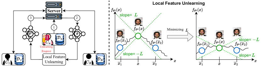
Figure 2: Overview of our proposed Ferrari framework: Initiated by the feature unlearning request from the unlearn client $C_{u}$, the server initializes the trained global model $\theta$ to $C_{u}$ for local feature unlearning. Upon completion, $C_{u}$ uploads the unlearned model $\theta^{u}$ to the server. Local feature unlearning minimizes the Lipschitz constant $L$ between the original input and its perturbed feature subset, reducing feature sensitivity while maintaining overall model performance.

As discussed about the feature sensitivity $s$ in Sec. 4.1, the core idea of the proposed method Ferrari is to achieve the feature unlearning by minimizing the feature sensitivity. More specifically, it controls the change of model output in terms of input change in feature region i.e., the slope to let the model not memorize the feature as illustrated in Fig. 2.

One unlearning client $C_{u}$ requests to unlearning the feature $\mathcal{F}$. The proposed Ferrariaims to unlearn the global model $\theta$ to $\theta^{u}$. The proposed method can be divided into three steps (see details in Alg. 1). In order to compute the feature sensitivity, the perturbation $\delta_{\mathcal{F}}$ in terms of the feature $\mathcal{F}$ is firstly computed as the following (take the Gaussian distribution as an example):

$$\delta_{\mathcal{F}}[j]=\left\{\begin{aligned} \sim N(0,\sigma^{2})\quad&j\in\mathcal{F}\\ 0\qquad\qquad&\text{Otherwise}\\ \end{aligned}\right.$$ (4)

Secondly, we leverage a finite sample Monte Carlo approximation to the maximization as Def. 1 as:

$$\begin{split}\mathbb{E}_{\delta_{\mathcal{F}}}\frac{\|f_{\theta}(x)-f_{\theta}(x+\delta_{\mathcal{F}})\|_{2}}{\|\delta_{\mathcal{F}}\|_{2}}\sim\frac{1}{N}\sum_{i=1}^{N}\frac{\|f_{\theta}(x)-f_{\theta}(x+\delta_{\mathcal{F},i})\|_{2}}{\|\delta_{\mathcal{F},i}\|_{2}},\end{split}$$ (5)

where $\delta_{\mathcal{F},i}$ is $i_{th}$ sampling as Eq. (4).

Finally, for the unlearning client $C_{u}$ who aims to remove the feature $\mathcal{F}$ from his data $\mathcal{D}_{u}$, the unlearned model $\theta^{u}$ is obtained as the following:

$$\theta^{u}=\operatorname*{arg\,min}_{\theta}\mathbb{E}_{(x,y)\in\mathcal{D}_{u}}\frac{1}{N}\sum_{i=1}^{N}\frac{\|f_{\theta}(x)-f_{\theta}(x+\delta_{\mathcal{F},i})\|_{2}}{\|\delta_{\mathcal{F},i}\|_{2}},$$ (6)

where Eq. (6) is computed over the dataset $\mathcal{D}_{u}$. Noted that the proposed Ferrari based on Def. 1 doesn’t need the participation of other clients.

Remark 2.

When the unlearning happens during the federated training, the unlearning clients would also optimize the training loss and feature sensitivity simultaneously, i.e., $\mathbb{E}_{(x,y)\in\mathcal{D}}\big{(}\ell(f_{\theta}(x),y)+\lambda\mathbb{E}_{\delta_{\mathcal{F}}}\frac{\|f_{\theta}(x)-f_{\theta}(x+\delta_{\mathcal{F}})\|_{2}}{\|\delta_{\mathcal{F}}\|_{2}}\big{)},$ where $\lambda$ is a coefficient.

4.3 Theoretical Analysis of the Utility loss for Ferrari

As illustrated in Sec. 3.2, retraining the model without the feature may influence the model accuracy seriously. Suppose the feature is successfully removed when the norm of perturbation is larger than $C$. We firstly define the utility loss $\ell_{1}$ with unlearning feature directly, i.e., the exact feature unlearning:

$$\ell_{1}=\min_{\|\delta_{\mathcal{F}}\|\geq C}\mathbb{E}_{(x,y)\in\mathcal{D}}\min_{\theta}\ell\big{(}f_{\theta}(x+\delta_{\mathcal{F}}),y\big{)}$$ (7)

And we define the maximum utility loss with the norm perturbation less than $C$ as:

$$\ell_{2}=\max_{\|\delta_{\mathcal{F}}\|\leq C}\mathbb{E}_{(x,y)\in\mathcal{D}}\min_{\theta}\ell\big{(}f_{\theta}(x+\delta_{\mathcal{F}}),y\big{)}$$ (8)

Assumption 1.

Assume $\ell_{2}\leq\ell_{1}$

Assumption 1 elucidates that the utility loss associated with a perturbation norm less than $C$ is smaller than the utility loss when the perturbation norm is greater than $C$. This assumption is logical, as larger perturbations would naturally lead to greater utility loss.

Assumption 2.

Suppose the federated model achieves zero training loss.

We have the following theorem to elucidate the relation between feature sensitivity removing via Algo. 1 and exact unlearning (see proof in Appendix A.1).

Theorem 1.

If Assumption 1 and 2 hold, the utility loss of unlearned model obtained by Algo. 1 is less than the utility loss with unlearning successfully, i.e.,

$$\ell_{u}\leq\ell_{1},$$ (9)

where $\ell_{u}=\mathbb{E}_{(x,y)\in\mathcal{D}}\ell(f_{\theta^{u}}(x),y)$

Theorem 1 showcases that the proposed method Ferrari, results in a utility loss ( $\ell_{u}$) that is less than the utility loss incurred when the feature is removed and the model is retrained, i.e., the process of exact feature unlearning.

Remark 3.

To further evaluate the effectiveness of feature unlearning based on feature sensitivity, we employ model inversion attacks [12, 13] to determine if the feature can be reconstructed and utilize attention maps to assess whether the model still focuses on the unlearned feature, as described in Sec. 5.3.1.

5 Experimental Results

This section presents the empirical analysis of the proposed Ferrari framework in terms of effectiveness, utility, and time efficiency in sensitive, backdoor and biased feature unlearning scenarios.

5.1 Experimental Setup

MNIST FMNIST CIFAR-10 CIFAR-20 CIFAR-100

Figure 3: Pixel-pattern backdoor feature.

CMNIST CelebA

Figure 4: Biased datasets distribution.

Unlearning Scenarios

Sensitive Feature Unlearning: We simulate the removal of sensitive features from the $\mathcal{D}_{u}$ to fulfill the request of $C_{u}$ due to privacy concern. Specifically, we remove ’mouth’ from CelebA [85], ’marital status’ from Adult [86], and ’pregnancies number’ from Diabetes [87]. Therefore, our proposed Ferrari aims to remove the influence of these requested features.

Backdoor Feature Unlearning: We simulate a pixel-pattern backdoor attack by $C_{u}$ based on BadNets [19] within a FL framework [16, 17, 18]. $C_{u}$ injects a pixel-pattern backdoor feature and trigger label into its $\mathcal{D}_{u}$ during training, as shown in Fig. 4. Consequently, our proposed Ferrari aims to remove the influence of these backdoor features and restore the model’s original performance.

Biased Feature Unlearning: We simulate the bias dataset $\mathcal{D}_{u}$ of the $C_{u}$ and the unbias dataset $\mathcal{D}_{r}$ with a bias ratio of 0.8, as shown in Fig. 4. This results in a global model biased towards the biased dataset [88, 89] due to unintended feature memorization [23]. In CMNIST [90], the model focuses on color patterns instead of digits, and in CelebA [85], it learns mouth features instead of facial features for gender classification. Therefore, our proposed Ferrari aims to mitigate this bias-inducing features and restore model performance.

Hyperparameters & Datasets & Model

We simulate HFL with $K=10$ clients under an IID setting, each holding $10\%$ of the datasets, except for the biased feature unlearning experiment with a bias ratio of 0.8. For federated feature unlearning experiments, we set hyperparameters: learning rate $\eta=0.0001$, sample size $N=20$, and random Gaussian noise with standard deviation ranging from $0.05\leq\sigma\leq 1.0$ (see Sec. 5.5) across iterations of $N$. Experiments are repeated over five random trials, and results are reported as mean and standard deviation. We employ ResNet18 [91] on image datasets: MNIST [90], Colored-MNIST (CMNIST) [90], Fashion-MNIST [92], CIFAR-10, CIFAR-20, and CIFAR-100 [93], and a fully-connected neural network linear model on tabular datasets: Adult Census Income (Adult) [86] and Diabetes [87]. Further details are in Appendix A.2.

Evaluation Metrics

We assess effectiveness by measuring feature sensitivity (see Section 4.1) and conducting a model inversion attack (MIA)[12, 13, 14, 15] to determine the attack success rate (ASR). The goal is to achieve low feature sensitivity and low ASR, indicating successful unlearning of sensitive features. Backdoor and biased feature unlearning are evaluated by comparing accuracy on the retain dataset $\mathcal{D}_{r}$ ($Acc_{r}$) and the unlearn client dataset $\mathcal{D}_{u}$($Acc_{u}$). Low $Acc_{u}$ indicates high effectiveness for backdoor unlearning, while similar accuracy ($Acc_{r}\approx Acc_{u}$) reflects fairness and effectiveness in biased feature unlearning. Qualitatively, effectiveness is assessed using MIA-reconstructed images (sensitive) and GradCAM[94] attention maps (backdoor and biased). Utility is measured by test dataset $\mathcal{D}_{t}$ accuracy ($Acc_{t}$), with higher values indicating stronger utility. Time efficiency is evaluated by comparing the runtime of each baseline

Baselines

We compare our proposed Ferrari against the models of Baseline, Retrain, Fine-tune, FedCDP[66] and FedRecovery[62]. Additional details are provided in Appendix A.2.

5.2 Utility Guarantee

To evaluate the utility of Ferrari, we measure $Acc_{t}$ on $\mathcal{D}_{t}$, where a higher $Acc_{t}$ indicates greater utility (Tab. 1). Although the Fine-tune method shows high $Acc_{t}$ in the backdoor feature unlearning scenario with a clean dataset, its unlearning effectiveness is very low (see Sec. 5.3.2). This problem worsens with FedCDP[66] and FedRecovery[62], which suffer significant $Acc_{t}$ declines, reducing model utility and making them unsuitable for feature unlearning. In contrast, Ferrari achieves the highest model utility in sensitive and biased feature unlearning scenarios, with the highest $Acc_{t}$ among baselines, minimal deterioration, and the greatest unlearning effectiveness across all scenarios.

Scenarios Datasets Unlearn Feature Accuracy(%) Baseline Retrain Fine-tune FedCDP[66] RedRecovery[62] Ferrari (Ours) Sensitive CelebA Mouth 94.87 $\pm$1.38 79.46 $\pm$2.32 62.79 $\pm$1.62 34.03 $\pm$4.20 29.78 $\pm$6.69 92.26 $\pm$1.73 Adult Marriage 82.45 $\pm$2.59 65.27 $\pm$0.58 61.02 $\pm$1.05 30.19 $\pm$1.62 27.89 $\pm$3.71 81.02 $\pm$0.58 Diabetes Pregnancies 82.11 $\pm$0.49 64.19 $\pm$0.72 59.57 $\pm$0.68 36.71 $\pm$4.56 17.56 $\pm$2.32 79.53 $\pm$0.79 Backdoor MNIST Backdoor Pixel Pattern 94.75 $\pm$4.88 96.23 $\pm$0.16 96.85 $\pm$0.91 65.31 $\pm$4.39 40.52 $\pm$7.38 95.83 $\pm$1.14 FMNIST 90.68 $\pm$2.19 92.98 $\pm$0.75 93.52 $\pm$1.63 67.62 $\pm$0.81 42.24 $\pm$4.45 92.61 $\pm$1.57 CIFAR-10 87.55 $\pm$3.71 90.92 $\pm$1.83 91.23 $\pm$0.44 53.98 $\pm$2.17 27.16 $\pm$9.68 89.52 $\pm$2.18 CIFAR-20 74.47 $\pm$2.38 81.61 $\pm$1.75 82.52 $\pm$0.69 54.76 $\pm$0.98 23.02 $\pm$3.11 78.34 $\pm$2.35 CIFAR-100 54.13 $\pm$7.62 73.12 $\pm$1.54 73.59 $\pm$1.66 34.30 $\pm$0.42 15.21 $\pm$5.83 69.30 $\pm$2.27 Bias CMNIST Color 81.72 $\pm$3.41 98.49 $\pm$1.46 82.54 $\pm$0.78 27.56 $\pm$1.71 25.05 $\pm$5.09 83.85 $\pm$1.63 CelebA Mouth 87.35 $\pm$4.07 95.87 $\pm$1.52 88.93 $\pm$2.65 16.98 $\pm$0.23 20.19 $\pm$7.21 94.62 $\pm$2.49

Table 1: The accuracy of $\mathcal{D}_{t}$ for each unlearning method across different unlearning scenarios.

5.3 Effectiveness Guarantee

In this subsection, we analyze the unlearning effectiveness of Ferrari against baselines in sensitive, backdoor, and biased feature unlearning scenarios.

5.3.1 Sensitive Feature Unlearning

To evaluate Ferrari’s effectiveness in unlearning sensitive features, we measured feature sensitivity (see Sec. 4.1) and conducted a model inversion attack (MIA) [12, 13, 14, 15].

Scenario Datasets Unlearn Feature Feature Sensitivity Baseline Retrain Fine-tune FedCDP [66] FedRecovery [62] Ferrari  (Ours) Sensitive CelebA Mouth 0.96 $\pm$1.41$\times 10^{-2}$ 0.07 $\pm$8.06$\times 10^{-4}$ 0.79 $\pm$2.05$\times 10^{-2}$ 0.93 $\pm$2.87$\times 10^{-2}$ 0.91$\pm$3.41$\times 10^{-2}$ 0.09 $\pm$3.04$\times 10^{-4}$ Adult Marriage 1.31 $\pm$1.53$\times 10^{-2}$ 0.02 $\pm$6.47$\times 10^{-4}$ 0.94 $\pm$6.81$\times 10^{-2}$ 1.07 $\pm$7.43$\times 10^{-2}$ 1.14 $\pm$2.57$\times 10^{-2}$ 0.05 $\pm$1.72$\times 10^{-4}$ Diabetes Pregnancies 1.52 $\pm$0.91$\times 10^{-2}$ 0.05 $\pm$5.07$\times 10^{-4}$ 0.96 $\pm$1.28$\times 10^{-2}$ 1.23 $\pm$3.82$\times 10^{-2}$ 0.83 $\pm$5.08$\times 10^{-2}$ 0.07 $\pm$1.07$\times 10^{-4}$

Table 2: Feature sensitivity for each unlearning method across sensitive feature unlearning scenario.

Feature Sensitivity

Tab. 2 shows the sensitivity of the unlearn feature. The baseline model had high sensitivity to this feature. Similar results were observed for the Fine-tune, FedCDP [66], and FedRecovery models [62], with sensitivities greater than 0.8, indicating ineffective unlearning. In contrast, our proposed Ferrari model exhibits low sensitivity, similar to the Retrain model, indicating successful unlearning of the sensitive feature.

Scenario Datasets Unlearn Feature Attack Success Rate(ASR) ($\%$) Baseline Retrain Fine-tune FedCDP [66] FedRecovery [62] Ferrari(Ours) Sensitive CelebA Mouth 84.36 $\pm$3.22 47.52 $\pm$1.04 77.43 $\pm$10.98 75.36 $\pm$9.31 71.52 $\pm$6.07 51.28 $\pm$2.41 Adult Marriage 87.54 $\pm$13.89 49.28 $\pm$2.13 83.45 $\pm$8.44 72.83 $\pm$5.18 80.39 $\pm$10.68 49.58 $\pm$1.38 Diabetes Pregnancies 92.31 $\pm$7.55 38.89 $\pm$2.52 88.46 $\pm$5.01 81.91 $\pm$8.17 78.27 $\pm$2.47 42.61 $\pm$1.81

Table 3: The ASR of MIA for each unlearning method across sensitive feature unlearning scenario.

ASR of MIA

Tab. 3 shows the ASR results. The Baseline model achieved an ASR exceeding 80%, indicating substantial exposure of sensitive features. Similar observations were made for the Fine-tune, FedCDP [66], and FedRecovery [62] models, with ASR surpassing 70% exhibiting ineffective feature unlearning. Conversely, Ferrari achieved low ASR, suggesting successful feature unlearning with minimal unlearned feature exposure after using Ferrari via MIA.

Target Baseline Retrain Ferrari Target Baseline Retrain Ferrari

Table 4: MIA reconstruction on CelebA (unlearned mouth)

MIA Reconstruction

Fig. 4 shows MIA-reconstructed images. The Baseline model achieved complete reconstruction, whereas both Retrain and Ferrari models failed to accurately reconstruct the mouth feature. This underscores Ferrari’s effectiveness in unlearning and preserving privacy by preventing precise reconstruction of unlearned features via MIA.

5.3.2 Backdoor Feature Unlearning

Scenarios Datasets Unlearn Feature Accuracy (%) Baseline Retrain Fine-tune FedCDP[66] RedRecovery[62] Ferrari(Ours) Backdoor MNIST Backdoor pixel-pattern $\mathcal{D}_{r}$ 95.65 $\pm$1.39 97.19 $\pm$2.49 96.16 $\pm$0.37 65.82 $\pm$6.85 40.81 $\pm$4.31 95.93 $\pm$0.45 $\mathcal{D}_{u}$ 97.43 $\pm$3.69 0.00 $\pm$0.00 72.64 $\pm$0.24 69.37 $\pm$0.83 53.72 $\pm$3.14 0.11 $\pm$0.01 FMNIST $\mathcal{D}_{r}$ 91.07 $\pm$0.54 93.85 $\pm$1.08 94.36 $\pm$1.98 68.46 $\pm$3.39 42.93 $\pm$2.50 92.83 $\pm$0.61 $\mathcal{D}_{u}$ 94.51 $\pm$6.29 0.00 $\pm$0.00 43.91 $\pm$0.28 72.19 $\pm$0.49 48.15 $\pm$4.37 0.90 $\pm$0.03 CIFAR-10 $\mathcal{D}_{r}$ 87.63 $\pm$1.16 91.12 $\pm$1.60 92.02 $\pm$3.15 54.91 $\pm$6.91 27.49 $\pm$4.96 89.91 $\pm$0.95 $\mathcal{D}_{u}$ 95.05 $\pm$2.30 0.00 $\pm$0.00 88.44 $\pm$0.92 62.75 $\pm$5.07 49.26 $\pm$2.23 0.29 $\pm$0.04 CIFAR-20 $\mathcal{D}_{r}$ 75.06 $\pm$6.41 81.91 $\pm$4.68 82.67 $\pm$1.32 55.67 $\pm$6.35 23.76 $\pm$2.17 78.29 $\pm$3.12 $\mathcal{D}_{u}$ 94.21 $\pm$4.11 0.00 $\pm$0.00 86.53 $\pm$1.47 50.17 $\pm$9.11 50.38 $\pm$4.25 0.78 $\pm$0.08 CIFAR-100 $\mathcal{D}_{r}$ 54.14 $\pm$3.96 73.54 $\pm$5.70 73.66 $\pm$6.57 34.62 $\pm$2.24 15.62 $\pm$7.78 69.57 $\pm$3.81 $\mathcal{D}_{u}$ 88.98 $\pm$6.63 0.00 $\pm$0.00 65.38 $\pm$4.76 57.29 $\pm$3.62 46.17 $\pm$9.25 0.15 $\pm$0.01 Biased CMNIST Color $\mathcal{D}_{r}$ 64.94 $\pm$7.88 98.76 $\pm$3.65 67.15 $\pm$2.60 25.85 $\pm$1.58 23.92 $\pm$1.08 84.31 $\pm$2.63 $\mathcal{D}_{u}$ 98.88 $\pm$4.90 98.44 $\pm$1.90 97.95 $\pm$1.13 30.17 $\pm$4.69 27.64 $\pm$9.37 84.62 $\pm$3.59 CelebA Mouth $\mathcal{D}_{r}$ 79.46 $\pm$2.09 96.47 $\pm$6.15 84.45 $\pm$1.48 14.29 $\pm$0.81 16.34 $\pm$3.43 94.18 $\pm$3.08 $\mathcal{D}_{u}$ 96.38 $\pm$3.87 96.11 $\pm$2.17 94.23 $\pm$0.66 21.58 $\pm$3.48 25.72 $\pm$8.02 94.79 $\pm$1.48

Table 5: The accuracy of $\mathcal{D}_{r}$ and $\mathcal{D}_{u}$ for each unlearning method across different unlearning scenarios.

Accuracy

$\mathcal{D}_{r}$ and $\mathcal{D}_{u}$ represent the clean and backdoor datasets, respectively. Successful unlearning is shown by low $Acc_{u}$ and high $Acc_{r}$, indicating effective unlearning and preserved model utility. As shown in Tab. 5, the Fine-tune method has higher $Acc_{r}$ and utility than the Retrain method but lower unlearning effectiveness due to high $Acc_{u}$. FedCDP [66] and FedRecovery [62] show low utility and unlearning effectiveness with low $Acc_{r}$ and $Acc_{u}$, rendering them unsuitable for backdoor feature unlearning. In contrast, Ferrari demonstrates the highest utility and unlearning effectiveness.

Attention Map

Fig. 5(a) illustrates attention maps analyzing backdoor feature unlearning. Initially, the Baseline model’s attention is concentrated on a $5\times 5$ square at the top-left corner, indicating significant influence on output prediction by the pixel-pattern backdoor feature. In contrast, Ferrari unlearned models shift attention towards recognizable objects like digits and cars, similar to the Retrain model. This shift suggests reduced sensitivity to the backdoor feature, indicating successful unlearning. See Appendix A.3.1 for supplementary results.

5.3.3 Biased Feature Unlearning

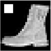
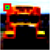
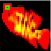
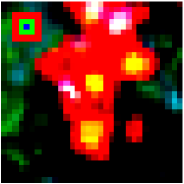
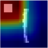
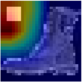
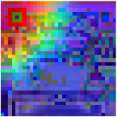
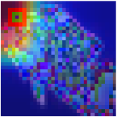
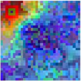
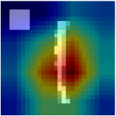
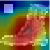
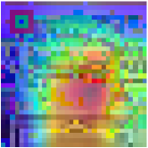
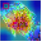
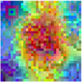
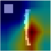
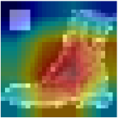
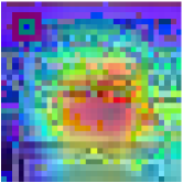
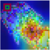
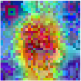
Input Baseline Retrain Ferrari MNIST FMNIST CIFAR-10 CIFAR-20 CIFAR-100

(a) Backdoor Feature Unlearning

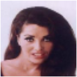
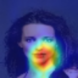
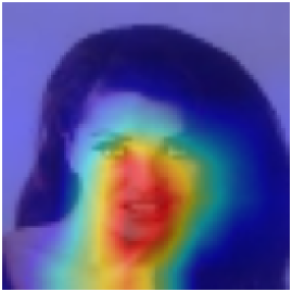
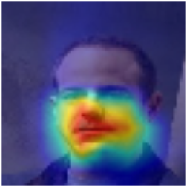
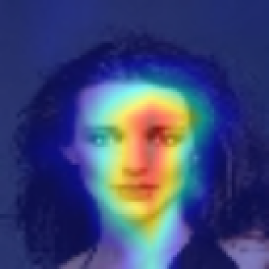
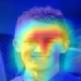
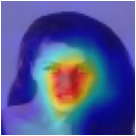
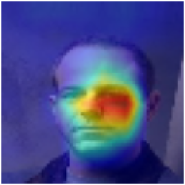
Bias Dataset Unbias Dataset

(b) Biased Feature Unlearning

Figure 5: The attention map of each unlearning method across different unlearning scenarios.

Accuracy

$\mathcal{D}_{r}$ and $\mathcal{D}_{u}$ represent the unbias and bias datasets, respectively. Successful unlearning results in similar accuracies across both datasets ($Acc_{r}\approx Acc_{u}$), ensuring fairness while maintaining high $Acc_{r}$ and $Acc_{u}$ for utility. Tab. 5 shows that the Fine-tune method fails to unlearn bias, as $Acc_{u}$ remains higher than $Acc_{r}$, despite slightly higher $Acc_{r}$ compared to Retrain. FedCDP [66] and FedRecovery [62] exhibit catastrophic forgetting, with low $Acc_{r}$ and $Acc_{u}$, making them unsuitable for biased feature unlearning. In contrast, Ferrari demonstrates effective unlearning with similar $Acc_{r}$ and $Acc_{u}$, and maintains high overall accuracy, indicating successful biased feature unlearning.

Attention Map

Fig. 5(b) shows attention maps analyzing biased feature unlearning. The Baseline model predominantly focuses on the biased feature region (mouth) in both biased and unbiased datasets, suggesting its significant impact on output prediction. However, Ferrari unlearned models redistribute attention across various facial regions in both datasets, similar to the Retrain model. This shift indicates reduced sensitivity to the biased feature, demonstrating successful unlearning. See Appendix A.3.2 for supplementary results.

5.4 Time Efficiency

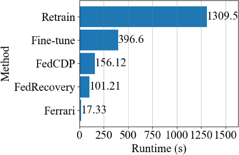
Figure 6: The runtime(s) of each unlearning method.

In Fig. 6, we compare the runtime performance of each unlearning method to demonstrate time efficiency. The Retrain method is expected to have the longest runtime, while Fine-tune is shorter but still slower compared to other methods.

FedCDP [66] and FedRecovery [62] have shorter runtimes Fine-tune method but still longer than Ferrari, mainly due to the need to access training datasets from all clients and the computational expense of gradient residual calculations [62].

In contrast, Ferrari is the fastest method with the shortest runtime, as it only requires access to the local dataset of the unlearn client and achieves feature unlearning by minimizing feature sensitivity within a single epoch.

5.5 Ablation Studies

In this section, we conduct an ablation study to analyze key factors affecting the effectiveness of our proposed Ferrari in Fig. 7: Gaussian noise level($\sigma$), number of $\mathcal{D}_{u}$, and Non-Lipschitz.

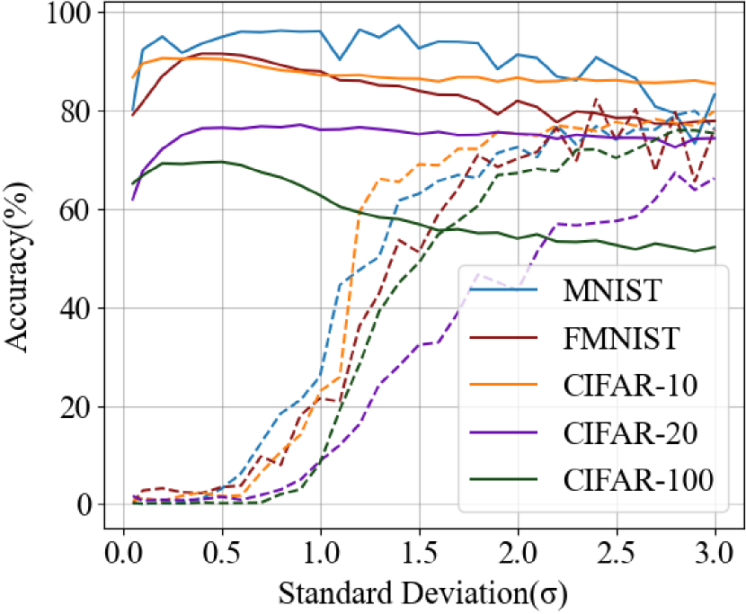
(a) Gaussian noise level($\sigma$)

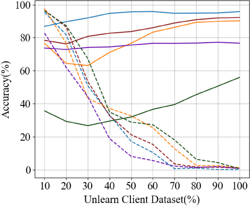
(b) Number of $\mathcal{D}_{u}$

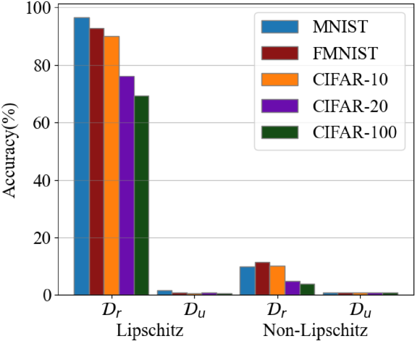
(c) Non-Lipschitz

Figure 7: Ablation studies on Ferrari backdoor feature unlearning. Solid line: $\mathcal{D}_{r}$; dashed line: $\mathcal{D}_{u}$.

Gaussian Noise

The effectiveness of Ferrari is significantly influenced by injected Gaussian noise. Fig. 7(a) shows the accuracy of $\mathcal{D}_{r}$ and $\mathcal{D}_{u}$ across different $\sigma$ levels. In the range $0.05\leq\sigma\leq 1.0$, $\mathcal{D}_{r}$ accuracy stays high and $\mathcal{D}_{u}$ accuracy remains low, indicating a balance. Thus, we implement $\sigma$ values between 0.05 and 1.0 for balanced accuracy across $\mathcal{D}_{r}$ and $\mathcal{D}_{u}$.

Number of Unlearn Dataset

Our analysis, illustrated in Fig. 7(b), demonstrates that Ferrari remains effective with partial $\mathcal{D}_{u}$ from $C_{u}$ for feature unlearning(i.e., data lost). Using 70% of $\mathcal{D}_{u}$ yields comparable accuracy to using 100%, highlighting the method’s flexibility even with partial data.

Non-Lipschitz

We evaluate unlearning performance by removing the denominator in Eq. 6, calling this the non-Lipschitz method, as shown in Fig. 7(c). The results indicate catastrophic forgetting: $\mathcal{D}_{r}$ accuracy drops below 10%, and the unlearned model misclassifies all inputs into a single random class, rendering it useless. This stems from the unbounded loss function in the non-Lipschitz method, unlike the bounded Lipschitz constant in Eq. 6, which provides a theoretical guarantee (see Sec. 4.3).

6 Conclusion

This paper introduces Ferrari, a federated feature unlearning framework designed to efficiently remove sensitive, backdoor, and biased features without extensive retraining. Leveraging Lipschitz continuity, Ferrari reduces model sensitivity to specific features, ensuring robust and fair models. Uniquely, it requires only the participation of the client requesting unlearning, preserving privacy and practicality in FL environments. Experimental results and theoretical analysis demonstrate Ferrari’s effectiveness across various data domains, addressing the crucial need for feature-level unlearning in federated learning. This method also meets regulatory requirements for data deletion while maintaining model performance, thus offering significant value to clients by securing their ’right to be forgotten’ and preventing potential privacy leakage.

Appendix A Appendix

A.1 Proof of Theorem 1

As illustrated in Sec. 3.2, it is hard to build the unlearned data $x^{u}$ for the feature unlearning since adding the perturbation may influence the model accuracy seriously. Suppose the feature is successfully removed when the norm of perturbation is larger than $C$. We define the utility loss $\ell_{1}$ with unlearning feature successfully:

$$\ell_{1}=\min_{\|\delta_{\mathcal{F}}\|\geq C}\mathbb{E}_{(x,y)\in\mathcal{D}}\min_{\theta}\ell\big{(}f_{\theta}(x+\delta_{\mathcal{F}}),y\big{)}$$ (10)

And we define the maximum utility loss with the norm perturbation less than $C$ as:

$$\ell_{2}=\max_{\|\delta_{\mathcal{F}}\|\leq C}\mathbb{E}_{(x,y)\in\mathcal{D}}\min_{\theta}\ell\big{(}f_{\theta}(x+\delta_{\mathcal{F}}),y\big{)}$$ (11)

Assumption 3.

Assume $\ell_{2}\leq\ell_{1}$

Assumption 3 elucidates that the utility loss associated with a perturbation norm less than $C$ is smaller than the utility loss when the perturbation norm is greater than $C$. This assumption is logical, as larger perturbations would naturally lead to greater utility loss.

Assumption 4.

Suppose the federated model achieves zero training loss.

We have the following theorem to elucidate the relation between feature sensitivity removing via Algo. 1 and exact unlearning (see proof in Appendix).

Theorem 2.

If Assumption 3 and 4 hold, the utility loss of unlearned model obtained by Algo. 1 is less than the utility loss with unlearning successfully, i.e.,

$$\ell_{u}\leq\ell_{1},$$ (12)

where $\ell_{u}=\mathbb{E}_{(x,y)\in\mathcal{D}}\big{(}\ell(f_{\theta^{u}}(x),y)$

Proof.

When the unlearning happens during the federated training, the unlearning clients would also optimize the training loss and feature sensitivity simultaneously. Specifically, the optimization process could be written as:

$$\theta_{u}=\operatorname*{arg\,min}_{\theta}\mathbb{E}_{(x,y)\in\mathcal{D}}\big{(}\ell(f_{\theta}(x),y)+\lambda\mathbb{E}_{\delta_{\mathcal{F}}}\frac{\|f_{\theta}(x)-f_{\theta}(x+\delta_{\mathcal{F}})\|_{2}}{\|\delta_{\mathcal{F}}\|_{2}}\big{)},$$

where $\lambda\geq\frac{1}{C}$ is one coefficient. Without loss of generality, we assume the $\ell(f_{\theta}(x),y)=\|f_{\theta}(x)-y)\|$. Denote

$$\Theta^{*}=\operatorname*{arg\,min}_{\theta}\mathbb{E}_{(x,y)\in\mathcal{D}}\ell(f_{\theta}(x),y).$$

If Assumption 4 holds, then $f_{\theta^{*}}(x)=y$ for any $\theta^{*}\in\Theta^{*}$. Therefore, for any $\|\delta_{\mathcal{F}}\|\geq\frac{1}{\lambda}$ such that

$$\begin{split}&\mathbb{E}_{(x,y)\in\mathcal{D}}\big{(}\ell(f_{\theta^{*}}(x),y)+\lambda\mathbb{E}_{\|\delta_{\mathcal{F}}\|\geq\frac{1}{\lambda}}\frac{\|f_{\theta}(x)-f_{\theta^{*}}(x+\delta_{\mathcal{F}})\|_{2}}{\|\delta_{\mathcal{F}}\|_{2}}\big{)}\\ &=\lambda\mathbb{E}_{(x,y)\in\mathcal{D}}\mathbb{E}_{\|\delta_{\mathcal{F}}\|\geq\frac{1}{\lambda}}\frac{\|y-f_{\theta^{*}}(x+\delta_{\mathcal{F}})\|_{2}}{\|\delta_{\mathcal{F}}\|_{2}}\\ &\leq\mathbb{E}_{(x,y)\in\mathcal{D}}\mathbb{E}_{\|\delta_{\mathcal{F}}\|\geq\frac{1}{\lambda}}\|y-f_{\theta^{*}}(x+\delta_{\mathcal{F}})\|_{2}.\end{split}$$ (13)

The last inequality is due to Therefore, we further obtain:

$$\begin{split}\ell_{u}&\leq\min_{\theta\in\mathbb{R}^{d}}\mathbb{E}_{(x,y)\in\mathcal{D}}\big{(}\ell(f_{\theta}(x),y)+\lambda\mathbb{E}_{\|\delta_{\mathcal{F}}\|\geq\frac{1}{\lambda}}\frac{\|f_{\theta}(x)-f_{\theta}(x+\delta_{\mathcal{F}})\|_{2}}{\|\delta_{\mathcal{F}}\|_{2}}\big{)}\\ &\leq\min_{\theta\in\Theta^{*}}\mathbb{E}_{(x,y)\in\mathcal{D}}\big{(}\ell(f_{\theta}(x),y)+\lambda\mathbb{E}_{\|\delta_{\mathcal{F}}\|\geq\frac{1}{\lambda}}\frac{\|f_{\theta}(x)-f_{\theta}(x+\delta_{\mathcal{F}})\|_{2}}{\|\delta_{\mathcal{F}}\|_{2}}\big{)}\\ &\leq\min_{\theta\in\Theta^{*}}\mathbb{E}_{(x,y)\in\mathcal{D}}\mathbb{E}_{\|\delta_{\mathcal{F}}\|\geq\frac{1}{\lambda}}\|y-f_{\theta^{*}}(x+\delta_{\mathcal{F}})\|_{2}\\ &\leq\mathbb{E}_{(x,y)\in\mathcal{D}}\mathbb{E}_{\|\delta_{\mathcal{F}}\|\geq\frac{1}{\lambda}}\min_{\theta\in\Theta^{*}}\|y-f_{\theta^{*}}(x+\delta_{\mathcal{F}})\|_{2}\\ &=\mathbb{E}_{\|\delta_{\mathcal{F}}\|\geq\frac{1}{\lambda}}\mathbb{E}_{(x,y)\in\mathcal{D}}\min_{\theta\in\Theta^{*}}\|y-f_{\theta^{*}}(x+\delta_{\mathcal{F}})\|_{2}\\ &\leq\max_{\|\delta_{\mathcal{F}}\|\geq\frac{1}{\lambda}}\mathbb{E}_{(x,y)\in\mathcal{D}}\min_{\theta\in\mathbb{R}^{d}}\|y-f_{\theta^{*}}(x+\delta_{\mathcal{F}})\|_{2}\\ &\leq\max_{\|\delta_{\mathcal{F}}\|\leq C}\mathbb{E}_{(x,y)\in\mathcal{D}}\min_{\theta\in\mathbb{R}^{d}}\|y-f_{\theta^{*}}(x+\delta_{\mathcal{F}})\|_{2}\\ &=\ell_{2},\end{split}$$ (14)

where the last inequality is due to $\lambda\geq\frac{1}{C}$. According to Assumption 3, we have $\ell_{u}\leq\ell_{1}$

∎

A.2 Experimental Setup

Datasets

MNIST[90]: Both the MNIST[90] and Fashion-MNIST(FMNIST)[92] datasets contain images of handwritten digits and attire, respectively. Each dataset comprises 60,000 training examples and 10,000 test examples. In both datasets, each example is represented as a single-channel image with dimensions of 28x28 pixels, categorized into one of 10 classes. Additionally, the Colored-MNIST(CMNIST)[90] dataset, an extension of the original MNIST, introduces color into the digits of each example. Consequently, images in the Colored MNIST dataset are represented in three channels. CIFAR[93]: The CIFAR-10[93] dataset comprises 60,000 images, each with dimensions of 32x32 pixels and three color channels, distributed across 10 classes. This dataset includes 6,000 images per class and is partitioned into 50,000 training examples and 10,000 test examples. Similarly, the CIFAR-100[93] dataset shares the same image dimensions and structure as CIFAR-10 but extends to 100 classes, with each class containing 600 images. Within each class, there are 500 training images and 100 test images. Moreover, CIFAR-100 organizes its 100 classes into 20 superclasses, forming the CIFAR-20 dataset[93]. CelebA [85]: A face recognition dataset featuring 40 attributes such as gender and facial characteristics, comprising 162,770 training examples and 19,962 test examples. This study will focus on utilizing the CelebA[85] dataset primarily for gender classification tasks.

(a) MNIST

(b) CMNIST

(c) FMNIST

(d) CIFAR-10

(e) CIFAR-20

(f) CIFAR-100

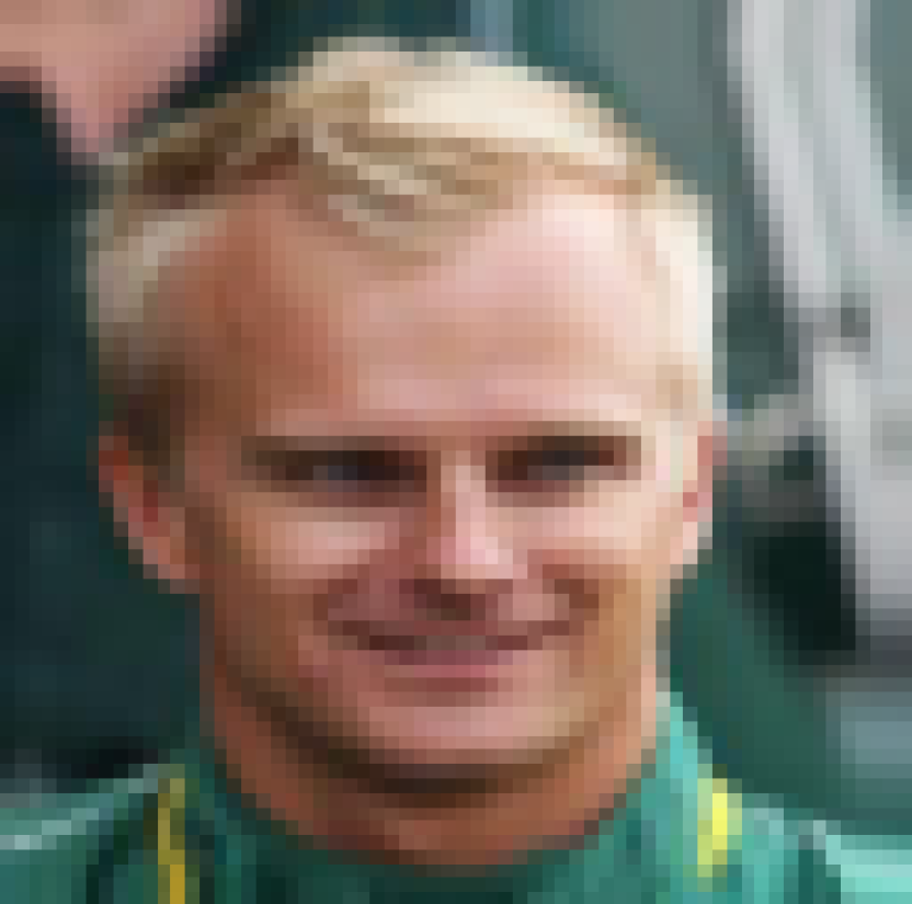
(g) CelebA

Figure 8: Visual representation of dataset samples utilized in this study.

Adult Census Income (Adult)[86] includes 48, 842 records with 14 attributes such as age, gender, education, marital status, etc. The classification task of this dataset is to predict if a person earns over $\$50$K a year based on the census attributes. We then consider marital status as the sensitive feature that aim to unlearn in this study. Diabetes[87] includes 768 personal health records of females at least 21 years old with 8 attributes such as blood pressure, insulin level, age and etc. The classification task of this dataset is to predict if a person has diabetes. We then consider number of pregnancies as the sensitive feature that aim to unlearn in this study.

Baselines

The baseline methods in this study:

Baseline: Original model before unlearning.

Retrain: In scenarios involving sensitive feature unlearning, the retrained model was simply trained using a dataset where Gaussian noise was applied to the unlearned feature region. This approach may lead to performance deterioration, as discussed in Sec. 3.2. For backdoor feature unlearning scenarios, the retrained model was trained using the retain dataset $\mathcal{D}_{r}$, also referred to as the clean dataset. In biased feature unlearning scenarios, the retrained model was trained using a combination of 50% from each of the retain dataset $\mathcal{D}_{r}$ (bias dataset) and the unlearn client local dataset $\mathcal{D}_{u}$ (unbias dataset). This ensures fairness in the model’s performance across both datasets.

Fine-tune: The baseline model is fine-tuned using the retained dataset $\mathcal{D}_{r}$ for 5 epochs. Class-Discriminative Pruning(FedCDP)[66]: A FU framework that achieves class unlearning by utilizing Term Frequency-Inverse Document Frequency (TF-IDF) guided channel pruning, which selectively removes the most discriminative channels related to the target category and followed by fine-tuning without retraining from scratch.

FedRecovery[62]: A FU framework that achieves client unlearning by removing the influence of a client’s data from the global model using a differentially private machine unlearning algorithm that leverages historical gradient submissions without the need for retraining.

A.3 Attention Map

A.3.1 Backdoor Feature Unlearning

Attention map analysis for backdoor samples across model iterations of baseline, retrain, and unlearn model using our proposed Ferrari method on MNIST(Fig. 9), FMNIST(Fig. 10), CIFAR-10(Fig. 11), CIFAR-20(Fig. 12) and CIFAR-100 (Fig. 13)datasets.

Label 1 2 3 4 5 6 7 8 9 Input Baseline Retrain Ferrari

Figure 9: MNIST

Label Trouser Pullover Dress Coat Sandal Shirt Sneaker Bag Boot Input Baseline Retrain Ferrari

Figure 10: FMNIST

Label Car Bird Cat Deer Dog Frog Horse Ship Truck Input Baseline Retrain Ferrari

Figure 11: CIFAR-10

Label Fish Flowers Cont. Fruit Device Furniture Insects Carniv. Synthetic Input Baseline Retrain Ferrari Label Natural Omniv. Medium Inverteb. People Reptiles Small Trees Vehicles Input Baseline Retrain Ferrari

Figure 12: CIFAR-20

Label Fish Baby Bear Beaver Bed Bee Beetle Bicycle Bottle Input Baseline Retrain Ferrari Label Boy Bridge Bus B.fly Camel Can Castle C.plar Cattle Input Baseline Retrain Ferrari Label Chimpz. Clock Cloud C.krch Couch Crab Croc. Cup Dino. Input Baseline Retrain Ferrari Label E.phant F.fish Forest Fox Girl Hamster House K.groo K.board Input Baseline Retrain Ferrari Label Mower Leopard Lion Lizard Lobster Man Mapple M.cycle Mountain Input Baseline Retrain Ferrari Continued on next page

Continued from previous page Label Mushr. Oak Orange. Orchid Otter Palm Pear Pickup Pine Input Baseline Retrain Ferrari Label Plate Poppy Porcp. Possum Rabbit Racc.n Ray Road Rocket Input Baseline Retrain Ferrari Label Sea Seal Shark Shrew Skunk Skyscr. Snail Snake Spider Input Baseline Retrain Ferrari Label Car S.flwer S.pepr Table Tank Phone TV Tiger Tractor Input Baseline Retrain Ferrari Label Trout Tulip Turtle W.drobe Whale Willow TV Woman Worm Input Baseline Retrain Ferrari

Figure 13: CIFAR-100

A.3.2 Biased Feature Unlearning

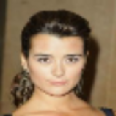
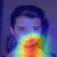
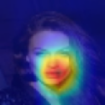
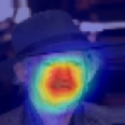
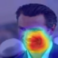
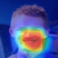
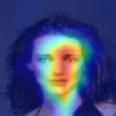
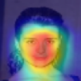
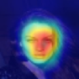
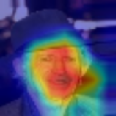
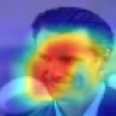
Label Female Male Target Baseline Retrain Ferrari

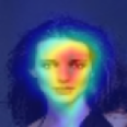
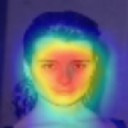
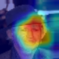
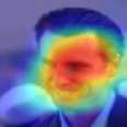
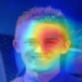
(a) Bias Dataset

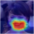
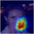
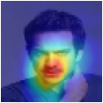
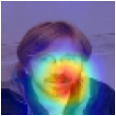
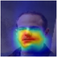
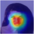
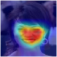
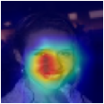
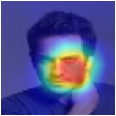
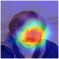
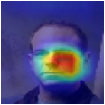
Label Female Male Target Baseline Retrain Ferrari

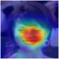
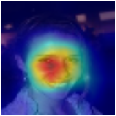
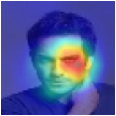
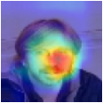
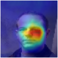
(b) Unbias Dataset

Figure 14: Attention map analysis for bias and unbias samples across model iterations of baseline, retrain, and unlearn model using our proposed Ferrari to unlearn ’mouth’ on CelebA dataset.

A.4 Limitation and Future Work

While our proposed approach of federated feature unlearning demonstrates effectiveness in various unlearning scenarios using only the local dataset of unlearning clients without requiring participation from other clients, thus simulating practical application, it has some inevitable limitations.

The proposed approach necessitates access to the entire dataset from the unlearning client to achieve maximal unlearning effectiveness. However, as demonstrated in Section 5.5, a partial dataset comprising at least 70% of the data yields similar performance to the full dataset. In certain cases, the unlearning client may lose a significant portion of their data, rendering our approach ineffective in such scenarios. Therefore, future work should investigate federated feature unlearning approaches that require only a small portion of the unlearning client’s dataset. Additionally, the proposed approach has only been proven effective for classification models, as it was specifically designed for this purpose. Its effectiveness in other domains, such as generative models, remains to be investigated.

Therefore, future work should explore methods that require only a small portion of the client’s dataset. Additionally, future research will investigate advanced perturbation techniques, support for diverse data types and models, and integration with other privacy-preserving methods to further enhance data protection in FL systems.

References

- [1] J. Konečnỳ, B. McMahan, and D. Ramage, “Federated optimization: Distributed optimization beyond the datacenter,” arXiv preprint arXiv:1511.03575, 2015.
- [2] B. McMahan, E. Moore, D. Ramage, S. Hampson, and B. A. y Arcas, “Communication-efficient learning of deep networks from decentralized data,” in Artificial Intelligence and Statistics, pp. 1273–1282, PMLR, 2017.
- [3] Q. Yang, Y. Liu, T. Chen, and Y. Tong, “Federated machine learning: Concept and applications,” ACM Transactions on Intelligent Systems and Technology (TIST), vol. 10, no. 2, pp. 1–19, 2019.
- [4] E. L. Harding, J. J. Vanto, R. Clark, L. Hannah Ji, and S. C. Ainsworth, “Understanding the scope and impact of the california consumer privacy act of 2018,” Journal of Data Protection & Privacy, vol. 2, no. 3, pp. 234–253, 2019.
- [5] T. Che, Y. Zhou, Z. Zhang, L. Lyu, J. Liu, D. Yan, D. Dou, and J. Huan, “Fast federated machine unlearning with nonlinear functional theory,” in International conference on machine learning, pp. 4241–4268, PMLR, 2023.
- [6] Z. Liu, Y. Jiang, J. Shen, M. Peng, K.-Y. Lam, X. Yuan, and X. Liu, “A survey on federated unlearning: Challenges, methods, and future directions,” 2024.
- [7] N. Romandini, A. Mora, C. Mazzocca, R. Montanari, and P. Bellavista, “Federated unlearning: A survey on methods, design guidelines, and evaluation metrics,” 2024.
- [8] J. Yang and Y. Zhao, “A survey of federated unlearning: A taxonomy, challenges and future directions,” 2023.
- [9] A. Warnecke, L. Pirch, C. Wressnegger, and K. Rieck, “Machine unlearning of features and labels,” in Proc. of the 30th Network and Distributed System Security (NDSS), 2023.
- [10] T. Guo, S. Guo, J. Zhang, W. Xu, and J. Wang, “Efficient attribute unlearning: Towards selective removal of input attributes from feature representations,” 2022.
- [11] T. Guo, S. Guo, J. Zhang, W. Xu, and J. Wang, “Efficient attribute unlearning: Towards selective removal of input attributes from feature representations,” 2022.
- [12] M. Fredrikson, E. Lantz, S. Jha, S. M. Lin, D. Page, and T. Ristenpart, “Privacy in pharmacogenetics: An end-to-end case study of personalized warfarin dosing,” Proceedings of the USENIX Security Symposium. UNIX Security Symposium, vol. 2014, pp. 17–32, 2014.
- [13] M. Fredrikson, S. Jha, and T. Ristenpart, “Model inversion attacks that exploit confidence information and basic countermeasures,” CCS ’15, (New York, NY, USA), p. 1322–1333, Association for Computing Machinery, 2015.
- [14] Y. Zhang, R. Jia, H. Pei, W. Wang, B. Li, and D. Song, “The secret revealer: Generative model-inversion attacks against deep neural networks,” in 2020 IEEE/CVF Conference on Computer Vision and Pattern Recognition (CVPR), pp. 250–258, 2020.
- [15] S. Mehnaz, S. V. Dibbo, E. Kabir, N. Li, and E. Bertino, “Are your sensitive attributes private? novel model inversion attribute inference attacks on classification models,” in USENIX Security Symposium, 2022.
- [16] E. Bagdasaryan, A. Veit, Y. Hua, D. Estrin, and V. Shmatikov, “How to backdoor federated learning,” in Proceedings of the Twenty Third International Conference on Artificial Intelligence and Statistics (S. Chiappa and R. Calandra, eds.), vol. 108 of Proceedings of Machine Learning Research, pp. 2938–2948, PMLR, 26–28 Aug 2020.
- [17] T. D. Nguyen, T. Nguyen, P. L. Nguyen, H. H. Pham, K. D. Doan, and K.-S. Wong, “Backdoor attacks and defenses in federated learning: Survey, challenges and future research directions,” Engineering Applications of Artificial Intelligence, vol. 127, p. 107166, 2024.
- [18] H. Li, C. Wu, S. Zhu, and Z. Zheng, “Learning to backdoor federated learning,” in ICLR 2023 Workshop on Backdoor Attacks and Defenses in Machine Learning, 2023.
- [19] T. Gu, K. Liu, B. Dolan-Gavitt, and S. Garg, “Badnets: Evaluating backdooring attacks on deep neural networks,” IEEE Access, vol. 7, pp. 47230–47244, 2019.
- [20] D. Pessach and E. Shmueli, “A review on fairness in machine learning,” ACM Comput. Surv., vol. 55, feb 2022.
- [21] N. Mehrabi, F. Morstatter, N. Saxena, K. Lerman, and A. Galstyan, “A survey on bias and fairness in machine learning,” ACM Comput. Surv., vol. 54, jul 2021.
- [22] S. Sagawa*, P. W. Koh*, T. B. Hashimoto, and P. Liang, “Distributionally robust neural networks,” in International Conference on Learning Representations, 2020.
- [23] S. Seo, J.-Y. Lee, and B. Han, “Unsupervised learning of debiased representations with pseudo-attributes,” in 2022 IEEE/CVF Conference on Computer Vision and Pattern Recognition (CVPR), pp. 16721–16730, 2022.
- [24] Y. Cao and J. Yang, “Towards making systems forget with machine unlearning,” in 2015 IEEE Symposium on Security and Privacy, pp. 463–480, 2015.
- [25] M. Chen, Z. Zhang, T. Wang, M. Backes, M. Humbert, and Y. Zhang, “When machine unlearning jeopardizes privacy,” in Proceedings of the 2021 ACM SIGSAC Conference on Computer and Communications Security, CCS ’21, (New York, NY, USA), p. 896–911, Association for Computing Machinery, 2021.
- [26] S. Garg, S. Goldwasser, and P. N. Vasudevan, “Formalizing data deletion in the context of the right to be forgotten,” in 39th Annual International Conference on the Theory and Applications of Cryptographic Techniques, Zagreb, Croatia, May 10–14, 2020, Proceedings, vol. 12105 of Lecture Notes in Computer Science, Springer, 2020.
- [27] A. Thudi, H. Jia, I. Shumailov, and N. Papernot, “On the necessity of auditable algorithmic definitions for machine unlearning,” in USENIX Security Symposium, 2021.
- [28] T. T. Nguyen, T. T. Huynh, P. L. Nguyen, A. W.-C. Liew, H. Yin, and Q. V. H. Nguyen, “A survey of machine unlearning,” 2022.
- [29] L. Bourtoule, V. Chandrasekaran, C. A. Choquette-Choo, H. Jia, A. Travers, B. Zhang, D. Lie, and N. Papernot, “Machine unlearning,” in 2021 IEEE Symposium on Security and Privacy (SP), pp. 141–159, 2021.
- [30] H. Yan, X. Li, Z. Guo, H. Li, F. Li, and X. Lin, “Arcane: An efficient architecture for exact machine unlearning,” in Proceedings of the Thirty-First International Joint Conference on Artificial Intelligence, IJCAI-22 (L. D. Raedt, ed.), pp. 4006–4013, International Joint Conferences on Artificial Intelligence Organization, 7 2022. Main Track.
- [31] J. Xu, Z. Wu, C. Wang, and X. Jia, “Machine unlearning: Solutions and challenges,” ArXiv, vol. abs/2308.07061, 2023.
- [32] H. Xu, T. Zhu, L. Zhang, W. Zhou, and P. S. Yu, “Machine unlearning: A survey,” ACM Comput. Surv., vol. 56, aug 2023.
- [33] L. Graves, V. Nagisetty, and V. Ganesh, “Amnesiac machine learning,” in AAAI Conference on Artificial Intelligence, 2020.
- [34] J. Kim and S. S. Woo, “Efficient two-stage model retraining for machine unlearning,” in 2022 IEEE/CVF Conference on Computer Vision and Pattern Recognition Workshops (CVPRW), pp. 4360–4368, 2022.
- [35] S. Lee and S. S. Woo, “Undo: Effective and accurate unlearning method for deep neural networks,” CIKM ’23, (New York, NY, USA), p. 4043–4047, Association for Computing Machinery, 2023.
- [36] M. Chen, W. Gao, G. Liu, K. Peng, and C. Wang, “Boundary unlearning: Rapid forgetting of deep networks via shifting the decision boundary,” in 2023 IEEE/CVF Conference on Computer Vision and Pattern Recognition (CVPR), pp. 7766–7775, 2023.
- [37] T. Shibata, G. Irie, D. Ikami, and Y. Mitsuzumi, “Learning with selective forgetting,” in International Joint Conference on Artificial Intelligence, 2021.
- [38] H. Huang, X. Ma, S. M. Erfani, J. Bailey, and Y. Wang, “Unlearnable examples: Making personal data unexploitable,” in International Conference on Learning Representations, 2021.
- [39] J. Z. Di, J. Douglas, J. Acharya, G. Kamath, and A. Sekhari, “Hidden poison: Machine unlearning enables camouflaged poisoning attacks,” in Workshop on Trustworthy and Socially Responsible Machine Learning, NeurIPS 2022, 2022.
- [40] A. K. Tarun, V. S. Chundawat, M. Mandal, and M. Kankanhalli, “Fast yet effective machine unlearning,” IEEE Transactions on Neural Networks and Learning Systems, pp. 1–10, 2023.
- [41] V. S. Chundawat, A. K. Tarun, M. Mandal, and M. Kankanhalli, “Can bad teaching induce forgetting? unlearning in deep networks using an incompetent teacher,” Proceedings of the AAAI Conference on Artificial Intelligence, vol. 37, pp. 7210–7217, Jun. 2023.
- [42] X. Zhang, J. Wang, N. Cheng, Y. Sun, C. Zhang, and J. Xiao, “Machine unlearning methodology based on stochastic teacher network,” in Advanced Data Mining and Applications (X. Yang, H. Suhartanto, G. Wang, B. Wang, J. Jiang, B. Li, H. Zhu, and N. Cui, eds.), (Cham), pp. 250–261, Springer Nature Switzerland, 2023.
- [43] M. Kurmanji, P. Triantafillou, J. Hayes, and E. Triantafillou, “Towards unbounded machine unlearning,” in Thirty-seventh Conference on Neural Information Processing Systems, 2023.
- [44] Y. Jung, I. Cho, S.-H. Hsu, and J. Hockenmaier, “Attack and reset for unlearning: Exploiting adversarial noise toward machine unlearning through parameter re-initialization,” 2024.
- [45] T. Hoang, S. Rana, S. Gupta, and S. Venkatesh, “Learn to unlearn for deep neural networks: Minimizing unlearning interference with gradient projection,” in Proceedings of the IEEE/CVF Winter Conference on Applications of Computer Vision (WACV), pp. 4819–4828, January 2024.
- [46] A. Abbasi, C. Thrash, E. Akbari, D. Zhang, and S. Kolouri, “Covarnav: Machine unlearning via model inversion and covariance navigation,” 2023.
- [47] D. Choi and D. Na, “Towards machine unlearning benchmarks: Forgetting the personal identities in facial recognition systems,” 2023.
- [48] S. Goel, A. Prabhu, A. Sanyal, S.-N. Lim, P. Torr, and P. Kumaraguru, “Towards adversarial evaluations for inexact machine unlearning,” 2023.
- [49] A. Golatkar, A. Achille, and S. Soatto, “Eternal sunshine of the spotless net: Selective forgetting in deep networks,” in 2020 IEEE/CVF Conference on Computer Vision and Pattern Recognition (CVPR), pp. 9301–9309, 2020.
- [50] A. Golatkar, A. Achille, and S. Soatto, “Forgetting outside the box: Scrubbing deep networks of information accessible from input-output observations,” in Computer Vision – ECCV 2020 (A. Vedaldi, H. Bischof, T. Brox, and J.-M. Frahm, eds.), (Cham), pp. 383–398, Springer International Publishing, 2020.
- [51] A. Golatkar, A. Achille, A. Ravichandran, M. Polito, and S. Soatto, “Mixed-privacy forgetting in deep networks,” in 2021 IEEE/CVF Conference on Computer Vision and Pattern Recognition (CVPR), pp. 792–801, 2021.
- [52] C. Guo, T. Goldstein, A. Hannun, and L. Van Der Maaten, “Certified data removal from machine learning models,” in Proceedings of the 37th International Conference on Machine Learning (H. D. III and A. Singh, eds.), vol. 119 of Proceedings of Machine Learning Research, pp. 3832–3842, PMLR, 13–18 Jul 2020.
- [53] J. Foster, S. Schoepf, and A. Brintrup, “Fast machine unlearning without retraining through selective synaptic dampening,” 2023.
- [54] C. Guo, T. Goldstein, A. Hannun, and L. Van Der Maaten, “Certified data removal from machine learning models,” in Proceedings of the 37th International Conference on Machine Learning (H. D. III and A. Singh, eds.), vol. 119 of Proceedings of Machine Learning Research, pp. 3832–3842, PMLR, 13–18 Jul 2020.
- [55] C. Wu, S. Zhu, and P. Mitra, “Federated unlearning with knowledge distillation,” 2022.
- [56] G. Liu, X. Ma, Y. Yang, C. Wang, and J. Liu, “Federaser: Enabling efficient client-level data removal from federated learning models,” in 2021 IEEE/ACM 29th International Symposium on Quality of Service (IWQOS), pp. 1–10, 2021.
- [57] W. Yuan, H. Yin, F. Wu, S. Zhang, T. He, and H. Wang, “Federated unlearning for on-device recommendation,” in Proceedings of the Sixteenth ACM International Conference on Web Search and Data Mining, WSDM ’23, (New York, NY, USA), p. 393–401, Association for Computing Machinery, 2023.
- [58] X. Cao, J. Jia, Z. Zhang, and N. Z. Gong, “Fedrecover: Recovering from poisoning attacks in federated learning using historical information,” in 2023 IEEE Symposium on Security and Privacy (SP), pp. 1366–1383, 2023.
- [59] X. Gao, X. Ma, J. Wang, Y. Sun, B. Li, S. Ji, P. Cheng, and J. Chen, “Verifi: Towards verifiable federated unlearning,” 2022.
- [60] G. Ye, T. Chen, Q. V. Hung Nguyen, and H. Yin, “Heterogeneous decentralised machine unlearning with seed model distillation,” CAAI Transactions on Intelligence Technology, vol. n/a, no. n/a.
- [61] N. Su and B. Li, “Asynchronous federated unlearning,” in IEEE INFOCOM 2023 - IEEE Conference on Computer Communications, pp. 1–10, 2023.
- [62] L. Zhang, T. Zhu, H. Zhang, P. Xiong, and W. Zhou, “Fedrecovery: Differentially private machine unlearning for federated learning frameworks,” IEEE Transactions on Information Forensics and Security, vol. 18, pp. 4732–4746, 2023.
- [63] A. Halimi, S. Kadhe, A. Rawat, and N. Baracaldo, “Federated unlearning: How to efficiently erase a client in fl?,” 2023.
- [64] G. Li, L. Shen, Y. Sun, Y. Hu, H. Hu, and D. Tao, “Subspace based federated unlearning,” 2023.
- [65] M. Alam, H. Lamri, and M. Maniatakos, “Get rid of your trail: Remotely erasing backdoors in federated learning,” 2023.
- [66] J. Wang, S. Guo, X. Xie, and H. Qi, “Federated unlearning via class-discriminative pruning,” in Proceedings of the ACM Web Conference 2022, WWW ’22, (New York, NY, USA), p. 622–632, Association for Computing Machinery, 2022.
- [67] Y. Zhao, P. Wang, H. Qi, J. Huang, Z. Wei, and Q. Zhang, “Federated unlearning with momentum degradation,” IEEE Internet of Things Journal, pp. 1–1, 2023.
- [68] Y. Liu, L. Xu, X. Yuan, C. Wang, and B. Li, “The right to be forgotten in federated learning: An efficient realization with rapid retraining,” in IEEE INFOCOM 2022 - IEEE Conference on Computer Communications, pp. 1749–1758, 2022.
- [69] A. Dhasade, Y. Ding, S. Guo, A. marie Kermarrec, M. D. Vos, and L. Wu, “Quickdrop: Efficient federated unlearning by integrated dataset distillation,” 2023.
- [70] P. Wang, Z. Yan, M. S. Obaidat, Z. Yuan, L. Yang, J. Zhang, Z. Wei, and Q. Zhang, “Edge caching with federated unlearning for low-latency v2x communications,” IEEE Communications Magazine, pp. 1–7, 2023.
- [71] H. Xia, S. Xu, J. Pei, R. Zhang, Z. Yu, W. Zou, L. Wang, and C. Liu, “Fedme2: Memory evaluation & erase promoting federated unlearning in dtmn,” IEEE Journal on Selected Areas in Communications, vol. 41, no. 11, pp. 3573–3588, 2023.
- [72] S. Moon, S. Cho, and D. Kim, “Feature unlearning for pre-trained gans and vaes,” in AAAI Conference on Artificial Intelligence, 2023.
- [73] S. Bae, S. Kim, H. Jung, and W. Lim, “Gradient surgery for one-shot unlearning on generative model,” 2023.
- [74] Anonymous, “Machine unlearning for image-to-image generative models,” in The Twelfth International Conference on Learning Representations, 2024.
- [75] W. Wang, H. Bai, J. tse Huang, Y. Wan, Y. Yuan, H. Qiu, N. Peng, and M. R. Lyu, “New job, new gender? measuring the social bias in image generation models,” 2024.
- [76] Y. Yao, X. Xu, and Y. Liu, “Large language model unlearning,” 2023.
- [77] C. Yu, S. Jeoung, A. Kasi, P. Yu, and H. Ji, “Unlearning bias in language models by partitioning gradients,” in Findings of the Association for Computational Linguistics: ACL 2023 (A. Rogers, J. Boyd-Graber, and N. Okazaki, eds.), (Toronto, Canada), pp. 6032–6048, Association for Computational Linguistics, July 2023.
- [78] J. Chen and D. Yang, “Unlearn what you want to forget: Efficient unlearning for LLMs,” in Proceedings of the 2023 Conference on Empirical Methods in Natural Language Processing (H. Bouamor, J. Pino, and K. Bali, eds.), (Singapore), pp. 12041–12052, Association for Computational Linguistics, Dec. 2023.
- [79] Y. Yoshida and T. Miyato, “Spectral norm regularization for improving the generalizability of deep learning,” 05 2017.
- [80] A. M. Oberman and J. Calder, “Lipschitz regularized deep neural networks converge and generalize,” CoRR, vol. abs/1808.09540, 2018.
- [81] G. Khromov and S. P. Singh, “Some fundemental aspects about lipschitz continuity of neural networks,” 2023.
- [82] M. Usama and D. E. Chang, “Towards robust neural networks with lipschitz continuity,” in Digital Forensics and Watermarking (C. D. Yoo, Y.-Q. Shi, H. J. Kim, A. Piva, and G. Kim, eds.), (Cham), pp. 373–389, Springer International Publishing, 2019.
- [83] T.-W. Weng, H. Zhang, P.-Y. Chen, J. Yi, D. Su, Y. Gao, C.-J. Hsieh, and L. Daniel, “Evaluating the robustness of neural networks: An extreme value theory approach,” in International Conference on Learning Representations, 2018.
- [84] Y. Yoshida and T. Miyato, “Spectral norm regularization for improving the generalizability of deep learning,” 2017.
- [85] Z. Liu, P. Luo, X. Wang, and X. Tang, “Deep learning face attributes in the wild,” in 2015 IEEE International Conference on Computer Vision (ICCV), pp. 3730–3738, 2015.
- [86] Wenruliu, “Adult income dataset.” Kaggle, 2024.
- [87] M. Akturk, “Diabetes dataset.” Kaggle, 2024.
- [88] Y. Djebrouni, N. Benarba, O. Touat, P. De Rosa, S. Bouchenak, A. Bonifati, P. Felber, V. Marangozova, and V. Schiavoni, “Bias mitigation in federated learning for edge computing,” Proc. ACM Interact. Mob. Wearable Ubiquitous Technol., vol. 7, jan 2024.
- [89] R. Chen, J. Yang, H. Xiong, J. Bai, T. Hu, J. Hao, Y. FENG, J. T. Zhou, J. Wu, and Z. Liu, “Fast model debias with machine unlearning,” in Thirty-seventh Conference on Neural Information Processing Systems, 2023.
- [90] Y. Lecun, L. Bottou, Y. Bengio, and P. Haffner, “Gradient-based learning applied to document recognition,” Proceedings of the IEEE, vol. 86, no. 11, pp. 2278–2324, 1998.
- [91] K. He, X. Zhang, S. Ren, and J. Sun, “Deep residual learning for image recognition,” in 2016 IEEE Conference on Computer Vision and Pattern Recognition (CVPR), pp. 770–778, 2016.
- [92] H. Xiao, K. Rasul, and R. Vollgraf, “Fashion-mnist: a novel image dataset for benchmarking machine learning algorithms,” 2017.
- [93] A. Krizhevsky, “Learning multiple layers of features from tiny images,” 2009.
- [94] R. R. Selvaraju, M. Cogswell, A. Das, R. Vedantam, D. Parikh, and D. Batra, “Grad-cam: Visual explanations from deep networks via gradient-based localization,” in 2017 IEEE International Conference on Computer Vision (ICCV), pp. 618–626, 2017.