The state learner – a super learner for right-censored data

Abstract

In survival analysis, prediction models are needed as stand-alone tools and in applications of causal inference to estimate nuisance parameters. The super learner is a machine learning algorithm which combines a library of prediction models into a meta learner based on cross-validated loss. In right-censored data, the choice of the loss function and the estimation of the expected loss need careful consideration. We introduce the state learner, a new super learner for survival analysis, which simultaneously evaluates libraries of prediction models for the event of interest and the censoring distribution. The state learner can be applied to all types of survival models, works in the presence of competing risks, and does not require a single pre-specified estimator of the conditional censoring distribution. We establish an oracle inequality for the state learner and investigate its performance through numerical experiments. We illustrate the application of the state learner with prostate cancer data, as a stand-alone prediction tool, and, for causal inference, as a way to estimate the nuisance parameter models of a smooth statistical functional.

Keywords: Competing risks, cross-validation, loss based estimation, right-censored data, super learner

1 Introduction

A super learner is a machine learning algorithm that combines a finite set of learners into a meta learner by estimating prediction performance in hold-out samples using a pre-specified loss function [van der Laan et al., 2007]. When the aim is to make a prediction model, super learners combine strong learners, such as Cox regression models and random survival forests [Gerds and Kattan, 2021, Section 8.4]. While the general idea of combining strong learners based on cross-validation stems from earlier work [Wolpert, 1992, Breiman, 1996], the name super learner is justified by an oracle inequality [van der Laan and Dudoit, 2003, van der Vaart et al., 2006].

We define the state learner, a new super learner for right-censored data, which simultaneously estimates the expected loss of learners of the event time distribution and the censoring distribution. The loss function underlying the state learner operates on the coarsened data. In the right-censored survival setting the coarsened data consist of the minimum and the order of the censoring time and the event time as well as the baseline covariates. The state learner can include a broad class of survival models as learners, it can handle competing risks, and it does not require a single pre-specified estimator of the conditional censoring distribution. To analyse the theoretical properties of the state learner we focus on the discrete super learner which combines the library of learners by picking the one that minimises the cross-validated loss [van der Laan et al., 2007]. In the presence of competing risks, our algorithm uses separate libraries of learners for the cumulative hazard functions for each of the competing risks and for the censoring distribution. We show that the oracle selector of the state learner is consistent if all libraries contain a consistent learner and prove a finite sample oracle inequality.

Machine learning based on right-censored data commonly uses the partial log-likelihood as a loss function [e.g., Li et al., 2016, Yao et al., 2017, Lee et al., 2018, Katzman et al., 2018, Gensheimer and Narasimhan, 2019, Lee et al., 2021, Kvamme and Borgan, 2021]. However, this loss function does not work well with data splitting (cross-validation) because the partial log-likelihood loss assigns an infinite value when applied to a test set time point which does not occur in the learning set as soon as the learner predicts piece-wise constant cumulative hazard functions. This is the case for prominent survival learners including the Kaplan-Meier estimator, the random survival forest, and the semi-parametric Cox regression model. When a proportional hazards model is assumed, the baseline hazard function can be profiled out of the likelihood [Cox, 1972]. The cross-validated partial log-likelihood loss [Verweij and van Houwelingen, 1993] has therefore been suggested as a loss function for super learning which however restricts the library of learners to include only Cox proportional hazards models [Golmakani and Polley, 2020].

Alternative approaches for super learning with right-censored data use an inverse probability of censoring weighted (IPCW) loss function [Graf et al., 1999, van der Laan and Dudoit, 2003, Molinaro et al., 2004, Keles et al., 2004, Hothorn et al., 2006, Gerds and Schumacher, 2006, Gonzalez Ginestet et al., 2021], censoring unbiased transformations [Fan and Gijbels, 1996, Steingrimsson et al., 2019], or pseudo-values [Andersen et al., 2003, Mogensen and Gerds, 2013, Sachs et al., 2019]. All these methods rely on an estimator of the censoring distribution, and their drawback is that this estimator has to be pre-specified. An approach which avoids a pre-specified censoring model was proposed independently by Han et al. [2021] and Westling et al. [2021]. In both articles, the authors suggest to iterate between learning of the outcome model and learning of the censoring model using IPCW loss functions. However, no general theoretical guarantees seem to exist for this procedure, and it has not yet been extended to the situation with competing risks.

The state learner algorithm can output a medical risk prediction model [Gerds and Kattan, 2021] which predicts the probability of an event based on covariates in the presence of competing risks. The other application is in targeted learning where conditional event probabilities occur as high-dimensional nuisance parameters which need to be estimated at a certain rate [van der Laan and Rose, 2011, Rytgaard et al., 2021, Rytgaard and van der Laan, 2022]. For the asymptotic bias term of targeted estimator, which uses the state learner to estimate nuisance parameters, we show that a second order product structure holds. We illustrate both applications of the state learner with prostate cancer data [Kattan et al., 2000].

We introduce our notation and framework in Section 2. In Section 3 we define general super learning for right-censored data. Section 4 introduces the state learner, and Section 5 provides theoretical guarantees. In Section 6 we discuss the use of the state learner in the context of targeted learning. We report results of our numerical experiments in Section 7 and analyse a prostate cancer data set in Section 8. Section 9 contains a discussion of the merits and limitations of our proposal. Appendices A and B contain proofs. An implementation of the state learner is available at https://github.com/amnudn/statelearner along with codes for reproducing our numerical experiments.

2 Notation and framework

In a competing risk framework [Andersen et al., 2012], let $T$ be a time to event variable, $D\in\{1,2\}$ the cause of the event, and $X\in\mathcal{X}$ a vector of baseline covariates taking values in a bounded subset $\mathcal{X}\subset\mathbb{R}^{p}$, $p\in\mathbb{N}$. Let $\tau<\infty$ be the prediction horizon. We use $\mathcal{Q}$ to denote the collection of all probability measures on $[0,\tau]\times\{1,2\}\times\mathcal{X}$ such that $(T,D,X)\sim Q$ for some unknown $Q\in\mathcal{Q}$. For $j\in\{1,2\}$, the cause-specific conditional cumulative hazard functions are defined by $\Lambda_{j}\colon[0,\tau]\times\mathcal{X}\rightarrow\mathbb{R}_{+}$ such that

$$\Lambda_{j}(t\mid x)=\int_{0}^{t}\frac{Q(T\in\mathop{}\!\mathrm{d}s,D=j\mid X=x)}{Q(T\geq s\mid X=x)}.$$

For ease of presentation we assume throughout that the map $t\mapsto\Lambda_{j}(t\mid x)$ is continuous for all $x$ and $j$. This is not a limitation: All arguments carry over directly to the general case. We denote by $S$ the conditional event-free survival function:

$$S(t\mid x)=\exp\left\{-\Lambda_{1}(t\mid x)-\Lambda_{2}(t\mid x)\right\}.$$ (1)

Let $\mathcal{M}_{\tau}$ denote the space of all conditional cumulative hazard functions on $[0,\tau]\times\mathcal{X}$. Any distribution $Q\in\mathcal{Q}$ can be characterised by

$$\begin{split}Q(\mathop{}\!\mathrm{d}t,j,\mathop{}\!\mathrm{d}x)=&\left\{S(t-\mid x)\Lambda_{1}(\mathop{}\!\mathrm{d}t\mid x)H(\mathop{}\!\mathrm{d}x)\right\}^{\mathds{1}{\{j=1\}}}\\ &\left\{S(t-\mid x)\Lambda_{2}(\mathop{}\!\mathrm{d}t\mid x)H(\mathop{}\!\mathrm{d}x)\right\}^{\mathds{1}{\{j=2\}}},\end{split}$$

where $\Lambda_{j}\in\mathcal{M}_{\tau}$ for $j=1,2$ and $H$ is the marginal distribution of the covariates.

We consider the right-censored setting in which we observe the coarsened data $O=(\tilde{T},\tilde{D},X)$, where $\tilde{T}=\min(T,C)$ for a right-censoring time $C$, $\Delta=\mathds{1}{\{T\leq C\}}$, and $\tilde{D}=\Delta D$. Let $\mathcal{P}$ denote a set of probability measures on the sample space $\mathcal{O}=[0,\tau]\times\{0,1,2\}\times\mathcal{X}$ such that $O\sim P$ for some unknown $P\in\mathcal{P}$. We assume that the event times and the censoring times are conditionally independent given covariates, $T\mathchoice{\mathrel{\hbox to0.0pt{$\displaystyle\perp$\hss}\mkern 2.0mu{\displaystyle\perp}}}{\mathrel{\hbox to0.0pt{$\textstyle\perp$\hss}\mkern 2.0mu{\textstyle\perp}}}{\mathrel{\hbox to0.0pt{$\scriptstyle\perp$\hss}\mkern 2.0mu{\scriptstyle\perp}}}{\mathrel{\hbox to0.0pt{$\scriptscriptstyle\perp$\hss}\mkern 2.0mu{\scriptscriptstyle\perp}}}C\mid X$. This implies that any distribution $P\in\mathcal{P}$ is characterised by a distribution $Q\in\mathcal{Q}$ and a conditional cumulative hazard function for $C$ given $X$ [c.f., Begun et al., 1983, Gill et al., 1997]. We use $\Gamma\in\mathcal{M}_{\tau}$ to denote the conditional cumulative hazard function for censoring. For ease of presentation we now also assume that $\Gamma(\makebox[4.30554pt]{{$\cdot$}}\mid x)$ is continuous for all $x$. We let $(t,x)\mapsto G(t\mid x)=\exp\left\{-\Gamma(t\mid x)\right\}$ denote the survival function of the conditional censoring distribution. The distribution $P$ is characterised by

$$\begin{split}P(\mathop{}\!\mathrm{d}t,j,\mathop{}\!\mathrm{d}x)=&\left\{G(t-\mid x)S(t-\mid x)\Lambda_{1}(\mathop{}\!\mathrm{d}t\mid x)H(\mathop{}\!\mathrm{d}x)\right\}^{\mathds{1}{{\{j=1\}}}}\\ &\left\{G(t-\mid x)S(t-\mid x)\Lambda_{2}(\mathop{}\!\mathrm{d}t\mid x)H(\mathop{}\!\mathrm{d}x)\right\}^{\mathds{1}{{\{j=2\}}}}\\ &\left\{G(t-\mid x)S(t-\mid x)\Gamma(\mathop{}\!\mathrm{d}t\mid x)H(\mathop{}\!\mathrm{d}x)\right\}^{\mathds{1}{{\{j=0\}}}}\\ =&\left\{G(t-\mid x)Q(\mathop{}\!\mathrm{d}t,j,\mathop{}\!\mathrm{d}x)\right\}^{\mathds{1}{{\{j\neq 0\}}}}\\ &\left\{G(t-\mid x)S(t-\mid x)\Gamma(\mathop{}\!\mathrm{d}t\mid x)H(\mathop{}\!\mathrm{d}x)\right\}^{\mathds{1}{{\{j=0\}}}}.\end{split}$$ (2)

Hence, we may write $\mathcal{P}=\{P_{Q,\Gamma}:Q\in\mathcal{Q},\Gamma\in\mathcal{G}\}$ for some $\mathcal{G}\subset\mathcal{M}_{\tau}$. We also have $H$-almost everywhere

$$P(\tilde{T}>t\mid X=x)=S(t\mid x)G(t\mid x)=\exp\left\{-\Lambda_{1}(t\mid x)-\Lambda_{2}(t\mid x)-\Gamma(t\mid x)\right\}.$$

We further assume that there exists $\kappa<\infty$ such that $\Lambda_{j}(\tau-\mid x)<\kappa$, for $j\in\{1,2\}$, and $\Gamma(\tau-\mid x)<\kappa$ for almost all $x\in\mathcal{X}$. Note that this implies that $G(\tau-\mid x)$ is bounded away from zero for almost all $x\in\mathcal{X}$. Under these assumptions, the conditional cumulative hazard functions $\Lambda_{j}$ and $\Gamma$ can be identified from $P$ by

$$\Lambda_{j}(t\mid x) =\int_{0}^{t}\frac{P(\tilde{T}\in\mathop{}\!\mathrm{d}s,\tilde{D}=j\mid X=x)}{P(\tilde{T}\geq s\mid X=x)},$$ (3)

$$\Gamma(t\mid x) =\int_{0}^{t}\frac{P(\tilde{T}\in\mathop{}\!\mathrm{d}s,\tilde{D}=0\mid X=x)}{P(\tilde{T}\geq s\mid X=x)}.$$ (4)

Thus, we can consider $\Lambda_{j}$ and $\Gamma$ as operators which map from $\mathcal{P}$ to $\mathcal{M}_{\tau}$.

3 The concept of super learning

In survival analysis, a super learner can be used to estimate a parameter $\Psi$ which can be identified from the observed data distribution $P\in\mathcal{P}$. In this section, to introduce the discrete super learner and the oracle learner, we consider estimation of the function-valued parameter $\Psi:\mathcal{P}\to\mathcal{M}_{\tau}$, given by $\Psi(P)=\Lambda_{j}$. This parameter is identified via equation (3) on $[0,\tau]$.

As input to the super learner we need a data set $\mathcal{D}_{n}=\{O_{i}\}_{i=1}^{n}$ of i.i.d. observations from $P\in\mathcal{P}$ and a collection of candidate learners $\mathcal{A}$. Each learner $a\in\mathcal{A}$ is a map $a\colon\mathcal{O}^{n}\rightarrow\mathcal{M}_{\tau}$ which takes a data set as input and returns an estimate $a(\mathcal{D}_{n})\in\mathcal{M}_{\tau}$ of $\Lambda_{j}$. In what follows, we use the short-hand notation $P[f]=\int f(o)P(\mathop{}\!\mathrm{d}o)$. A super learner evaluates the performance of $a\in\mathcal{A}$ with a loss function $L\colon\mathcal{M}_{\tau}\times\mathcal{O}\rightarrow\mathbb{R}_{+}$ and estimates the expected loss $P[L(a(\mathcal{D}_{n}),\makebox[4.30554pt]{{$\cdot$}})]$ using cross-validation. Specifically, the expected loss of $a\in\mathcal{A}$ is estimated by splitting the data set $\mathcal{D}_{n}$ into $K$ disjoint approximately equally sized subsets $\mathcal{D}_{n}^{1},\mathcal{D}_{n}^{2},\dots,\mathcal{D}_{n}^{K}$ and then calculating the cross-validated loss

$$\hat{R}_{n}(a;L)=\frac{1}{K}\sum_{k=1}^{K}\frac{1}{|\mathcal{D}_{n}^{k}|}\sum_{O_{i}\in\mathcal{D}_{n}^{k}}L{\left(a{(\mathcal{D}_{n}^{-k})},O_{i}\right)},\quad\text{with}\quad\mathcal{D}_{n}^{-k}=\mathcal{D}_{n}\setminus\mathcal{D}_{n}^{k}.$$

The subset $\mathcal{D}_{n}^{-k}$ is referred to as the $k$’th training sample, while $\mathcal{D}_{n}^{k}$ is referred to as the $k$’th test or hold-out sample. The discrete super learner is defined as

$$\hat{a}_{n}=\operatorname*{\arg\!\min}_{a\in\mathcal{A}}\hat{R}_{n}(a;L).$$

The oracle learner is defined as the learner that minimises the expected loss under the data-generating distribution $P$, i.e.,

$$\tilde{a}_{n}=\operatorname*{\arg\!\min}_{a\in\mathcal{A}}\tilde{R}_{n}(a;L),\quad\text{with}\quad\tilde{R}_{n}(a;L)=\frac{1}{K}\sum_{k=1}^{K}P{\left[L{\left(a{(\mathcal{D}_{n}^{-k})},\makebox[4.30554pt]{{$\cdot$}}\right)}\right]}.$$

Note that both the discrete super learner and the oracle learner depend on the library of learners and on the number of folds $K$, and that the oracle learner is a function of the data and the unknown data-generating distribution. However, these dependencies are suppressed in the notation.

4 The state learner

The main idea of the state learner is to jointly use learners for $\Lambda_{1}$, $\Lambda_{2}$, and $\Gamma$, and the relations in equation (2), to learn a feature of the observed data distribution $P$. The discrete state learner ranks a tuple of learners for the tuple of the cumulative hazard functions $(\Lambda_{1},\Lambda_{2},\Gamma)$ based on how well they jointly model the observed data. Risk predictions can then be obtained by combining $\Lambda_{1}$ and $\Lambda_{2}$ from the highest ranked tuple using a well-known formula [Benichou and Gail, 1990, Ozenne et al., 2017]. To formally introduce the state learner, we define the multi-state process

$$\eta(t)=\mathds{1}\{\tilde{T}\leq t,\tilde{D}=1\}+2\,\mathds{1}\{\tilde{T}\leq t,\tilde{D}=2\}-\mathds{1}\{\tilde{T}\leq t,\tilde{D}=0\},\quad\text{for}\quad t\in[0,\tau].$$

At time $t$, we observe that each individual is in one of four mutually exclusive states: $0$, $1$, $2$, or $-1$. The conditional distribution of the process $\eta(t)$ given baseline covariates $X$ is determined by the function

$$F(t,k,x)=P(\eta(t)=k\mid X=x),\quad\text{for all}\quad t\in[0,\tau],k\in\{-1,0,1,2\},x\in\mathcal{X}.$$ (5)

The function $F$ describes the conditional state occupation probabilities of the multi-state process $\eta$. We construct a super learner for $F$. The target of this super learner is the function-valued parameter $\Psi(P)=F$ which is identified through equation (5). Under conditional independent censoring each quadruple $(\Lambda_{1},\Lambda_{2},\Gamma,H)$ characterises a distribution $P\in\mathcal{P}$, c.f. equation (2), which in turn determines $(F,H)$. Hence, a learner for $F$ can be constructed from learners for $\Lambda_{1}$, $\Lambda_{2}$, and $\Gamma$ as follows:

$$\begin{split}F(t,0,x)&=P(\tilde{T}>t\mid X=x)=\exp{{\{-\Lambda_{1}(t\mid x)-\Lambda_{2}(t\mid x)-\Gamma(t\mid x)\}}},\\ F(t,1,x)&=P(\tilde{T}\leq t,\tilde{D}=1\mid X=x)=\int_{0}^{t}F(s-,0,x)\Lambda_{1}(\mathop{}\!\mathrm{d}s\mid x),\\ F(t,2,x)&=P(\tilde{T}\leq t,\tilde{D}=2\mid X=x)=\int_{0}^{t}F(s-,0,x)\Lambda_{2}(\mathop{}\!\mathrm{d}s\mid x),\\ F(t,-1,x)&=P(\tilde{T}\leq t,\tilde{D}=0\mid X=x)=\int_{0}^{t}F(s-,0,x)\Gamma(\mathop{}\!\mathrm{d}s\mid x).\end{split}$$ (6)

The state learner requires three libraries of learners (c.f., Section 3), $\mathcal{A}_{1}$, $\mathcal{A}_{2}$, and $\mathcal{B}$, where $\mathcal{A}_{1}$ and $\mathcal{A}_{2}$ contain learners for the conditional cause-specific cumulative hazard functions $\Lambda_{1}$ and $\Lambda_{2}$, respectively, and $\mathcal{B}$ contains learners for the conditional cumulative hazard function of the censoring distribution. Based on the Cartesian product of libraries of learners for $(\Lambda_{1},\Lambda_{2},\Gamma)$ we construct a library $\mathcal{F}$ of learners for $F$:

$$\mathcal{F}(\mathcal{A}_{1},\mathcal{A}_{2},\mathcal{B}) =\{\varphi_{a_{1},a_{2},b}:a_{1}\in\mathcal{A}_{1},a_{2}\in\mathcal{A}_{2},b\in\mathcal{B}\},$$

where in correspondence with the relations in equation (6),

$$\varphi_{a_{1},a_{2},b}(\mathcal{D}_{n})(t,0,x) =\exp{\{-a_{1}(\mathcal{D}_{n})(s\mid x)-a_{2}(\mathcal{D}_{n})(s\mid x)-b(\mathcal{D}_{n})(s\mid x)\}},$$

$$\varphi_{a_{1},a_{2},b}(\mathcal{D}_{n})(t,1,x) =\int_{0}^{t}\varphi_{a_{1},a_{2},b}(\mathcal{D}_{n})(s-,0,x)a_{1}(\mathcal{D}_{n})(\mathop{}\!\mathrm{d}s\mid x),$$

$$\varphi_{a_{1},a_{2},b}(\mathcal{D}_{n})(t,2,x) =\int_{0}^{t}\varphi_{a_{1},a_{2},b}(\mathcal{D}_{n})(s-,0,x)a_{2}(\mathcal{D}_{n})(\mathop{}\!\mathrm{d}s\mid x),$$

$$\varphi_{a_{1},a_{2},b}(\mathcal{D}_{n})(t,-1,x) =\int_{0}^{t}\varphi_{a_{1},a_{2},b}(\mathcal{D}_{n})(s-,0,x)b(\mathcal{D}_{n})(\mathop{}\!\mathrm{d}s\mid x).$$

To evaluate how well a function $F$ predicts the observed multi-state process we use the integrated Brier score $\bar{B}_{\tau}(F,O)=\int_{0}^{\tau}B_{t}(F,O)\mathop{}\!\mathrm{d}t$, where $B_{t}$ is the Brier score [Brier et al., 1950] at time $t\in[0,\tau]$,

$$B_{t}(F,O)=\sum_{j=-1}^{2}\left(F(t,j,X)-\mathds{1}{\{\eta(t)=j\}}\right)^{2}.$$

Based on a split of a data set $\mathcal{D}_{n}$ into $K$ disjoint approximately equally sized subsets (see Section 3), each learner $\varphi_{a_{1},a_{2},b}$ in the library $\mathcal{F}(\mathcal{A}_{1},\mathcal{A}_{2},\mathcal{B})$ is evaluated using the cross-validated loss,

$$\hat{R}_{n}(\varphi_{a_{1},a_{2},b};\bar{B}_{\tau})=\frac{1}{K}\sum_{k=1}^{K}\frac{1}{|\mathcal{D}_{n}^{k}|}\sum_{O_{i}\in\mathcal{D}_{n}^{k}}\bar{B}_{\tau}{\left(\varphi_{a_{1},a_{2},b}{(\mathcal{D}_{n}^{-k})},O_{i}\right)},$$

and the discrete state learner is given by

$$\hat{\varphi}_{n} =\operatorname*{\arg\!\min}_{(a_{1},a_{2},b)\in\mathcal{A}_{1}\times\mathcal{A}_{2}\times\mathcal{B}}\hat{R}_{n}(\varphi_{a_{1},a_{2},b};\bar{B}_{\tau}).$$

5 Theoretical results for the state learner

In this section we establish theoretical guarantees for the state learner. We show that the state learner is consistent if its library contains a consistent learner, and we establish a finite sample inequality for the excess risk of the state learner compared to the oracle. Finally we show that a certain second order structure is preserved when the state learner is used for targeted learning.

5.1 Consistency

Proposition 1 can be derived from the fact that the integrated Brier score (also called the continuous ranked probability score) is a strictly proper scoring rule [Gneiting and Raftery, 2007]. This implies that if we minimise the average loss of the integrated Brier score, we recover the parameters of the data-generating distribution. Specifically, this implies that the oracle of a state learner is consistent if the library of learners contains at least one learner that is consistent for estimation of $F$. Recall that the function $F$ implicitly depends on the data-generating probability measure $P\in\mathcal{P}$ but that this was suppressed in the notation. We now make this dependence explicit by writing $F_{0}$ for the function which is obtained by substituting a specific $P_{0}\in\mathcal{P}$ for $P$ in equation (6). In the following we let $\mathcal{H}_{\mathcal{P}}=\{F_{P}:P\in\mathcal{P}\}$ where $F_{P}$ is defined as in equation (5) using the measure $P\in\mathcal{P}$.

Proposition 1.

If $P_{0}\in\mathcal{P}$ then

$$F_{0}=\operatorname*{\arg\!\min}_{F\in\mathcal{H}_{\mathcal{P}}}P_{0}{[\bar{B}_{\tau}(F,\makebox[4.30554pt]{{$\cdot$}})]},$$

$H$-almost surely for any $j\in\{-1,0,1,2\}$ and almost any $t\in[0,\tau]$.

Proof.

See Appendix A. ∎

5.2 Oracle inequalities

We establish a finite sample oracle result for the state learner. Our Corollary 1 is in essence a special case of Theorem 2.3 in [van der Vaart et al., 2006]. We assume that we split the data into equally sized folds, and for simplicity of presentation we take $n$ to be such that $|\mathcal{D}_{n}^{-k}|=n/K$ with $K$ fixed. We will allow the number of learners to grow with $n$ and write $\mathcal{F}_{n}=\mathcal{F}(\mathcal{A}_{1,n},\mathcal{A}_{2,n},\mathcal{B}_{n})$ as short-hand notation and to emphasise the dependence on $n$. In the following we let the space $\mathcal{H}_{\mathcal{P}}$ be equipped with the norm $\|\makebox[4.30554pt]{{$\cdot$}}\|_{P_{0}}$ defined as

$$\|F\|_{P_{0}}=\left\{\sum_{j=-1}^{2}\int_{\mathcal{X}}\int_{0}^{\tau}F(t,j,x)^{2}\mathop{}\!\mathrm{d}tH_{0}(\mathop{}\!\mathrm{d}x)\right\}^{1/2}.$$ (7)

Corollary 1.

For all $P_{0}\in\mathcal{P}$, $n\in\mathbb{N}$, $k\in\{1,\dots,K\}$, and $\delta>0$,

$$\operatorname{\mathbb{E}}_{P_{0}}{\left[\|\hat{\varphi}_{n}(\mathcal{D}_{n}^{-k})-F_{0}\|_{P_{0}}^{2}\right]} \leq(1+2\delta)\operatorname{\mathbb{E}}_{P_{0}}{\left[\|\tilde{\varphi}_{n}(\mathcal{D}_{n}^{-k})-F_{0}\|_{P_{0}}^{2}\right]}$$

$$\quad+(1+\delta)16K\tau\left(13+\frac{12}{\delta}\right)\frac{\log(1+|\mathcal{F}_{n}|)}{n}.$$

Proof.

See Appendix A. ∎

Corollary 1 has the following asymptotic consequences.

Corollary 2.

Assume that $|\mathcal{F}_{n}|=\textit{O}(n^{q})$, for some $q\in\mathbb{N}$ and that there exists a sequence $\varphi_{n}\in\mathcal{F}_{n}$, $n\in\mathbb{N}$, such that $\operatorname{\mathbb{E}}_{P_{0}}{\left[\|\varphi_{n}(\mathcal{D}_{n}^{-k})-F_{0}\|_{P_{0}}^{2}\right]}=\textit{O}(n^{-\alpha})$, for some $\alpha\leq 1$.

1. If $\alpha=1$ then $\operatorname{\mathbb{E}}_{P_{0}}{\left[\|\hat{\varphi}_{n}(\mathcal{D}_{n}^{-k})-F_{0}\|_{P_{0}}^{2}\right]}=\textit{O}(\log(n)n^{-1})$.

2. If $\alpha<1$ then $\operatorname{\mathbb{E}}_{P_{0}}{\left[\|\hat{\varphi}_{n}(\mathcal{D}_{n}^{-k})-F_{0}\|_{P_{0}}^{2}\right]}=\textit{O}(n^{-\alpha})$.

Proof.

See Appendix A. ∎

5.3 Transience of the second order remainder structure

In this section we demonstrate a theoretical property of the state learner which is useful for targeted learning (c.f., Section 6). Specifically we consider an estimator of a target parameter which is obtained by substituting the state learner estimates of the nuisance parameters $\Lambda_{1}$, $\Lambda_{2}$, and $\Gamma$. An example is an estimator of the cumulative incidence curve, which can be obtained from estimators of $\Lambda_{1}$ and $\Lambda_{2}$. Another example is provided in Section 6. By equations (3) and (4) and the definition of $F$, we have

$$\Gamma(t,x)=\int_{0}^{t}\frac{F(\mathop{}\!\mathrm{d}s,-1,x)}{F(s-,0,x)},\quad\text{and}\quad\Lambda_{j}(t,x)=\int_{0}^{t}\frac{F(\mathop{}\!\mathrm{d}s,j,x)}{F(s-,0,x)},\quad j\in\{1,2\},$$ (8)

and thus an estimator based on $\hat{\Lambda}_{1,n}$, $\hat{\Lambda}_{2,n}$, and $\hat{\Gamma}_{n}$ can also be obtained from an estimator of $F$ using equation (8). A so-called targeted estimator has the key feature that it is asymptotically equivalent to a sum of i.i.d. random variables plus a second order remainder term [van der Laan and Rose, 2011, Hines et al., 2022]. For the setting with competing risks, the remainder term is dominated by terms of the form

$$P{\left[\int_{0}^{\tau}w_{n}(s,\makebox[4.30554pt]{{$\cdot$}})\hat{M}_{1,n}(s\mid\makebox[4.30554pt]{{$\cdot$}})\hat{M}_{2,n}(\mathop{}\!\mathrm{d}s\mid\makebox[4.30554pt]{{$\cdot$}})\right]},$$ (9)

where $(\hat{M}_{1,n},\hat{M}_{2,n})$ is any of the nine combinations of $\hat{M}_{1,n}\in\{[\Gamma-\hat{\Gamma}_{n}],[\Lambda_{1}-\hat{\Lambda}_{1,n}],[\Lambda_{2}-\hat{\Lambda}_{2,n}]\}$ and $\hat{M}_{2,n}\in\{[\Gamma-\hat{\Gamma}_{n}],[\Lambda_{1}-\hat{\Lambda}_{1,n}],[\Lambda_{2}-\hat{\Lambda}_{2,n}]\}$, and $w_{n}$ is some data-dependent function with domain $[0,\tau]\times\mathcal{X}$ [van der Laan and Robins, 2003]. In particular, a targeted estimator will be asymptotically linear if the ‘products’ of the estimation errors $\hat{M}_{1,n}$ and $\hat{M}_{2,n}$ in equation (9) are $\textit{o}_{P}{(n^{-1/2})}$. Proposition 2 states that if equation (9) holds for a targeted estimator based on estimators $\hat{\Lambda}_{1,n}$, $\hat{\Lambda}_{2,n}$, and $\hat{\Gamma}_{n}$, then a similar product structure holds for a targeted estimator based on $\hat{F}_{n}$. We state the result for the special case that $\hat{M}_{1,n}=\Gamma-\hat{\Gamma}_{n}$ and $\hat{M}_{2,n}=\Lambda_{1}-\hat{\Lambda}_{1,n}$, but similar results hold for any combinations of $\Gamma-\hat{\Gamma}_{n}$, $\Lambda_{1}-\hat{\Lambda}_{1,n}$, and $\Lambda_{2}-\hat{\Lambda}_{2,n}$.

Proposition 2.

Assume that $w(s,x)\leq c$, $F(s,0,x)\geq 1/c$ and $\hat{F}_{n}(s,0,x)\geq 1/c$ for some $c>0$ for all $s\in[0,\tau]$ and $x\in\mathcal{X}$. Then there are real-valued uniformly bounded functions $w^{a}_{n}$, $w^{b}_{n}$, $w^{c}_{n}$, and $w^{d}_{n}$ with domain $[0,\tau]^{2}\times\mathcal{X}$ such that

$$P_{0}{\left[\int_{0}^{\tau}w(s,\makebox[4.30554pt]{{$\cdot$}})\left\{\Gamma_{0}(s,\makebox[4.30554pt]{{$\cdot$}})-\hat{\Gamma}_{n}(s,\makebox[4.30554pt]{{$\cdot$}})\right\}[\Lambda_{0}-\hat{\Lambda}_{n}](\mathop{}\!\mathrm{d}s,\makebox[4.30554pt]{{$\cdot$}})\right]}$$

$$=P_{0}{\left[\int_{0}^{\tau}\int_{0}^{s}w^{a}_{n}(s,u,\makebox[4.30554pt]{{$\cdot$}})[F_{0}-\hat{F}_{n}](u-,0,\makebox[4.30554pt]{{$\cdot$}})[F_{0}-\hat{F}_{n}](s-,0,\makebox[4.30554pt]{{$\cdot$}})F_{0}(\mathop{}\!\mathrm{d}u,2,\makebox[4.30554pt]{{$\cdot$}})F_{0}(\mathop{}\!\mathrm{d}s,1,\makebox[4.30554pt]{{$\cdot$}})\right]}$$

$$\quad+P_{0}{\left[\int_{0}^{\tau}\int_{0}^{s}w^{b}_{n}(s,u,\makebox[4.30554pt]{{$\cdot$}})[F_{0}-\hat{F}_{n}](u-,0,\makebox[4.30554pt]{{$\cdot$}})F_{0}(\mathop{}\!\mathrm{d}u,2,\makebox[4.30554pt]{{$\cdot$}})[F_{0}-\hat{F}_{n}](\mathop{}\!\mathrm{d}s,1,\makebox[4.30554pt]{{$\cdot$}})\right]}$$

$$\quad+P_{0}{\left[\int_{0}^{\tau}\int_{0}^{s}w^{c}_{n}(s,u,\makebox[4.30554pt]{{$\cdot$}})[F_{0}-\hat{F}_{n}](\mathop{}\!\mathrm{d}u,2,\makebox[4.30554pt]{{$\cdot$}})[F_{0}-\hat{F}_{n}](s-,0,\makebox[4.30554pt]{{$\cdot$}})F_{0}(\mathop{}\!\mathrm{d}s,1,\makebox[4.30554pt]{{$\cdot$}})\right]}$$

$$\quad+P_{0}{\left[\int_{0}^{\tau}\int_{0}^{s}w^{d}_{n}(s,u,\makebox[4.30554pt]{{$\cdot$}})[F_{0}-\hat{F}_{n}](\mathop{}\!\mathrm{d}u,2,\makebox[4.30554pt]{{$\cdot$}})[F_{0}-\hat{F}_{n}](\mathop{}\!\mathrm{d}s,1,\makebox[4.30554pt]{{$\cdot$}})\right]}.$$

Proof.

See Appendix B. ∎

6 Targeted learning

In this section, we consider a suitably smooth operator $\theta\colon\mathcal{Q}\rightarrow\Theta$ which represents a target parameter of interest. The parameter space $\Theta$ can be a subset of $\mathbb{R}^{d}$ or a subset of a function space, for example a subset of $\mathcal{M}_{\tau}$ as in Section 3. In subsection 6.1 we discuss an example from causal inference where $\theta$ is the average treatment effect and $\Theta=[-1,1]$. To discuss the role of the state learner for targeted learning we briefly review some results from semiparametric efficiency theory. Extensive reviews and introductions are available elsewhere [e.g., Pfanzagl and Wefelmeyer, 1982, Bickel et al., 1993, van der Laan and Robins, 2003, Tsiatis, 2007, Kennedy, 2016]. Under the assumption of conditional independent censoring and positivity, $\theta$ is identifiable from $\mathcal{P}$ which means that there exists an operator $\Psi\colon\mathcal{P}\rightarrow\Theta$ such that $\theta(Q)=\Psi(P_{Q,\Gamma})$ for all $\Gamma\in\mathcal{M}_{\tau}$. By equation (2) this implies that we may write

$$\theta(Q)=\Psi(P)=\tilde{\Psi}^{0}(\Lambda_{1},\Lambda_{2},H),$$

for some operator $\tilde{\Psi}^{0}$. The state learner provides a ranking of all tuples $(a_{1},a_{2},b)\in\mathcal{A}_{1}\times\mathcal{A}_{2}\times\mathcal{B}$. We use $\hat{a}_{1,n}$, $\hat{a}_{2,n}$, and $\hat{b}_{n}$ to denote the learners corresponding to the discrete state learner $\hat{\varphi}_{n}$, i.e., the tuple with the highest rank. Letting $H_{n}(\mathcal{D}_{n})$ denote the empirical measure of $\{X_{1},\dots,X_{n}\}$, we obtain a plug-in estimator of $\theta$:

$$\hat{\Psi}^{0}(\mathcal{D}_{n})=\tilde{\Psi}^{0}(\hat{a}_{1,n}(\mathcal{D}_{n}),\hat{a}_{2,n}(\mathcal{D}_{n}),H_{n}(\mathcal{D}_{n})).$$ (10)

The asymptotic distribution of $\hat{\Psi}^{0}$ is difficult to analyse due to the cross-validated model selection step involved in the estimation of the nuisance parameters $\Lambda_{1}$ and $\Lambda_{2}$. Using tools from semi-parametric efficiency theory, it is possible to construct a so-called targeted or debiased estimator with an asymptotic distribution which we know how to estimate [Bickel et al., 1993, van der Laan and Rose, 2011, Chernozhukov et al., 2018]. A targeted estimator is based on the efficient influence function for the parameter $\tilde{\Psi}^{0}$ and relies on estimators of the nuisance parameters $\Gamma$, $\Lambda_{1}$ and $\Lambda_{2}$. The efficient influence function is a $P$-zero mean and square integrable function which we denote by $\psi(\makebox[4.30554pt]{{$\cdot$}};\Lambda_{1},\Lambda_{2},\Gamma)$. The name is justified because any regular asymptotically linear estimator that has $\psi$ as its influence function is asymptotically efficient, meaning that it has smallest asymptotic variance among all regular asymptotically linear estimators [Bickel et al., 1993].

An example of a targeted estimator is the one-step estimator, defined as

$$\hat{\Psi}_{\text{OS}}(\mathcal{D}_{n})=\tilde{\Psi}^{0}(\hat{a}_{1,n}(\mathcal{D}_{n}),\hat{a}_{2,n}(\mathcal{D}_{n}),H_{n}(\mathcal{D}_{n}))+\mathbb{P}_{n}{[\psi(\makebox[4.30554pt]{{$\cdot$}};\hat{a}_{1,n}(\mathcal{D}_{n}),\hat{a}_{2,n}(\mathcal{D}_{n}),\hat{b}_{n}(\mathcal{D}_{n}))]},$$ (11)

where $\mathbb{P}_{n}$ is the empirical measure of a data set $\{O_{i}\}_{i=1}^{n}$. Under suitable regularity conditions we have the following asymptotic expansion of the one-step estimator [Pfanzagl and Wefelmeyer, 1982, van der Laan and Robins, 2003, Fisher and Kennedy, 2021, Kennedy, 2022],

$$\hat{\Psi}_{\text{OS}}(\mathcal{D}_{n})-\Psi(P)=\mathbb{P}_{n}{[\psi(\makebox[4.30554pt]{{$\cdot$}};\Lambda_{1},\Lambda_{2},\Gamma)]}+\mathrm{Rem}{(\hat{\Lambda}_{1,n},\hat{\Lambda}_{2,n},\hat{\Gamma}_{n},P)}+\textit{o}_{P}(n^{-1/2}),$$

where the remainder term has the form

$$\mathrm{Rem}{(\hat{\Lambda}_{1,n},\hat{\Lambda}_{2,n},\hat{\Gamma}_{n},P)}=\textit{O}_{P}{\left\{\|\Lambda_{1}-\hat{\Lambda}_{1,n}\|^{2}+\|\Lambda_{2}-\hat{\Lambda}_{2,n}\|^{2}+\|\Gamma-\hat{\Gamma}_{n}\|^{2}\right\}},$$ (12)

for some suitable norm $\|\makebox[4.30554pt]{{$\cdot$}}\|$, for instance the $\mathcal{L}_{P}^{2}$-norm. When equation (12) holds and the nuisance parameters $\Lambda_{1}$, $\Lambda_{2}$, and $\Gamma$ are consistently estimated at rate $\textit{o}_{P}{(n^{-1/4})}$, then

$$\sqrt{n}(\hat{\Psi}_{\text{OS}}(\mathcal{D}_{n})-\Psi(P))\rightsquigarrow\mathcal{N}(0,P{[\psi(\makebox[4.30554pt]{{$\cdot$}};\Lambda_{1},\Lambda_{2},\Gamma)^{2}]}),$$ (13)

where we use $\rightsquigarrow$ to denote weak convergence [van der Vaart, 2000]. In particular, equation (13) and Slutsky’s lemma imply that we can obtain asymptotically valid $(1-\alpha)\cdot 100\%$ confidence intervals by calculating

$$\left[\hat{\Psi}_{\text{OS}}(\mathcal{D}_{n})-q_{\alpha/2}\hat{\sigma}(\mathcal{D}_{n}),\;\hat{\Psi}_{\text{OS}}(\mathcal{D}_{n})+q_{\alpha/2}\hat{\sigma}(\mathcal{D}_{n})\right],$$

where $q_{\alpha}$ is the $(1-\alpha)$-quantile of the standard normal distribution and

$$\hat{\sigma}(\mathcal{D}_{n})^{2}=\mathbb{P}_{n}{\left[\psi(\makebox[4.30554pt]{{$\cdot$}};\hat{a}_{1,n}(\mathcal{D}_{n}),\hat{a}_{2,n}(\mathcal{D}_{n}),\hat{b}_{n}(\mathcal{D}_{n}))^{2}\right]}.$$

6.1 Average treatment effect on the absolute risk of an event

In the following we detail how the state learner can be used to construct a targeted estimator of the cause-specific average treatment effect [Rytgaard and van der Laan, 2022]. We assume that the covariate vector $X\in\mathbb{R}^{p}$ contains a binary treatment indicator $A$ and a vector of potential confounders, $W\in\mathcal{W}\subset\mathbb{R}^{p-1}$. We use $\mu$ to denote the marginal distribution of $W$ and $\pi$ to denote the conditional probability of treatment,

$$\pi(w)=P(A=1\mid W=w).$$

We assume throughout that $\pi$ is uniformly bounded away from $0$ and $1$ on $\mathcal{W}$ and that both $A$ and $W$ are fully observed for all individuals. We use a super learner to estimate $\pi$ [Polley et al., 2023], and we denote this estimator by $\hat{\pi}_{n}$. We use the empirical measure of $\{W_{1},\dots,W_{n}\}$ to estimate $\mu$, and denote this estimator by $\hat{\mu}_{n}$. As parameter of interest we consider the standardised difference in the absolute risk of an event with cause 1 at time $\tau$:

$$\theta_{{\tau}}(Q)=\int_{\mathcal{W}}\left\{\int_{0}^{\tau}S(s-\mid w,1)\Lambda_{1}(\mathop{}\!\mathrm{d}s\mid w,1)-\int_{0}^{\tau}S(s-\mid w,0)\Lambda_{1}(\mathop{}\!\mathrm{d}s\mid w,0)\right\}\mu(\mathop{}\!\mathrm{d}w).$$

Under the usual assumptions for causal inference (consistency, positivity, no unmeasured confounding) $\theta_{{\tau}}$ can be given the causal interpretation

$$\theta_{{\tau}}(Q)=P{(T^{1}\leq\tau,D^{1}=1)}-P{(T^{0}\leq\tau,D^{0}=1)},$$

where $(T^{a},D^{a})$, $a\in\{0,1\}$, denote potential outcomes [Hernán and Robins, 2020]. In this case, the interpretation of $\theta_{\tau}$ is the difference in the average risk of cause $1$ occurring before time $\tau$ in the population if everyone had been given treatment ($A=1$) compared to if no one had been given treatment $(A=0)$.

Using equation (1) we may write $\theta_{{\tau}}(Q)=\tilde{\Psi}_{\tau}^{0}(\Lambda_{1},\Lambda_{2},\mu)$, where

$$\begin{split}\tilde{\Psi}_{\tau}^{0}(\Lambda_{1},\Lambda_{2},\mu)&=\int_{\mathcal{W}}\int_{0}^{\tau}\exp{\{{-\Lambda_{1}(s-\mid w,1)-\Lambda_{2}(s-\mid w,1)}\}}\Lambda_{1}(\mathop{}\!\mathrm{d}s\mid w,1)\mu(\mathop{}\!\mathrm{d}w)\\ &\quad-\int_{\mathcal{W}}\int_{0}^{\tau}\exp{\{{-\Lambda_{1}(s-\mid w,0)-\Lambda_{2}(s-\mid w,0)}\}}\Lambda_{1}(\mathop{}\!\mathrm{d}s\mid w,0)\mu(\mathop{}\!\mathrm{d}w).\end{split}$$ (14)

The efficient influence function for the parameter $\tilde{\Psi}_{\tau}$ depends on the set $(\Lambda_{1},\Lambda_{2},\Gamma,\pi)$ of nuisance parameters. We define

$$\omega_{a}(A,W;\pi) =\frac{\mathds{1}{\{A=a\}}}{\pi(W)^{a}(1-\pi(W))^{1-a}},$$

$$g(t,A,W;\Lambda_{1},\Lambda_{2}) =\int_{0}^{t}\exp{\{{-\Lambda_{1}(s-\mid W,A)-\Lambda_{2}(s-\mid W,A)}\}}\Lambda_{1}(\mathop{}\!\mathrm{d}s\mid W,A),$$

$$M_{j}(\mathop{}\!\mathrm{d}t\mid A,W;\Lambda_{j}) =N_{j}(\mathop{}\!\mathrm{d}t)-\mathds{1}{\{\tilde{T}\geq t\}}\Lambda_{j}(\mathop{}\!\mathrm{d}t\mid W,A),\quad j\in\{1,2\},$$

and

$$M(\mathop{}\!\mathrm{d}t\mid A,W;\Lambda_{1},\Lambda_{2}) =M_{1}(\mathop{}\!\mathrm{d}t\mid A,W;\Lambda_{1})+M_{2}(\mathop{}\!\mathrm{d}t\mid A,W;\Lambda_{2}).$$

The efficient influence function can now be written as [van der Laan and Robins, 2003, Jewell et al., 2007, Rytgaard and van der Laan, 2022],

$$\psi_{\tau}(O;\Lambda_{1},\Lambda_{2},\Gamma,\pi)=\psi_{\tau}^{1}(O;\Lambda_{1},\Lambda_{2},\Gamma,\pi)-\psi_{\tau}^{0}(O;\Lambda_{1},\Lambda_{2},\Gamma,\pi)-\tilde{\Psi}_{\tau}^{0}(\Lambda_{1},\Lambda_{2},\mu),$$

where

$$\begin{split}&\psi_{\tau}^{a}(O;\Lambda_{1},\Lambda_{2},\Gamma,\pi)\\ &=\omega_{a}(A,W;\pi)\int_{0}^{\tau}\exp{\{{\Gamma(t-\mid A,W)}\}}M_{1}(\mathop{}\!\mathrm{d}t\mid A,W;\Lambda_{1})\\ &\quad-\omega_{a}(A,W;\pi)g(\tau,A,W;\Lambda_{1},\Lambda_{2})\\ &\quad\quad\times\int_{0}^{\tau}\exp{\{{[\Gamma+\Lambda_{1}+\Lambda_{2}](t-\mid A,W)}\}}M(\mathop{}\!\mathrm{d}t\mid A,W;\Lambda_{1},\Lambda_{2})\\ &\quad+\omega_{a}(A,W;\pi)\int_{0}^{\tau}g(t,A,W;\Lambda_{1},\Lambda_{2})\\ &\quad\quad\times\exp{\{{[\Gamma+\Lambda_{1}+\Lambda_{2}](t-\mid A,W)}\}}M(\mathop{}\!\mathrm{d}t\mid A,W;\Lambda_{1},\Lambda_{2})\\ &\quad+g(\tau,a,W;\Lambda_{1},\Lambda_{2}).\end{split}$$ (15)

Equations (14) and (15) allow us to construct a one-step estimator by using the definition given in equation (11), which gives the estimator

$$\begin{split}\hat{\Psi}_{\tau,\text{OS}}(\mathcal{D}_{n})=&\tilde{\Psi}_{\tau}^{0}(\hat{a}_{1}(\mathcal{D}_{n}),\hat{a}_{2}(\mathcal{D}_{n}),\hat{\mu}_{n}(\mathcal{D}_{n}))\\ &+\mathbb{P}_{n}{[\psi_{\tau}(\makebox[4.30554pt]{{$\cdot$}};\hat{a}_{1,n}(\mathcal{D}_{n}),\hat{a}_{2,n}(\mathcal{D}_{n}),\hat{b}_{n}(\mathcal{D}_{n}),\hat{\pi}_{n}(\mathcal{D}_{n}))]}\\ =&\mathbb{P}_{n}{[\psi_{\tau}^{1}(\makebox[4.30554pt]{{$\cdot$}};\hat{a}_{1,n}(\mathcal{D}_{n}),\hat{a}_{2,n}(\mathcal{D}_{n}),\hat{b}_{n}(\mathcal{D}_{n}),\hat{\pi}_{n}(\mathcal{D}_{n}))]}\\ &-\mathbb{P}_{n}{[\psi_{\tau}^{0}(\makebox[4.30554pt]{{$\cdot$}};\hat{a}_{1,n}(\mathcal{D}_{n}),\hat{a}_{2,n}(\mathcal{D}_{n}),\hat{b}_{n}(\mathcal{D}_{n}),\hat{\pi}_{n}(\mathcal{D}_{n}))]}.\end{split}$$ (16)

7 Numerical experiments

In this section we report results from a simulation study where we consider estimation of the conditional survival function. In the first part, we compare the state learner to two IPCW based discrete super learners that use either the Kaplan-Meier estimator or a Cox model to estimate the censoring probability [Gonzalez Ginestet et al., 2021]. In the second part we compare the state learner to the super learner proposed by Westling et al. [2021].

In both parts we use the same data-generating mechanism. We generate data according to a distribution motivated from a real data set in which censoring depends on the baseline covariates. We simulate data based on the prostate cancer study of Kattan et al. [2000]. The outcome of interest is the time to tumor recurrence, and five baseline covariates are used to predict outcome: prostate-specific antigen (PSA, ng/mL), Gleason score sum (GSS, values between 6 and 10), radiation dose (RD), hormone therapy (HT, yes/no) and clinical stage (CS, six values). The study was designed such that a patient’s radiation dose depended on when the patient entered the study [Gerds et al., 2013]. This in turn implies that the time of censoring depends on the radiation dose. The data were re-analysed in [Gerds et al., 2013] where a sensitivity analysis was conducted based on simulated data. Here we use the same simulation setup, where event and censoring times are generated according to parametric Cox-Weibull models estimated from the original data, and the covariates are generated according to either marginal Gaussian normal or binomial distributions estimated from the original data [c.f., Gerds et al., 2013, Section 4.6]. We refer to this simulation setting as ‘dependent censoring’. We also considered a simulation setting where data were generated in the same way, except that censoring was generated completely independently. We refer to this simulation setting as ‘independent censoring’.

For all super learners we use a library consisting of three learners: The Kaplan-Meier estimator [Kaplan and Meier, 1958, Gerds, 2019], a Cox model with main effects [Cox, 1972, Therneau, 2022], and a random survival forest [Ishwaran et al., 2008, Ishwaran and Kogalur, 2023]. We use the same library to learn the outcome distribution and the censoring distribution. Note that the three learners in our library of learners can be used to learn the cumulative hazard functions of the outcome and the censoring distribution. The latter works by training the learner on the data set $\mathcal{D}_{n}^{c}$, where $\mathcal{D}_{n}^{c}=\{O_{i}^{c}\}_{i=1}^{n}$ with $O_{i}^{c}=(\tilde{T}_{i},1-\Delta,X_{i})$. When we say that we use a learner for the cumulative hazard function of the outcome to learn the cumulative hazard function of the censoring time, we mean that the learner is trained on $\mathcal{D}_{n}^{c}$.

We compare the state learner to two IPCW based super learners: The first super learner, called IPCW(Cox), uses a Cox model with main effects to estimate the censoring probabilities, while the second super learner, called IPCW(KM), uses the Kaplan-Meier estimator to estimate the censoring probabilities. The Cox model for the censoring distribution is correctly specified in both simulation settings while the Kaplan Meier estimator only estimates the censoring model correctly in the simulation setting where censoring is independent. Both IPCW super learners are fitted using the R-package riskRegression [Gerds et al., 2023]. The IPCW super learners use the integrated Brier score up to a fixed time horizon (36 months). The marginal risk of the event before this time horizon is $\approx 24.6$%. Under the ‘dependent censoring’ setting the marginal censoring probability before the time horizon is $\approx 61.9$%. Under the ‘independent censoring’ setting the marginal censoring probability before this time horizon is $\approx 38.7$%.

Each super learner provides a learner for the cumulative hazard function for the outcome of interest. From the cumulative hazard function a risk prediction model can be obtained (c.f., equation (1) with $\Lambda_{2}=0$). We measure the performance of each super learner by calculating the index of prediction accuracy (IPA) [Kattan and Gerds, 2018] at a fixed time horizon (36 months) for the risk prediction model provided by the super learner. The IPA is 1 minus the ratio between the model’s Brier score and the null model’s Brier score, where the null model is the model that does not use any covariate information. The IPA is approximated using a large ($n=20,000$) independent data set of uncensored data. As a benchmark we calculate the performance of the risk prediction model chosen by the oracle selector, which uses the large data set of uncensored event times to select the learner with the highest IPA.

The results are shown in Figure 1. We see that in the scenario where censoring depends on the covariates, using the Kaplan-Meier estimator to estimate the censoring probabilities provides a risk prediction model with an IPA that is lower than the risk prediction model provided by the state learner. The performance of the risk prediction model selected by the state learner is similar to the risk prediction model selected by the IPCW(Cox) super learner which a priori uses a correctly specified model for the censoring distribution. Both these risk prediction models are close to the performance of the oracle, except for small sample sizes.

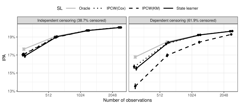
Figure 1: For the risk prediction models provided by each of the super learners, the IPA is plotted against sample size. The results are averages across 1000 simulated data sets and the error bars are used to quantify the Monte Carlo uncertainty.

We next compare the state learner to the super learner survSL [Westling et al., 2021]. This is another super learner which like the state learner works without a pre-specified censoring model. Note that both the state learner and survSL provide a prediction model for the event time outcome and also for the probability of being censored. Hence, we compare the performance of these methods with respect to both the outcome and the censoring distribution. Again we use the IPA to quantify the predictive performance.

The results are shown in Figures 2 and 3. We see that for most sample sizes, the state learner selected prediction models for both censoring and outcome which have similar or higher IPA compared to the prediction models selected by survSL.

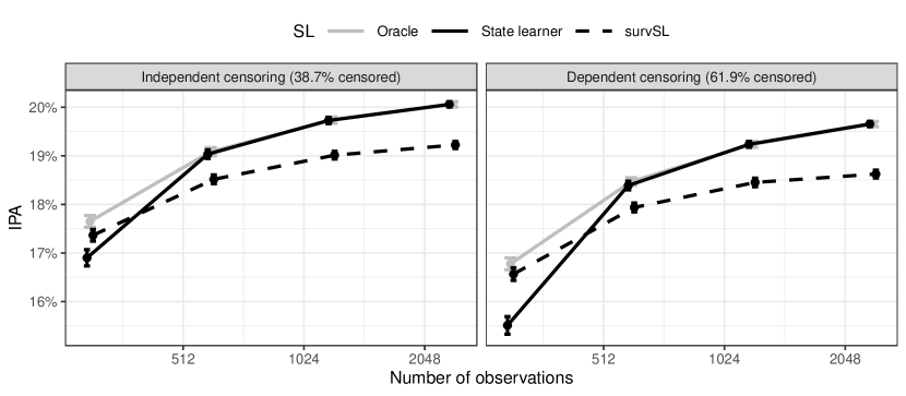
Figure 2: For the risk prediction models of the outcome provided by each of the super learners, the IPA at the fixed time horizon is plotted against sample size. The results are averages across 1000 repetitions and the error bars are used to quantify the Monte Carlo uncertainty.

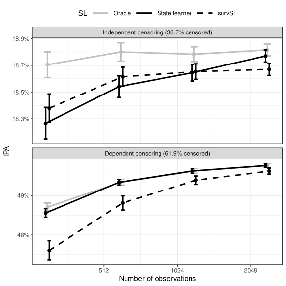
Figure 3: For the risk prediction models of the censoring model provided by each of the super learners, the IPA at the fixed time horizon is plotted against sample size. The results are averages across 1000 repetitions and the error bars are used to quantify the Monte Carlo uncertainty.

8 Prostate cancer study

In this section we use the prostate cancer data of Kattan et al. [2000] to illustrate the use of the state learner in the presence of competing risks. We have introduced the data in Section 7. The data consists of 1,042 patients who are followed from start of followup until tumor recurrence, death without tumor recurrence or end of followup (censored) whatever came first. For the sole purpose of illustration, we estimate the average treatment effect of hormone therapy on death and tumor recurrence. To do this we adapt the estimation strategy of Section 6 as follows. We use the state learner to rank libraries of learners for the cause-specific cumulative hazard functions of tumor recurrence, death without tumor recurrence, and censoring. The libraries of learners each include five learners: the Nelson-Aalen estimator, three Cox regression models (unpenalized, Lasso, Elastic net) each including additive effects of the 5 covariates (Section 7), and a random survival forest. We use the same set of learners to learn the cumulative hazard function of tumor recurrence $\Lambda_{1}$, the cumulative hazard function of death without tumor recurrence $\Lambda_{2}$, and the cumulative hazard function of the conditional censoring distribution $\Gamma$. We then use the highest ranked combination of learners and apply formula (16).

This gives a library consisting of $5^{3}=125$ learners for the conditional state occupation probability function $F$ defined in equation (5). We use five folds for training and testing the models, and we repeat training and evaluation five times with different splits. The integrated Brier score (defined in Section 4) for all learners are shown in Figure 4. We see that the prediction performance is mostly affected by the choice of learner for the censoring distribution. Several combinations of learners give similar performance as measured by the integrated Brier score, as long as a random forest is used to model the censoring distribution.

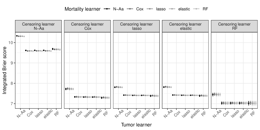
Figure 4: The results of applying the 125 combinations of learners to the prostate cancer data set. The error bars are based on five repetitions using different splits. We refer to learners of $\Lambda_{1}$, $\Lambda_{2}$, and $\Gamma$ as ‘Tumor learner’, ‘Mortality learner’, and ‘Censoring learner’, respectively.

We use the learners of the three cumulative hazard functions selected by the state learner and the estimator defined in Section 6.1, equation (16), to estimate the average treatment effect of hormone therapy on risk of tumor recurrence and death. The propensity score is estimated with a lasso model that includes all levels of interaction. The results are shown in Figure 5 for 6 month intervals after baseline with pointwise 95% confidence intervals. We see that hormone therapy decreases the risk of tumor recurrence and increases the risk of death without tumor recurrence, but that none of the estimated effects are statistically significant.

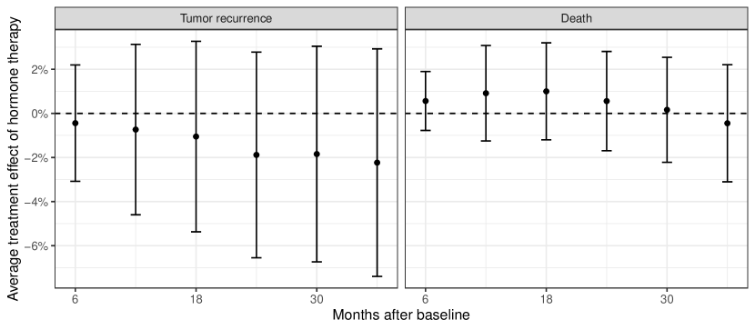
Figure 5: Estimates of the average treatment effect of hormone therapy on the risk of tumor recurrence and death obtained from the prostate cancer study analysed by Kattan et al. [2000]. The estimates are based on the estimator defined in equation (16) with pointwise 95% confidence intervals calculated as described in Section 6. The estimates of the nuisance parameters are provided by the state learner.

9 Discussion

The state learner is a new super learner that can be used with right-censored data and competing events. Compared to existing IPCW-based methods, the advantage of the state learner is that it does not depend on a pre-specified estimator of the censoring distribution, but selects one automatically based on a library of learners for the censoring distribution. Furthermore, the state learner neither requires that the cause-specific cumulative hazard functions $\Lambda_{j}$ can be written as integrals with respect to Lebesgue measure, nor does it assume a (semi-)parametric formula. In the remainder of this section we discuss the limitations of our proposal and avenues for further research.

A major advantage of the state learner is that the performance of each combination of learners can be estimated without additional nuisance parameters. A potential drawback of our approach is that we are evaluating the loss of the learners on the level of the observed data distribution while the target of the analysis is either the event time distribution, or the censoring distribution, or both. Specifically, the finite sample oracle inequality in Corollary 1 concerns the function $F$, which is a feature of $P\in\mathcal{P}$, while what we are typically interested in is $\Lambda_{j}$ or $S$, which are features of $Q\in\mathcal{Q}$. We emphasise that while the state learner provides us with estimates of $\Lambda_{j}$ and $\Gamma$ based on libraries $\mathcal{A}_{j}$ and $\mathcal{B}$, the performance of these learners is not assessed directly for their respective target parameters, but only indirectly via the performance of $F$. For settings without competing risks, our numerical studies suggest that measuring the performance of $F$ also leads to good performance for estimation of $S$.

Our proposed super learner can be implemented with a broad library of learners and using existing software. Furthermore, while the library $\mathcal{F}(\mathcal{A}_{1},\mathcal{A}_{2},\mathcal{B})$ consists of $|\mathcal{A}_{1}||\mathcal{A}_{2}||\mathcal{B}|$ many learners, we only need to fit $|\mathcal{A}_{1}|+|\mathcal{A}_{2}|+|\mathcal{B}|$ many learners in each fold. To evaluate the performance of each learner we need to perform $|\mathcal{A}_{1}||\mathcal{A}_{2}||\mathcal{B}|$ many operations to calculate the integrated Brier score in each hold-out sample, one for each combination of the fitted models, but these operations are often negligible compared to fitting the models. Hence the state learner is essentially not more computationally demanding than any procedure that uses super learning to learn $\Lambda_{1}$, $\Lambda_{2}$, and $\Gamma$ separately. While our proposal is based on constructing the library $\mathcal{F}$ from libraries for learning $\Lambda_{1}$, $\Lambda_{2}$, and $\Gamma$, it could also be of interest to consider learners that estimate $F$ directly.

In our numerical studies, we only considered learners of $\Lambda_{j}$ and $\Gamma$ that provide cumulative hazard functions which are piece-wise constant in the time argument. This simplifies the calculation of $F$ as the integrals in equation (6) reduce to sums. When $\Lambda_{j}$ or $\Gamma$ are absolutely continuous in the time argument, calculating $F$ is more involved, but we expect that a good approximation can be achieved by discretisation.

Appendix A Theoretical guarantees for the state learner

In this section we provide proofs of the results stated in Section 5.

Define $\bar{B}_{\tau,0}(F,o)=\bar{B}_{\tau}(F,o)-\bar{B}_{\tau}(F_{0},o)$ and $R_{0}(F)=P_{0}{[\bar{B}_{\tau,0}(F,\makebox[4.30554pt]{{$\cdot$}})]}$.

Lemma 1.

$R_{0}(F)=\|F-F_{0}\|_{P_{0}}^{2}$, where $\|\makebox[4.30554pt]{{$\cdot$}}\|_{P_{0}}$ is defined in equation (7).

Proof.

For any $t\in[0,\tau]$ and $j\in\{-1,0,1,2\}$ we have

$$\operatorname{\mathbb{E}}_{P_{0}}{\left[(F(t,j,X)-\mathds{1}{\{\eta(t)=j\}})^{2}\right]}$$

$$=\operatorname{\mathbb{E}}_{P_{0}}{\left[(F(t,j,X)-F_{0}(t,j,X)+F_{0}(t,j,X)-\mathds{1}{\{\eta(t)=j\}})^{2}\right]}$$

$$=\operatorname{\mathbb{E}}_{P_{0}}{\left[(F(t,j,X)-F_{0}(t,j,X))^{2}\right]}+\operatorname{\mathbb{E}}_{P_{0}}{\left[(F_{0}(t,j,X)-\mathds{1}{\{\eta(t)=j\}})^{2}\right]}$$

$$\quad+2\operatorname{\mathbb{E}}_{P_{0}}{\left[(F(t,j,X)-F_{0}(t,j,X))(F_{0}(t,j,X)-\mathds{1}{\{\eta(t)=j\}})\right]}$$

$$=\operatorname{\mathbb{E}}_{P_{0}}{\left[(F(t,j,X)-F_{0}(t,j,X))^{2}\right]}+\operatorname{\mathbb{E}}_{P_{0}}{\left[(F_{0}(t,j,X)-\mathds{1}{\{\eta(t)=j\}})^{2}\right]},$$

where the last equality follows from the tower property. Hence, using Fubini, we have

$$P{[\bar{B}_{\tau}(F,\makebox[4.30554pt]{{$\cdot$}})]}=\|F-F_{0}\|_{P_{0}}^{2}+P_{0}{[\bar{B}_{\tau}(F_{0},\makebox[4.30554pt]{{$\cdot$}})]}.$$

∎

Proof of Proposition 1.

The result follows from Lemma 1. ∎

Recall that $\mathcal{H}_{\mathcal{P}}$ denote the function space consisting of all conditional state occupation probability functions for some measure $P\in\mathcal{P}$.

Proof of Corollary 1.

First note that minimising the loss $\bar{B}_{\tau}$ is equivalent to minimising the loss $\bar{B}_{\tau,0}$, so the discrete super learner and oracle according to $\bar{B}_{\tau}$ and $\bar{B}_{\tau,0}$ are identical. By Lemma 1, $R_{0}(F)\geq 0$ for any $F\in\mathcal{H}_{\mathcal{P}}$, and so using Theorem 2.3 from [van der Vaart et al., 2006] with $p=1$, we have that for all $\delta>0$,

$$\operatorname{\mathbb{E}}_{P_{0}}{\left[R_{0}(\hat{\varphi}_{n}(\mathcal{D}_{n}^{-k}))\right]}$$

$$\quad\leq(1+2\delta)\operatorname{\mathbb{E}}_{P_{0}}{\left[R_{0}(\tilde{\varphi}_{n}(\mathcal{D}_{n}^{-k}))\right]}$$

$$\qquad+(1+\delta)\frac{16K}{n}\log(1+|\mathcal{F}_{n}|)\sup_{F\in\mathcal{H}_{\mathcal{P}}}\left\{M(F)+\frac{v(F)}{R_{0}(F)}\left(\frac{1}{\delta}+1\right)\right\}$$

where for each $F\in\mathcal{H}_{\mathcal{P}}$, $(M(F),v(F))$ is some Bernstein pair for the function $o\mapsto\bar{B}_{\tau,0}(F,o)$. As $\bar{B}_{\tau,0}(F,\makebox[4.30554pt]{{$\cdot$}})$ is uniformly bounded by $\tau$ for any $F\in\mathcal{H}_{\mathcal{P}}$, it follows from section 8.1 in [van der Vaart et al., 2006] that $(\tau,1.5P_{0}{[\bar{B}_{\tau,0}(F,\makebox[4.30554pt]{{$\cdot$}})^{2}]})$ is a Bernstein pair for $\bar{B}_{\tau,0}(F,\makebox[4.30554pt]{{$\cdot$}})$. Now, for any $a,b,c\in\mathbb{R}$ we have

$$(a-c)^{2}-(b-c)^{2} =(a-b+b-c)^{2}-(b-c)^{2}$$

$$=(a-b)^{2}+(b-c)^{2}+2(b-c)(a-b)-(b-c)^{2}$$

$$=(a-b)\left\{(a-b)+2(b-c)\right\}$$

$$=(a-b)\left\{a+b-2c\right\},$$

so using this with $a=F(t,j,x)$, $b=F_{0}(t,j,x)$, and $c=\mathds{1}{\{\eta(t)=j\}}$, we have by Jensen’s inequality

$$P_{0}{[\bar{B}_{\tau,0}(F,\makebox[4.30554pt]{{$\cdot$}})^{2}]}$$

$$\leq 2\tau\operatorname{\mathbb{E}}_{P_{0}}{\left[\sum_{j=-1}^{2}\int_{0}^{\tau}\left\{\left(F(t,j,X)-\mathds{1}{\{\eta(t)=j\}}\right)^{2}-\left(F_{0}(t,j,X)-\mathds{1}{\{\eta(t)=j\}}\right)^{2}\right\}^{2}\mathop{}\!\mathrm{d}t\right]}$$

$$=2\tau\operatorname{\mathbb{E}}_{P_{0}}\Bigg{[}\sum_{j=-1}^{2}\int_{0}^{\tau}\left(F(t,j,X)-F_{0}(t,j,X)\right)^{2}$$

$$\quad\quad\quad\quad\quad\quad\times\left\{F(t,j,X)+F_{0}(t,j,X)-2\mathds{1}{\{\eta(t)=j\}}\right\}^{2}\mathop{}\!\mathrm{d}t\Bigg{]}$$

$$\leq 8\tau\operatorname{\mathbb{E}}_{P_{0}}{\left[\sum_{j=-1}^{2}\int_{0}^{\tau}\left(F(t,j,X)-F_{0}(t,j,X)\right)^{2}\mathop{}\!\mathrm{d}t\right]}.$$

$$=8\tau\|F-F_{0}\|_{P_{0}}^{2}.$$

Thus when $v(F)=1.5P_{0}{[\bar{B}_{\tau,0}(F,\makebox[4.30554pt]{{$\cdot$}})^{2}]}$ we have by Lemma 1

$$\frac{v(F)}{R_{0}(F)}=1.5\frac{P_{0}{[\bar{B}_{\tau,0}(F,\makebox[4.30554pt]{{$\cdot$}})^{2}]}}{P_{0}{[\bar{B}_{\tau,0}(F,\makebox[4.30554pt]{{$\cdot$}})]}}\leq 12\tau,$$

and so using the Bernstein pairs $(\tau,1.5P_{0}{[\bar{B}_{\tau,0}(F,\makebox[4.30554pt]{{$\cdot$}})^{2}]})$ we have

$$\sup_{F\in\mathcal{H}_{\mathcal{P}}}\left\{M(F)+\frac{v(F)}{R_{0}(F)}\left(\frac{1}{\delta}+1\right)\right\}\leq\tau\left(13+\frac{12}{\delta}\right),$$

For all $\delta>0$ we thus have

$$\operatorname{\mathbb{E}}_{P_{0}}{\left[R_{0}(\hat{\varphi}_{n}(\mathcal{D}_{n}^{-k}))\right]}\leq (1+2\delta)\operatorname{\mathbb{E}}_{P_{0}}{\left[R_{0}(\tilde{\varphi}_{n}(\mathcal{D}_{n}^{-k}))\right]}$$

$$\quad+(1+\delta)\log(1+|\mathcal{F}_{n}|)\tau\frac{16K}{n}\left(13+\frac{12}{\delta}\right),$$

and then the final result follows from Lemma 1. ∎

Proof of Corollary 2.

By definition of the oracle and Lemma 1,

$$\operatorname{\mathbb{E}}_{P_{0}}{\left[\|\tilde{\varphi}_{n}(\mathcal{D}_{n}^{-k})-F_{0}\|_{P_{0}}^{2}\right]}\leq\operatorname{\mathbb{E}}_{P_{0}}{\left[\|\varphi_{n}(\mathcal{D}_{n}^{-k})-F_{0}\|_{P_{0}}^{2}\right]}$$

for all $n\in\mathbb{N}$. The results then follows from Corollary 1. ∎

Appendix B The state learner with targeted learning

In this section show that a product structure is preserved when an estimator $\bar{\Psi}(\hat{F}_{n},\hat{H}_{n})$ is used instead of $\tilde{\Psi}(\hat{\Lambda}_{n},\hat{\Gamma}_{n},\hat{H}_{n})$.

Proof of Proposition 2.

For notational convenience we suppress $X$ in the following. The final result can be obtained by adding the argument $X$ to all functions and averaging. We use the relations from equation (8) to write

$$\int_{0}^{\tau}w(s)\left\{\Gamma(s)-\hat{\Gamma}_{n}(s)\right\}[\Lambda-\hat{\Lambda}_{n}](\mathop{}\!\mathrm{d}s)$$

$$=\int_{0}^{\tau}w(s)\left\{\int_{0}^{s}\frac{F(\mathop{}\!\mathrm{d}u,2)}{F(u-,0)}-\int_{0}^{s}\frac{\hat{F}_{n}(\mathop{}\!\mathrm{d}u,2)}{\hat{F}_{n}(u-,0)}-\right\}\left[\frac{F(\mathop{}\!\mathrm{d}s,1)}{F(s-,0)}-\frac{\hat{F}_{n}(\mathop{}\!\mathrm{d}s,1)}{\hat{F}_{n}(s-,0)}\right]$$

$$=\int_{0}^{\tau}w(s)\Bigg{\{}\int_{0}^{s}\left(\frac{1}{F(u-,0)}-\frac{1}{\hat{F}_{n}(u-,0)}\right)F(\mathop{}\!\mathrm{d}u,2)$$

$$\qquad\qquad\qquad+\int_{0}^{s}\frac{1}{\hat{F}_{n}(u-,0)}\left[F(\mathop{}\!\mathrm{d}u,2)-\hat{F}_{n}(\mathop{}\!\mathrm{d}u,2)\right]\Bigg{\}}$$

$$\qquad\qquad\times\left[\left(\frac{1}{F(s-,0)}-\frac{1}{\hat{F}_{n}(s-,0)}\right)F(\mathop{}\!\mathrm{d}s,1)+\frac{1}{\hat{F}_{n}(s-,0)}\left(F(\mathop{}\!\mathrm{d}s,1)-\hat{F}_{n}(\mathop{}\!\mathrm{d}s,1)\right)\right]$$

$$=\int_{0}^{\tau}\int_{0}^{s}w(s)\left(\frac{1}{F(u-,0)}-\frac{1}{\hat{F}_{n}(u-,0)}\right)\left(\frac{1}{F(s-,0)}-\frac{1}{\hat{F}_{n}(s-,0)}\right)F(\mathop{}\!\mathrm{d}u,2)F(\mathop{}\!\mathrm{d}s,1)$$

$$\quad+\int_{0}^{\tau}\int_{0}^{s}w(s)\left(\frac{1}{F(u-,0)}-\frac{1}{\hat{F}_{n}(u-,0)}\right)\frac{F(\mathop{}\!\mathrm{d}u,2)}{\hat{F}_{n}(u-,0)}\left(F(\mathop{}\!\mathrm{d}s,1)-\hat{F}_{n}(\mathop{}\!\mathrm{d}s,1)\right)$$

$$\quad+\int_{0}^{\tau}\int_{0}^{s}\frac{w(s)}{\hat{F}_{n}(u-,0)}\left[F(\mathop{}\!\mathrm{d}u,2)-\hat{F}_{n}(\mathop{}\!\mathrm{d}u,2)\right]\left(\frac{1}{F(s-,0)}-\frac{1}{\hat{F}_{n}(s-,0)}\right)F(\mathop{}\!\mathrm{d}s,1)$$

$$\quad+\int_{0}^{\tau}\int_{0}^{s}\frac{w(s)}{\hat{F}_{n}(u-,0)}\left[F(\mathop{}\!\mathrm{d}u,2)-\hat{F}_{n}(\mathop{}\!\mathrm{d}u,2)\right]\frac{1}{\hat{F}_{n}(s-,0)}\left(F(\mathop{}\!\mathrm{d}s,1)-\hat{F}_{n}(\mathop{}\!\mathrm{d}s,1)\right).$$

Consider the first term on the right hand side. Defining

$$w_{n}^{*}(t)=\left(F(t-,0)-\hat{F}_{n}(t-,0)\right)\left(\frac{1}{F(t-,0)}-\frac{1}{\hat{F}_{n}(t-,0)}\right),$$

we can write

$$\int_{0}^{\tau}\int_{0}^{s}w(s)\left(\frac{1}{F(u-,0)}-\frac{1}{\hat{F}_{n}(u-,0)}\right)\left(\frac{1}{F(s-,0)}-\frac{1}{\hat{F}_{n}(s-,0)}\right)F(\mathop{}\!\mathrm{d}u,2)F(\mathop{}\!\mathrm{d}s,1)$$

$$=\int_{0}^{\tau}\int_{0}^{s}w(s)w_{n}^{*}(u)\left(F(u-,0)-\hat{F}_{n}(u-,0)\right)$$

$$\qquad\qquad\quad\times w_{n}^{*}(s)\left(F(s-,0)-\hat{F}_{n}(s-,0)\right)F(\mathop{}\!\mathrm{d}u,2)F(\mathop{}\!\mathrm{d}s,1)$$

$$=\int_{0}^{\tau}\int_{0}^{s}w_{n}^{a}(s,u)\left(F(u-,0)-\hat{F}_{n}(u-,0)\right)\left(F(s-,0)-\hat{F}_{n}(s-,0)\right)F(\mathop{}\!\mathrm{d}u,2)F(\mathop{}\!\mathrm{d}s,1),$$

where we have defined $w_{n}^{a}(s,u)=w(s)w^{*}_{n}(s)w^{*}_{n}(u)$. By assumption, $w_{n}^{a}(s,u)$ is uniformly bounded. The same approach can be applied to the three remaining terms which gives the result. ∎

References

• Andersen et al. [2003] P. K. Andersen, J. P. Klein, and S. Rosthøj. Generalised linear models for correlated pseudo-observations, with applications to multi-state models. Biometrika, 2003.
• Andersen et al. [2012] P. K. Andersen, O. Borgan, R. D. Gill, and N. Keiding. Statistical models based on counting processes. Springer Science & Business Media, 2012.
• Begun et al. [1983] J. M. Begun, W. J. Hall, W.-M. Huang, and J. A. Wellner. Information and asymptotic efficiency in parametric-nonparametric models. The Annals of Statistics, 11(2):432–452, 1983.
• Benichou and Gail [1990] J. Benichou and M. H. Gail. Estimates of absolute cause-specific risk in cohort studies. Biometrics, pages 813–826, 1990.
• Bickel et al. [1993] P. J. Bickel, C. A. Klaassen, Y. Ritov, and J. A. Wellner. Efficient and adaptive estimation for semiparametric models, volume 4. Johns Hopkins University Press Baltimore, 1993.
• Breiman [1996] L. Breiman. Stacked regressions. Machine learning, 24(1):49–64, 1996.
• Brier et al. [1950] G. W. Brier et al. Verification of forecasts expressed in terms of probability. Monthly weather review, 78(1):1–3, 1950.
• Chernozhukov et al. [2018] V. Chernozhukov, D. Chetverikov, M. Demirer, E. Duflo, C. Hansen, W. Newey, and J. Robins. Double/debiased machine learning for treatment and structural parameters, 2018.
• Cox [1972] D. R. Cox. Regression models and life-tables. Journal of the Royal Statistical Society: Series B (Methodological), 34(2):187–202, 1972.
• Fan and Gijbels [1996] J. Fan and I. Gijbels. Local polynomial modelling and its applications. Routledge, 1996.
• Fisher and Kennedy [2021] A. Fisher and E. H. Kennedy. Visually communicating and teaching intuition for influence functions. The American Statistician, 75(2):162–172, 2021.
• Gensheimer and Narasimhan [2019] M. F. Gensheimer and B. Narasimhan. A scalable discrete-time survival model for neural networks. PeerJ, 7:e6257, 2019.
• Gerds [2019] T. A. Gerds. prodlim: Product-Limit Estimation for Censored Event History Analysis, 2019. URL https://CRAN.R-project.org/package=prodlim. R package version 2019.11.13.
• Gerds and Kattan [2021] T. A. Gerds and M. W. Kattan. Medical risk prediction models: with ties to machine learning. CRC Press, 2021.
• Gerds and Schumacher [2006] T. A. Gerds and M. Schumacher. Consistent estimation of the expected Brier score in general survival models with right-censored event times. Biometrical Journal, 48(6):1029–1040, 2006.
• Gerds et al. [2013] T. A. Gerds, M. W. Kattan, M. Schumacher, and C. Yu. Estimating a time-dependent concordance index for survival prediction models with covariate dependent censoring. Statistics in medicine, 32(13):2173–2184, 2013.
• Gerds et al. [2023] T. A. Gerds, J. S. Ohlendorff, and B. Ozenne. riskRegression: Risk Regression Models and Prediction Scores for Survival Analysis with Competing Risks, 2023. URL https://CRAN.R-project.org/package=riskRegression. R package version 2023.03.22.
• Gill et al. [1997] R. D. Gill, M. J. van der Laan, and J. M. Robins. Coarsening at random: Characterizations, conjectures, counter-examples. In Proceedings of the First Seattle Symposium in Biostatistics, pages 255–294. Springer, 1997.
• Gneiting and Raftery [2007] T. Gneiting and A. E. Raftery. Strictly proper scoring rules, prediction, and estimation. Journal of the American statistical Association, 102(477):359–378, 2007.
• Golmakani and Polley [2020] M. K. Golmakani and E. C. Polley. Super learner for survival data prediction. The International Journal of Biostatistics, 16(2):20190065, 2020.
• Gonzalez Ginestet et al. [2021] P. Gonzalez Ginestet, A. Kotalik, D. M. Vock, J. Wolfson, and E. E. Gabriel. Stacked inverse probability of censoring weighted bagging: A case study in the infcarehiv register. Journal of the Royal Statistical Society Series C: Applied Statistics, 70(1):51–65, 2021.
• Graf et al. [1999] E. Graf, C. Schmoor, W. Sauerbrei, and M. Schumacher. Assessment and comparison of prognostic classification schemes for survival data. Statistics in medicine, 1999.
• Han et al. [2021] X. Han, M. Goldstein, A. Puli, T. Wies, A. Perotte, and R. Ranganath. Inverse-weighted survival games. Advances in Neural Information Processing Systems, 34, 2021.
• Hernán and Robins [2020] M. Hernán and J. Robins. Causal Inference: What If. Boca Raton: Chapman & Hall/CRC, 2020.
• Hines et al. [2022] O. Hines, O. Dukes, K. Diaz-Ordaz, and S. Vansteelandt. Demystifying statistical learning based on efficient influence functions. The American Statistician, 76(3):292–304, 2022.
• Hothorn et al. [2006] T. Hothorn, P. Bühlmann, S. Dudoit, A. Molinaro, and M. J. van der Laan. Survival ensembles. Biostatistics, 7(3):355–373, 2006.
• Ishwaran and Kogalur [2023] H. Ishwaran and U. Kogalur. Fast Unified Random Forests for Survival, Regression, and Classification (RF-SRC), 2023. URL https://cran.r-project.org/package=randomForestSRC. R package version 3.2.2.
• Ishwaran et al. [2008] H. Ishwaran, U. B. Kogalur, E. H. Blackstone, and M. S. Lauer. Random survival forests. The annals of applied statistics, 2(3):841–860, 2008.
• Jewell et al. [2007] N. P. Jewell, X. Lei, A. C. Ghani, C. A. Donnelly, G. M. Leung, L.-M. Ho, B. J. Cowling, and A. J. Hedley. Non-parametric estimation of the case fatality ratio with competing risks data: an application to severe acute respiratory syndrome (sars). Statistics in medicine, 26(9):1982–1998, 2007.
• Kaplan and Meier [1958] E. L. Kaplan and P. Meier. Nonparametric estimation from incomplete observations. Journal of the American statistical association, 53(282):457–481, 1958.
• Kattan and Gerds [2018] M. W. Kattan and T. A. Gerds. The index of prediction accuracy: an intuitive measure useful for evaluating risk prediction models. Diagnostic and prognostic research, 2018.
• Kattan et al. [2000] M. W. Kattan, M. J. Zelefsky, P. A. Kupelian, P. T. Scardino, Z. Fuks, and S. A. Leibel. Pretreatment nomogram for predicting the outcome of three-dimensional conformal radiotherapy in prostate cancer. Journal of clinical oncology, 18(19):3352–3359, 2000.
• Katzman et al. [2018] J. L. Katzman, U. Shaham, A. Cloninger, J. Bates, T. Jiang, and Y. Kluger. Deepsurv: personalized treatment recommender system using a Cox proportional hazards deep neural network. BMC medical research methodology, 18(1):1–12, 2018.
• Keles et al. [2004] S. Keles, M. van der Laan, and S. Dudoit. Asymptotically optimal model selection method with right censored outcomes. Bernoulli, 10(6):1011–1037, 2004.
• Kennedy [2016] E. H. Kennedy. Semiparametric theory and empirical processes in causal inference. In Statistical causal inferences and their applications in public health research, pages 141–167. Springer, 2016.
• Kennedy [2022] E. H. Kennedy. Semiparametric doubly robust targeted double machine learning: a review. arXiv preprint arXiv:2203.06469, 2022.
• Kvamme and Borgan [2021] H. Kvamme and Ø. Borgan. Continuous and discrete-time survival prediction with neural networks. Lifetime Data Analysis, 27(4):710–736, 2021.
• Lee et al. [2018] C. Lee, W. Zame, J. Yoon, and M. van der Schaar. Deephit: A deep learning approach to survival analysis with competing risks. In Proceedings of the AAAI conference on artificial intelligence, volume 32, 2018.
• Lee et al. [2021] D. K. Lee, N. Chen, and H. Ishwaran. Boosted nonparametric hazards with time-dependent covariates. Annals of Statistics, 49(4):2101, 2021.
• Li et al. [2016] Y. Li, K. S. Xu, and C. K. Reddy. Regularized parametric regression for high-dimensional survival analysis. In Proceedings of the 2016 SIAM International Conference on Data Mining, pages 765–773. SIAM, 2016.
• Mogensen and Gerds [2013] U. B. Mogensen and T. A. Gerds. A random forest approach for competing risks based on pseudo-values. Statistics in medicine, 32(18):3102–3114, 2013.
• Molinaro et al. [2004] A. M. Molinaro, S. Dudoit, and M. J. van der Laan. Tree-based multivariate regression and density estimation with right-censored data. Journal of Multivariate Analysis, 90(1):154–177, 2004.
• Ozenne et al. [2017] B. Ozenne, A. L. Sørensen, T. Scheike, C. Torp-Pedersen, and T. A. Gerds. riskregression: Predicting the risk of an event using Cox regression models. R Journal, 9(2):440–460, 2017.
• Pfanzagl and Wefelmeyer [1982] J. Pfanzagl and W. Wefelmeyer. Contributions to a general asymptotic statistical theory. Springer, 1982.
• Polley et al. [2023] E. Polley, E. LeDell, C. Kennedy, and M. van der Laan. SuperLearner: Super Learner Prediction, 2023. URL https://CRAN.R-project.org/package=SuperLearner. R package version 2.0-28.1.
• Rytgaard and van der Laan [2022] H. C. Rytgaard and M. J. van der Laan. Targeted maximum likelihood estimation for causal inference in survival and competing risks analysis. Lifetime Data Analysis, pages 1–30, 2022.
• Rytgaard et al. [2021] H. C. Rytgaard, F. Eriksson, and M. J. van der Laan. Estimation of time-specific intervention effects on continuously distributed time-to-event outcomes by targeted maximum likelihood estimation. Biometrics, 2021.
• Sachs et al. [2019] M. C. Sachs, A. Discacciati, Å. H. Everhov, O. Olén, and E. E. Gabriel. Ensemble prediction of time-to-event outcomes with competing risks: A case-study of surgical complications in Crohn’s disease. Journal of the Royal Statistical Society Series C: Applied Statistics, 68(5):1431–1446, 2019.
• Steingrimsson et al. [2019] J. A. Steingrimsson, L. Diao, and R. L. Strawderman. Censoring unbiased regression trees and ensembles. Journal of the American Statistical Association, 2019.
• Therneau [2022] T. M. Therneau. A Package for Survival Analysis in R, 2022. URL https://CRAN.R-project.org/package=survival. R package version 3.4-0.
• Tsiatis [2007] A. Tsiatis. Semiparametric theory and missing data. Springer Science & Business Media, 2007.
• van der Laan and Dudoit [2003] M. J. van der Laan and S. Dudoit. Unified cross-validation methodology for selection among estimators and a general cross-validated adaptive epsilon-net estimator: Finite sample oracle inequalities and examples. Technical report, Division of Biostatistics, University of California, 2003.
• van der Laan and Robins [2003] M. J. van der Laan and J. M. Robins. Unified methods for censored longitudinal data and causality. Springer Science & Business Media, 2003.
• van der Laan and Rose [2011] M. J. van der Laan and S. Rose. Targeted learning: causal inference for observational and experimental data. Springer Science & Business Media, 2011.
• van der Laan et al. [2007] M. J. van der Laan, E. C. Polley, and A. E. Hubbard. Super learner. Statistical applications in genetics and molecular biology, 6(1), 2007.
• van der Vaart [2000] A. W. van der Vaart. Asymptotic statistics, volume 3. Cambridge university press, 2000.
• van der Vaart et al. [2006] A. W. van der Vaart, S. Dudoit, and M. J. van der Laan. Oracle inequalities for multi-fold cross validation. Statistics & Decisions, 24(3):351–371, 2006.
• Verweij and van Houwelingen [1993] P. J. Verweij and H. C. van Houwelingen. Cross-validation in survival analysis. Statistics in medicine, 12(24):2305–2314, 1993.
• Westling et al. [2021] T. Westling, A. Luedtke, P. Gilbert, and M. Carone. Inference for treatment-specific survival curves using machine learning. arXiv preprint arXiv:2106.06602, 2021.
• Wolpert [1992] D. H. Wolpert. Stacked generalization. Neural networks, 5(2):241–259, 1992.
• Yao et al. [2017] J. Yao, X. Zhu, F. Zhu, and J. Huang. Deep correlational learning for survival prediction from multi-modality data. In International conference on medical image computing and computer-assisted intervention, pages 406–414. Springer, 2017.