Surface reconstruction of sampled textiles via Morse theory

Abstract

In this work, we study the perception problem for garments using tools from computational topology: the identification of their geometry and position in space from point-cloud samples, as obtained e.g. with 3D scanners. We present a reconstruction algorithm based on a direct topological study of the sampled textile surface that allows us to obtain a cellular decomposition of it via a Morse function. No intermediate triangulation or local implicit equations are used, avoiding reconstruction-induced artifices. No a priori knowledge of the surface topology, density or regularity of the point-sample is required to run the algorithm. The results are a piecewise decomposition of the surface as a union of Morse cells (i.e. topological disks), suitable for tasks such as noise-filtering or mesh-independent reparametrization, and a cell complex of small rank determining the surface topology. This algorithm can be applied to smooth surfaces with or without boundary, embedded in an ambient space of any dimension.

1 Introduction

Robotic manipulation of cloth in a domestic environment is an increasingly relevant problem because of the ubiquitous presence of textiles in human activities; with promising applications ranging from automated folding to dressing disabled people [[Doumanoglou2016, Garcia-Camacho2020]]. When an arbitrary and unknown garment is presented before the robot, a point-sample of it can be obtained through the use of depth-cameras or 3D-scanners. Nevertheless, these points will in general have no known structure. This is where reconstructing and recognizing the textile from the point-cloud (i.e. to parametrize and deduce its topology) becomes of great importance if one wishes the robot to manipulate the garment [[yin2021modeling]].

Arguably, the main challenge faced in the automated manipulation of cloth is the high number of deformation states that textiles can present [[Corrales2018]]. In contrast to rigid body manipulation, where the dynamics of the manipulated object are very well understood [[Taylor:2005:CM]], there is not one single physical model that can be considered best in terms of describing the dynamics of real textiles [[Nealen:2006:PDM]]. In any case, physical models of cloth behavior remain useful for developing planning and control strategies [[Li2015, Colome2018]]; as well as for generating the massive data required to train learning algorithms before their deployment and tuning in the real world [[jangir2020dynamic, Colome2020]]. For all of these tasks it is crucial to have an accurate and fast-to-compute reconstruction of the garment to be controlled/simulated.

Naturally, because of the previous reasons, the reconstruction of a surface in space from a sample of points on it is a question to which considerable attention has been devoted in the areas of Computational Geometry and Computer Graphics (see [[Dey2006CurveAS]] for algorithms with mathematical guarantees and [[huang2022surface]] for a survey of state-of-the-art methods). Common algorithms involve triangulating the cloud points, fitting local implicit functions or more recently applying learning (i.e. Neural Networks) methods. Nevertheless, to our knowledge almost all these algorithms disregard a direct topological study of the point-cloud. Moreover, most of them focus on reconstructing watertight surfaces (i.e. without boundary). Applying this kind of algorithms to point-clouds coming from garments can lead to incorrect results since textiles can be naturally realized as surfaces with boundary, which is coincidentally what the majority of physical models assume in order to simulate them. One of the reasons for this focus on reconstructing surfaces without boundary may be the challenge associated in detecting boundaries of point-cloud surfaces (see [[MINEO201981]]): the problem is in general ill-posed since regions of the cloud with low density could be mistaken for boundaries of the underlying surface (e.g. think about removing small disks in a point-cloud coming from a sphere).

In this work, we present a novel reconstruction algorithm that proceeds directly from a point-cloud to obtain a cellular decomposition of the cloth surface: a global piecewise decomposition of the surface is found, with a small number of pieces which are parametrized disks. No intermediate triangulation or local implicit equations are used, avoiding reconstruction-induced artifices. The algorithm is robust: it always produces a surface, and it captures the topological features of the sampled surface with a size greater than the average distance between sample points. From the cellular decomposition, the topology of the surface can be deduced immediately. To obtain this decomposition, we present for the first time in literature (to our knowledge) an algorithm to determine how (discrete) Morse cells attach to each order (see Figure 1). Furthermore, for the case of surfaces with boundary, we develop a novel graph-theoretical method to determine robustly boundary points of the cloud.

Our decomposition algorithm was first sketched by the authors in two proceedings papers [[MorseEACA, MorseCEIG2]]. Here we expand greatly on that work to give full explanations on how to treat the case of surfaces with boundary, we explain for the first time in detail the theory behind our method, we give a full algorithm on how to compute the Morse cells and their attachment maps, we discuss and present results on the problem of how to parameterize the cell decomposition by flat patches and we reconstruct novel challenging point-clouds of surfaces with boundary.

1.1 Organization

The remainder of this paper is organized as follows: in Section 2 we review literature from computational and differential topology related to our method; then in Section 3 we explain and develop the theoretical machinery –coming from smooth Morse theory– needed to apply our algorithm successfully. In Section 4 we initiate the study of the point-cloud, giving it local structure by finding neighbors for each point, their tangent planes and the boundary curves. Section LABEL:sec_morse_celdas deals with the computation of the Morse flow, critical points, Morse cells and how they attach to each other, and it is one of the main contributions of this work. Finally, in Section LABEL:sec:param2cells we explain how to parametrize the $2$-cells by flat regions of the plane; and in Section LABEL:sec_results we present the reconstruction of five challenging point-clouds (four with boundary, one of them being a real 3D scan of a garment) using the presented algorithm.

2 Related work

Since its beginnings, Differential Topology has tackled the piecewise parametrization problem for manifolds through Morse functions. A smooth map $f:M\to\mathbb{R}$ defined on a compact manifold without boundary is Morse if it has only finitely many critical points, and at all of these the Hessian $H(f)$ is nondegenerate. Classical Morse theory (see [[Hirsch1976DiffTopo]]) shows that a generic Morse function $f$ induces, through its gradient flow, two decompositions of the manifold $M$:

1. As a CW complex (see [[Munkres1984ElementsOA]]): Each critical point of $f$, together with its unstable manifold for the vector field $-\nabla f$, forms a cell which is topologically a ball, whose boundary attaches to lower-dimensional cells (see Figure 1). A global piecewise parametrization of $M$ is achieved, and a Morse-Smale complex, with the critical points of $f$ as a basis, giving the singular homology of $M$.

2. As level sets: $M$ is foliated by the level sets $f^{-1}(c)$. For regular values $c$ these level sets are submanifolds of $M$ with codimension 1, with a diffeomorphism $f^{-1}(c_{1})\cong f^{-1}(c_{2})$ if no critical value of $f$ lies between $c_{1}$ and $c_{2}$. The transformation of the level set when $c$ crosses a critical value of $f$ is a surgery (see [[Hirsch1976DiffTopo]] and Section 3).

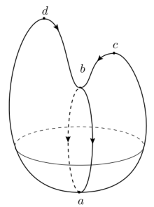
Figure 1: Critical points of the Morse-Smale function $f(x,y,z)=z$ on an example surface. The cellular decomposition is obtained by gluing two $2$-cells each containing $d$ and $c$ (the maxima) along the curve through $b$ (the saddle point) and $a$ (the minimum).

The success of Morse theory comes from the fact that Morse functions, and the Morse-Smale transversality conditions required for the above analysis, are generic among $\mathcal{C}^{2}$ maps from $M$ to $\mathbb{R}$. For instance, the height function in a random direction in $\mathbb{R}^{N}$ has probability 1 of being a Morse-Smale function, i.e. the measure of the set where the height function is not Morse-Smale is zero. Morse theory also extends to manifolds with boundary via stratified spaces [[Goresky1988StratifiedMT]] as we explain in detail in this work.

Applying Morse theoretical ideas directly to the sample point-cloud of a surface $S$ was first suggested by [[Gao2008MorseSmaleD, Zhu2009TopologicalDP]], who propose an algorithm for point-clouds with a known, homogeneous density of sampling. Later, in [[Cazals2013TowardsMT]] a Morse decomposition scheme from point-clouds sampling manifolds without boundary of any dimension is proposed. All these works, however, stop short of questions such as cell parametrization or attachment maps, which are relevant to robotic applications where point-clouds of textiles may need to be filtered and down-sampled in order to be simulated or controlled as explained in the introduction. We use the gradient flows of [[Gao2008MorseSmaleD, Zhu2009TopologicalDP]] as the starting point, but then detect critical points and their Morse cells differently, proposing a new procedure based on studying the level sections of these flows.

3 Preliminaries: smooth Morse theory

In this section we present a summary of smooth Morse theory for surfaces with and without boundary. We first explain briefly the case without boundary, which encapsulates the main ideas of the field. For a summary of this part, including what is needed to run our algorithm see Section 3.3.

3.1 Morse theory for surfaces without boundary

Let $S\subset\mathbb{R}^{N}$ be a smooth compact surface without boundary. The goal is to decompose any given $S$ as in Figure 1. In order to do that, we will compute its Morse-Smale complex, which in the case of a surface only consists of $0$-cells (points), $1$-cells (curves) and $2$-cells (topological disks).

As explained before, a map $f:S\to\mathbb{R}$ is Morse if it is $\mathcal{C}^{2}$, has only finitely many critical points (i.e. points $p$ where $\text{d}_{p}f=\nabla f(p)=0$), and at all of these its Hessian has rank $2$.

Definition 1 (Morse data).

For each critical point $p\in S$, the Morse data are the pair of sets $\left(A(p),B(p)\right)$ where

$$A(p):=\mathcal{B}(p)\cap f^{-1}\left([f(p)-\epsilon,f(p)+\epsilon]\right),$$

with $\mathcal{B}(p)\subset\mathbb{R}^{N}$ a closed ball around $p$ of sufficiently small radius, the value of $\epsilon>0$ is such that there are not more critical points of $f$ in $f^{-1}\left([f(p)-\epsilon,f(p)+\epsilon]\right)$ and $B(p):=\mathcal{B}(p)\cap f^{-1}\left(f(p)-\epsilon\right)$. Notice that $B(p)\subseteq\partial A(p)$. See Figure 2 for examples of the sets $A,B$.

Theorem 1 (Main theorem of Morse theory).

Let us now denote $f_{\leq c}=f^{-1}\left((-\infty,c]\right),f_{c}=f^{-1}(c)$. Then (see [[Hirsch1976DiffTopo]]) as $c\in\mathbb{R}$ increases only two things can happen:

A

If $c_{1}<c_{2}$ and there are no critical values of $f$ between them, then $f_{\leq c_{1}}$ and $f_{\leq c_{2}}$ have the same topology (they are actually diffeomorphic).

B

If there is a single critical point $p\in S$ such that $c_{1}<f(p)<c_{2}$ then $f_{\leq c_{2}}$ is obtained, up to diffeomorphism, from $f_{\leq c_{1}}$ by attaching the cell $A(p)$ along $B(p)$, i.e. $f_{\leq c_{2}}\simeq\left(f_{\leq c_{1}}\cup A(p)\right)/\sim$ where the equivalence relation is given by identifying $B(p)\subseteq f_{\leq c_{1}}$ with points of $\partial A(p)\supseteq B(p)$.

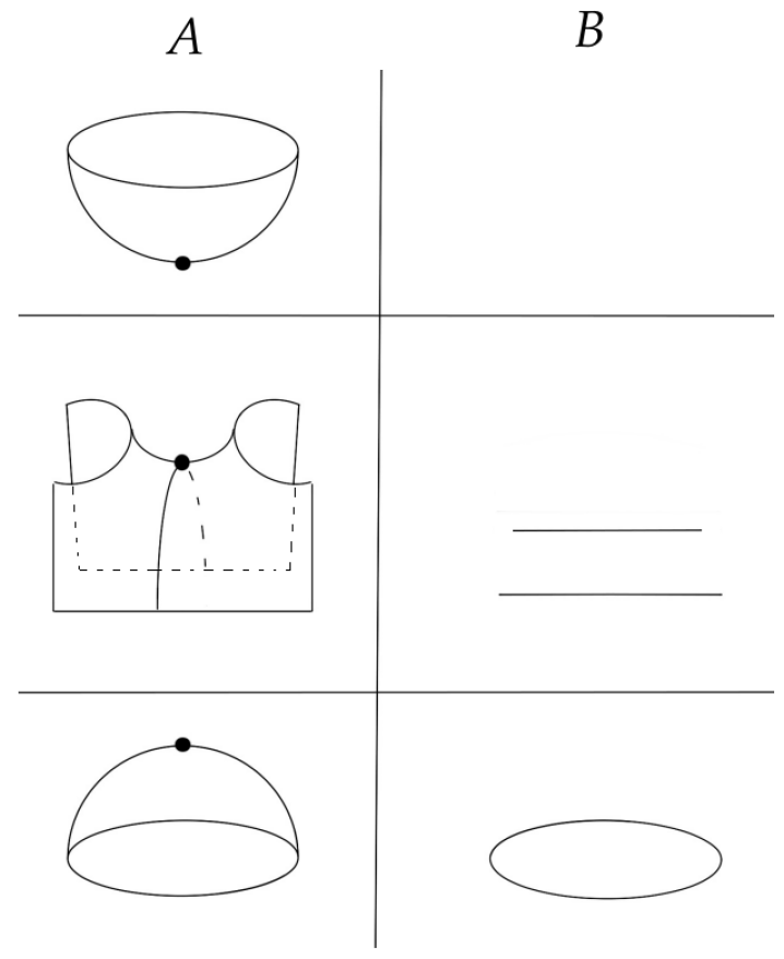
Figure 2: Three types of critical points $p$ (from top to bottom: minima, saddles and maxima) and their Morse data $(A(p),B(p))$ for surfaces without boundary.

The previous theorem is useful because it allows us to deduce how to couple each type of critical point with the Morse cells that will give us the sought decomposition of the surface under study (e.g. Figure 1). Since $H(f)$ has rank 2 at $p$, we can only have three types of critical points (see Figure 2) according to their index (number of negative eigenvalues of $H(f)$):

1. Minima: $A(p)$ is homeomorphic to a disk and $B(p)=\emptyset$. In this case there is no surgery, the cell $A(p)$ just appears. This cell retracts to a point, the local minimum, which will be a $0$-cell in the Morse-Smale complex.

2. Saddles: $A(p)$ is a quadrilateral (homeomorphic to a disk) and $B(p)$ consists of two segments. Two opposite sides of $\partial A(p)$ are identified with $B(p)$ (see Figure 2). The attachment of the cell $A(p)$ along $B(p)$ is homotopy-equivalent to the attachment of a $1$-cell, namely the medial axis of $A(p)$ to the middle points of $B(p)$.

3. Maxima: $A(p)=D$ is homeomorhic to a disk and $B(p)=\partial D$ is its boundary. The attachment map identifies $\partial A(p)$ with $B(p)$. This surgery adds a $2$-cell to the complex.

In summary, minima generate $0$-cells of the complex, saddle points $1$-cells and maxima $2$-cells. For instance, in Figure 1 there is one $0$-cell (point $a$), one $1$-cell (the closed curve passing trough $a$ and $b$) and two $2$-cells (one containing $d$ and the other $c$).

3.2 Morse theory for surfaces with boundary

Morse theory also extends to manifolds with boundary via stratified spaces [[Goresky1988StratifiedMT]]. Since stratified Morse theory is less well known and in [[Goresky1988StratifiedMT]] no explicit construction is given for manifolds with boundary, in this short section and in the appendix we give more details on how the boundaries affect the cellular decomposition and the transition between level sets using the terminology presented in the previous section for the case without boundary.

Definition 2 (Morse function).

We say that a $\mathcal{C}^{2}$ map $f:M\to\mathbb{R}$ defined in a manifold $M$ with boundary $\partial M$ is Morse if

1. it is Morse in the interior of $M$,

2. its restriction to $\partial M$, $g:=f_{|\partial M}$ is also a Morse function,

3. if $p\in\partial M$ is a critical point of $g$ then $\ker(\text{d}_{p}f)=\{0\}$.

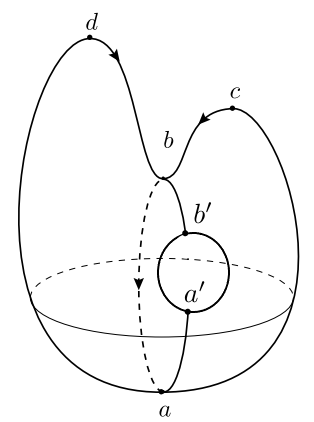
Figure 3: Critical points of the Morse-Smale function $f(x,y,z)=z$ on an example surface with boundary. Notice that now we have a boundary maximum $b^{\prime}$ and a boundary minimum $a^{\prime}$ since we have removed a disk.

As in the previous section we will focus in the case $M=S$ is a surface. Notice that now we can have critical points of $f_{|\partial S}$ in the boundary curves $\partial S$ that are not critical points of $f$ in the whole of $S$. Those are only 2 new cases which we call boundary minima and maxima (since $\partial S$ is a curve, there can not be saddle points of $g$, see Figure 3). These critical points will be responsible for generating new Morse cells depending on whether they are also local maxima or minima of the full surface or not (see Section 3.3). On a technical side, the third condition of the previous definition rules out the possibility that critical points located at $\partial S$ are saddle points of $f$ in $S$.

3.3 Construction of the Morse-Smale complex

We now make a summary of the effect of each critical point on the cell complex once we have made the appropriate deformation retracts. Recall that $0$-cells are points, $1$-cells are curves and $2$-cells are topological disks. Boundary curves of $\partial S$ will be part of the complex as $1$-cells.

1. Interior maximum: attach a $2$-cell to the $1$-cells as before.

2. Interior saddle: attach a $1$-cell to the $0$-cells as before or to a point of the boundary (this point becomes a new $0$-cell).

3. Interior minimum: add a $0$-cell to the skeleton as before.

4. Local maximum of $S$ located in $\partial S$: attach a $1$-cell to a $0$-cell (on the boundary) and attach a $2$-cell to the $1$-cells.

5. Boundary maximum (not of $S$): attach a $1$-cell to a $0$-cell (on the boundary).

6. Local minimum of $S$ located in $\partial S$: add a $0$-cell to the skeleton (this point will be on the boundary).

7. Boundary minimum (not of $S$): add a $0$-cell (boundary point) to the skeleton and attach a $1$-cell to a $0$-cell or to a point of the boundary (this point becomes a new $0$-cell).

In order to construct the complex, we first add all the $0$-cells (all interior, boundary minima and possibly some points of the boundary), then the $1$-cells (the boundary curves, the $1$-cells corresponding to each saddle point and the $1$-cells joining boundary minima to local minima or boundary points) and finally add the $2$-cells corresponding to each local maximum.

Remark 1.

A delicate point that we have not discussed yet, but will be crucial for our algorithm, is how to compute which cells attach to which cells (these are called the attachment maps). This problem will be addressed in detail for point-clouds in Section LABEL:sec_morse_celdas.

4 Structure of the point-cloud

Before we can define the flow of a Morse function on a given point-cloud $X$, we will need to give it a local structure. This is done by finding local neighbors to each point, which allows us to estimate tangent planes to $X$ and will be very important later to recognize boundary points.

4.1 Neighbors identification

The first step is the identification of a set of neighbors of each point $v$ in the cloud $X\subset\mathbb{R}^{N}$. There are two classical approaches:

1. k-nearest neighbors (KNN): given a value for $k$ and a point $v$, the $k$ nearest points $\{v_{1},\dots v_{k}\}$ with respect to the Euclidean distance are declared as its neighbors. This is quite efficient to compute but runs into problems when the point-cloud has irregular densities and $k$ is not big enough, e.g. when all the closest points to $v$ are clustered at one side of it and do not enclose the vertex (see Figure 4, left).

2. Voronoi-Delaunay neighbors: we perform Voronoi’s cellular decomposition of the point-cloud and then declare as neighbors of $v$ the points $v_{i}$ belonging to neighboring cells (i.e. those connected to $v$ by an edge in the Delaunay triangulation of the cloud). This has the virtue of enclosing the vertex $v$ even with irregular densities, but it can be expensive to compute and may produce neighbors too apart from each other (see Figure 4, right).

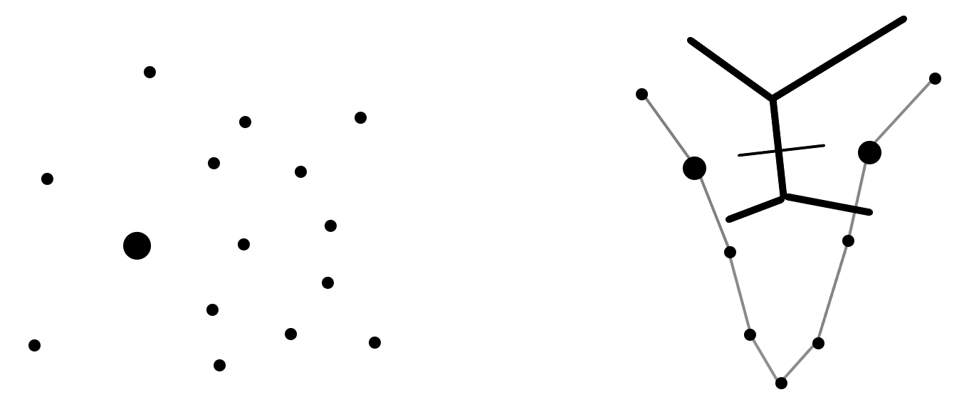
Figure 4: Typical problems associated to k-nearest neighbors (left) and Voronoi neighbors (right). On the left, most closest points to $v$ (in bold) are clustered at one side of it. On the right, vertices that are too far apart from each other belong to neighboring cells.

Therefore we merge these two criteria, and declare two points as neighbors when (i) each point is among the $k$-nearest neighbors of the other and (ii) their Voronoi cells in the decomposition of the ambient space $\mathbb{R}^{N}$ induced by $X$ are adjoining. In order to be efficient, inspired by sphere packing theory [[gensane2004dense]], we first choose a $k=12$ to compute the $k$-nearest points and then only keep as neighbors the vertices that are connected to $v$ in the Delaunay triangulation of these few points. Finally the relationship of neighborhood is made symmetric by reciprocating neighboring relationships where needed. The neighbors of $v$ will be denoted by $\operatorname{Neigh}(v)$. This produces a (locally non-planar) graph, which gives an idea of the local structure of $X$, but which will be in general very complicated.

4.2 Discrete curvature filter

In order to avoid the proliferation of critical points of the Morse-Smale function that in turn would generate a very high number of Morse cells, once we have identified neighbors of each point, we apply a discrete-curvature filter to the point-cloud. This means that we substitute each point $v$ for a weighted average of its position and the location of its neighbors:

$$h(v)=\alpha v+(1-\alpha)\frac{1}{|\operatorname{Neigh}(v)|}\sum_{v_{i}\in\operatorname{Neigh}(v)}v_{i}.$$

When applied a small number of times this filter defines a bijection between the original cloud and the filtered one, which preserves the topology of the underlying surface (see [[CraneCurvatureFlow]] for a thorough discussion of topology preserving curvature flows applied to triangle meshes). Hence, the decomposition we find for the filtered case will still be valid and topologically accurate for the original cloud. The application of this filter is not always needed, being most relevant when the point-clouds present a lot of noise or a high level of local variability.

4.3 Tangent space estimation

This task is performed through Principal Component Analysis [[Hoppe1992]]: if the point $v$ and all its neighbors $\operatorname{Neigh}(v)=\{v_{1},\dots v_{k}\}$ were co-planar we would have that for every $i$: $\langle\vec{vv_{i}},n_{j}\rangle=0$, where $n_{j}$ are all the normal vectors to the surface at $v$ (recall that in general we are in $\mathbb{R}^{N}$). Since in general this will not be the case, we find the $n_{j}$’s by minimizing the function $\sum_{j}\sum_{i=1}^{k}\langle\vec{vv_{i}},n_{j}\rangle^{2}$. This is equivalent to finding the regression plane through $v$ in the least squares sense, and it can be done efficiently by means of a singular value decomposition of the matrix with vectors $\vec{vv_{i}}$ as rows: the right singular vectors corresponding to the 2 largest singular values define the tangent plane, whereas the rest give us the normal directions.

4.4 Boundary recognition

Once we have an estimation of the tangent spaces, in principle a boundary point of the surface can be easily identified because after orthogonally projecting it and its neighbors on its tangent plane, they cluster in a semi-space (see the first panel of Figure 5). Nevertheless this method is difficult to implement robustly (see the second panel of Figure 5).

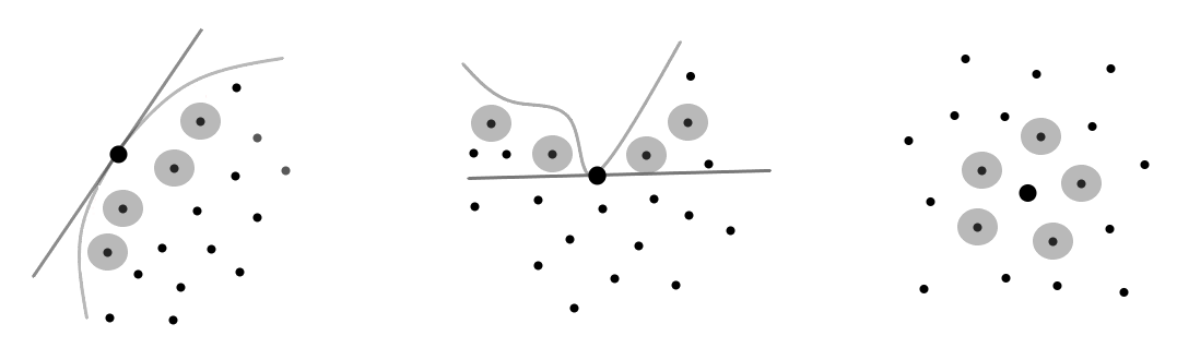
Figure 5: In principle, a boundary point can be identified easily because after projecting it and its neighbors on the tangent plane, they cluster in a semi-space of $\mathbb{R}^{2}$ (left panel). Nevertheless, this is not always the case for every boundary point (middle panel). To overcome this, we declare a point as being on the boundary when none of the plane projections of it and its neighbors in all their respective tangent planes enclose the point (right panel).

In order to obtain a robust detection, the idea will be to declare points as lying on the boundary only when the projections do not enclose the point. In points with high curvature where the tangent plane may not be perfectly estimated (or equivalently the normal vectors; for a discussion of this phenomenon, see [[NormalEstimation]]) the previous method can give false positives (see Figure 6 lower panel, left). In order to overcome this difficulty, we will also project the point and all its neighbors in the tangent planes estimated for the neighbors. We will build a graph for every projection and only declare $v$ as boundary point when none of the graphs enclose $v$ (see Figure 6 lower panel, right).

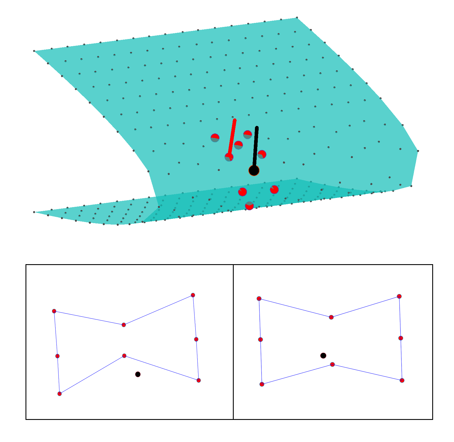
Figure 6: In interior points with high curvature the projections of the neighbors (red) of a point (black) into the tangent plane of the point may not enclose said point (lower panel, left). In order to avoid false positives we also project the point and its neighbors into the tangent planes estimated for the neighboring points (lower panel right).

Now we proceed to describe our method in detail: let $v\in X$, and $T_{v}S$ be the estimated tangent plane at $v$. We follow the following steps:

1. Given $\{v_{1},\dots v_{k}\}$ the neighbors of $v_{0}:=v$ we project the $k+1$ points on the planes $T_{v_{j}}S$ for $j=0,\ldots k$. These projections will be denoted by $\pi_{j}(v_{i})$.

2. We create a plane graph $G_{j}$ with the projected points for every $j=0,\ldots k$, where we add an edge between $\pi_{j}(v_{i})$ and $\pi_{j}(v_{l})$ only when $v_{i},v_{l}$ are themselves neighbors in the cloud and $i,l\neq 0$.

3. We declare the vertex $v_{0}$ as a boundary point only when none of the plane graphs $G_{j}$ enclose $\pi_{j}(v_{0})$ for every projection to $T_{v_{j}}S$.