Transformer In-Context Learning for Categorical Data
Abstract
Recent research has sought to understand Transformers through the lens of in-context learning with functional data. We extend that line of work with the goal of moving closer to language models, considering categorical outcomes, nonlinear underlying models, and nonlinear attention. The contextual data are of the form where each is drawn from a categorical distribution that depends on covariates . Contextual outcomes in the th set of contextual data, , are modeled in terms of latent function , where is a functional class with -dimensional vector output. The probability of observing class is modeled in terms of the output components of via the softmax. The Transformer parameters may be trained with contextual examples, , and the trained model is then applied to new contextual data for new . The goal is for the Transformer to constitute the probability of each category for a new query . We assume each component of resides in a reproducing kernel Hilbert space (RKHS), specifying . Analysis and an extensive set of experiments suggest that on its forward pass the Transformer (with attention defined by the RKHS kernel) implements a form of gradient descent of the underlying function, connected to the latent vector function associated with the softmax. We present what is believed to be the first real-world demonstration of this few-shot-learning methodology, using the ImageNet dataset.
1 Introduction
Large language models (LLMs) have demonstrated significant capabilities as few-shot learners [6]. To help understand this capability, recent work applied to functional data has shed light on the few-shot learning capabilities of Transformers, the technology that underpins most LLMs [2, 24, 8, 1, 3, 17, 13, 19, 25]. Such analysis of the Transformer is challenging. Consequently, much of that prior work has focused on real-valued observations, rather than categorical (of relevance for language modeling), and simplifications have often been made to the Transformer structure (for example, linear attention [2, 24, 1, 19]).
Prior to the introduction of the Transformer, the goal of teaching a model to learn based on a few functional-data examples was considered for many years, under several names: learning to learn, meta learning, and in-context learning, among others [20, 5, 4, 16, 10]. Often a model with parameters is assumed for input . Contextual data are considered, for different parameter settings, ; each is assumed drawn iid from a shared (and generally unknown) distribution . Given , the goal is to learn parameters that will serve as a good initialization when parameter refinement is done for any of the contexts . Given new context , where the outcomes are assumed generated by a function in the same class , ideally should serve as a good initialization from which are determined via model refinement using . Model agnostic meta-learning (MAML) is a seminal approach to this setup [10]. A key attribute of MAML, and most of its subsequent related approaches to meta learning [15], is that adaptation to is implemented by a form of model-parameter refinement, from .
In another line of research [20, 18], one seeks to learn a “meta model,” distinct from , and the meta model should (possibly implicitly) “learn to learn” new based on a small amount of contextual data, without refining the meta-model parameters. It has recently been recognized that the Transformer is a meta model in this class [24, 8, 1, 19, 25], where here the Transformer may be represented as , with parameters and representing a set of vectors connected to the contextual data (more details on this below). The Transformer implicitly learns to evaluate for specific (query) covariates , and adapt to a new context, but the function (and its parameters ) are not considered explicitly.
The Transformer parameters are learned based on a set of contextual examples , each with a different [24, 8, 1, 25]. Ideally, the Transformer learns to make an estimate of for the covariates in , and it predicts for a query . After training with , and learning an estimate of its parameters , given new context in the same functional class, but with parameters not seen before, the Transformer is to predict for query . The Transformer effectively performs model-parameter refinement in its forward pass, but without explicitly computing , and without refining the Transformer parameters .
Transformer-based in-context learning for functional data has been considered from two primary directions. One thread has examined what kind of functional classes can be handled by Transformer-based in-context learning [17]. In addition to making deterministic predictions of functional outcomes [17], Bayesian predictions have also been considered [14]. Moving beyond what types of functional data a Transformer can analyze in-context, a second thread has sought to understand how the Transformer performs functional few-shot learning [24, 8, 1]. Important insights have been made by simplifying the form of the underlying model and also simplifying the Transformer . Specifically, many recent studies have assumed the functional class consists of linear models [25, 24, 1], and the Transformer has been assumed to have linear attention (rather than the conventional softmax attention) [2, 24, 1, 19].
It has been shown that if is composed of linear functions and uses linear attention, then within its forward pass, each layer of the Transformer effectively implements a step of gradient descent (GD) refinement of from an initialization [2, 24, 1]. Early work showed that such a linear-attention Transformer design was theoretically possible, and empirically demonstrated it [24]; that work was followed by research showing that such a setup, and generalizations, are theoretically optimal for linear-class [1].
A Transformer with nonlinear attention is expected to be important when consists of nonlinear models. A natural generalization of inner-product-based (linear) attention is to consider inner products in a feature space , yielding Mercer-kernel-based attention. Transformers with Mercer kernel attention are applicable to function classes from the associated reproducing kernel Hilbert space (RKHS). This perspective has been developed recently, for real-valued observations [8].
With the goal of moving closer to language models, we here extend prior work to consider functional data for which each outcome is one of possible categories. Rather than observing samples of as in prior work [2, 24, 1], here is assumed to be a latent function, with real-valued outputs that feed into a softmax function to yield the probability of each category for input covariates .
We extend the aforementioned recent work on kernel-based attention [8] to the latent , with each component of modeled as being in an RKHS connected to the associated kernel attention. Through an extensive set of experiments with categorical observations, we demonstrate that a Transformer with nonlinear attention appears to be performing gradient descent in its forward pass, for the underlying . While many nonlinear kernel types are considered and generally perform well, we discuss important advantages of the softmax attention that underlies the original Transformer construction. Examples of this few-shot-learning framework are presented with the ImageNet dataset [9], believed to be the first real-world demonstration of the concepts developed here and in related literature [8, 24, 1].
2 Attention-Based Meta Learning
In Transformer-based in-context learning [2, 24, 1, 8], two models are considered: () , assumed responsible for generating the outcomes in the contextual data ; and () , a Transformer with parameters and with inputs defined by a sequence of vectors , encoding contextual data in as well as the query . We assume initially that , where is a deterministic function of , and in Section 3, this is extended to categorical outcomes which are probabilistically related to . We assume that may be nonlinear, and that it can be modeled as a member of an RKHS with specified kernel. Such an RKHS framing of the Transformer was first considered in [8].
We assume , where is an integer, and . The assumption that is a -dimensional real vector is meant as preparation for Section 3, where categorical observations are considered. Here the -dimensional real output vector is observed, where in Section 3 it will be latent, and will stipulate the probability of observed categorical data.
It has been shown [24, 1] that when is composed of linear models , with matrix model parameters playing the role of , an appropriately designed Transformer with linear attention can perform in-context learning on its forward pass. Each layer of the forward pass of the Transformer, with appropriate parameters , effectively implements one step of gradient descent (GD) for . The function is updated implicitly to via an attention layer, with this functional update performed for the covariates connected to , and for the new query . Following [8], we now extend this for nonlinear .
Consider linear models in a feature space specified by a given . Specifically, assume the function responsible for the data may be expressed as , where , now with , and . Using loss one can readily show (see the Appendix) that gradient descent (GD) dictates the following update rule at iteration :
| (1) |
where is a Mercer kernel, , is the sum of the two terms identified in (1) connected to the two attention heads, and is the learning rate. We identify contributions from two attention heads in (1), as below we show that this GD update can be implemented with an attention network that employs two attention heads. From (1), the GD update of the model parameters imposes that each component of resides in a reproducing kernel Hilbert space (RKHS) associated with kernel .
Note that in (1) we represent the GD-based update rule in terms of a possible Transformer design with two attention heads, and attention defined by the kernel (more on this below). In the Appendix we detail Transformer parameters that achieve this update, analogous to [24], but now applied to RKHS attention [8]. While this suggests that it is possible for a Transformer to implement GD on its forward pass, there may be other designs of the Transformer parameters that work well or even better for in-context learning when all Transformer parameters are trained based on data. As we demonstrate in extensive experiments, it appears that the Transformer does learn to do GD in its forward pass, consistent with (1).
We assume , where represents a -dimensional all-zeros vector; this corresponds to initializing the model parameters as and , also implying that, within (1), . In prior work [24], with linear functions (), the initial weight matrix was arbitrary, but the Transformer learning process effectively imposed that is an all-zeros matrix. Hence, the setting is consistent with prior work for linear models and linear attention, and extended here to kernel-based attention and inclusion of the bias term.
To underscore the connection to a Transformer, consider (1) represented by the sequence of operations at layer :
| (2) |
Transformer matrices , and can be designed to implement (2), as detailed in the Appendix.
At the left in (2) is shown the input vector at each position at layer . Masked attention is employed, in that input elements are used for keys and values, while all inputs at positions are used as queries. The output of the attention layer (center of (2)) manifests the negative of an incremental update to the predicted outcome, with this corresponding to one step of GD. On the right of (2), the input to the attention layer is added to the input, manifesting a skip connection. The last components of the result of this correspond to , where is the update the approximation of from the model.
At the first () layer of a Transformer implementation of (2), the input vectors at positions are , while at position the query is encoded as , corresponding to initially setting (which is to be predicted) as . At the last attention layer (the th layer, for an -layer model), the output vector associated with position is ; an inner product of this vector is performed with , yielding the predicted . Above we have considered a single covariate vector for which a prediction is made. As discussed when presenting results, it is possible to consider covariates for which predictions are made at once, and now Transformer queries are made with inputs , with the keys and values unchanged. At the output layer, the same linear prediction is performed using the outputs at positions .
Note that at each layer of the Transformer, two attention heads are employed, as indicated in (1). One of the attention heads implements kernel-based attention between the th query and th key, and the other attention head implements constant (equal to one) attention for each key-query pair. The constant attention is connected to estimating the bias of . The need for an attention head that yields constant attention has been discussed previously (see the Appendix of [26]), but constant attention is not possible with linear attention (i.e., when ). Introduction of a nonlinear kernel within the Transformer attention mechanism consequently has two advantages: () it allows modeling of nonlinear functions within the RKHS family; and () for proper setting of and and choice of kernel, it allows constant attention and bias term estimation (see the Appendix for details).
3 Categorical Outcomes
We now consider contextual data and a query with each , where is the number of categories. Functional class has a -dimensional real vector output, and will take the same form as considered in Section 2. However, here is latent, and the vector output specifies the probabilities of categories at a given covariate . Let represent output component of , and as a reference, we assume an additional component set as for all (in total there are components, and for , and accounts for the latter).
The probability that random variable equals when input random variable equals is modeled with the softmax function . Following the framework from the previous section, we specify , and . Using the cross-entropy loss with , a gradient-descent update of the model parameters yields the following sequential underlying-function update:
| (3) |
where , and represents component of , the latter a -dimensional vector with all components equal to zero, except at most a single 1 at component if ; corresponds to one-hot encoding, except that if the encoding makes an all-zeros vector.
Note the similarity of (3) to (1), although (3) is complicated by a mix of and , where (1) only involves the latter functional class. To address this, note that the softmax is a function of , and we approximate it with a first-order Taylor expansion about . For component of the softmax, this yields , where . Using this first-order approximation, the definition of and (3), we have
| (4) |
where we have used . In (4) we write equality, as this is the update rule used to implement the Transformer, but we underscore that approximations have been made to arrive at this expression: () linearization of the softmax about , and () has been approximated as a constant for all . We evaluate the impact of these approximations when presenting results in Section 4.
Consistent with initializing the parameters as and , for all , in (3), we have and . This is as in Section 2, where corresponded to the th component of the real-valued vector output. However, in (4) we are updating the components of the softmax function, and setting which corresponds to .
As alluded to above, the dependence of on component and covariates adds a complexity not present in the real-valued observations of Section 2. For simplicity, we treat as approximately constant for each , with that constant a function of gradient iteration (which translates to layer dependence in the Transformer). Combining that constant with the learning rate, we realize a learning rate that depends on the iteration and component . The component-dependent learning rate is a result of the aforementioned linearization, and it is consistent with generalizations of gradient descent, like Adam [12], that employ learning rates that are dependent on the component and change as the iterations of learning progress.
Given the similarity of (4) to (1), the former admits a Transformer-based update rule (through attention layers) analogous to (2). However, the following changes are implemented for categorical data: () for real-valued outcomes in (2), the input and output vectors employ the observed (in the contextual data) outcomes , whereas for categorical data these are replaced by -dimensional one-hot-like vectors , that encode the categorical data; () for categorical data we do not update the latent function whose components reside in an RKHS, we update the softmax function which is computed in terms of , and consequently while , we have within the Transformer , where is a ()-dimensional vector of all ones; and () for the categorical data we have a learning rate that depends in general on the attention layer and on the component of the softmax, . With these changes, the remaining characteristics of the Transformer construction are largely unchanged from real-valued observations, as detailed in the Appendix.
As discussed in Section 2 for real-valued outcomes, the approximate update rule in (4) suggests that the Transformer could perform nonlinear kernel-based GD of the underlying softmax function in its forward pass, with Transformer parameters consistent with (4), as discussed in the Appendix. A similar question holds for the categorical data which is the focus of this section. As demonstrated in Section 4, it appears, through extensive experiments, that the Transformer does indeed learn to implement GD of the underlying nonlinear function in its forward pass, consistent with (4).
We note categorical data were considered in [26], and a similar attention-based construction is developed for categorical data in the Appendix of [26] (see Eq. 2 there). However, in [26] the goal was to use the Transformer to update the model weights for categorical models, in a few-shot manner (effectively updating the weights of categorical model ). Here we are using a similar construction to directly predict via a Transformer, with no model-parameter fine-tuning or update.
In the Appendix we specify a construction for Transformer parameters that can implement the (approximate) GD updates reflected by (4). We compare the performance of our specified Transformer to a setup in which the parameters of are learned based on a set of categorical contextual data . While (4) is a result of gradient descent on a cross-entropy loss applied with the softmax function, (4) directly updates an approximation for for ; this is the output of softmax, and hence there is no additional softmax function applied to the output of the Transformer.
When learning all the Transformer parameters , the model output is fit to the vector (the one-hot-like encoding of the category for sample ). When training for , based on , the loss function is the distance between the true and the -dimensional vector output at position from the Transformer.
We emphasize that this learned Transformer is not the same as the setup in Section 2 from a key perspective: Here, at the input layer (layer ), the data at position are encoded as , emphasizing that because of the categorical data . This underscores that, like in Section 2, , but that this is then fed into the softmax to yield . In Section 2 the Transformer updates the model for , where for categorical data the Transformer updates the latent softmax function .
4 Experiments
We examine the performance of the Transformer models using synthetic as well as real-world data, considering categories within each context . Presenting first results for synthetic data, we consider two-dimensional covariates, i.e., , to aid visualization and interpretation (the subsequent real-world data discussed below considers ). The underlying code is applicable to an arbitrary number of categories and covariate dimension, and all software will be made available with the publication of the paper.
For each type of kernel attention, we will consider two ways to design the Transformer parameters. In the first method, which we refer to as “GD,” the model parameters are set as specified in Section 3 and detailed in the Appendix. In this setup, only the learning rate within the Transformer and the kernel parameter (detailed in the Appendix for each kernel type) are learned. The second method is referred to as “Trained TF,” in which all Transformer parameters are trained/learned. The training in both cases is performed with contextual data and it is evaluated on a separate contextual dataset . There are contextual pairs in each . For the synthetic data, like in [24], when training the Trained TF, we considered 5000 iterations of Adam [12] using and for each iteration. When learning the kernel parameter and learning rate for GD, we also trained for 5000 iterations, using and each iteration. The performance of the Trained TF and GD models were assessed by averaging over 10,000 different sets of contextual data (10,000 different instantiations of ). For Trained TF, we consider 5 different random initializations of the model parameters, and below we show average results for each of these random seeds, to give a sense of learning stability. All computations were performed on a single 16GB NVIDIA V100 GPU.
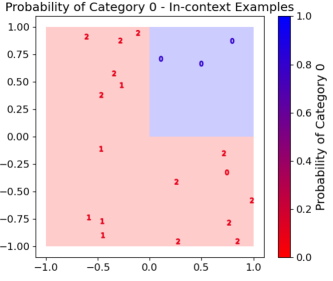
As discussed in Section 3, an underlying softmax function is associated with the data generation. For a small number of contextual samples , as we consider in our examples, many different underlying could give give rise to the same observed categorical data. Through extensive experimentation, we have found it helpful to make the synthetic-data-generation process as simple as possible. Specifically, like [24] each of the two components of is assumed drawn iid, uniform over . Given a generated 2D covariate vector, the category probabilities are defined by the quadrant in which the covariates reside as shown in Figure 1.
To enhance visualization of the Transformer predictions, we first consider many queries, , for context , so we can observe the predicted across the entire covariate space. Specifically, here we consider (10,000) queries uniformly positioned across the 2D covariate space. Importantly, all of these queries are analyzed at once, via a single forward pass of the Transformer.
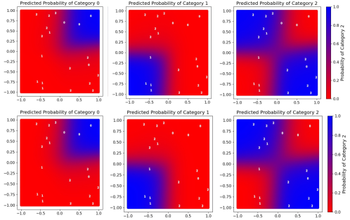
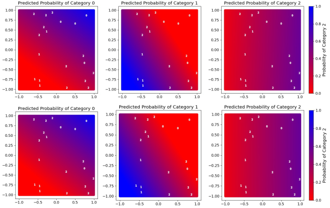
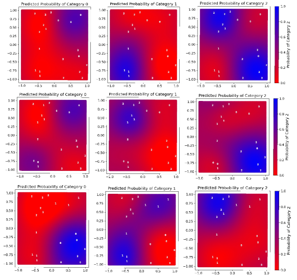
In Figure 2 we consider results from the Transformer, for the contextual data depicted in Figure 1, for the softmax attention kernel (, with a parameter to be learned). Note that this kernel is not a Mercer kernel, but the Transformer performed well nevertheless. The close agreement between the results in the first and second row suggests that the fully-trained Transformer is learning to perform GD in the forward pass, based on observed context.
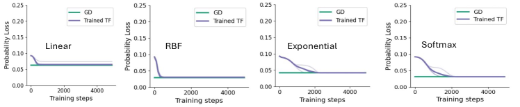
In the Appendix we present additional results in the same form as Figure 2, for the linear, RBF, exponential and Laplacian attention kernels. Examination of those results indicate: () close agreement between the GD and Trained TF, for a single attention layer and one attention head; () all of the nonlinear kernels effectively capture the nonlinear decision surfaces associated with the data, but the detailed way (degree of smoothness) varies between kernels; () the linear kernel cannot model the nonlinear decision surfaces, but yields linear decision surfaces that are often effective, albeit slightly less accurate; () the normalization associated with the softmax kernel seems to yield very stable training of the model, compared to training with exponential-kernel-based attention, which has the same form apart from the normalization.
For the same class of synthetic data, in Figure 3 we compare the performance of the Transformer as designed in Section 3 (again, termed GD) with a Transformer for which all parameters are designed (termed Trained TF). For the Trained TF, we show the MSE as a function of the learning iteration (on a separate test dataset, as discussed above), and compare performance with GD. In all cases a single attention head is employed and one layer of attention is considered. We observe that after a sufficient number of training iterations (steps) for Trained TF, there is very close agreement with the GD-designed Transformer. Consistent with all results presented thus far, this suggests that the fully trained Transformer is learning to perform GD in its forward pass.
As discussed in Section 3, multiple attention heads allow consideration of a bias term in . To explore this, within the fully trained Transformer (Trained TF) we moved beyond the single attention head, considering up to four different attention heads. We compare results of those Transformers to the GD transformer with one attention head (as a reference, to examine the degree to which bias impacts the model). As shown in the left of Figure 4, for the softmax kernel attention, up to four fully-trained heads yield performance very close to that of the designed GD-based Transformer with a single head (when one attention head is used in the Trained TF, the model converges to the GD Transformer results). This indicates that the impact of the bias term is small, as expected, given the data-generation process. We also augmented data generation, to impose more bias, but we found that results with one or two attention heads were similar. We speculate that with small context size, like the considered here, the impact of bias on the model is small unless the bias is substantial. We observed similar phenomena when considering real-valued data as discussed in Section 2, the results of which are omitted for brevity. These results indicate that the flexibility of the RKHS model is sufficient to model data without a bias term (i.e., with one attention head), for relatively small context sizes.
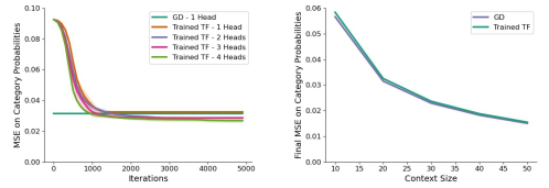
A question of interest is whether a Transformer trained using data with context may be applied to data with context size . Examining (4), we observe that the context size appears as a factor in the update equation for the model. We found that for all attention kernels other than softmax, the software could be applied to arbitrary context size , as long as the scaling in the code is adjusted to . However, the need to adjust the underlying software for different context sizes is inconvenient. A very important observed property of the Transformer with softmax attention is that a model trained with context size can be applied without change for arbitrary context size . This is a result of the normalization within the softmax attention, which yields performance invariant to change in .
Using the synthetic data, in Figure 4 (right), we compare the performance of the GD and Trained TF designs with softmax attention, when learning was done with context size , and the models are applied to new contextual data with varying from to , with no change to any Transformer parameters. We here consider one attention head, and one attention layer. We note the near exact agreement between the fully-trained and GD-designed Transformers, and that as increases the accuracy of the model improves (MSE computed at the centers of the four quadrants, see Figure 1).
In all experiments presented above, we have considered a single attention layer, and the Transformer was found to yield a good approximation to . We also considered additional experiments, where the number of attention layers were greater than one, and each layer had separately learned parameters (for the GD Transformer, only the learning rates were learned at the different layers, with the kernel parameter shared). We found that the results did not change significantly with more than one attention layer, with detailed results omitted for brevity. We did note differences in the training properties of the different kernels for Trained TF, and multiple attention layers were considered. For example, the learning process for the exponential kernel could be unstable, but the softmax-based attention (which is an exponential kernel plus normalization) trained in a very stable manner, with increasing layer number. In all of our experiments, we found the softmax-based attention yielded accurate nonlinear models and and trained very effectively.
Our final experiment involves real data, from the ImageNet dataset [9]. Each image from this dataset is analyzed by the VGG deep CNN [22], yielding 512 feature maps at the final layer. The features from each of these feature maps are then averaged. Consequently, image is represented by VGG-generated covariates . We show results for the GD-based Transformer discussed in Section 3, for which we only learn the kernel parameter (absent for the linear kernel) and the Transformer learning rate. We consider one attention head and one attention layer.
There are 1000 image classes (labels) in the ImageNet dataset. Each contextual set is designed so as to be composed with data from three image classes, selected uniformly at random, with 10 examples per class, also selected uniformly at random. This yields contextual data of size . The Transformer makes a prediction for , which has a label among the three in . To learn the small number of parameters associated with the GD Transformer models, the used for training employ 900 of the label types, and we evaluate performance for associated with held-out label types from among the remaining 100 classes. Consequently, this is a real-world example of few-shot learning: when testing, the Transformer is presented with contextual examples of data types it has not seen before, and it is then asked to classify as one of these new label types.
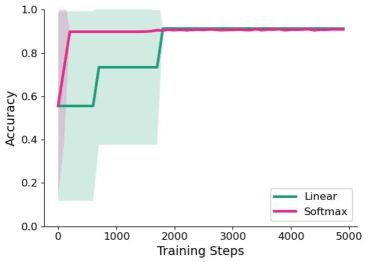
Since the deep VGG model has already extracted rich features at its output layer, we expect the linear-attention Transformer to be as effective as the nonlinear-kernel Transformer. In Figure 5 we show prediction accuracy results of the most probable predicted label, as a function of learning step. After sufficient training steps, the most-probable label typically had a probability near 0.9, reflecting a high-confidence prediction.
As expected, the results of linear and softmax attention in Figure 5 are similar with a sufficient number of training iterations (training is performed using Adam [11] with batch size 512), but the softmax attention converges much faster. This suggests that the features from the VGG are separable by a linear classifier, but the training of the Transformer to do this well, in a few-shot setting, is more difficult with linear attention than doing few-shot learning with softmax-based attention. After 5000 training steps the linear and softmax attention Transformers perform almost identically on this few-shot-learning task, with correct label classification probability 0.91, and with variation less than 0.001 on different splits of train and test.
5 Conclusions
The Transformer network has been examined for in-context learning with functional data, considering categorical outcomes, nonlinear underlying models, and nonlinear attention. Extensive analysis and results indicate, consistent with prior work but now for categorical data, that the Transformer implements a form of functional gradient descent in its forward pass, here on a latent function. We have demonstrated these concepts with simulated and real-world data, the latter applied to the ImageNet dataset, that shows the capacity of this framework to effectively perform few-shot learning on the Transformer forward pass (no model-parameter refinement).
References
- [1] K. Ahn, X. Cheng, H. Daneshmand, and S. Sra. Transformers learn to implement preconditioned gradient descent for in-context learning, 2023.
- [2] K. Ahn, X. Cheng, M. Song, C. Yun, A. Jadbabaie, and S. Sra. Linear attention is (maybe) all you need (to understand transformer optimization), 2024.
- [3] E. Akyörek, D. Schuurmans, J. Andreas, T. Ma, and D. Zhou. What learning algorithm is in-context learning? investigations with linear models. International Conference on Learning Representations, 2022.
- [4] M. Andrychowicz, M. Denil, S. Gomez, M.W. Hoffman, D. Pfau, T. Schaul, and N. de Freitas. On the optimization of a synaptic learning rule. Neural Information Processing Systems, 2016.
- [5] S. Bengio, Y. Bengio, J. Cloutier, and J. Gecsei. On the optimization of a synaptic learning rule. Optimality in Artificial and Biological Neural Networks, 1992.
- [6] T.B. Brown, B. Mann, N. Ryder, M. Subbiah, J. Kaplan, P. Dhariwal, A. Neelakantan, P. Shyam, G. Sastry, A. Askell, S. Agarwal, A. Herbert-Voss, G. Krueger, T. Henighan, R. Child, A. Ramesh, D.M. Ziegler, J. Wu, Cl. Winter, C. Hesse, M. Chen, E. Sigler, M. Litwin, S. Gray, B. Chess, J. Clark, C. Berner, S. McCandlish, A. Radford, I. Sutskever, and D. Amodei. Language models are few-shot learners. CoRR, abs/2005.14165, 2020.
- [7] C. Chen and O.L. Mangasarian. A class of smoothing functions for nonlinear and mixed complementarity problems. Computational Optimization and Applications, 1996.
- [8] X. Cheng, Y. Chen, and S. Sra. Transformers implement functional gradient descent to learn non-linear functions in context, 2024.
- [9] J. Deng, W. Dong, R. Socher, L.-J. Li, K. Li, and F.-F. Li. ImageNet: A large-scale hierarchical image database. Conference on Computer Vision and Pattern Recognition, 2009.
- [10] C. Finn, P. Abbeel, and S. Levine. Model-agnostic meta-learning for fast adaptation of deep networks, 2017.
- [11] D. Kingma and J. Ba. Adam: A method for stochastic optimization. In ICLR, 2015.
- [12] D.P. Kingma and J. Ba. Adam: A method for stochastic optimization, 2017.
- [13] A. Mahankali, T.B. Hashimoto, and T. Ma. One step of gradient descent is provably the optimal in-context learner with one layer of linear self-attention. arXiv:2307.03576, 2023.
- [14] S. Muller, N. Hollmann, S. Pineda, J. Grabocka, and F. Hutter. Transformers can do Bayesian inference. International Conference on Learning Representations, 2022.
- [15] A. Nichol, J. Achiam, and J. Schulman. On first-order meta-learning algorithms, 2018.
- [16] S. Ravi and H. Larochelle. Optimization as a model for few-shot learning. International Conference on Learning Representations, 2017.
- [17] P.S. Liang S. Garg, D. Tsipras and G. Valiant. What can transformers learn in-context? a case study of simple function classes. Advances in Neural Information Processing Systems, 2022.
- [18] A. Santoro, S. Bartunov, M. Botvinick, D. Wierstra, and T. Lillicrap. Meta-learning with memory-augmented neural networks, 2016.
- [19] I. Schlag, K. Irie, and J. Schmidhuber. Linear transformers are secretly fast weight programmers. International Conference on Machine Learning, 2021.
- [20] J. Schmidhuber. Evolutionary principles in selfreferential learning. on learning how to learn. Diploma thesis, Institut f. Informatik, Tech. Univ. Munich, 1987.
- [21] B. Schölkopf and A.J. Smola. Learning with kernels: support vector machines, regularization, optimization, and beyond. MIT press, 2002.
- [22] K. Simonyan and A. Zisserman. Very deep convolutional networks for large-scale image recognition, 2015.
- [23] Ashish Vaswani, Noam Shazeer, Niki Parmar, Jakob Uszkoreit, Llion Jones, Aidan N. Gomez, Lukasz Kaiser, and Illia Polosukhin. Attention is all you need, 2023.
- [24] J. von Oswald, E. Niklasson, E. Randazzo, J. Sacramento, A. Mordvintsev, A. Zhmoginov, and M. Vladymyrov. Transformers learn in-context by gradient descent, 2023.
- [25] R. Zhang, S. Frei, and P.L. Bartlett. Trained transformers learn linear models in-context. arXiv:2306.09927, 2023.
- [26] A. Zhmoginov, M. Sandler, and M. Vladymyrov. Hypertransformer: Model generation for supervised and semi-supervised few-shot learning. International Conference on Machine Learning, 2022.
Appendix A Review of Transformer Construction for Real Vector Outcome
The Transformer has been developed previously [24] for linear attention and linear models, which is readily extended for in-context functional learning with Mercer kernels, as discussed in Section 2. We leverage the recently developed extension to nonlinear models and kernel-based attention developed in [8]. We briefly summarize that prior work, including how the Transformer parameters are set to implement gradient descent (GD). Specifically, we demonstrate the GD update in (1), which we repeat here for convenience:
| (5) |
can be implemented via the mechanism in (2), also repeated here as
| (6) |
From (6), the input at position of the Transformer at attention layer is , and at the first layer () this corresponds to , as . At position , corresponding to the query, is initialized at (it is which will be estimated at the output of the network).
Starting with the first attention head in (5), the key and query projection matrices are
| (7) |
and the value projection matrix is
| (8) |
where is the identity matrix, and is the all-zeros matrix.
Using the construction without preconditioning, and . The keys and values correspond to vectors , and the queries to . This is equivalent to masked (applied to the keys) attention on all vectors, with mask weights of 1 on the first vectors (the labeled samples), and a mask weight of zero on the vector (the unlabeled query).
For the first attention head in (5), the query and keys are used within a kernel with any Mercer kernel applicable. The output of position for attention head 1 at layer is
| (9) |
where , and is defined by for .
The second attention head in (5) employs the same as the first head, but now the matrices and must be designed so as to yield a constant kernel output for all and (one could also have a constant output other than 1). How this is achieved depends on the kernel.
The family of Mercer kernels are widely known, examples of which (and that we consider in experiments) are [21]
-
•
Linear:
-
•
Radial basis function (RBF):
-
•
Laplacian:
-
•
Sigmoid:
-
•
Polynomial:
-
•
Cosine:
-
•
Chi-squared:
For the RBF, Laplacian and Chi-squared kernels, a constant kernel output is achieved if and are all-zeros matrices, from which . For the sigmoid and polynomial kernels, constant output is achieved if and/or are all-zeros matrices. Note that the sigmoid kernel is not technically Mercer, however, it has been demonstrated to work well in practice [21]. For the linear and cosine kernels, in the absence of additional elements to the Transformer (e.g., positional embeddings), it does not appear that and can be designed to achieve constant (and non-zero) outputs for all and . For this reason, when considering estimation of the bias term , we do not consider linear or cosine kernels.
This construction of and connected to the bias term was also discussed in [26] (see the Appendix of that paper). However, in [26], the original softmax attention was used, rather than a Mercer kernel construction. Because of the construction of the softmax, also yields constant attention, where the constant is , where is the number of keys.
For each query input to layer , there is an output from head 1, and similarly is output from head 2. With a skip connection, the total output from attention layer is (right in (6))
| (10) |
where and . The term corresponds to the middle of (6). Since the first components of and are zeros, the first columns of and are arbitrary. For simplicity, we define and , where it is assumed that the constant output of the kernel associated with head 2 is one.
Appendix B Categorical data
For convenience, we repeat the update rule (4) for categorical data:
| (11) |
The Transformer implementation of this update rule proceeds as in Section A, with the following changes: () The categorical outcomes are encoded by the one-hot-like vector ; () the initialization is employed; and the learning rate at layer is in general a function of component .
Appendix C Additional Results
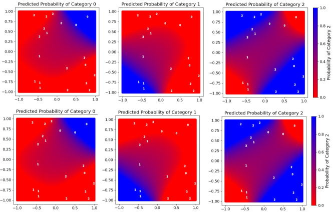
In Figure 6 we consider the same setup as in Figure 2, but now for radial basis function (RBF) kernel attention. All the results in Figure 6 correspond to the “GD” model developed in Section 3. Similar close correspondence is observed between the GD and Trained TF versions of the RBF-based Transformer, with the latter omitted for brevity. The top row of Figure 6 considers the same contextual data as in Figure 2. The second and third rows in Figure 6 consider the same GD Transformer model, but different examples of . The results in the three rows show the ability of the Transformer to adapt in the inference phase (forward pass) to new contextual data , with no change in model parameters.
Comparing Figure 2 with the top row of Figure 6 (for which is the same), we note that the Transformers with softmax and RBF attention, respectively, give similar inferences of , but that the form of the RBF yields a smoother representation more closely tied to the observed samples. We do not expect the Transformer to recover the exact shape of the underlying (as discussed wrt with Figure 1) with only contextual examples (although the form of the softmax kernel does do a bit better for this case). We have observed that with increasing context size the inferred more closely follows the underlying form of the generation process in Figure 1.
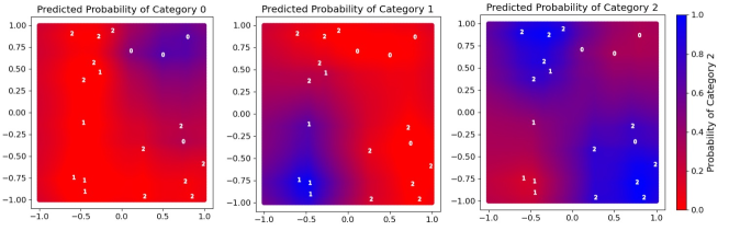
In Figure 7 we show results for a linear kernel. The linear-attention Transformer is unable to capture the nonlinear structure of , as expected. However, examination of Figure 7 shows that the linear-attention Transformer does infer a model that fits the contextual data reasonably well (albeit in a linear manner). In Figure 3 we showed that while the predictions of the linear model are inferior to the nonlinear attention results, they are still reasonably good. This underscores the importance, we feel, of visualizing the data, the structure of which plays an important role in the relative efficacy of linear vs. nonlinear attention.
From Figure 7, note that the linear-attention model is not able to infer the nonlinear structure of the categorical probabilities as a function of covariate position. We note, however, close agreement between the predictions of the GD-based designed Transformer (top row in Figure 7) and the Trained TF for which all model parameters are trained based on contextual examples (bottom row in Figure 7).
Examining Figure 7 carefully, across a given row, the left-most figure puts high probability mass near contextual samples with label 0, the center image does the same for contextual data with label 1, and finally the right figure (mostly) puts high probability mass near contextual samples with label 2. The probability of label 2 has the most nonlinear character as a function of covariates (see Figures 2 and 6), and it is this distribution (right-most figure in each row of Figure 7) that is most mismatched to the data for the linear-attention model. Nevertheless, overall (and particularly for labels 0 and 1) the linear-attention model does do a reasonably good job of fitting the contextual data, albeit in a linear manner. This explains why the linear-attention model does perform relatively well in Figure 3, albeit not as good as the nonlinear-attention models.
Analysis of this sort highlights the importance of carefully visualizing the data. Even if the used to generate data is nonlinear, depending on the size of , the observed categorical data may be fit relatively well by a linear model, making it appear that nonlinear attention is unimportant (but such conclusions are very data-dependent). The importance of understanding the properties of the data is why we considered the relatively simple and robust data-generation process summarized in Figure 1, and the low-dimensional covariates (), as it allows us to assure (by visualization) that the observed contextual data are actually nonlinear in their distribution, and to visualize differences between predictions of linear and nonlinear attention models.
In Figures 8 and 9 we consider the same contextual data as considered in Figure 7, but now for an exponential kernel and a Laplacian kernel, respectively. The exponential kernel was considered in [8], specifically , where is a parameter to be learned. These results are based on the construction in Section 3 (termed GD), in which only the learning rate within the Transformer and the kernel parameter are learned.
We found that the training of all model parameters (Trained TF) was unstable when considering attention with the Laplacian kernel, likely because of the non-differential nature of the norm within the kernel. There are many methods that have been developed to address the non-differential character of this norm [7], which may be considered in future work for this attention model. However, we have noted the multiple respects with which the softmax kernel and associated attention are attractive (e.g., robustness to variable context size). Therefore, in practice there will typically be little reason to consider the Laplacian kernel within an attention model, which is presented here for comparison. We note that all of the nonlinear kernels perform similarly (but distinctly) in representing the nonlinear structure of the underlying probability of categories, as a function of covariates.
Concerning the exponential kernel, we found that the training process of the Trained TF (all parameters trained) could become unstable numerically when the number of attention layers increased. By contrast, as the number of attention layers increased, the Transformer with softmax attention performed in a stable manner when training for all model parameters; this is important, as the softmax attention is just a normalized version of exponential-kernel-based attention. This appears to underscore the importance of the normalization within the softmax attention (helps with numerical stability when training), and possibly also sheds light on the importance of normalization in other parts of the original Transformer architecture [23].