A general model for spin coating on a non-axisymmetric curved substrate

Abstract

We derive a generalised asymptotic model for the flow of a thin fluid film over an arbitrarily-parameterised non-axisymmetric curved substrate surface based on the lubrication approximation. In addition to surface tension, gravity, and centrifugal force, our model incorporates the effects of the Coriolis force and disjoining pressure, together with a non-uniform initial condition, which have not been widely considered in existing literature. We use this model to investigate the impact of the Coriolis force and fingering instability on the spreading of a non-axisymmetric spin-coated film at a range of substrate angular velocities, first on a flat substrate, and then on parabolic cylinder- and saddle-shaped curved substrates. We show that, on flat substrates, the Coriolis force has a negligible impact at low angular velocities, and at high angular velocities results in a small deflection of fingers formed at the contact line against the direction of substrate rotation. On curved substrates, we demonstrate that as the angular velocity is increased, spin coated films transition from being dominated by gravitational drainage with no fingering to spreading and fingering in the direction with the greatest component of centrifugal force tangent to the substrate surface. For both curved substrates and all angular velocities considered, we show that the film thickness and total wetted substrate area remain similar over time to those on a flat substrate, with the key difference being the shape of the spreading droplet.

1 Introduction

Spin coating is widely used to apply functional and protective coatings in the manufacturing of electronic and optical components, such as microprocessors, light-emitting diode displays, and solar panels. The spin coating process consists of depositing a coating liquid onto a substrate surface, then rotating the substrate at high speed so that centrifugal force spreads the liquid over the surface (Cohen & Lightfoot, 2011). Once the liquid has formed a thin film over the entire substrate surface, the film is allowed to cure by solvent evaporation, photochemical, or other means, to leave a uniform and highly-reproducible coating. Current spin coating techniques, however, are unable to reliably produce uniform coatings on curved substrates (Rich et al., 2021). This restricts a wide range of spin-coated products to only flat geometries or singly-curved surfaces (by bending flat surfaces without stretching).

Emslie et al. (1958) developed a simple one-dimensional model for the dynamics of an axisymmetric thin fluid film on a rotating flat substrate, based on the lubrication approximation, considering only the effects of centrifugal force. They showed that, regardless of the initial film profile, a spin coated film on a flat substrate will tend towards a uniform coating. Models for spin-coated films have since been extended to incorporate additional effects such as gravitational and Coriolis forces, surface tension, and curved substrate geometry. The case when surface-tension and moving-contact-line effects are significant on flat substrates was later studied by Wilson et al. (2000). Chen et al. (2009) and Liu et al. (2017) presented one-dimensional models to predict the thickness of spin-coated films on convex spherical substrates, and demonstrated close agreement with the thickness of experimentally-measured films. Kang et al. (2016) and Duruk et al. (2021) used similar models to investigate the flow of a film over the entire surface of rotating spherical and spheroidal substrates, paying particular attention to the film dynamics during the transition from gravity- to centrifugal force-driven flow as the angular velocity of the substrate is increased. Finally, these one-dimensional models were generalised by Weidner (2018) to allow for an arbitrary axisymmetric substrate, such as with ridges and dips.

All of the above models have only considered the flow of axisymmetric films, and cannot capture the more complex dynamics which occur in non-axisymmetric flows, such as fingering instabilities, as observed experimentally by Fraysse & Homsy (1994), and angular velocity components introduced by the Coriolis force. In the case of an axisymmetric film, Myers & Charpin (2001) showed that the effects of the Coriolis force would have no impact on film thickness, but would induce an angular velocity component that could affect the evolution of non-axisymmetric films. This was supported by experiments by Cho et al. (2005) demonstrating the deflection of fingers formed at the contact line due to the Coriolis force. On a flat substrate, spreading from a droplet initial condition was investigated by Schwartz & Roy (2004) without assuming an axisymmetric flow and including the Coriolis force, where they were able to reproduce the fingering instability observed by Fraysse & Homsy (1994) as well as finger deflection similar to Cho et al. (2005), but only while using a viscosity 14 times smaller than used in experiments.

Better understanding the dynamics of thin liquid films on stationary curved substrates has been the topic of several studies starting with the work of Schwartz & Weidner (1995) who included the effects of substrate curvature in the lubrication approximation for planar flows. The effects of inertia were later considered in Ruschak & Weinstein (2003) for a two-dimensional flow. For the three-dimensional flow of a thin liquid film on a stationary curved substrates, a general theory for thin films driven by surface tension and gravity was developed by Roy et al. (2002) and Thiffeault & Kamhawi (2006), allowing for flow to be modelled on any smooth substrate geometry, and using any parameterisation of the substrate geometry. The possible inclusion of solidification in the governing equations was concurrently considered in Myers et al. (2002) and the inertia effects later included in Wray et al. (2017). This general framework was later used by Takagi & Huppert (2010), Balestra et al. (2016, 2018), Qin et al. (2021), Ledda et al. (2022), and McKinlay et al. (2023) to study gravitational drainage and contact-line instabilities over a range of curved substrate geometries. The general theory was extended by Mayo et al. (2015) to simulate the dynamics of droplets on leaves (with the addition of disjoining pressure at the contact line).

Since the pioneering work of Howell (2003), few studies have considered the combined effects of a non-trivial substrate kinematics with a complex substrate shape. A notable exception which builds on the large body of literature related to rimming flows on circular cylinder—see for example Evans et al. (2004); Rietz et al. (2017); Lopes et al. (2018); Mitchell et al. (2022)—is the work in Li et al. (2017) investigating the free-surface dynamics of a thin film on a rotating elliptical cylinder. Recently, Duruk et al. (2023) modelled coating flows on rotating ellipsoids (with the addition of centrifugal force, but not the Coriolis force).

We aim, in this work, to extend these models by presenting an extended general theory which includes all non-inertial forces and therefore can reliably simulate spreading from a droplet initial condition over a rotating, non-axisymmetric curved substrate and shed light on the combined effects of rotation and substrate curvature on the film spreading dynamics. We also aim to clarify to which extent the Coriolis force which has commonly been assumed (and convincingly been demonstrated) to be negligible for axisymmetric thin film flow configurations can still be ignored for non-axisymmetric surfaces. This has remained, to the best of the authors’ knowledge, an open question.

In section 2, we will derive a dimensionless general lubrication model for the evolution of a thin fluid film over the surface of an arbitrarily-parameterised rotating curved substrate following a similar methodology to Roy et al. (2002) and Thiffeault & Kamhawi (2006), incorporating the effects of surface tension, disjoining pressure, gravity, centrifugal, and Coriolis forces.

Section 3 gives the parameters and numerical details used to implement this model. In section 4, we present the results from a series of example simulations. In section 4.1, we first consider the spreading of a spin-coated droplet on a flat substrate in order to demonstrate the effects of the Coriolis force at different angular velocities. In section 4.2, we then show the effect of two different non-axisymmetric curved substrates (a parabolic cylinder and saddle) on the spreading of a spin-coated droplet and the onset of the fingering instability in gravity-driven, transitional, and centrifugal force-driven flow regimes. Finally, in section 4.3, we present quantitative results comparing the rate of film spreading over the different substrate geometries.

2 Model

2.1 Substrate-based curvilinear coordinate system

Consider a thin film of an incompressible Newtonian fluid on a smooth substrate surface. Let the substrate surface, $\boldsymbol{s}(x^{1},x^{2})$, be a two-dimensional Riemannian manifold parameterised by $(x^{1},x^{2})\in\mathbb{R}^{2}$. Let

$$\boldsymbol{e}_{\alpha}=\frac{\partial\boldsymbol{s}}{\partial x^{\alpha}},\qquad\hat{\boldsymbol{n}}=\frac{\boldsymbol{e}_{1}\times\boldsymbol{e}_{2}}{\big{\lVert}\boldsymbol{e}_{1}\times\boldsymbol{e}_{2}\big{\rVert}},$$ (1)

be basis vectors tangent to the substrate (for $\alpha\in\{1,2\}$, as with other Greek indices throughout), and a unit vector in the positive normal direction to the substrate, respectively. Note that $\boldsymbol{e}_{\alpha}$ are not necessarily orthogonal or normalised, and a suitable choice of substrate parameterisation is required to ensure the desired surface orientation. We also define cobasis vectors such that $\boldsymbol{e}_{\alpha}\boldsymbol{\cdot}\boldsymbol{e}^{\beta}=\delta_{\alpha}{}^{\beta}$ (where $\delta_{\alpha}{}^{\beta}$ is the Kronecker delta) and $\boldsymbol{e}^{\alpha}\boldsymbol{\cdot}\hat{\boldsymbol{n}}=0$:

$$\boldsymbol{e}^{1}=\frac{\boldsymbol{e}_{2}\times\hat{\boldsymbol{n}}}{\big{\lVert}\boldsymbol{e}_{1}\times\boldsymbol{e}_{2}\big{\rVert}},\qquad\boldsymbol{e}^{2}=\frac{\hat{\boldsymbol{n}}\times\boldsymbol{e}_{1}}{\big{\lVert}\boldsymbol{e}_{1}\times\boldsymbol{e}_{2}\big{\rVert}}.$$ (2)

Let $h(x^{1},x^{2},t)$ be the thickness of the fluid film above $\boldsymbol{s}(x^{1},x^{2})$ at time $t$, measured in the positive normal direction to the substrate surface. Each point in the fluid film can then be written as

$$\boldsymbol{r}(x^{1},x^{2},n)=\boldsymbol{s}(x^{1},x^{2})+n\hat{\boldsymbol{n}}(x^{1},x^{2}),$$ (3)

where $0\leq n\leq h$ is the distance from the substrate surface. This coordinate system is shown in figure 1.

Figure 1: The substrate surface and coordinate system, together with the basis vectors, $\boldsymbol{e}_{1}$, $\boldsymbol{e}_{2}$, and unit normal vector, $\hat{\boldsymbol{n}}$, at the point $\boldsymbol{s}(x^{1},x^{2})$.

Let $\mathsfbi{G}$ be the metric tensor on the substrate surface with components

$$G_{\alpha\beta}=\boldsymbol{e}_{\alpha}\boldsymbol{\cdot}\boldsymbol{e}_{\beta},\qquad G^{\alpha\beta}=\boldsymbol{e}^{\alpha}\boldsymbol{\cdot}\boldsymbol{e}^{\beta}.$$ (4)

Distance and area elements on the substrate surface can then be written as

$$(\mathrm{d}s)^{2}=G_{\alpha\beta}\,\mathrm{d}x^{\alpha}\mathrm{d}x^{\beta},\qquad\mathrm{d}A=\sqrt{G}\,\mathrm{d}x^{1}\mathrm{d}x^{2},$$ (5)

adopting the Einstein summation convention for repeated Greek indices, where $G=\det(\mathsfbi{G})=G_{11}G_{22}-(G_{12})^{2}$ is the determinant of the metric. Now, let

$$K_{\alpha}{}^{\beta}=\frac{\partial\boldsymbol{e}^{\beta}}{\partial x^{\alpha}}\boldsymbol{\cdot}\hat{\boldsymbol{n}}$$ (6)

define the symmetric substrate curvature tensor, $\mathsfbi{K}=K_{\alpha}{}^{\beta}\boldsymbol{e}^{\alpha}\boldsymbol{e}_{\beta}$. We can obtain the components $K_{\alpha\beta}=G_{\beta\gamma}K_{\alpha}{}^{\gamma}$ and $K^{\alpha\beta}=G^{\gamma\beta}K_{\gamma}{}^{\alpha}$ by the usual way of raising and lowering indices with the metric. We define the mean curvature and Gaussian curvature of the substrate, respectively, as follows:

$$\kappa=\mathrm{tr}(\mathsfbi{K})=K_{\alpha}{}^{\alpha},\qquad K=\det(\mathsfbi{K})=K_{1}{}^{1}K_{2}{}^{2}-K_{1}{}^{2}K_{2}{}^{1}.$$ (7)

Accounting for curvature, the basis and cobasis tangent vectors can be extended to the space around the substrate:

$$\boldsymbol{e}^{+}_{\alpha}=\frac{\partial\boldsymbol{r}}{\partial x^{\alpha}}=\boldsymbol{e}_{\alpha}-nK_{\alpha}{}^{\beta}\boldsymbol{e}_{\beta},\qquad\boldsymbol{e}^{+\alpha}=\boldsymbol{e}^{\alpha}+nK_{\beta}{}^{\alpha}\boldsymbol{e}^{\beta}+O(n^{2}),$$ (8)

so that $\boldsymbol{e}^{+}_{\alpha}\boldsymbol{\cdot}\boldsymbol{e}^{+\beta}=\delta_{\alpha}{}^{\beta}+O(n^{2})$. This leads to an extended metric tensor parallel to the substrate surface, $\mathsfbi{G}^{\,+}$, with components

$$\left.\begin{array}[]{c}G^{+}_{\alpha\beta}=\boldsymbol{e}^{+}_{\alpha}\boldsymbol{\cdot}\boldsymbol{e}^{+}_{\beta}=G_{\alpha\beta}-2nK_{\alpha\beta}+O(n^{2}),\\[4.0pt] G^{+\alpha\beta}=\boldsymbol{e}^{+\alpha}\boldsymbol{\cdot}\boldsymbol{e}^{+\beta}=G^{\alpha\beta}+2nK^{\alpha\beta}+O(n^{2}).\end{array}\right\}$$ (9)

An area element parallel to (but away from) the substrate surface is then

$$\sqrt{G^{+}}\,\mathrm{d}x^{1}\mathrm{d}x^{2}=\eta\sqrt{G}\,\mathrm{d}x^{1}\mathrm{d}x^{2}=\eta\,\mathrm{d}A,$$ (10)

where the determinant of the extended metric is $G^{+}=\det(\mathsfbi{G}^{\,+})=\eta^{2}G$, and the expansion or contraction of the coordinate system away from the substrate surface is characterised by

$$\eta=1-\kappa n+Kn^{2}.$$ (11)

Since the extended metric becomes non-invertible at $\eta=0$, the extended coordinate system is only valid when $\eta>0$. This condition is always satisfied on a convex or flat substrate surface, however when the substrate is concave in any direction (that is, when either of the eigenvalues, $k_{1}$, $k_{2}$, of $\mathsfbi{K}$ become strictly positive), this is only guaranteed when the normal coordinate is less than the minimum radius of curvature, $n<1/\max(k_{1},k_{2})$.

2.2 Governing equations and boundary conditions

Flow within the fluid film is governed by the Navier–Stokes equations (in coordinate-free form):

$$\boldsymbol{\nabla}\boldsymbol{\cdot}\boldsymbol{u}=0,$$ (12)

$$\rho\bigg{(}\frac{\partial\boldsymbol{u}}{\partial t}+\boldsymbol{u}\boldsymbol{\cdot}\boldsymbol{\nabla}\boldsymbol{u}\bigg{)}=-\boldsymbol{\nabla}p+\mu\Delta\boldsymbol{u}+\rho\boldsymbol{f},$$ (13)

where $\rho$ and $\mu$ are the density and viscosity of the fluid, $\boldsymbol{u}(x^{1},x^{2},n,t)=u^{\alpha}\boldsymbol{e}^{+}_{\alpha}+u^{n}\hat{\boldsymbol{n}}$ is the velocity in the fluid film (with contravariant components $u^{\alpha}$ tangent to the substrate, and component $u^{n}$ normal to the substrate), $p(x^{1},x^{2},n,t)$ is the pressure in the film, and $\boldsymbol{f}(x^{1},x^{2},n,t)=f^{\alpha}\boldsymbol{e}^{+}_{\alpha}+f^{n}\hat{\boldsymbol{n}}$ is the acceleration due to the total body force acting on the fluid (referred to herein as simply the body force, which may vary with both time and space depending on the substrate kinematics), and where $\boldsymbol{\nabla}$ and $\Delta=\boldsymbol{\nabla}\boldsymbol{\cdot}\boldsymbol{\nabla}$ are the usual three-dimensional gradient and Laplacian operators in $\mathbb{R}^{3}$.

Let $\boldsymbol{q}(x^{1},x^{2},t)=q^{\alpha}\boldsymbol{e}_{\alpha}$ be the vector field of volumetric flux over the substrate surface with components

$$q^{\alpha}=\int_{0}^{h}\eta u^{\alpha}\,\mathrm{d}n.$$ (14)

Integrating (12) in $n$ with the boundary conditions $u^{n}\rvert_{n=0}=0$ and $u^{n}\rvert_{n=h}=\mathrm{d}h/\mathrm{d}t$ gives the following continuity equation in terms of the volume flux:

$$\eta^{*}\frac{\mathrm{d}h}{\mathrm{d}t}+\boldsymbol{\nabla}_{\!S}\boldsymbol{\cdot}\boldsymbol{q}=0,$$ (15)

where $\eta^{*}=\eta\rvert_{n=h}=1-\kappa h+Kh^{2}$ and $\boldsymbol{\nabla}_{\!S}=\boldsymbol{e}^{\alpha}\partial/\partial x^{\alpha}$ is the gradient operator over the substrate surface. The divergence over the substrate surface is given by (see Lebedev & Cloud, 2003, p. 78)

$$\boldsymbol{\nabla}_{\!S}\boldsymbol{\cdot}\boldsymbol{q}=\boldsymbol{e}^{\alpha}\boldsymbol{\cdot}\frac{\partial\boldsymbol{q}}{\partial x^{\alpha}}=\frac{1}{\sqrt{G}}\frac{\partial}{\partial x^{\alpha}}\Big{(}\sqrt{G}\,q^{\alpha}\Big{)}.$$ (16)

For thin film flows in spin coating, we introduce the centrifugal and Coriolis forces induced by a substrate reference frame rotating at a constant speed (Morin, 2008, p. 461). The total acceleration due to body forces acting on the fluid at the point $\boldsymbol{r}$ is then

$$\boldsymbol{f}=g\hat{\boldsymbol{g}}-\omega^{2}\hat{\boldsymbol{\omega}}\times(\hat{\boldsymbol{\omega}}\times\boldsymbol{r})-2\omega\hat{\boldsymbol{\omega}}\times\boldsymbol{u},$$ (17)

where $g$ is the acceleration due to gravity, $\hat{\boldsymbol{g}}$ is a unit vector in the direction of gravity, $\omega$ is the angular velocity of the substrate and $\hat{\boldsymbol{\omega}}$ is a unit vector in the direction of the axis of rotation (by the right-hand rule).

At the substrate surface, $n=0$, we impose the zero-slip boundary condition $\boldsymbol{u}=\boldsymbol{0}$. At the free fluid surface, the velocity and pressure must satisfy the stress balance:

$$\left.\begin{array}[]{c}\mu\big{(}\hat{\boldsymbol{n}}^{*}\boldsymbol{\cdot}\mathsfbi{T}\boldsymbol{\cdot}\hat{\boldsymbol{n}}^{*}\big{)}=p-p_{\text{a}}+\gamma\kappa^{*}+\varPi,\\[4.0pt] \mu\big{(}\boldsymbol{t}_{\alpha}^{*}\boldsymbol{\cdot}\mathsfbi{T}\boldsymbol{\cdot}\hat{\boldsymbol{n}}^{*}\big{)}=0,\end{array}\right\}\quad\text{on }n=h,$$ (18)

where $\boldsymbol{t}_{\alpha}^{*}$ and $\hat{\boldsymbol{n}}^{*}$ are tangent and unit normal vectors to the free surface, $\mathsfbi{T}=\boldsymbol{\nabla}\boldsymbol{u}+\boldsymbol{\nabla}\boldsymbol{u}^{\mathrm{T}}$ is the strain rate tensor, $p_{\text{a}}$ is the ambient pressure, $\gamma$ is the surface tension at the fluid–air interface, $\kappa^{*}$ is the mean curvature of the free surface, and $\varPi$ is the disjoining pressure at the interface. The disjoining pressure can be modelled as

$$\varPi=\frac{\gamma(m_{1}-1)(m_{2}-1)}{h_{\text{p}}(m_{1}-m_{2})}(1-\cos\theta_{\text{e}})\bigg{[}\bigg{(}\frac{h_{\text{p}}}{h}\bigg{)}^{m_{1}}-\bigg{(}\frac{h_{\text{p}}}{h}\bigg{)}^{m_{2}}\bigg{]},$$ (19)

where $h_{\text{p}}$ is a precursor film thickness, $\theta_{\text{e}}$ is the equilibrium contact angle between the fluid and the substrate, and $m_{1}$, $m_{2}$ are constants such that $m_{1}>m_{2}>1$. In this paper we will use $m_{1}=3$ and $m_{2}=2$ (as used by Mayo et al. (2015); Schwartz et al. (2001)).

2.3 Non-dimensionalisation

Let $h_{\text{c}}$ be the characteristic thickness of the fluid film, let $L$ be the characteristic length scale of the substrate, and let $\varepsilon=h_{\text{c}}/L\ll 1$ be the aspect ratio of the film. We now define a dimensionless substrate coordinate system, rescaled by the characteristic lengths $h_{\text{c}}$ normal to the substrate and $L$ tangent to the substrate. This gives rise to rescaled position vectors, normal coordinate, and (co)basis vectors, temporarily indicated by a tilde:

$$\tilde{\boldsymbol{s}}=\frac{\boldsymbol{s}}{L},\qquad\tilde{\boldsymbol{r}}=\frac{\boldsymbol{r}}{L},\qquad\tilde{n}=\frac{1}{h_{\text{c}}}n,\qquad\tilde{\boldsymbol{e}}_{\alpha}=\frac{1}{L}\boldsymbol{e}_{\alpha},\qquad\tilde{\boldsymbol{e}}^{\alpha}=L\boldsymbol{e}^{\alpha},$$ (20)

and corresponding dimensionless metric and curvature tensors, $\tilde{\mathsfbi{G}}$ and $\tilde{\mathsfbi{K}}$, where

$$\tilde{G}_{\alpha\beta}=\frac{1}{L^{2}}G_{\alpha\beta},\qquad\tilde{G}^{\alpha\beta}=L^{2}G^{\alpha\beta},\qquad\tilde{K}_{\alpha}{}^{\beta}=LK_{\alpha}{}^{\beta}.$$ (21)

The dimensionless extended (co)basis vectors and metric away from the substrate surface can be written similarly to (8) and (9):

$$\left.\begin{array}[]{cc}\tilde{\boldsymbol{e}}^{+}_{\alpha}=\tilde{\boldsymbol{e}}_{\alpha}-\varepsilon\tilde{n}\tilde{K}_{\alpha}{}^{\beta}\tilde{\boldsymbol{e}}_{\beta},&\tilde{\boldsymbol{e}}^{+\alpha}=\tilde{\boldsymbol{e}}^{\alpha}+\varepsilon\tilde{n}\tilde{K}_{\beta}{}^{\alpha}\tilde{\boldsymbol{e}}^{\beta}+O(\varepsilon^{2}),\\[4.0pt] \tilde{G}^{+}_{\alpha\beta}=\tilde{G}_{\alpha\beta}-2\varepsilon\tilde{n}\tilde{K}_{\alpha\beta}+O(\varepsilon^{2}),&\tilde{G}^{+\alpha\beta}=\tilde{G}^{\alpha\beta}+2\varepsilon\tilde{n}\tilde{K}^{\alpha\beta}+O(\varepsilon^{2}).\end{array}\right\}$$ (22)

The determinants of the dimensionless metrics are

$$\tilde{G}=\det(\tilde{\mathsfbi{G}})=\frac{1}{L^{4}}G,\qquad\tilde{G}^{+}=\det(\tilde{\mathsfbi{G}}^{\,+})=\frac{1}{L^{4}}G^{+}=\frac{\eta^{2}}{L^{4}}G,$$ (23)

where $\eta$ can be expressed in terms of dimensionless quantities as

$$\eta=1-\varepsilon\tilde{\kappa}\tilde{n}+\varepsilon^{2}\tilde{K}\tilde{n}^{2},$$ (24)

with the dimensionless mean and Gaussian substrate curvatures:

$$\tilde{\kappa}=\mathrm{tr}(\tilde{\mathsfbi{K}})=L\kappa,\qquad\tilde{K}=\det(\tilde{\mathsfbi{K}})=L^{2}K.$$ (25)

Let $f_{\text{c}}$ be the characteristic acceleration due to body forces acting on the fluid, let $\rho L^{2}h_{\text{c}}$ be a characteristic mass, and let $\rho Lf_{\text{c}}$ be a characteristic pressure. Let $u_{\text{c}}$ and $t_{\text{c}}$ be characteristic velocity and time scales, as follows:

$$u_{\text{c}}=\frac{\rho h_{\text{c}}{}^{2}f_{\text{c}}}{\mu},\qquad t_{\text{c}}=\frac{L}{u_{\text{c}}}=\frac{\mu}{\varepsilon\rho h_{\text{c}}f_{\text{c}}}.$$ (26)

This leads to the dimensionless variables:

$$\left.\begin{array}[]{cccc}\displaystyle\tilde{h}=\frac{h}{h_{\text{c}}},&\displaystyle\tilde{t}=\frac{t}{t_{\text{c}}},&\displaystyle\tilde{p}=\frac{p-p_{\text{a}}}{\rho Lf_{\text{c}}},\\[8.0pt] \displaystyle\tilde{\boldsymbol{u}}=\frac{\boldsymbol{u}}{u_{\text{c}}},&\displaystyle\tilde{\boldsymbol{q}}=\frac{\boldsymbol{q}}{u_{\text{c}}h_{\text{c}}},&\displaystyle\tilde{\boldsymbol{f}}=\frac{\boldsymbol{f}}{f_{\text{c}}}.\end{array}\right\}$$ (27)

To be consistent with the definitions, $\tilde{\boldsymbol{u}}=\tilde{u}^{\alpha}\tilde{\boldsymbol{e}}^{+}_{\alpha}+\tilde{u}^{n}\hat{\boldsymbol{n}}$ and $\tilde{\boldsymbol{q}}=\tilde{q}^{\alpha}\tilde{\boldsymbol{e}}_{\alpha}$, the components of the dimensionless velocity and flux are

$$\tilde{u}^{\alpha}=\frac{Lu^{\alpha}}{u_{\text{c}}},\qquad\tilde{u}^{n}=\frac{u^{n}}{u_{\text{c}}},\qquad\tilde{q}^{\alpha}=\int_{0}^{\tilde{h}}\eta\tilde{u}^{\alpha}\,\mathrm{d}\tilde{n}=\frac{q^{\alpha}}{\varepsilon u_{\text{c}}}.$$ (28)

2.4 Dimensionless governing equations and boundary conditions

Substituting the dimensionless variables (27), the NS momentum equation (in coordinate-free form) can be re-written as

$$-\frac{1}{\rho f_{\text{c}}}\boldsymbol{\nabla}p+\frac{\mu}{\rho f_{\text{c}}}\Delta\boldsymbol{u}+\tilde{\boldsymbol{f}}=O(\varepsilon\mathit{Re}),$$ (29)

where $\mathit{Re}=\rho u_{\text{c}}h_{\text{c}}/\mu$ is the Reynolds number. Furthermore, expanding and assuming that $\tilde{u}^{n}\sim\varepsilon\tilde{u}^{\alpha}$, we can express the Laplacian as (see Lebedev & Cloud, 2003, p. 79)

$$\Delta\boldsymbol{u}=\frac{\rho f_{\text{c}}}{\mu}\bigg{(}\frac{\partial^{2}\tilde{u}^{\alpha}}{\partial\tilde{n}^{2}}-\varepsilon\big{(}\tilde{\kappa}\delta_{\beta}{}^{\alpha}+2\tilde{K}_{\beta}{}^{\alpha}\big{)}\frac{\partial\tilde{u}^{\beta}}{\partial\tilde{n}}\bigg{)}\tilde{\boldsymbol{e}}^{+}_{\alpha}+O(\varepsilon)\hat{\boldsymbol{n}}+O(\varepsilon^{2})\tilde{\boldsymbol{e}}^{+}_{\alpha},$$ (30)

and the pressure gradient as (see Lebedev & Cloud, 2003, p. 63)

$$\boldsymbol{\nabla}p=\rho f_{\text{c}}\bigg{(}\tilde{\boldsymbol{e}}^{+\alpha}\frac{\partial\tilde{p}}{\partial x^{\alpha}}+\hat{\boldsymbol{n}}\frac{1}{\varepsilon}\frac{\partial\tilde{p}}{\partial\tilde{n}}\bigg{)}.$$ (31)

Substituting these into (29), the normal and tangential components of the NS momentum equation can be simplified to

$$\left.\begin{array}[]{c}\displaystyle{-\frac{\partial\tilde{p}}{\partial\tilde{n}}+\varepsilon\tilde{f}^{n}=O(\varepsilon^{2}),}\\[8.0pt] \displaystyle{-\tilde{G}^{+\alpha\beta}\frac{\partial\tilde{p}}{\partial x^{\beta}}+\frac{\partial^{2}\tilde{u}^{\alpha}}{\partial\tilde{n}^{2}}-\varepsilon\big{(}\tilde{\kappa}\delta_{\beta}{}^{\alpha}+2\tilde{K}_{\beta}{}^{\alpha}\big{)}\frac{\partial\tilde{u}^{\beta}}{\partial\tilde{n}\vphantom{n^{2}}}+\tilde{f}^{\alpha}=O(\varepsilon\mathit{Re},\varepsilon^{2}).}\end{array}\right\}$$ (32)

Substituting the dimensionless variables (27) into (15) gives the dimensionless continuity equation:

$$0=\eta^{*}\frac{\partial\tilde{h}}{\partial\tilde{t}}+\tilde{\boldsymbol{\nabla}}_{\!S}\boldsymbol{\cdot}\tilde{\boldsymbol{q}},$$ (33)

where $\eta^{*}=1-\varepsilon\tilde{\kappa}\tilde{h}+\varepsilon^{2}\tilde{K}\tilde{h}^{2}$ and $\tilde{\boldsymbol{\nabla}}_{\!S}=L\boldsymbol{\nabla}_{\!S}$ gives the dimensionless divergence over the substrate surface:

$$\tilde{\boldsymbol{\nabla}}_{\!S}\boldsymbol{\cdot}\tilde{\boldsymbol{q}}=\tilde{\boldsymbol{e}}^{\alpha}\boldsymbol{\cdot}\frac{\partial\tilde{\boldsymbol{q}}}{\partial x^{\alpha}}=\frac{1}{\sqrt{\tilde{G}}}\frac{\partial}{\partial x^{\alpha}}\Big{(}\sqrt{\tilde{G}}\,\tilde{q}^{\alpha}\Big{)}.$$ (34)

Rescaled against the characteristic body force, $f_{\text{c}}$, and substituting the dimensionless position vector, $\tilde{\boldsymbol{r}}=\tilde{\boldsymbol{s}}+\varepsilon\tilde{n}\hat{\boldsymbol{n}}$, the dimensionless body force is

$$\tilde{\boldsymbol{f}}=N_{\text{grav}}\hat{\boldsymbol{g}}-N_{\text{cent}}\hat{\boldsymbol{\omega}}\times(\hat{\boldsymbol{\omega}}\times\tilde{\boldsymbol{s}})-\varepsilon\tilde{n}N_{\text{cent}}\hat{\boldsymbol{\omega}}\times(\hat{\boldsymbol{\omega}}\times\hat{\boldsymbol{n}})-2\varepsilon\mathit{Ta}\,\hat{\boldsymbol{\omega}}\times\tilde{\boldsymbol{u}},$$ (35)

where $N_{\text{grav}}=g/f_{\text{c}}$ and $N_{\text{cent}}=\omega^{2}L/f_{\text{c}}$ are dimensionless groups describing the ratio of gravity and centrifugal force to the characteristic force scale, and $\mathit{Ta}=\omega\rho Lh_{\text{c}}/\mu$ is the Taylor number, describing the ratio of angular momentum to viscous forces and characterising the strength of the Coriolis force.

In dimensionless form, the zero-slip condition is $\tilde{\boldsymbol{u}}=\boldsymbol{0}$ on $\tilde{n}=0$, and the stress balance simplifies to

$$\left.\begin{array}[]{c}\tilde{p}=-N_{\text{surf}}\tilde{\kappa}^{*}-\tilde{\varPi}+O(\varepsilon^{2}),\\[4.0pt] \displaystyle\frac{\partial\tilde{u}^{\alpha}}{\partial\tilde{n}}=O(\varepsilon^{2}),\end{array}\right\}\quad\text{on }\tilde{n}=\tilde{h},$$ (36)

where $N_{\text{surf}}=\gamma/\rho L^{2}f_{\text{c}}$ is a dimensionless group describing the ratio of surface tension to the characteristic force scale, and $\tilde{\varPi}=\varPi/\rho Lf_{\text{c}}$ is the dimensionless disjoining pressure:

$$\tilde{\varPi}=\frac{2N_{\text{surf}}}{\varepsilon\tilde{h}_{\text{p}}}(1-\cos\theta_{\text{e}})\bigg{[}\bigg{(}\frac{\tilde{h}_{\text{p}}}{\tilde{h}}\bigg{)}^{3}-\bigg{(}\frac{\tilde{h}_{\text{p}}}{\tilde{h}}\bigg{)}^{2}\bigg{]},$$ (37)

where $\tilde{h}_{\text{p}}=h_{\text{p}}/h_{\text{c}}$ is the dimensionless precursor film thickness. $N_{\text{surf}}$ can take the form of different common dimensionless groups depending on the choice of force scale, as discussed in section 2.5. The dimensionless free surface curvature can be approximated as

$$\tilde{\kappa}^{*}=\tilde{\kappa}+\varepsilon\tilde{\kappa}_{2}\tilde{h}+\varepsilon\tilde{\Delta}_{S}\tilde{h}+O(\varepsilon^{2}),$$ (38)

where $\tilde{\kappa}_{2}=\tilde{K}_{\alpha}{}^{\beta}\tilde{K}_{\beta}{}^{\alpha}$, and $\tilde{\Delta}_{S}=\tilde{\boldsymbol{\nabla}}_{\!S}\cdot\tilde{\boldsymbol{\nabla}}_{\!S}$ is the dimensionless Laplacian over the substrate surface. In the absence of disjoining pressure, these boundary conditions are equivalent to those used by Roy et al. (2002) and Thiffeault & Kamhawi (2006).

2.5 Choice of characteristic force scale

The form of the dimensionless groups, $N_{\text{surf}}$, $N_{\text{grav}}$, and $N_{\text{cent}}$, characterising the strength of surface tension, gravitational, and centrifugal forces, is determined by the choice of the characteristic acceleration due to body forces acting on the fluid film, $f_{\text{c}}$. Depending on the fluid properties, film thickness, substrate geometry, and kinematics, the dominant force acting on the film may be any of surface tension, gravity, or centrifugal force. Each of these could therefore be justifiably chosen as a characteristic force scale when modelling different applications. In each case, one of $N_{\text{surf}}$, $N_{\text{grav}}$, and $N_{\text{cent}}$ reduces to 1, and the others to well-known dimensionless groups—the Bond number, rotational Weber number, and rotational Froude number or their reciprocals—as summarised in table 1.

Table 1: Dimensionless groups resulting from different choices of characteristic force scale.

In existing literature, surface tension has typically been chosen as a force scale when modelling very thin films and droplets, including Mayo et al. (2015), Roy et al. (2002), and Thiffeault & Kamhawi (2006). Gravity has been chosen as a force scale when considering the drainage of films over curved substrates, such as in Balestra et al. (2016, 2018), Ledda et al. (2022), and Takagi & Huppert (2010). Finally, centrifugal force is a natural choice of force scale when modelling spin coating at high speeds, as used in Emslie et al. (1958) and Liu et al. (2017). When considering situations where several of these forces have a comparable effect on the film dynamics, there is not always a clear choice of force scale. In this case, we propose a more general choice of characteristic force:

$$f_{\text{c}}=\frac{\gamma}{\rho L^{2}}+g+\omega^{2}L,$$ (39)

which ensures that $N_{\text{surf}}+N_{\text{grav}}+N_{\text{cent}}=1$. This allows the dimensionless groups to be interpreted as the relative strength of each force. In the limiting cases of flow driven entirely by surface tension, gravity, or centrifugal force, (39) reduces to one of the characteristic force scales listed in table 1. Using this generalised force scale, we can smoothly transition between appropriate scalings for gravity- and centrifugal force-driven flows in order to reconcile the differing timescales of the regimes demonstrated in section 4.

2.6 General lubrication model

Integrating the NS equations using a perturbation expansion approach similar to Roy et al. (2002) and Thiffeault & Kamhawi (2006) (see appendix A), we obtain an expression for the components of the dimensionless volume flux over the substrate surface (omitting the tildes denoting dimensionless variables):

$$\begin{split}q^{\alpha}=\frac{h^{3}}{3}\bigg{[}&\bigg{(}\delta_{\beta}{}^{\alpha}-\varepsilon h\bigg{(}\kappa\delta_{\beta}{}^{\alpha}-\frac{1}{2}K_{\beta}{}^{\alpha}\bigg{)}-\varepsilon h^{2}\omega^{n}\frac{4\mathit{Ta}}{5}\epsilon_{\beta}{}^{\alpha}\bigg{)}\nabla^{\beta}(N_{\text{surf}}\kappa^{*}+\varPi)\\ &+\bigg{(}\delta_{\beta}{}^{\alpha}-\varepsilon h\bigg{(}\kappa\delta_{\beta}{}^{\alpha}+\frac{1}{2}K_{\beta}{}^{\alpha}\bigg{)}-\varepsilon h^{2}\omega^{n}\frac{4\mathit{Ta}}{5}\epsilon_{\beta}{}^{\alpha}\bigg{)}f^{\beta}_{(0)}\\ &+\varepsilon f^{n}_{(0)}\nabla^{\alpha}h+\varepsilon hN_{\text{cent}}(\hat{\boldsymbol{\omega}}\times(\hat{\boldsymbol{\omega}}\times\hat{\boldsymbol{n}}))\boldsymbol{\cdot}\boldsymbol{e}^{\alpha}\bigg{]}+O(\varepsilon\mathit{Re},\varepsilon^{2}),\end{split}$$ (40)

where $\nabla^{\alpha}=G^{\alpha\beta}\partial/\partial x^{\beta}$ are the contravariant components of the substrate gradient, $f^{\alpha}_{(0)}$ and $f^{n}_{(0)}$ are the leading-order components of the total body force tangent and normal to the substrate surface:

$$f^{\alpha}_{(0)}=\big{[}N_{\text{grav}}\hat{\boldsymbol{g}}-N_{\text{cent}}\hat{\boldsymbol{\omega}}\times(\hat{\boldsymbol{\omega}}\times\boldsymbol{s})\big{]}\boldsymbol{\cdot}\boldsymbol{e}^{\alpha},$$ (41)

$$f^{n}_{(0)}=\big{[}N_{\text{grav}}\hat{\boldsymbol{g}}-N_{\text{cent}}\hat{\boldsymbol{\omega}}\times(\hat{\boldsymbol{\omega}}\times\boldsymbol{s})\big{]}\boldsymbol{\cdot}\hat{\boldsymbol{n}},$$ (42)

and $\epsilon_{\beta}{}^{\alpha}$ is a mixed component of the modified Levi–Civita tensor, defined by

$$\epsilon_{\alpha\beta}=(\boldsymbol{e}_{\alpha}\times\boldsymbol{e}_{\beta})\boldsymbol{\cdot}\hat{\boldsymbol{n}}=\big{\lVert}\boldsymbol{e}_{1}\times\boldsymbol{e}_{2}\big{\rVert}\begin{cases}1&\text{if }\alpha=1,\,\beta=2,\\ -1&\text{if }\alpha=2,\,\beta=1,\\ 0&\text{otherwise.}\end{cases}$$ (43)

Together with (33), this gives a partial differential equation (PDE) describing the evolution of the thickness, $h$, of a thin fluid film on a arbitrary rotating curved substrate. In the absence of substrate rotation, (40) is equivalent to equation (3.13) from Mayo et al. (2015). Furthermore, in the absence of disjoining pressure, (40) is equivalent to equation (51) from Roy et al. (2002) and equations (IV.12)-(IV.14) from Thiffeault & Kamhawi (2006).

3 Numerical implementation

3.1 Simulation parameters

For the example simulations in section 4, we choose physical parameters and material properties based on spin coating experiments using silicon oil by Wang & Chou (2001) and Cho et al. (2005), as shown in table 2. The characteristic film thickness was chosen as $h_{\text{c}}=V/L^{2}$, so that the initial droplet has a dimensionless volume of $1$. For a range of substrate angular velocities from $\omega=0\,\text{rad/s}$ to $200\,\text{rad/s}$, the corresponding dimensionless groups and characteristic time scales are shown in table 3. With this choice of parameters, we see from the relative magnitudes of $N_{\text{surf}}$, $N_{\text{grav}}$, and $N_{\text{cent}}$ that the dynamics will transition from gravity-dominated to centrifugal force-dominated over the range of $\omega$ considered here, with surface tension always having a small effect.

Parameter	Symbol	Value
Total volume of initial droplet	$V$	$0.5$ mL
Characteristic substrate length	$L$	$50\,\text{mm}$
Characteristic film thickness	$h_{\text{c}}$	$0.2\,\text{mm}$
Dimensionless initial droplet height	$h_{0}$	$6.72$
Dimensionless initial droplet radius of curvature	$r_{0}$	$1.77$
Dimensionless precursor film thickness	$h_{\text{p}}$	$0.1$
Film aspect ratio	$\varepsilon$	$4\times 10^{-3}$
Density	$\rho$	$980\,\text{kg/m}^{3}$
Viscosity	$\mu$	$1\,\text{Pa\,s}$
Fluid–air surface tension	$\gamma$	$18.4\,\text{mN/m}$
Equilibrium contact angle	$\theta_{\text{e}}$	$10^{\circ}$
Gravitational acceleration	$g$	$9.81\,\text{m/s}^{2}$

Table 2: Physical parameters and fluid properties used throughout section 4 (based on Wang & Chou (2001) and Cho et al. (2005)).

$\omega$	$N_{\text{surf}}$	$N_{\text{grav}}$	$N_{\text{cent}}$	$\mathit{Re}$	$\mathit{Ta}$	$t_{\text{c}}$
0 rad/s	$7.6\times 10^{-4}$	1.00	0	$7.5\times 10^{-5}$	0	$129.9\,\text{s}$
25 rad/s	$1.8\times 10^{-4}$	0.24	0.76	$3.2\times 10^{-4}$	0.25	$31.1\,\text{s}$
50 rad/s	$5.6\times 10^{-5}$	0.07	0.93	$1.0\times 10^{-3}$	0.49	$9.5\,\text{s}$
100 rad/s	$1.5\times 10^{-5}$	0.02	0.98	$3.9\times 10^{-3}$	0.98	$2.5\,\text{s}$
200 rad/s	$3.7\times 10^{-6}$	0.005	0.99	0.015	1.96	$0.63\,\text{s}$

Table 3: Dimensionless groups and characteristic time scale corresponding to different angular velocities with all other parameters as listed in table 2.

3.2 Initial conditions

For the example simulations, we choose a spherical cap initial condition with dimensionless radius of curvature $r_{0}$, maximum height $h_{0}$, and surrounding precursor film height $h_{\text{p}}$, as shown in figure 2. The (dimensional) volume of the spherical cap is given by (Polyanin & Manzhirov, 2007, p. 69)

$$V=\frac{\pi h_{\text{c}}{}^{3}h_{0}{}^{3}}{3}(3Lr_{0}-h_{\text{c}}h_{0}).$$ (44)

Expressing the maximum height in terms of the contact angle, $h_{\text{c}}h_{0}=Lr_{0}(1-\cos\theta_{\text{e}})$, and setting $V=h_{\text{c}}L^{2}$ to ensure a dimensionless volume of $1$ (excluding the precursor film), (44) can be re-written as:

$$\frac{\pi L^{3}r_{0}{}^{3}}{3}(2+\cos\theta_{\text{e}})(1-\cos\theta_{\text{e}})^{2}=h_{\text{c}}L^{2}.$$ (45)

Finally, rearranging and recalling that $\varepsilon=h_{\text{c}}/L$ is the film aspect ratio, the radius of curvature and maximum height of a spherical cap initial condition must satisfy

$${\frac{\pi r_{0}{}^{3}}{3\varepsilon}(2+\cos\theta_{\text{e}})(1-\cos\theta_{\text{e}})^{2}}=1,\qquad h_{0}=\frac{r_{0}}{\varepsilon}(1-\cos\theta_{\text{e}}).$$ (46)

For a contact angle of $\theta_{\text{e}}=10^{\circ}$, this results in $r_{0}=1.77$ and $h_{0}=6.72$.

We choose a dimensionless precursor film thickness of $h_{\text{p}}=0.1$ (equivalent to $1.5\%$ of the initial droplet height) as a practical consideration for efficient simulations (see appendix B for a discussion of the effect of the precursor film thickness on the rate of film spreading, and also note that Spaid & Homsy (1996) showed that the choice of precursor film thickness does not affect the most amplified wavelength in fingering at the contact line). For all of the examples in section 4, we will always parameterise the substrate surface with $(x,y)=(x^{1},x^{2})$. In this case, the initial film thickness for a spherical cap with a precursor film is given by

$$h(x^{1},x^{2},0)=\max\bigg{\{}\sqrt{r_{0}{}^{2}-(x^{1})^{2}-(x^{2})^{2}}-r_{0}+h_{0},h_{\text{p}}\bigg{\}}.$$ (47)

We also consider the flow of a droplet spreading from a randomly perturbed initial condition. To introduce perturbations with a range of wavelengths, we replace $r_{0}$ in (47) with

$$r(\theta)=r_{0}\bigg{(}1+\sum_{n=1}^{50}a_{n}\sin(n\theta)+b_{n}\cos(n\theta)\bigg{)},$$ (48)

where $\theta$ is the polar angle in the $x^{1}x^{2}$-plane and $a_{n},b_{n}$ are normally-distributed random coefficients with a mean of $0$ and standard deviation of $5\times 10^{-3}$.

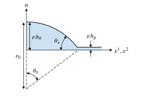
Figure 2: Radial cross-section of a spherical cap initial condition (scaled by $L$) with dimensionless radius of curvature $r_{0}$, maximum height $h_{0}$, and precursor film of thickness $h_{\text{p}}$.

3.3 Implementation using COMSOL Multiphysics and MATLAB

Throughout section 4, equations (33) and (40) are solved using the finite-element Coefficient Form PDE Interface in COMSOL Multiphysics 5.6 with LiveLink for MATLAB R2021b. In order to implement (33) and (40), we introduce the variable $\varGamma=N_{\text{surf}}\kappa^{*}+\varPi$ and express the problem as a system of second-order PDEs in $h$ and $\varGamma$. The system of PDEs is then solved by pre-computing the coefficients (including the components of the total body force, curvature tensor, and modified Levi–Civita tensor) over the solution mesh in MATLAB, then using COMSOL Multiphysics with all default settings and a solver tolerance of $10^{-5}$ (to ensure that the tolerance is less than $\varepsilon^{2}$ for the chosen value of $\varepsilon=4\times 10^{-3}$) to solve for the evolution of $h$ and $\varGamma$ over time. For the example simulations, we use a $200\times 200$ cell square mesh with linear Lagrange elements over a domain of $(x^{1},x^{2})\in[-1,1]\times[-1,1]$. Additionally, we choose zero-flux conditions on the boundaries of the computational domain. This does not affect the spreading of the initial droplet as we do not allow any simulations to run sufficiently long for the droplet to reach the edge of the domain.

4 Results

4.1 Effects of the Coriolis force in spin coating on a flat substrate

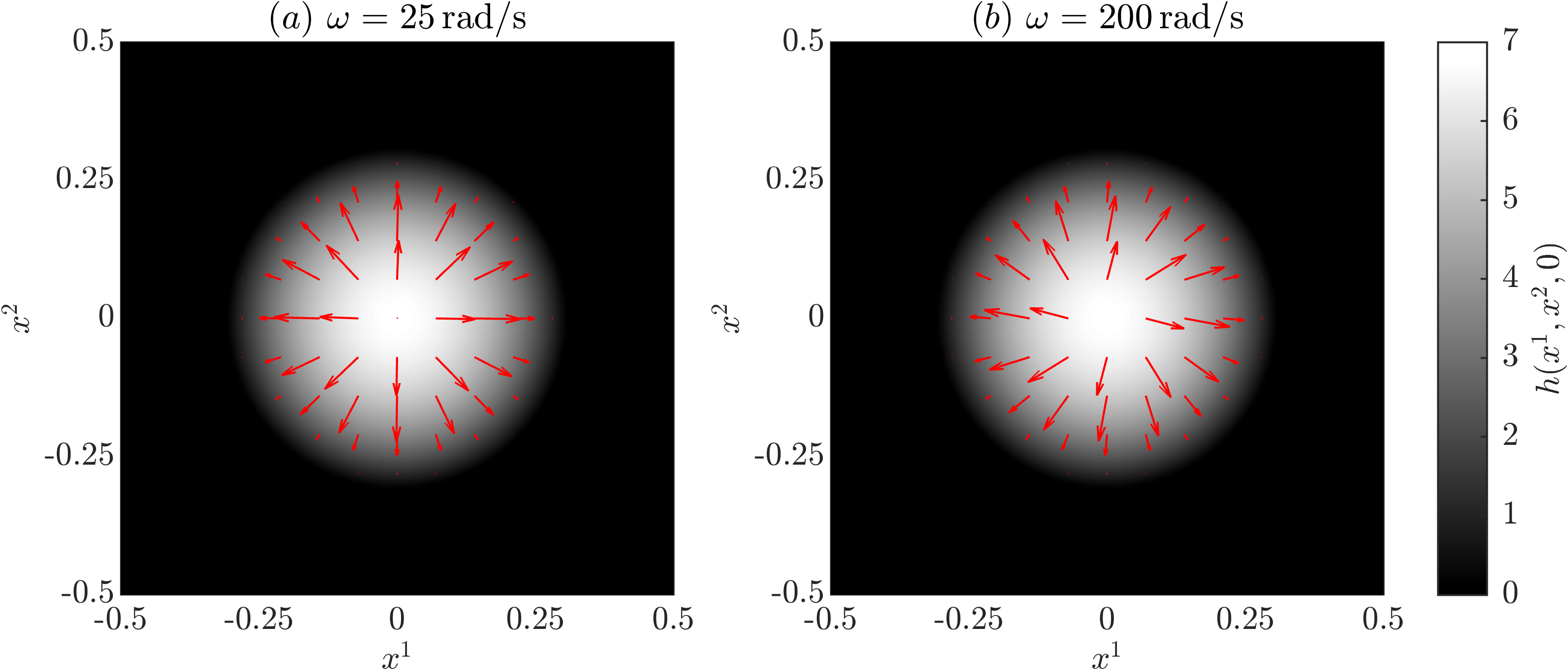
Figure 3: Vector field of the initial dimensionless volume flux, $\boldsymbol{q}(x^{1},x^{2},0)$, and colourmap of initial dimensionless film thickness, $h(x^{1},x^{2},0)$, for (a) transitional flow ($\omega=25\,\text{rad/s}$, $\mathit{Ta}=0.25$) and (b) centrifugal force-driven flow ($\omega=200\,\text{rad/s}$, $\mathit{Ta}=1.96$) on an anticlockwise-rotating substrate.

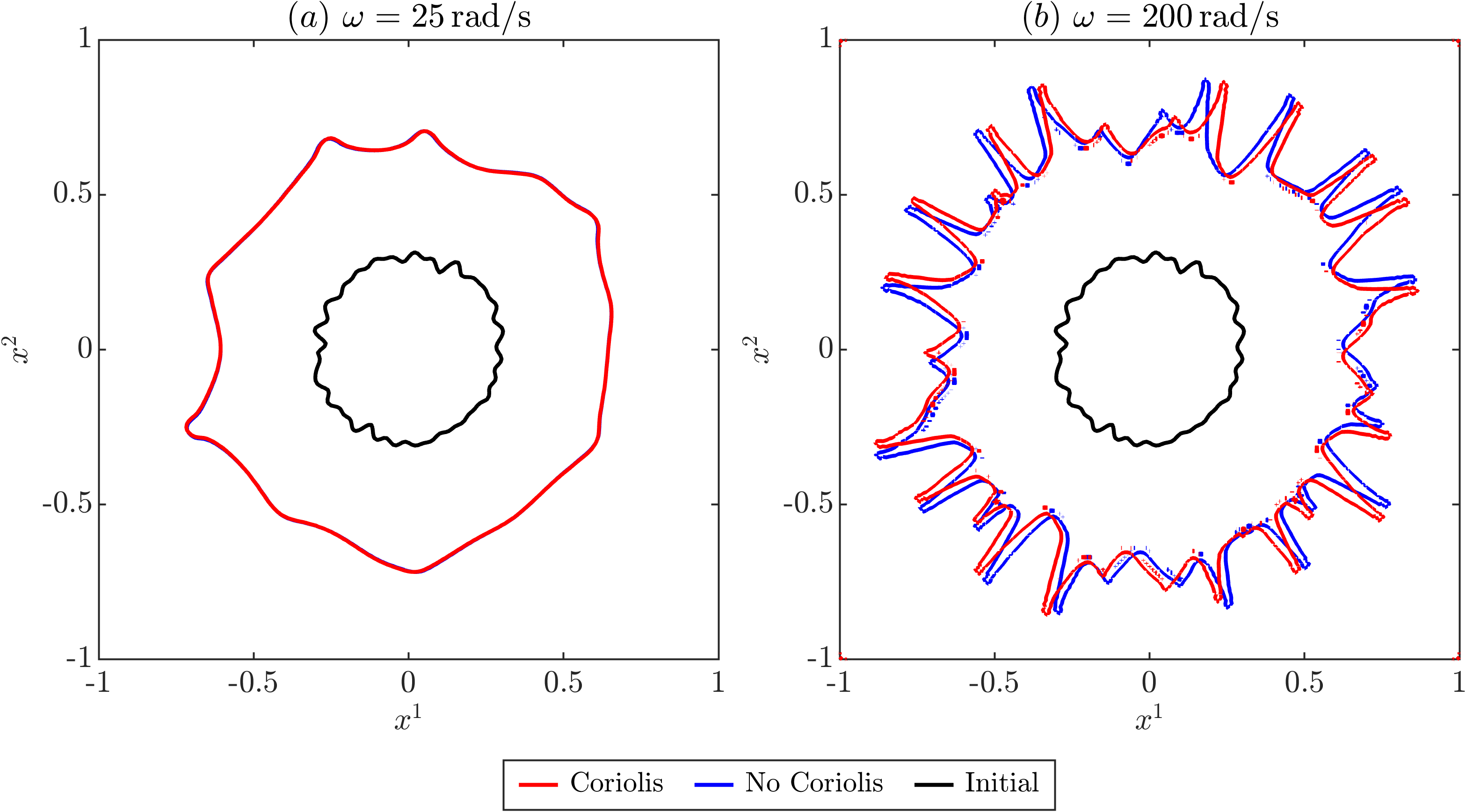
Figure 4: Contact line at $t=1.5$ with (red) and without (blue) the effects of the Coriolis force on a flat substrate from a randomly perturbed initial condition (black) on an anticlockwise-rotating substrate. (a) Transitional flow ($\omega=25\,\text{rad/s}$, $\mathit{Ta}=0.25$), showing the near-indistinguishable contact lines with and without the Coriolis force. (b) Centrifugal force-driven flow ($\omega=200\,\text{rad/s}$, $\mathit{Ta}=1.96$), demonstrating the deflection of radial fingers against the direction of substrate rotation due to the onset of the Coriolis force.

Before investigating the flow of spin-coated films on curved substrates, we will fist consider the base case of flow on a flat substrate with particular attention to the effect of the Coriolis force for the physical parameters considered here, which has not been included in previous models for flows on curved substrates (e.g. Weidner (2018); Duruk et al. (2023)). Figure 3 shows the instantaneous initial volume flux in a spherical droplet (47) on a rotating flat substrate (given in dimensionless Cartesian coordinates by $\boldsymbol{s}(x^{1},x^{2})=[x^{1},x^{2},0]$) in two different flow regimes: transitional flow at low angular velocity ($\omega=25\,\text{rad/s}$, $\mathit{Ta}=0.25$), where gravitational and centrifugal forces have a comparable effect; and centrifugal force-driven flow at high angular velocity ($\omega=200\,\text{rad/s}$, $\mathit{Ta}=1.96$). In the transitional regime (figure 3a), the volume flux is entirely in the radial direction. In the centrifugal force-driven regime (figure 3b), however, the volume flux is deflected in the clockwise direction due to the onset of the Coriolis force, against the anti-clockwise direction of substrate rotation. Compared to gravity and the leading-order component of centrifugal force, which do not scale with film thickness, the Coriolis force scales with $h^{2}$ (as seen in (40) and detailed in the derivation in appendix A). The effect will therefore be the strongest during the earliest stages of the spin coating process (as seen in the instantaneous initial volume flux), and diminish as the droplet spreads and thins. Figure 4 shows the contact line at $t=1.5$ with and without the effect of the Coriolis force (by setting $\mathit{Ta}=0$) for the spreading of a perturbed spherical droplet (48) on a flat substrate in transitional and centrifugal force-driven regimes. Here, we plot the contact line as the contour where $h=5h_{\text{p}}=0.5$, noting that the dimensionless film thickness in the wetted area remains above 0.8 even at the end of our simulations. Again, we see that at low angular velocity there is no appreciable difference in the contact line due to the Coriolis force. With increasing angular velocity, the introduction of the Coriolis force leads to a slight deflection of the fingering at the contact line against the direction of substrate rotation with no change in the wavelength or amplitude of the fingering instability.

In the case of centrifugal-force dominated flow, where $f_{\text{c}}\approx\omega^{2}L$ (and recalling the choice of characteristic velocity from (26)), the Reynolds number may be expressed as

$$\mathit{Re}=\frac{\rho u_{\text{c}}h_{\text{c}}}{\mu}\approx\varepsilon\bigg{(}\frac{\omega\rho Lh_{\text{c}}}{\mu}\bigg{)}^{2}=\varepsilon\mathit{Ta}^{2}.$$ (49)

This sets an upper bound of $\mathit{Ta}\lesssim 1$ in order to ensure that $\mathit{Re}\lesssim\varepsilon$, which limits the higher-order terms in (40) to at most $O(\varepsilon^{2})$. There is therefore a narrow range of angular velocities around $\mathit{Ta}\sim 1$ where the Coriolis force has an observable effect on the flow (such as in figures 3b and 4b), but where inertial effects can still be ignored. For the model and parameters considered here, we can conclude that while it is important to include the Coriolis force in order to accurately model the film dynamics, its effect is small enough that it is not likely to have a significant impact in practical applications.

4.2 Spin coating on non-axisymmetric curved substrates

We now consider the flow of a spin-coated film on two different non-axisymmetric curved substrates. In sections 4.2.1 and 4.2.2, we will discuss example simulations of a perturbed spherical droplet spreading on rotating parabolic cylinder- and saddle-shaped substrates, respectively. In each case, the results from additional realisations of the randomly-perturbed initial condition are reported in appendix C.

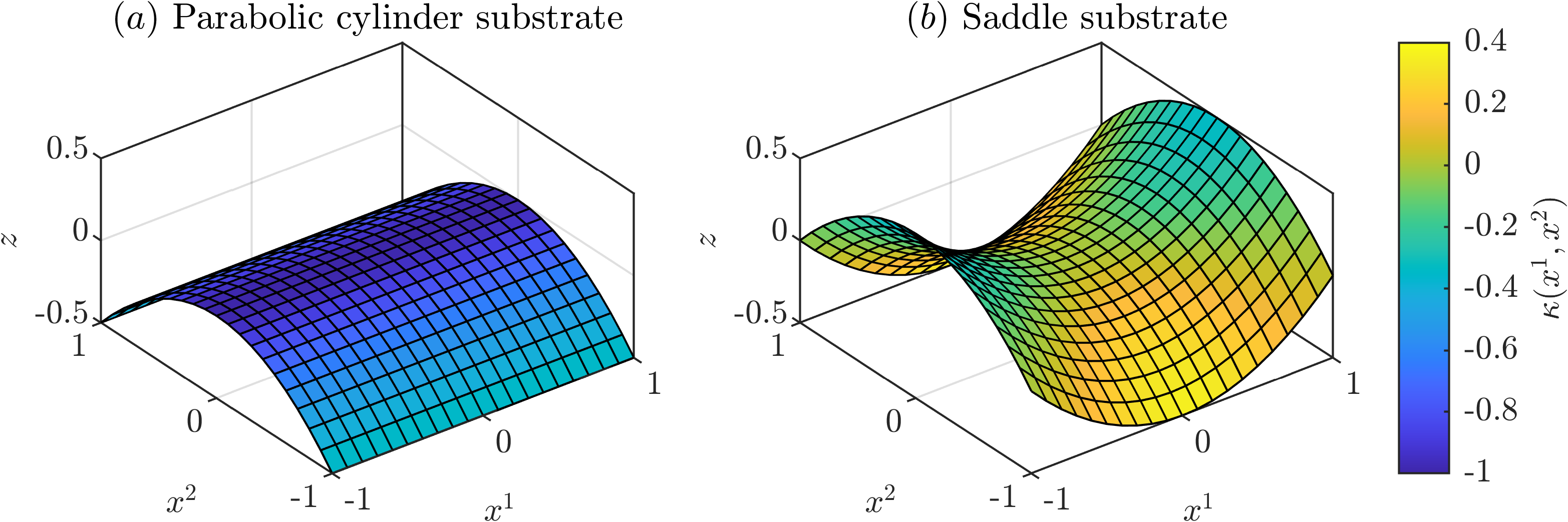
Figure 5: (a) Parabolic cylinder substrate (50) and (b) saddle substrate (51) in dimensionless Cartesian coordinates, coloured by the dimensionless substrate mean curvature, $\kappa(x^{1},x^{2})$.

4.2.1 Parabolic cylinder substrate

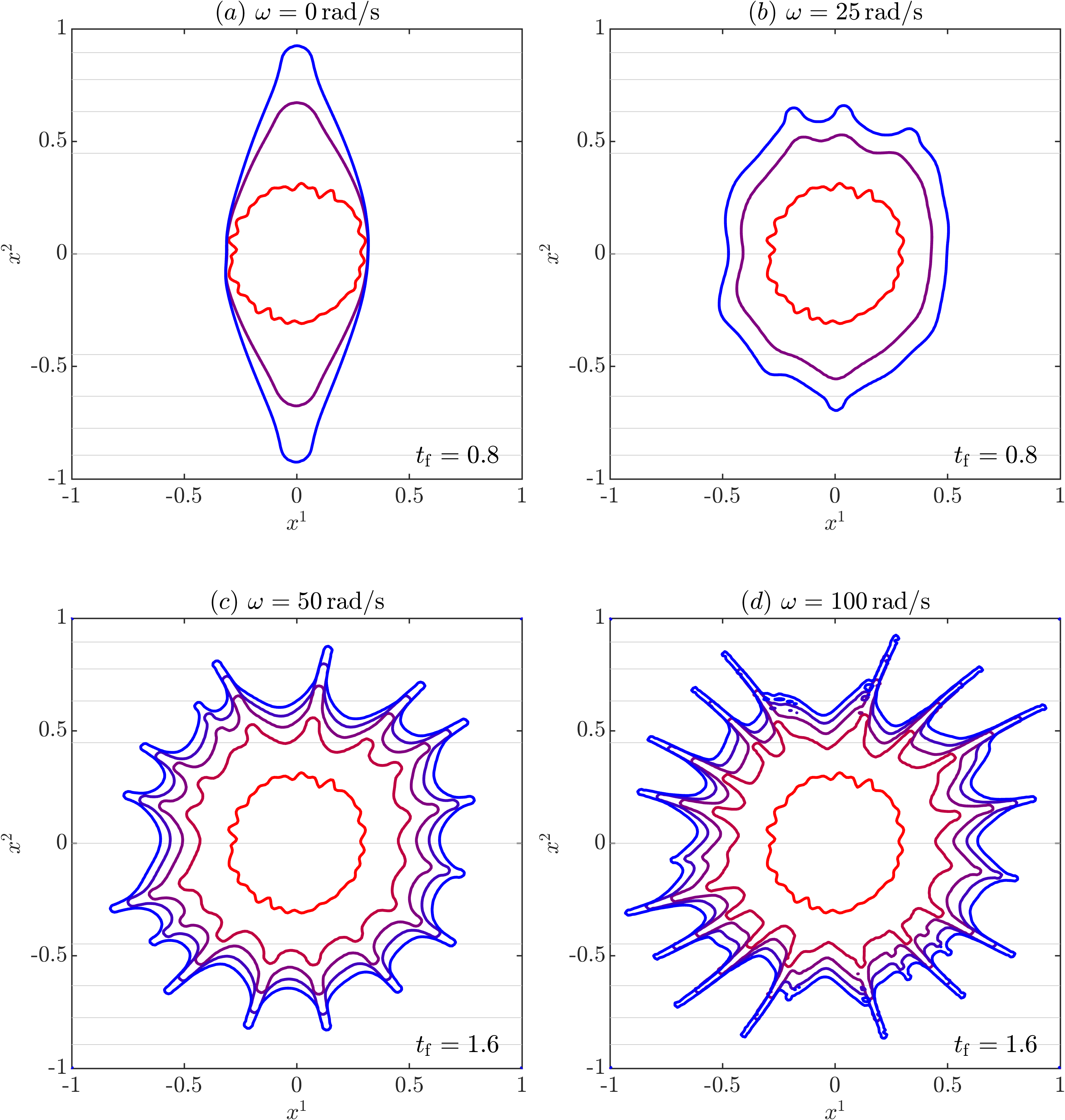
Figure 6: Evolution of the contact line on a parabolic cylinder substrate (equation (50) and figure 5a) from a randomly perturbed initial condition in intervals of $\Delta t=0.4$, coloured from red to blue with increasing $t$ up to $t_{\text{f}}$ on an anticlockwise-rotating substrate. Substrate contours with vertical spacing $\Delta z=0.1$ are shown in grey. (a) Contact line up to $t_{\text{f}}=0.8$ on a stationary substrate. (b) Contact line up to $t_{\text{f}}=1$ with $\omega=25\,\text{rad/s}$. (c) Contact line up to $t_{\text{f}}=1.6$ with $\omega=50\,\text{rad/s}$. (d) Contact line up to $t_{\text{f}}=1.6$ with $\omega=100\,\text{rad/s}$.

Figure 6 shows the evolution of the contact line of a perturbed spherical droplet (48) on a rotating parabolic cylinder substrate for angular velocities from $\omega=0\,\text{rad/s}$ to $100\,\text{rad/s}$. The substrate is described in dimensionless Cartesian coordinates by

$$\boldsymbol{s}(x^{1},x^{2})=\bigg{[}x^{1},x^{2},-\frac{(x^{2})^{2}}{2}\bigg{]},$$ (50)

and shown in figure 5a. In the gravity-driven regime on a stationary substrate ($\omega=0\,\text{rad/s}$, figure 6a), the initial droplet forms rivulets flowing down either side of the substrate in the direction of $\pm x^{2}$. As the angular velocity of the substrate is increased, the film dynamics enter a transitional regime, where there are competing effects from gravitational and centrifugal forces. At $\omega=25\,\text{rad/s}$ (figure 6b), the droplet begins to spread radially in all directions due to centrifugal force, but still with a preference toward the $\pm x^{2}$ directions and forming rivulets down either side of the substrate due to gravity. As the angular velocity is increased further, the dynamics become driven primarily by centrifugal force. At $\omega=50\,\text{rad/s}$ and $100\,\text{rad/s}$ (figures 6c and 6d), there is weak gravitational influence and the droplet spreads evenly in all directions. In this regime, the spreading droplet develops a fingering instability at the contact line similarly to on a flat substrate, with the growth rate of the fingers increasing with increasing angular velocity. At the leading order, the volume flux over the substrate surface (40) is driven by the component of the total body force tangent to the substrate surface. In the centrifugal force-driven regime, the tangential component of the total body force is greatest along the ridge of the substrate. At high angular velocity ($\omega=100\,\text{rad/s}$, figure 6d), this leads to a deflection of fingers in the $\pm x^{1}$ directions.

4.2.2 Saddle substrate

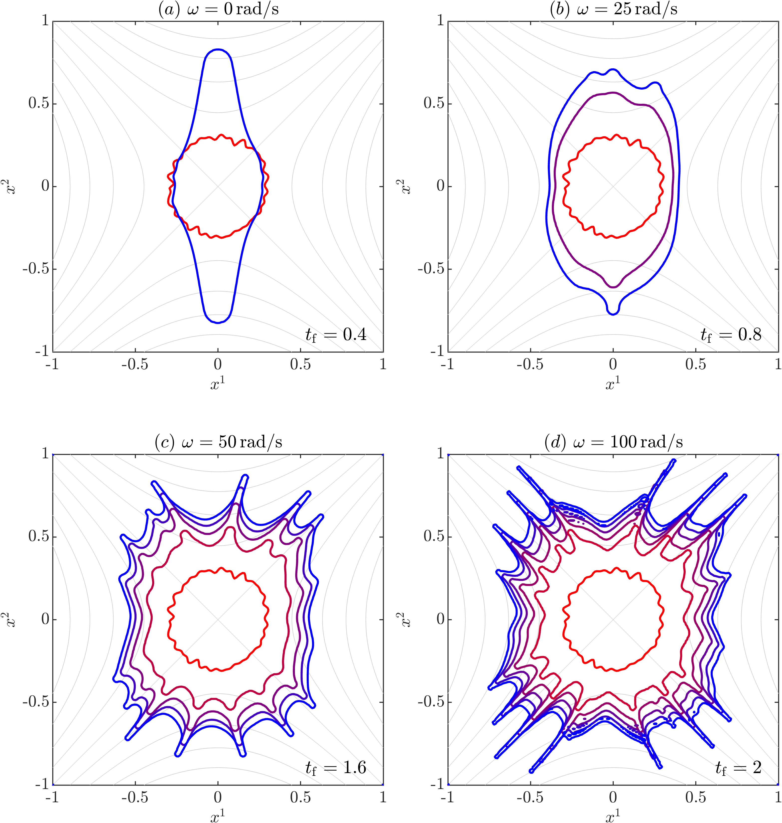
Figure 7: Evolution of the contact line on a saddle substrate (equation (51) and figure 5b) from a randomly perturbed initial condition in intervals of $\Delta t=0.4$, coloured from red to blue with increasing $t$ up to $t_{\text{f}}$ on an anticlockwise-rotating substrate. Substrate contours with vertical spacing $\Delta z=0.1$ are shown in grey. (a) Contact line up to $t_{\text{f}}=0.4$ on a stationary substrate. (b) Contact line up to $t_{\text{f}}=1$ with $\omega=25\,\text{rad/s}$. (c) Contact line up to $t_{\text{f}}=1.6$ with $\omega=50\,\text{rad/s}$. (d) Contact line up to $t_{\text{f}}=2$ with $\omega=100\,\text{rad/s}$.

Figure 7 shows the evolution of the contact line of a perturbed spherical droplet (48) on a rotating saddle substrate for angular velocities from $\omega=0\,\text{rad/s}$ to $100\,\text{rad/s}$. The substrate is described in dimensionless Cartesian coordinates by

$$\boldsymbol{s}(x^{1},x^{2})=\bigg{[}x^{1},x^{2},\frac{(x^{1})^{2}}{2}-\frac{(x^{2})^{2}}{2}\bigg{]},$$ (51)

and shown in figure 5b. Similarly to the parabolic cylinder, in the gravity-driven regime ($\omega=0\,\text{rad/s}$, figure 7a), the initial droplet forms rivulets along the downward-sloping $\pm x^{2}$ directions. At $\omega=25\,\text{rad/s}$ (figure 7b), the droplet again begins to spread radially in all directions, while still forming rivulets in the downward-sloping directions. On a saddle substrate, however, the centrifugal force is not strong enough to overcome the upward slope of the substrate in the $\pm x^{1}$ directions, leading to a more pronounced elliptically-shaped contact line. At high angular velocities, the film dynamics on a saddle substrate begin to differ significantly from those on the parabolic cylinder. In particular, for centrifugal force-driven flow on a saddle substrate, the tangential component of the total body force is greatest on the diagonals $x^{1}=\pm x^{2}$, along which the substrate is horizontal. As with the parabolic cylinder substrate, we continue to observe that the thickness of the film behind the moving front is the same as on a flat substrate at high angular velocity ($\omega=100\,\text{rad/s}$). At $\omega=50\,\text{rad/s}$ and $100\,\text{rad/s}$ (figures 6c and 6d), the spreading droplet again develops a fingering instability at the contact line. In this case, however, the fingering does not develop in all directions, and grows in an ‘X’-shape, primarily along the diagonal $z=0$ contours ($x^{1}=\pm x^{2}$) in the direction of the greatest tangential body force.

4.3 Film thickness and surface coverage

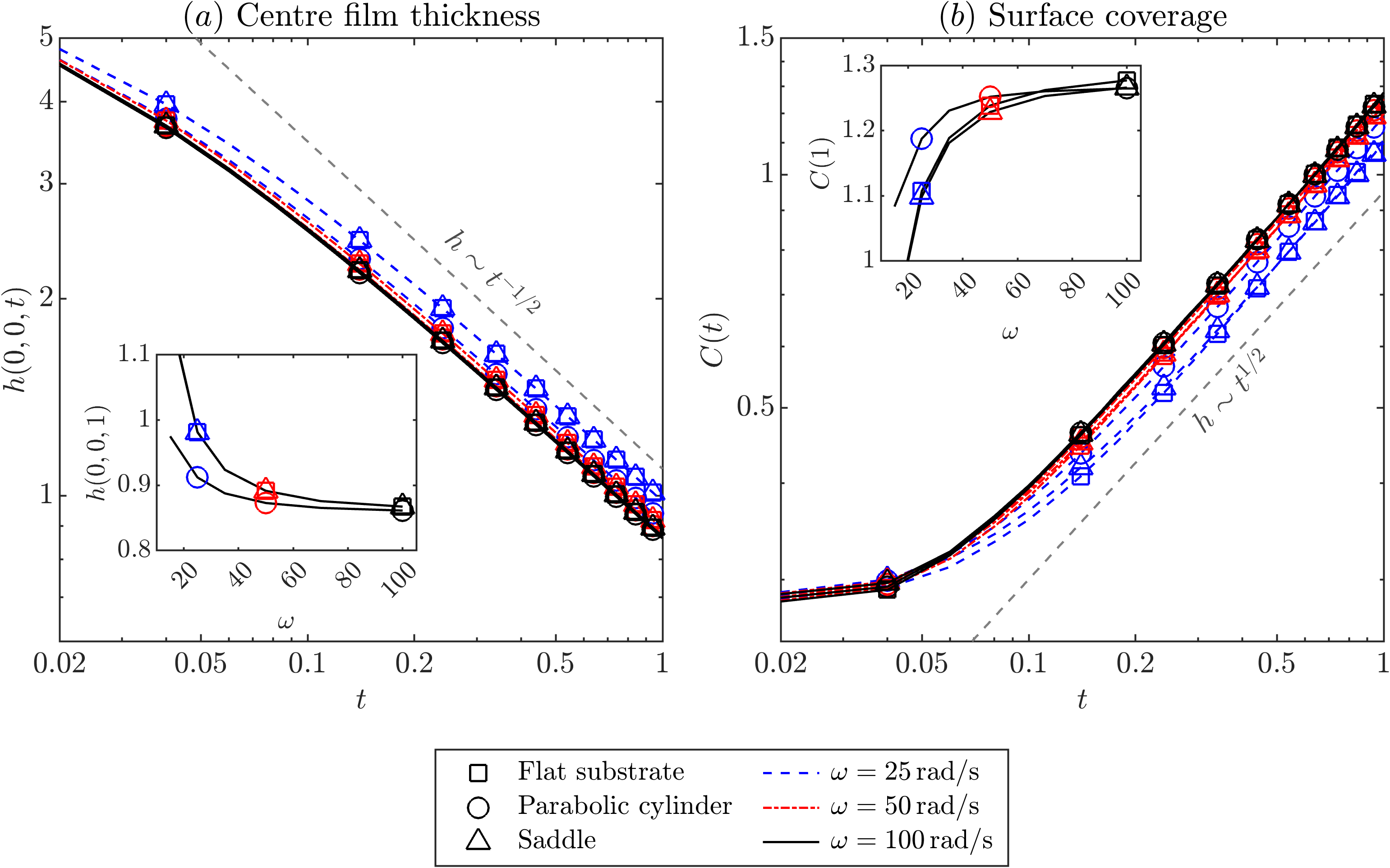
Figure 8: Temporal evolution of $(a)$ the film thickness at the substrate centre, $h(0,0,t)$, and $(b)$ the surface area of the fluid-covered region, $C(t)$, on flat, parabolic cylinder and saddle substrates for angular velocities $\omega=25\,\text{rad/s}$, $50\,\text{rad/s}$ and $100\,\text{rad/s}$. In each case, the inset shows the film thickness or surface coverage at $t=1$ as a function of the substrate angular velocity, $\omega$. The lines between markers in the inset plots include results for intermediate angular velocities not shown in the main plot.

To quantify the film evolution, we report in figure 8a the film thickness at the substrate centre, $h(0,0,t)$, on the three considered substrates (flat, parabolic cylinder and saddle), for several values of the angular velocity. On all substrates and for all angular velocities, the centre film thickness decreases as $h\sim t^{-1/2}$ from $t\approx 0.1$ onwards, and the variations due to the substrate and angular velocity are small compared to the overall variation over time. Furthermore, at a high angular velocity ($\omega=100\,\text{rad/s}$), the centre film thickness remains the same as on a flat substrate while the droplet spreads. The same power law for film thickness evolution on cylindrical and spherical substrates without rotation (Takagi & Huppert, 2010) and flat substrates with rotation (Melo et al., 1989) was measured experimentally and predicted analytically by self-similar solutions derived from the lubrication equation with surface tension and hydrostatic pressure neglected away from the contact line.

We also define, and report in figure 8b, the surface coverage at time $t$ as the substrate surface area within the wetted region,

$$C(t)=\iint_{\Omega}\phi(x,^{1},x^{2},t)\sqrt{G(x^{1},x^{2})}\,\mathrm{d}x^{1}\mathrm{d}x^{2},$$ (52)

where $\Omega=[-1,1]\times[-1,1]$ is the domain and

$$\phi(x,^{1},x^{2},t)=\begin{cases}1&\text{if }h(x^{1},x^{2},t)\geq 5h_{\text{p}},\\ 0&\text{otherwise.}\end{cases}$$ (53)

Here, we again choose $h\geq 5h_{\text{p}}$ as the threshold for the wetted area to be consistent with the contact lines plotted in sections 4.1 and 4.2.

As expected, larger angular velocities lead to faster initial film thinning and, therefore, to thinner films and larger surface coverage at later times, scaling as $C\sim t^{1/2}$. At smaller angular velocities (gravity-driven flows), thinner films are obtained on the parabolic cylinder substrate than on the flat and saddle substrates, which may be ascribed to the larger substrate curvature at the centre. At larger angular velocities (centrifugal force-driven flows), however, the substrate geometry does not significantly affect the overall rate of dispersal over the surface. The key difference in the results between different geometries is the shape of the droplet: although the film spreads a similar amount, its distribution is no longer axisymmetric on the parabolic cylinder and saddle substrates.

5 Conclusions

In this work, we have derived and implemented a model for the evolution of a thin fluid film on a rotating curved substrate surface, allowing for an arbitrary substrate parameterisation, and including the effects of surface tension, disjoining pressure, gravity, centrifugal, and Coriolis forces. We can consider this either as an extension of existing models of spin coating (such as Schwartz & Roy (2004) and Weidner (2018)) to allow for more complex and non-axisymmetric substrate geometry, or as an extension of models for thin film flow over stationary curved substrates (such as Roy et al. (2002), Thiffeault & Kamhawi (2006), and Mayo et al. (2015)) to include centrifugal and Coriolis forces due to substrate rotation. We implemented our generalised model using COMSOL Multiphysics and MATLAB to simulate the evolution of spin-coated films on flat and curved substrates at a range of angular velocities.

On a flat substrate, we demonstrated that the Coriolis force has a negligible effect at low substrate angular velocity, and at high angular velocity leads to a slight deflection of the flow against the direction of substrate rotation. This deflection was observed in both the instantaneous initial volume flux at the start of spin coating, and in the fingering instability at the contact line as the spin-coated droplet spreads. Our analysis agrees with the conclusions from Myers & Charpin (2001), showing that while the Coriolis force has only a small effect, there is a range of parameters (when $\mathit{Ta}\sim 1$) where the Coriolis force cannot be neglected, but where inertial effects can still be ignored.

On parabolic cylinder and saddle substrate geometries, we showed example simulations of spin coating at a range of angular velocities to demonstrate the transition from gravity-driven to centrifugal force-driven flow. In both cases, as the angular velocity is increased, a droplet initially at the centre of the substrate shifted from draining in the downward-sloping directions to spreading in the directions where the tangential component of the centrifugal force is greatest. On a parabolic cylinder substrate at $\omega=100\,\text{rad/s}$, this leads to a similar pattern of fingering at the contact line to a flat substrate, however with the fingers deflected along the direction of the ridge (the $\pm x^{1}$ directions). On a saddle substrate at $\omega=100\,\text{rad/s}$, the effect of substrate geometry was clearer, with the fingers at the contact line growing in an ‘X’-shape (along the $x^{1}=\pm x^{2}$ diagonals). Furthermore, we showed that for both parabolic cylinder and saddle substrates, the film thickness at the substrate centre and the wetted area remain similar over time to those for a droplet spreading on a flat substrate, demonstrating that the key difference between substrate geometries is the shape of the spreading droplet and the direction of fingering.

There are several natural ways in which the present work could be extended. In particular, in order to investigate higher angular velocities where the Coriolis force would have a stronger effect (where $\mathit{Ta}>1$, and hence $\mathit{Re}>\varepsilon$), however, a model incorporating inertial effects would be required. Additionally, a stability analysis around the contact line on a curved substrate with both gravitational and centrifugal forces may provide a more detailed explanation for the complex fingering patterns observed on a saddle substrate.

[Funding]This work is part of the project ”Development of a multi-axis spin-coating system to coat curved surfaces” funded by the New Zealand Ministry of Business, Innovation and Employment Endeavour fund (grant number UOCX1904). This funding is gratefully acknowledged.

[Declaration of interests]The authors report no conflict of interest.

[Author ORCIDs]Ross G. Shepherd, https://orcid.org/0000-0003-3489-018X; Edouard Boujo, https://orcid.org/0000-0002-4448-6140; Mathieu Sellier, https://orcid.org/0000-0002-5060-1707

Appendix A Integration of the Navier–Stokes equations normal to the substrate

In order to integrate the simplified NS equations (32) in the direction normal to the substrate, we introduce an perturbation expansion in $\varepsilon$ for the velocity, pressure, and body force as follows, and omit the tildes over dimensionless variables for brevity:

$$\left.\begin{array}[]{ccccccl}u^{\alpha}&=&u^{\alpha}_{(0)}&+&\varepsilon u^{\alpha}_{(1)}&+&O(\varepsilon^{2}),\\[4.0pt] p&=&p_{(0)}&+&\varepsilon p_{(1)}&+&O(\varepsilon^{2}),\\[4.0pt] f^{\alpha}&=&f^{\alpha}_{(0)}&+&\varepsilon f^{\alpha}_{(1)}&+&O(\varepsilon^{2}),\\[4.0pt] f^{n}&=&f^{n}_{(0)}&+&O(\varepsilon).\end{array}\quad\right\}$$ (54)

Substituting (22) for $\boldsymbol{e}^{+\alpha}$, the $O(1)$ and $O(\varepsilon)$ parts of the tangential body force can be written as

$$f^{\alpha}_{(0)}=\big{[}N_{\text{grav}}\hat{\boldsymbol{g}}-N_{\text{cent}}\hat{\boldsymbol{\omega}}\times\big{(}\hat{\boldsymbol{\omega}}\times\boldsymbol{s})\big{]}\boldsymbol{\cdot}\boldsymbol{e}^{\alpha},$$ (55)

$$f^{\alpha}_{(1)}=-\big{[}nN_{\text{cent}}\hat{\boldsymbol{\omega}}\times(\hat{\boldsymbol{\omega}}\times\hat{\boldsymbol{n}})+2\mathit{Ta}\hat{\boldsymbol{\omega}}\times\boldsymbol{u}_{(0)}\big{]}\boldsymbol{\cdot}\boldsymbol{e}^{\alpha}+nK_{\beta}{}^{\alpha}f^{\beta}_{(0)},$$ (56)

where $\boldsymbol{u}_{(0)}=u^{\alpha}_{(0)}\boldsymbol{e}_{\alpha}$ is the leading-order velocity vector. Similarly, the leading-order normal body force is

$$f^{n}_{(0)}=\big{[}N_{\text{grav}}\hat{\boldsymbol{g}}-N_{\text{cent}}\hat{\boldsymbol{\omega}}\times\big{(}\hat{\boldsymbol{\omega}}\times\boldsymbol{s})\big{]}\boldsymbol{\cdot}\hat{\boldsymbol{n}}.$$ (57)

Here, we see that the $O(1)$ body force terms are constant in $n$, but the $O(\varepsilon)$ terms depend on $n$ both explicitly and implicitly due to variation in $\boldsymbol{u}_{(0)}$ in the normal direction.

Substituting the perturbation expansion (54), together with (22) for $G^{+\alpha\beta}$, the lubrication equations (32) at $O(1)$ and $O(\varepsilon)$ are

$$\left.\begin{array}[]{c}\displaystyle{-\frac{\partial p_{(0)}}{\partial n}=0,}\\[8.0pt] \displaystyle{-\nabla^{\alpha}p_{(0)}+\frac{\partial^{2}u^{\alpha}_{(0)}}{\partial n^{2}}+f^{\alpha}_{(0)}=0,}\end{array}\quad\right\}$$ (58)

$$\left.\begin{array}[]{c}\displaystyle{-\frac{\partial p_{(1)}}{\partial n}+f^{n}_{(0)}=0,}\\[8.0pt] \displaystyle{-\nabla^{\alpha}p_{(1)}-2nK_{\beta}{}^{\alpha}\nabla^{\beta}p_{(0)}+\frac{\partial^{2}u^{\alpha}_{(1)}}{\partial n^{2}}-\big{(}\kappa\delta_{\beta}{}^{\alpha}+2K_{\beta}{}^{\alpha}\big{)}\frac{\partial u^{\beta}_{(0)}}{\partial n}+f^{\alpha}_{(1)}=0,}\end{array}\quad\right\}$$ (59)

where $\nabla^{\alpha}=G^{\alpha\beta}\partial/\partial x^{\beta}$ is a contravariant component of the substrate gradient. The corresponding perturbation expansions of the dimensionless boundary conditions are ${u^{\alpha}_{(0)}=u^{\alpha}_{(1)}=0}$ on $n=0$, and

$$\left.\begin{array}[]{cc}p_{(0)}=-N_{\text{surf}}\kappa-\varPi,&p_{(1)}=-N_{\text{surf}}(\kappa_{2}h+\Delta_{S}h),\\[4.0pt] \displaystyle\frac{\partial u^{\alpha}_{(0)}}{\partial n}=0,&\displaystyle\frac{\partial u^{\alpha}_{(1)}}{\partial n}=0,\end{array}\quad\right\}\quad\text{on }n=h.$$ (60)

Integrating (58) with respect to $n$ with boundary conditions (60) gives the standard leading-order lubrication model:

$$p_{(0)}=-N_{\text{surf}}\kappa-\varPi,\qquad u^{\alpha}_{(0)}=\bigg{(}hn-\frac{n^{2}}{2}\bigg{)}\bigg{(}\nabla^{\alpha}(N_{\text{surf}}\kappa+\varPi)+f^{\alpha}_{(0)}\bigg{)},$$ (61)

which is equivalent to equation (34) from Roy et al. (2002) and equation (IV.7) from Thiffeault & Kamhawi (2006).

Let $\omega^{\alpha}=\hat{\boldsymbol{\omega}}\boldsymbol{\cdot}\boldsymbol{e}^{\alpha}$ and $\omega^{n}=\hat{\boldsymbol{\omega}}\boldsymbol{\cdot}\hat{\boldsymbol{n}}$ be the tangential and normal components of $\hat{\boldsymbol{\omega}}$ in the substrate coordinate system, and let $\epsilon_{\beta}{}^{\alpha}$ be a mixed component of the modified Levi–Civita tensor, $\mathsfbi{E}=\epsilon_{\alpha\beta}\boldsymbol{e}^{\alpha}\boldsymbol{e}^{\beta}$, defined by

$$\epsilon_{\alpha\beta}=(\boldsymbol{e}_{\alpha}\times\boldsymbol{e}_{\beta})\boldsymbol{\cdot}\hat{\boldsymbol{n}}=\big{\lVert}\boldsymbol{e}_{1}\times\boldsymbol{e}_{2}\big{\rVert}\begin{cases}1&\text{if }\alpha=1,\,\beta=2,\\ -1&\text{if }\alpha=2,\,\beta=1,\\ 0&\text{otherwise.}\end{cases}$$ (62)

This allows the Coriolis force term in (56) to be written as

$$(\hat{\boldsymbol{\omega}}\times\boldsymbol{u}_{(0)})\boldsymbol{\cdot}\boldsymbol{e}^{\alpha}=\omega^{n}\epsilon_{\beta}{}^{\alpha}\bigg{(}hn-\frac{n^{2}}{2}\bigg{)}\bigg{(}\nabla^{\beta}(N_{\text{surf}}\kappa+\varPi)+f^{\beta}_{(0)}\bigg{)}.$$ (63)

The $O(\varepsilon)$ tangential body force can then be expressed explicitly in terms of $n$:

$$\begin{split}f^{\alpha}_{(1)}=&\;nN_{\text{cent}}(\hat{\boldsymbol{\omega}}\times(\hat{\boldsymbol{\omega}}\times\hat{\boldsymbol{n}}))\boldsymbol{\cdot}\boldsymbol{e}^{\alpha}+nK_{\beta}{}^{\alpha}f^{\beta}_{(0)}\\ &-2\mathit{Ta}\omega^{n}\epsilon_{\beta}{}^{\alpha}\bigg{(}hn-\frac{n^{2}}{2}\bigg{)}\bigg{(}\nabla^{\beta}(N_{\text{surf}}\kappa+\varPi)+f^{\beta}_{(0)}\bigg{)}.\end{split}$$ (64)

Integrating the pressure equation from (59) in $n$ with the boundary condition (60) gives

$$p_{(1)}=-N_{\text{surf}}(\kappa_{2}h+\Delta_{S}h)-f^{n}_{(0)}(h-n).$$ (65)

Now substituting (64) and (65) and collecting like terms, we can re-write (59) as

$$A^{\alpha}+nB^{\alpha}+n^{2}C^{\alpha}+\frac{\partial^{2}u^{\alpha}_{(1)}}{\partial n^{2}}=0,$$ (66)

where

$$\left.\begin{array}[]{rl}A^{\alpha}=&\;N_{\text{surf}}\nabla^{\alpha}(k_{2}h+\Delta_{S}h)+\nabla^{\alpha}\big{(}hf^{n}_{(0)}\big{)}\\[4.0pt] &-\;h\big{(}\kappa\delta_{\beta}{}^{\alpha}+2K_{\beta}{}^{\alpha}\big{)}\big{(}\nabla^{\beta}(N_{\text{surf}}\kappa+\varPi)+f^{\beta}_{(0)}\big{)},\\[8.0pt] B^{\alpha}=&-\;\nabla^{\alpha}f^{n}_{(0)}+\;N_{\text{cent}}(\hat{\boldsymbol{\omega}}\times(\hat{\boldsymbol{\omega}}\times\hat{\boldsymbol{n}}))\boldsymbol{\cdot}\boldsymbol{e}^{\alpha}\\[4.0pt] &+\;\big{(}\kappa\delta_{\beta}{}^{\alpha}+4K_{\beta}{}^{\alpha}-2\mathit{Ta}h\omega^{n}\epsilon_{\beta}{}^{\alpha}\big{)}\nabla^{\beta}(N_{\text{surf}}\kappa+\varPi)\\[4.0pt] &+\;\big{(}\kappa\delta_{\beta}{}^{\alpha}+3K_{\beta}{}^{\alpha}-2\mathit{Ta}h\omega^{n}\epsilon_{\beta}{}^{\alpha}\big{)}f^{\beta}_{(0)},\\[8.0pt] C^{\alpha}=&2\mathit{Ta}\omega^{n}\epsilon_{\beta}{}^{\alpha}\big{(}\nabla^{\beta}(N_{\text{surf}}\kappa+\varPi)+f^{\beta}_{(0)}\big{)}.\end{array}\quad\right\}$$ (67)

Integrating (66) with boundary conditions (60), the $O(\varepsilon)$ velocity is

$$u^{\alpha}_{(1)}=A^{\alpha}\bigg{(}hn-\frac{n^{2}}{2}\bigg{)}+B^{\alpha}\bigg{(}\frac{h^{2}n}{2}-\frac{n^{3}}{6}\bigg{)}+C^{\alpha}\bigg{(}\frac{h^{3}n}{3}-\frac{n^{4}}{12}\bigg{)}.$$ (68)

Similar to (54), we introduce a perturbation expansion for the dimensionless volume flux over the substrate surface:

$$q^{\alpha}=q^{\alpha}_{(0)}+\varepsilon q^{\alpha}_{(1)}+O(\varepsilon^{2}).$$ (69)

Substituting (54) into (28), the $O(1)$ and $O(\varepsilon)$ terms of the flux are

$$q^{\alpha}_{(0)}=\int_{0}^{h}u^{\alpha}_{(0)}\,\mathrm{d}n,$$ (70)

$$q^{\alpha}_{(1)}=\int_{0}^{h}\big{(}u^{\alpha}_{(1)}-\kappa nu^{\alpha}_{(0)}\big{)}\mathrm{d}n.$$ (71)

Integrating, the leading-order flux can be expressed as

$$q^{\alpha}_{(0)}=\frac{h^{3}}{3}\bigg{(}\nabla^{\alpha}(N_{\text{surf}}\kappa+\varPi)+f^{\alpha}_{(0)}\bigg{)},$$ (72)

and the $O(\varepsilon)$ flux as

$$q^{\alpha}_{(1)}=\frac{h^{3}}{3}A^{\alpha}+\frac{5h^{4}}{24}\bigg{[}B^{\alpha}-\kappa\bigg{(}\nabla^{\alpha}(N_{\text{surf}}\kappa+\varPi)+f^{\alpha}_{(0)}\bigg{)}\bigg{]}+\frac{3h^{5}}{20}C^{\alpha}.$$ (73)

Finally, substituting (67) and combining the $O(1)$ and $O(\varepsilon)$ terms, the components of the dimensionless volume flux over the substrate are

$$\begin{split}q^{\alpha}=\frac{h^{3}}{3}\bigg{[}&\bigg{(}\delta_{\beta}{}^{\alpha}-\varepsilon h\bigg{(}\kappa\delta_{\beta}{}^{\alpha}-\frac{1}{2}K_{\beta}{}^{\alpha}\bigg{)}-\varepsilon h^{2}\omega^{n}\frac{4\mathit{Ta}}{5}\epsilon_{\beta}{}^{\alpha}\bigg{)}\nabla^{\beta}(N_{\text{surf}}\kappa^{*}+\varPi)\\ &+\bigg{(}\delta_{\beta}{}^{\alpha}-\varepsilon h\bigg{(}\kappa\delta_{\beta}{}^{\alpha}+\frac{1}{2}K_{\beta}{}^{\alpha}\bigg{)}-\varepsilon h^{2}\omega^{n}\frac{4\mathit{Ta}}{5}\epsilon_{\beta}{}^{\alpha}\bigg{)}f^{\beta}_{(0)}\\ &+\varepsilon f^{n}_{(0)}\nabla^{\alpha}h+\varepsilon hN_{\text{cent}}(\hat{\boldsymbol{\omega}}\times(\hat{\boldsymbol{\omega}}\times\hat{\boldsymbol{n}}))\boldsymbol{\cdot}\boldsymbol{e}^{\alpha}\bigg{]}+O(\varepsilon\mathit{Re},\varepsilon^{2}).\end{split}$$ (74)

Appendix B Effect of precursor film thickness

\begin{overpic}[width=212.47617pt,trim=0.0pt 0.0pt 0.0pt 0.0pt,clip={true}]{contact_line_omega_100_Ta_98_hinf_0.075} \end{overpic} \begin{overpic}[width=212.47617pt,trim=0.0pt 0.0pt 0.0pt 0.0pt,clip={true}]{contact_line_omega_100_Ta_98_hinf_0.1} \end{overpic}

\begin{overpic}[width=212.47617pt,trim=0.0pt 0.0pt 0.0pt 0.0pt,clip={true}]{contact_line_omega_100_Ta_98_hinf_0.125} \end{overpic} \begin{overpic}[width=212.47617pt,trim=0.0pt 0.0pt 0.0pt 0.0pt,clip={true}]{contact_line_omega_100_Ta_98_hinf_0.15} \end{overpic}

Figure 9: Evolution of the contact line on a flat substrate from a randomly perturbed initial condition in intervals of $\Delta t=0.4$, coloured from red to blue with increasing $t$ up to $t_{\text{f}}=1.6$, on an anticlockwise-rotating substrate with $\omega=100\,\text{rad/s}$, for different values of the precursor film thickness: $(a)$ $h_{p}=0.075$, $(b)$ $h_{p}=0.1$, $(c)$ $h_{p}=0.125$, $(d)$ $h_{p}=0.15$.

Figure 9 shows the effect of the precursor film thickness on the evolution of the contact line on the flat substrate rotating at $\omega=100\,\text{rad/s}$. Differences are observed when $h_{p}\leq 0.075$, which are due to a numerical instability developing when the mesh is too coarse compared to the precursor film thickness. Conversely, the results are converged and robust for $h_{p}\geq 0.1$: while small localised differences can be observed, the overall spreading rate and shape are unaffected. In any case, the conclusions of the present study obtained with $h_{p}=0.1$ remain unchanged.

Appendix C Effect of the initial condition

\begin{overpic}[width=212.47617pt,trim=0.0pt 0.0pt 0.0pt 0.0pt,clip={true}]{cylinder_front_omega_100_Ta_98_N_1_10_t_1.6} \end{overpic} \begin{overpic}[width=212.47617pt,trim=0.0pt 0.0pt 0.0pt 0.0pt,clip={true}]{saddle_front_omega_100_Ta_98_N_1_10_t_1.6} \end{overpic}

Figure 10: Contact line at $t=1.6$ from randomly perturbed initial conditions on an anticlockwise-rotating $(a)$ parabolic cylinder substrate and $(b)$ saddle substrate with $\omega=100\,\text{rad/s}$. Thin coloured lines: 10 independent realisations. Thick black line: ensemble-averaged film. Substrate contours with vertical spacing $\Delta z=0.1$ are shown in grey.

Figure 10 shows the contact lines obtained at $t=1.6$ for 10 different realisations of the randomly perturbed initial condition (47–48) on parabolic cylinder and saddle substrates rotating at $\omega=100\,\text{rad/s}$. While the location of the fingers depends on the individual realisation, this confirms that the observations of section 4.2 are robust, that is, the fingers are consistently deflected in the $\pm x^{1}$ directions on the parabolic cylinder substrate and along the $x^{1}=\pm x^{2}$ diagonals on the saddle substrate.

We note in passing that for this specific value of the angular velocity, the ensemble-averaged contact line (shown with a thick black line) spreads non-axisymmetrically: on the parabolic cylinder substrate, the contact line moves approximately 10% faster in the $\pm x^{1}$ directions; on the saddle substrate, the contact line develops into a square shape.

References

- Balestra et al. (2016) Balestra, Gioele, Brun, P.-T. & Gallaire, François 2016 Rayleigh-Taylor instability under curved substrates: An optimal transient growth analysis. Physical Review Fluids 1 (8), 83902.
- Balestra et al. (2018) Balestra, Gioele, Nguyen, David Minh-Phuc & Gallaire, François 2018 Rayleigh-Taylor instability under a spherical substrate. Physical Review Fluids 3 (8), 84005.
- Chen et al. (2009) Chen, Long-jiang, Liang, Yi-yong, Luo, Jian-bo, Zhang, Chun-hui & Yang, Guo-guang 2009 Mathematical modeling and experimental study on photoresist whirl-coating in convex-surface laser lithography. Journal of Optics A: Pure and Applied Optics 11 (10), 105408.
- Cho et al. (2005) Cho, Hao-Chiang, Chou, Fu-Chu, Wang, Ming-Wen & Tsai, Chu-Shu 2005 Effect of Coriolis Force on Fingering Instability and Liquid Usage Reduction. Japanese Journal of Applied Physics 44 (19), L606–L609.
- Cohen & Lightfoot (2011) Cohen, Edward & Lightfoot, E. J. 2011 Coating Processes. In Kirk-Othmer Encyclopedia of Chemical Technology. Hoboken, NJ, USA: John Wiley & Sons, Inc.
- Duruk et al. (2021) Duruk, Selin, Boujo, Edouard & Sellier, Mathieu 2021 Thin Liquid Film Dynamics on a Spinning Spheroid. Fluids 6 (9).
- Duruk et al. (2023) Duruk, Selin, Shepherd, Ross G., Boujo, Edouard & Sellier, Mathieu 2023 Three-dimensional nonlinear dynamics of a thin liquid film on a spinning ellipsoid. Physics of Fluids 35 (7), 072115.
- Emslie et al. (1958) Emslie, Alfred G., Bonner, Francis T. & Peck, Leslie G. 1958 Flow of a Viscous Liquid on a Rotating Disk. Journal of Applied Physics 29 (5), 858–862.
- Evans et al. (2004) Evans, PL, Schwartz, LW & Roy, RV 2004 Steady and unsteady solutions for coating flow on a rotating horizontal cylinder: Two-dimensional theoretical and numerical modeling. Physics of Fluids 16 (8), 2742–2756.
- Fraysse & Homsy (1994) Fraysse, Nathalie & Homsy, George M. 1994 An experimental study of rivulet instabilities in centrifugal spin coating of viscous Newtonian and non-Newtonian fluids. Physics of Fluids 6 (4), 1491–1504.
- Howell (2003) Howell, P.D. 2003 Surface-tension-driven flow on a moving curved surface. Journal of Engineering Mathematics 45, 283–308.
- Kang et al. (2016) Kang, D., Nadim, A. & Chugunova, M. 2016 Dynamics and equilibria of thin viscous coating films on a rotating sphere. Journal of Fluid Mechanics 791, 495–518.
- Lebedev & Cloud (2003) Lebedev, Leonid P. & Cloud, Michael J. 2003 Tensor Analysis. World Scientific Publishing Company.
- Ledda et al. (2022) Ledda, Pier Giuseppe, Pezzulla, M., Jambon-Puillet, E., Brun, P.-T. & Gallaire, F. 2022 Gravity-driven coatings on curved substrates: a differential geometry approach. Journal of Fluid Mechanics 949, A38.
- Li et al. (2017) Li, Weihua, Carvalho, Marcio S & Kumar, Satish 2017 Viscous free-surface flows on rotating elliptical cylinders. Physical Review Fluids 2 (9), 094005.
- Liu et al. (2017) Liu, Huan, Fang, Xudong, Meng, Le & Wang, Shanshan 2017 Spin Coating on Spherical Surface with Large Central Angles. Coatings 7 (8), 124.
- Lopes et al. (2018) Lopes, André v B, Thiele, Uwe & Hazel, Andrew L 2018 On the multiple solutions of coating and rimming flows on rotating cylinders. Journal of Fluid Mechanics 835, 540–574.
- Mayo et al. (2015) Mayo, Lisa C., McCue, Scott W., Moroney, Timothy J., Forster, W. Alison, Kempthorne, Daryl M., Belward, John A. & Turner, Ian W. 2015 Simulating droplet motion on virtual leaf surfaces. Royal Society Open Science 2, 140528.
- McKinlay et al. (2023) McKinlay, Rebecca A, Wray, Alexander W & Wilson, Stephen K 2023 Late-time draining of a thin liquid film on the outer surface of a circular cylinder. Physical Review Fluids 8 (8), 084001.
- Melo et al. (1989) Melo, F., Joanny, J. F. & Fauve, S. 1989 Fingering instability of spinning drops. Phys. Rev. Lett. 63, 1958–1961.
- Mitchell et al. (2022) Mitchell, Andrew J, Duffy, Brian R & Wilson, Stephen K 2022 Unsteady coating flow on a rotating cylinder in the presence of an irrotational airflow with circulation. Physics of Fluids 34 (4).
- Morin (2008) Morin, David 2008 Introduction to Classical Mechanics with Problems and Solutions. Cambridge University Press.
- Myers et al. (2002) Myers, Tim G, Charpin, Jean PF & Chapman, S Jon 2002 The flow and solidification of a thin fluid film on an arbitrary three-dimensional surface. Physics of Fluids 14 (8), 2788–2803.
- Myers & Charpin (2001) Myers, T. G. & Charpin, J. P. F. 2001 The effect of the Coriolis force on axisymmetric rotating thin film flows. International Journal of Non-Linear Mechanics 36 (4), 629–635.
- Polyanin & Manzhirov (2007) Polyanin, Andrei D. & Manzhirov, Alexander V. 2007 Handbook of mathematics for engineers and scientists. Boca Raton, FL: Chapman & Hall/CRC.
- Qin et al. (2021) Qin, Jian, Xia, Yu-Ting & Gao, Peng 2021 Axisymmetric evolution of gravity-driven thin films on a small sphere. Journal of Fluid Mechanics 907, A4.
- Rich et al. (2021) Rich, Steven I., Jiang, Zhi, Fukuda, Kenjiro & Someya, Takao 2021 Well-rounded devices: The fabrication of electronics on curved surfaces-a review. Materials Horizons 8 (7), 1926–1958.
- Rietz et al. (2017) Rietz, Manuel, Scheid, Benoit, Gallaire, François, Kofman, Nicolas, Kneer, Reinhold & Rohlfs, Wilko 2017 Dynamics of falling films on the outside of a vertical rotating cylinder: waves, rivulets and dripping transitions. Journal of fluid mechanics 832, 189–211.
- Roy et al. (2002) Roy, R. Valery, Roberts, A. J. & Simpson, M. E. 2002 A lubrication model of coating flows over a curved substrate in space. Journal of Fluid Mechanics 454, 235–261.
- Ruschak & Weinstein (2003) Ruschak, Kenneth J & Weinstein, Steven J 2003 Laminar, gravitationally driven flow of a thin film on a curved wall. J. Fluids Eng. 125 (1), 10–17.
- Schwartz & Weidner (1995) Schwartz, LW & Weidner, DE 1995 Modeling of coating flows on curved surfaces. Journal of engineering mathematics 29 (1), 91–103.
- Schwartz & Roy (2004) Schwartz, Leonard W. & Roy, R. Valery 2004 Theoretical and numerical results for spin coating of viscous liquids. Physics of Fluids 16 (3), 569–584.
- Schwartz et al. (2001) Schwartz, Leonard W., Roy, R. Valery, Eley, Richard R. & Petrash, Stanislaw 2001 Dewetting patterns in a drying liquid film. Journal of Colloid and Interface Science 234, 363–374.
- Spaid & Homsy (1996) Spaid, M. A. & Homsy, G. M. 1996 Stability of Newtonian and viscoelastic dynamic contact lines. Physics of Fluids 8 (2), 460–478.
- Takagi & Huppert (2010) Takagi, Daisuke & Huppert, Herbert E. 2010 Flow and instability of thin films on a cylinder and sphere. Journal of Fluid Mechanics 647, 221–238.
- Thiffeault & Kamhawi (2006) Thiffeault, Jean-Luc & Kamhawi, Khalid 2006 Transport in Thin Gravity-driven Flow over a Curved Substrate. arXiv e-prints (arXiv:nlin/0607075).
- Wang & Chou (2001) Wang, Ming-Wen & Chou, Fu-Chu 2001 Fingering Instability and Maximum Radius at High Rotational Bond Number. Journal of The Electrochemical Society 148 (5), G283.
- Weidner (2018) Weidner, David E. 2018 Analysis of the flow of a thin liquid film on the surface of a rotating, curved, axisymmetric substrate. Physics of Fluids 30 (8), 82110.
- Wilson et al. (2000) Wilson, SK, Hunt, R & Duffy, BR 2000 The rate of spreading in spin coating. Journal of Fluid Mechanics 413, 65–88.
- Wray et al. (2017) Wray, Alexander W, Papageorgiou, Demetrios T & Matar, Omar K 2017 Reduced models for thick liquid layers with inertia on highly curved substrates. SIAM Journal on Applied Mathematics 77 (3), 881–904.