Inherent quantum resources in the stationary spin chains

Abstract

The standard way to generate many-body quantum correlations is via a dynamical protocol: an initial product state is transformed by interactions that generate non-classical correlations at later times. Here, we show that many-body Bell correlations are inherently present in the eigenstates of a variety of spin-1/2 chains. In particular, we show that the eigenstates and thermal states of the collective Lipkin-Meshkov-Glick model possess many-body Bell correlations. We demonstrate that the Bell correlations present in the eigenstates of the Lipkin-Meshkov-Glick model can take on quantized values that change discontinuously with variations in the total magnetization. Finally, we show that these many-body Bell correlations persist even in the presence of both diagonal and off-diagonal disorder.

I Introduction

The system is said to be quantum if any of its properties cannot be explained within the framework of classical physics. In complex systems these quantum deviations from classicality are often manifested through the many-body correlations. The original discussions among prominent figures such as Einstein [epr] and Schrödinger [sch] gave rise to concepts such as entanglement [horodecki2009entanglement], Einstein-Podolsky-Rosen steering [uola2020steering] and, many years later, the correlations that are responsible for the violation of the postulates of local realism by some quantum systems [bell, brunner2014bell]. Modern quantum technologies, such as quantum computing, communication, or sensing [Frerot_2023, srivastava2024introduction] are powered by these correlations and therefore depend on our control of these resources at all stages: namely the ability to generate, store and certificate quantum correlations [PhysRevLett.117.210504, Acin_2018, Eisert2020, Kinos2021, PhysRevLett.125.150503, Laucht_2021, Zwiller2022, Fraxanet2022, Sotnikov2022, huang2024certifying, PRXQuantum.2.010201].

One of the main ways to generate strongly correlated quantum states is via dynamical protocols. Starting from a state in which all components of a quantum system are uncorrelated, their mutual interactions generate quantum correlations at later times. For example, the analogue quantum simulators use the One-Axis Twisting (OAT) protocol [kitagawa1993squeezed, wineland1994squeezed] to create strong and scalable quantum resources. The power of the OAT lies in its ability to generate spin-squeezed, many-body entangled, and many-body Bell-correlated states. The problem of generating nonlocality for the arbitrary depth $k$ has been addressed in [PhysRevLett.95.120502, Tura2014, Tura2014a, Tura2015, PhysRevA.100.032307, Baccarri2019, Aloy_2021, PRXQuantum.2.030329, PhysRevA.105.L060201] using a set of Bell inequalities based on second-order correlators, violation of which implies $k$-producibility of nonlocality with $k\leq 6$ for large number of parties. Recently, Bell inequalities utilizing many-body correlators [PhysRevLett.65.1838, PhysRevLett.100.200407, PhysRevLett.88.210401, PhysRevLett.99.210405, Reid2012, PhysRevA.84.032115, PhysRevLett.131.070201] were used to demonstrate that the OAT can actually generate arbitrary depth of nonlocality [plodzien2020producing, plodzien2022one, yanes2022one, PhysRevA.107.013311, PhysRevB.108.104301, plodzien2024generation, yanes2024exploring]. The OAT protocol has been studied theoretically and realised experimentally, and its relevance to quantum information science and high precision metrology has been demonstrated [doi:10.1126/science.aad8665, PhysRevLett.118.140401, pezze2018quantum, wolfgramm2010squeezed, muller2023certifying].

In this work we focus on the stationary approach. Instead of analyzing many-body Bell correlations generated during dynamical protocols, such as the OAT discussed above, we show that the many-body Bell correlations are inherently available in the eigenstates, and thermal equilibrium Gibbs states of spin-$1/2$ chains described by the family of the Lipking-Meshkov-Glick (LMG) model [LIPKIN1965188, MESHKOV1965199, GLICK1965211, PhysRevLett.49.478, LermaH_2014, PhysRevB.28.3955, Carrasco_2016, PhysRevA.97.012115]. We provide extensive analytical results that support the numerical approach and allow the determination of the critical temperature above which the Bell correlations vanish.

The LMG model has attracted interest in recent years providing a versatile platform for proposals to realise quantum thermal machines and quantum heat engines [PhysRevResearch.6.013310, PhysRevE.109.034112, HE20126594, PhysRevE.96.022143, HUANG2018604, Lobejko2020thermodynamicsof, Cakmak2020, PhysRevResearch.2.023145, Chen2019, centamori2023spinchain, Chakour2021, PhysRevA.106.032410, Solfanelli_2023, PhysRevB.109.024310] The bipartite entanglement of the LMG model has been studied extensively over the last two decades [PhysRevA.70.062304, PhysRevA.71.064101, PhysRevLett.101.025701, SenDe2012, PhysRevA.85.052112, PhysRevB.101.054431, Hengstenberg2023, BAO2020412297, Du_2011, PhysRevA.109.052618], and the model itself has been realised on many physical platforms, such as Bose-Einstein condensates [Chen:09], superconducting circuits [Larson_2010], atoms in optical cavities [Sauerwein2023, 10.1063/1.5121558, PhysRevLett.100.040403, Grimsmo_2013, PhysRevA.97.023807], or with quantum circuits [Hobday2023, hobday2024variance]. The present work contributes to this rapidly developing field and supports the importance of the LMG systems for modern quantum technologies. We note that the multipartite entanglement in a ground state of the Dicke model has recently been analyzed in [lourenco2024genuine].

The paper is organised as follows. In the Sec.II we provide preliminary overview of the work presented. In Sec.II.1, we give an introduction to the considered LMG model, and in Sec.II.2, we give an introduction to the many-body Bell correlator which characterizes the depth of Bell correlations of an arbitrary state of a spin-$1/2$ chain. Next, in Sec.III we present results for three limiting cases of the LMG model with all-to-all couplings between the spin, and we present results for finite-range interactions. We conclude in Sec.IV.

II Preliminaries

II.1 The Lipkin-Meskhov-Glick model

The LMG model describes a family of 1D chains of $L$ spin-$1/2$ particles depicted by the Hamiltonian

$$\hat{H}_{\gamma}=-\frac{1}{L}\sum_{i<j=1}^{L}\left(\hat{\sigma}_{x}^{(i)}\hat{\sigma}_{x}^{(j)}+\gamma\hat{\sigma}_{y}^{(i)}\hat{\sigma}_{y}^{(j)}\right)-h\sum_{i=1}^{L}\hat{\sigma}_{z}^{(i)}.$$ (1)

Here $\hat{\sigma}_{n}^{(i)}$ is the $n$th Pauli matrix of the $i$th spin ($n=x,y,z$, $i\in\{1\ldots L\}$), while the anisotropy parameter $\gamma$ and the magnetic field coupling constant $h$ differentiate the members of this family. The pair-wise interactions are of infinite range, which allows to express the Hamiltonian using the collective-spin operators

$$\hat{S}_{n}=\frac{1}{2}\sum_{i=1}^{L}\hat{\sigma}_{n}^{(i)}$$ (2)

as follows (up to an additive $L$-dependent constant)

$$\hat{H}_{\gamma}=-\frac{2}{L}\left(\hat{S}_{x}^{2}+\gamma\hat{S}_{y}^{2}\right)-2h\hat{S}_{z}.$$ (3)

The spectrum of this Hamiltonian is spanned by $L+1$ symmetric Dicke states, namely the eigenstates of the total spin operator $\mathbf{\hat{S}}^{2}=\hat{S}_{x}^{2}+\hat{S}_{y}^{2}+\hat{S}_{z}^{2}$ and, for instance, the $\hat{S}_{z}$, i.e.,

$$\mathbf{\hat{S}}^{2}|S,m\rangle =S(S+1)|S,m\rangle$$ (4a)

$$\hat{S}_{z}|S,m\rangle =m|S,m\rangle,$$ (4b)

where $S=L/2$ and $m\in\{-S,\ldots,S\}$.

Here we focus on the three emblematic cases of the LMG model, when the anisotropy parameter takes the values $\gamma=-1$, $\gamma=0$ and $\gamma=1$, giving the Hamiltonians (again, up to an additive constant)

$$\hat{H}_{-1}=-\frac{2}{L}\left(\hat{S}_{x}^{2}-\hat{S}_{y}^{2}\right)-2h\hat{S}_{z},$$ (5a)

$$\hat{H}_{0}=-\frac{2}{L}\hat{S}_{x}^{2}-2h\hat{S}_{z},$$ (5b)

$$\hat{H}_{+1}=\frac{2}{L}\hat{S}_{z}^{2}-2h\hat{S}_{z}.$$ (5c)

Particularly interesting is the $\gamma=1$, where the spectrum is spanned by the Dicke states $|S,m\rangle$’s, giving the parabolic dependence of the eigenenergies on $m$, i.e.,

$$E_{m}(h) =\frac{2}{L}m^{2}-2hm.$$ (6)

Its minimal energy is reached when $m$ is equal to

$$m=m_{0}(h)\equiv I\left[\frac{hL}{2}\right],$$ (7)

i.e., the closest integer (for even $L$) or half-integer ($L$ odd) to the minimum of this function. The ground state is hence

$$|\psi^{(h)}_{0}\rangle=|S,m_{0}(h)\rangle$$ (8)

For instance, when $h=0$, the ground state is

$$|\psi^{(h=0)}_{0}\rangle=|S,0\rangle$$ (9)

and the double-degenerated excited states lie symmetrically at $m$ positive and negative. On the other hand, when $h$ is so large that $m_{0}\geqslant S$ the ground-state is

$$|\psi^{(h)}_{0}\rangle=|S,S\rangle$$ (10)

and the excited part of the spectrum is spanned by all the $m$’s smaller than $S$—an observation that will be relevant in the Results section, Sec.III.

This concludes the preliminary section on the LMG model. We now introduce a correlation function that turns out to be a useful tool that allows us to certify the presence and depth of many-body Bell correlations in this system.

II.2 Bell correlations

When assessing the presence and the strength of Bell correlations in an $L$-body system, we must refer to a corresponding model that is consistent with the postulates of local realism. Here, we assume that each of $L$ parties can measure a pair of observables $\sigma^{(k)}_{x}$ and $\sigma^{(k)}_{y}$, each yielding binary outcomes, i.e., $\sigma_{x/y}=\pm 1$, with $k\in\{1\ldots L\}$. The correlation function (also referred to as the correlator) of these results is here defined as

$$\mathcal{E}_{L}=\left|\langle\prod_{k=1}^{L}\sigma_{+}^{(k)}\rangle\right|^{2},$$ (11)

with $\sigma_{+}^{(k)}=1/2(\sigma_{x}^{(k)}+i\sigma_{y}^{(k)})$. This correlation is consistent with the local and realistic theory if the average can be expressed in terms of an integral over the random (“hidden”) variable $\lambda$ distributed with a probability density $p(\lambda)$ as follows

$$\langle\prod_{k=1}^{L}\sigma_{+}^{(k)}\rangle=\int\!\!d\lambda\,p(\lambda)\prod_{k=1}^{L}\sigma_{+}^{(k)}(\lambda)$$ (12)

We substitute this expression into Eq.(11) and use the Cauchy-Schwarz inequality for complex integrals together with the fact that $\left|\sigma_{+}^{(k)}(\lambda)\right|^{2}=1/2$ for all $k$, giving

$$\mathcal{E}_{L} =\left|\int\!\!d\lambda\,p(\lambda)\prod_{k=1}^{L}\sigma_{+}^{(k)}(\lambda)\right|^{2}$$

$$\leqslant\int\!\!d\lambda\,p(\lambda)\left|\sigma_{+}^{(k)}(\lambda)\right|^{2}=2^{-L}.$$ (13)

We thus conclude that

$$\mathcal{E}_{L}\leqslant 2^{-L}$$ (14)

is the $L$-body Bell inequality, because its violation defies the postulates of local realism expressed in Eq. (12). It is valid for systems that yield binary outcomes of local, single-particle observables. This is the case of the $L$-spin LMG model, hence the quantum-mechanical equivalent of Eq. (11), labelled with ($q$) and defined as

$$\mathcal{E}_{L}^{(q)}=\left|\langle\bigotimes_{k=1}^{L}\hat{\sigma}_{+}^{(k)}\rangle\right|^{2},$$ (15)

will be used in the remainder of this work to witness Bell correlations. For convenience, we introduce

$$\mathcal{Q}_{L}^{(q)}=\log_{2}\left(2^{L}\mathcal{E}_{L}^{(q)}\right)$$ (16)

do that the Bell inequality from Eq. (14) takes a more “user-friendly” form

$$\mathcal{Q}_{L}^{(q)}\leqslant 0.$$ (17)

The value of the Bell correlator ${\cal Q}^{(q)}_{L}$ provides information about the structure of the many-body quantum state and depth of many-body Bell correlations. Namely, the maximal value of the correlator that is reachable by quantum mechanical systems is $\mathcal{Q}_{L,{\rm max}}^{(q)}=L-2$, which is obtained with the Greenberg-Horne-Zeilinger (GHZ) state

$$|\psi_{\rm ghz}\rangle=\frac{1}{\sqrt{2}}\left(|1\rangle^{\otimes L}+|0\rangle^{\otimes L}\right).$$ (18)

Next, all the values of $\mathcal{Q}_{L}^{(q)}$ that lie in the region $\mathcal{Q}_{L}^{(q)}\in]0,L-2]$ signal the presence of Bell correlations of different depth. In particular, when

$$\mathcal{Q}_{L,{\rm max}}^{(q)}-(n+1)<\mathcal{Q}_{L}^{(q)}\leqslant\mathcal{Q}_{L,{\rm max}}^{(q)}-n$$ (19)

with $n\in\mathds{N}$, then maximally $n$ spins are not Bell-correlated with the remaining.

As a last remark of this introductory part, we stress that $\mathcal{E}_{L}^{(q)}$ (and hence $\mathcal{Q}_{L}^{(q)}$) is

$$\mathcal{E}_{L}^{(q)}=\left|\varrho_{\rm ghz}\right|^{2},$$ (20)

where $\varrho_{\rm ghz}$ governs the GHZ coherence between all the spins $|1\rangle^{\otimes L}$ up and all down $|0\rangle^{\otimes L}$. This observation—that information on Bell correlations is encoded in a single element of the density matrix—will be relevant in the forthcoming sections of this work.

For a thorough discussion of Bell correlator presented above, we recommend the following works: [zukowski2002bell, cavalcanti2007bell, he2011entanglement, he2010bell, cavalcanti2011unified, spiny.milosz, PhysRevLett.126.210506, PhysRevLett.129.250402].

II.2.1 Bell correlator for symmetric states

The LMG infinite-range model requires a symmetrized Bell correlator, i.e., such that uses the collective spin operators as defined in Eq. (2). The product of $L$ rising operators $\hat{\sigma}_{+}^{(k)}$ that address individual particles, as present in Eq. (15), should be replaced as follows

$$\bigotimes_{k=1}^{L}\hat{\sigma}_{+}^{(k)}\ \ \longrightarrow\ \ \hat{S}_{+}^{L}.$$ (21)

Note however, that when expressing the collective rising operator using Eq. (2) we have

$$\hat{S}_{+}^{L}=\left[\frac{1}{2}\sum_{k=1}^{L}\hat{\sigma}_{+}^{(k)}\right]^{L},$$ (22)

which gives $L!$ times more ordered products of $L$ distinct operators. This combinatory factor, stemming from the symmetry of the setup, must be taken into account. Hence the inequality (14) adapted to the symmetric case (denoted by the tilde) reads

$$\tilde{\mathcal{E}}_{L}^{(q)}=\left|\frac{1}{L!}\langle\hat{S}_{+}^{L}\rangle\right|^{2}\leqslant 2^{-L}$$ (23)

or in analogy to Eq. (17)

$$\tilde{\mathcal{Q}}_{L}^{(q)}=\log_{2}\left(2^{L}\tilde{\mathcal{E}}_{L}^{(q)}\right)\leqslant 0.$$ (24)

For a detailed discussion of the symmetrized many-body Bell correlators, see [10.21468/SciPostPhysCore.5.2.025].

II.2.2 Optimized correlator

According to the previous sections, the correlator $\mathcal{Q}_{L}^{(q)}$ takes a product of $L$ operators rising the spin projection along the $z$-axis, each in the form of

$$\hat{\sigma}_{+}^{(k)}=\frac{1}{2}\left(\hat{\sigma}_{x}^{(k)}+i\hat{\sigma}_{y}^{(k)}\right)$$ (25)

or, for the symmetrized case, the $\tilde{\mathcal{Q}}_{L}^{(q)}$ is fed with

$$\hat{S}_{+}=\hat{S}_{x}+i\hat{S}_{y}.$$ (26)

Naturally, none of the arguments invoked above lead to the formulation of the Bell inequality (17), does change upon a choice of different orientations of local axes. We can always prepare the rotation of the rising operator for the $k$-th spin,

$$\hat{\sigma}_{+}^{(k)}\to\hat{R}_{k}^{\dagger}(\vec{\theta}_{k})\hat{\sigma}_{+}^{(k)}\hat{R}_{k}(\vec{\theta}_{k}),$$ (27)

where $\hat{R}_{k}(\vec{\theta}_{k})=e^{-i\vec{\theta}_{k}\cdot\vec{\sigma}_{k}}$, $\vec{\theta}_{k}=\{\theta^{(k)}_{x},\theta^{(k)}_{y},\theta^{(k)}_{z}\}$, $\vec{\sigma}_{k}=\{\hat{\sigma}_{x}^{(k)},\hat{\sigma}_{y}^{(k)},\hat{\sigma}_{z}^{(k)}\}$, or for the symmetrized case

$$\hat{S}_{+}\to\hat{P}^{\dagger}(\vec{\theta})\hat{S}_{+}\hat{P}(\vec{\theta}),$$ (28)

$\hat{P}(\vec{\theta})=e^{-i\vec{\theta}\cdot\vec{S}}$, $\vec{\theta}=\{\theta_{x},\theta_{y},\theta_{z}\}$, $\vec{S}=\{\hat{S}_{x},\hat{S}_{y},\hat{S}_{z}\}$. This freedom of choice allows us to optimize the correlator $\mathcal{Q}_{L}^{(q)}$, i.e., adapt it to the geometry of the many-body state that is under consideration.

In practice the correlator is optimized numerically and its maximal value is found. For the LMG model as considered here, the permutational symmetry of the Dicke states implies that the optimization procedure is collective. However, in general, when such spin-exchange symmetry is not present, the axes must be determined individually for each particle.

In the following section, we present the optimized correlator $\tilde{\mathcal{Q}}_{L}^{(q)}$ for the LMG eigenstates. Before we discuss the results, let us stress again that the many-body Bell correlations are encoded in the GHZ coherence term of the density matrix, see Eq. (20), and that the optimization of the correlator (Heisenberg picture) is equivalent to rotating the density matrix itself (Schrödinger picture).

III Results

With an appropriate tool for the study of spin-$1/2$ chains at hand, we can start to analyze the many-body Bell correlations in the eigenstates of LMG models.

III.1 Pure states

For a given set of parameters $\{L,\gamma,h\}$ we obtain the set of eigenvalues and eigenvectors of the Hamiltonian, Eq.(1), $\hat{H}_{\gamma}|\psi^{(h)}_{v}\rangle=E^{(h)}_{v}|\psi^{(h)}_{v}\rangle$, $v=0\dots L$, and for each eigenvector $|\psi^{(h)}_{v}\rangle$ we find the optimized value of the correlator $\tilde{\mathcal{E}}_{L}^{(q)}$, Eq.(23), denoted as $\tilde{\mathcal{E}}_{L}^{(q)}(v,h)$, and the corresponding $\tilde{\mathcal{Q}}_{L}^{(q)}(v,h)$, Eq.(24).

III.1.1 Numerical analysis

We start our analysis with the simple case of $L=4$ spins, $S=2$. In Fig.1 we present optimized Bell correlator $\tilde{\mathcal{Q}}_{L}^{(q)}$ for eigenstates $|\psi_{v}\rangle$ of the $\hat{H}_{\gamma}$, as a function of the magnetic field $h$, $\gamma=\{1,0,-1\}$. For each $\gamma$ the corresponding eigenstates reveal many-body Bell correlations, $\tilde{\mathcal{Q}}_{L}^{(q)}>0$, for particular values of the magnetic field $h$.

Note that the cases of $\gamma=0$ and $-1$, displayed in Fig.1(b)-(c), are characterized with continuous and smooth variations of Bell correlators calculated with an eigenstate $|\psi^{(h)}_{v}\rangle$. However, when $\gamma=1$, so that $\hat{H}_{\gamma=1}\propto\hat{S}_{z}^{2}$ , the many-body Bell correlations, as a function of $h$ for a given $|\psi_{v}^{(h)}\rangle$ are non-continuous, see Fig.1(a).

To explain the origin of these jumps, recall that the $\hat{H}_{\gamma=1}$ eigenstates are given by $|\psi^{(h)}_{v}\rangle=|S,m(h)\rangle$, where $\langle\hat{S}_{z}\rangle=m(h)=I\left[\frac{hL}{2}\right]$ is state magnetization, Eq.(7). Now, let us focus the ground state $|\psi^{(h)}_{0}\rangle$. When $h=0$ it takes the form $|\psi^{(h)}_{0}\rangle=|S,0\rangle$, with magnetization $m=0$. The growing $h$ does not change the ground state of the system as long as $h<1/4=h_{1}$. When $h\geq h_{1}$, it suddenly changes to $|\psi^{(h_{1})}_{0}\rangle=|S,1\rangle$, $m=1$, and the optimized Bell correlation jumps to $\tilde{\mathcal{Q}}_{L}^{(q)}(0,h_{1})$. Again, the ground state remains unchanged as long as $h<h_{2}=3/4$ and once this value is passed we get $|\psi^{(h_{2})}_{0}\rangle=|S,S\rangle$, $m=2$, and Bell correlations jump to the value $\tilde{\mathcal{Q}}_{L}^{(q)}(0,h_{2})$.

As we can observe, a change in $h$ implies the jump of the magnetization in the ground state, which determines the value of the Bell correlations $\tilde{\mathcal{Q}}_{L}^{(q)}(0,h_{2})$. Equivalently, we can say that for every ground state $|\psi^{(h)}_{0}\rangle$ there exists an $v$-th eigenstate $|\psi^{(h=0)}_{v}\rangle$ corresponding to $h=0$, i.e. for each $h$ we can always can find index $v$ such that $|\psi^{(h)}_{0}\rangle=|\psi^{(h=0)}_{v}\rangle$, thus $\tilde{\mathcal{Q}}_{L}^{(q)}(0,h)=\tilde{\mathcal{Q}}_{L}^{(q)}(v,0)$. These simple observations allow for fully analytical results, as we now show.

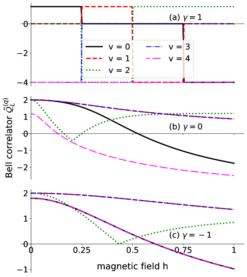
Figure 1: Value of the optimized Bell correlator, $\tilde{\mathcal{Q}}_{L}^{(q)}$, Eq.(24) for an eigenstate $|\psi^{(h)}_{v}\rangle$ of LMG Hamiltonian $\hat{H}_{\gamma}$, as a function of the magnetic field for $L=4$ spins. The black solid line corresponds to the ground state ($v=0$), the red dashed line corresponds to the first excited state ($v=1$), the green dotted line to the $v=2$, the blue dash-dot line to $v=3$, and the magenta long-dashed line to $v=4$.

III.1.2 Analytical expression for $\tilde{\mathcal{E}}_{L}^{(q)}$ for $\gamma=1$

One of our main numerical results is that for all eigenstates the optimal orientation of the two axes defining the rising operators turns out to be

$$\hat{S}^{(x)}_{+}=\hat{S}_{y}+i\hat{S}_{z}.$$ (29)

This operator raises the spin projection along the $x$ axis (as it is expressed in terms of two collective spin operators of directions orthogonal to $x$). The optimal direction for the many-body Bell correlator is consistent with the following observation. The GHZ state obtained with the OAT protocol, i.e., with the Hamiltonian $\propto\hat{S}_{z}^{2}$ Hamiltonian [plodzien2020producing, plodzien2022one], is a superposition as in Eq. (18) with $|0\rangle$ and $|1\rangle$ as eigenstates of $\hat{\sigma}_{x}$ operators. Hence it is the $x$-axis rising operator that is sensitive to this macroscopic superposition .

It is now our goal to express the expectation value of the Bell correlator fed with operator from Eq. (29) on the Dicke states. These are the eigenstates of $\hat{S}_{z}$ hence the calculation requires an additional rotation through the $y$-axis that would align the $x$ and $z$ orientations, i.e.,

$$\hat{S}^{(x)}_{+}=e^{-i\frac{\pi}{2}\hat{S}_{y}}\hat{S}^{(z)}_{+}e^{i\frac{\pi}{2}\hat{S}_{y}}.$$ (30)

The action of such a rotation operator on the Dicke state is

$$e^{i\frac{\pi}{2}\hat{S}_{y}}|S,m\rangle=\sum_{m^{\prime}=-S}^{S}d_{m;m^{\prime}}^{S}\left(\frac{\pi}{2}\right)|S,m^{\prime}\rangle,$$ (31)

where $d_{m;m^{\prime}}^{S}$ represents an element of the Wigner matrix in the fixed-$S$ subspace . As argued below Eq. (20), the Bell correlator is fully determined by the GHZ-coherence, hence by the modulus square of the product of the coefficients multiplying the extreme elements $m^{\prime}=S$ and $m^{\prime}=-S$ in Eq. (31), namely

$$\tilde{\mathcal{E}}_{L}^{(q)}=\left|d_{m;S}^{S}\left(\frac{\pi}{2}\right)d_{m;-S}^{S}\left(\frac{\pi}{2}\right)\right|^{2}=\left[\frac{1}{2^{L}}\binom{L}{m+\frac{L}{2}}\right]^{2}.$$ (32)

When $L$ is large, the binomial can be approximated with the Gaussian, giving

$$\tilde{\mathcal{E}}_{L}^{(q)}\simeq\frac{2}{\pi L}e^{-4\frac{m^{2}}{L}}.$$ (33)

For $m=0$. the Bell limit is surpassed for all $L$, as $\frac{2}{\pi L}>2^{-L}$ for all integer $L$. It is always maximal at $m=0$, hence it is not necessarily the ground state that is most non-classical. In particular, for sufficiently large $h$, the ground state given by Eq. (10) is separable—all the $L$ spins point in the upward direction.

To verify our analytical findings, in Fig. 2, we present $\tilde{\mathcal{Q}}_{L}^{(q)}=\log_{2}(2^{L}\tilde{\mathcal{E}}_{L}^{(q)})$, Eq.(24), as a function of magnetization $m=\langle\hat{S}_{z}\rangle$. For each set of parameters $\{L,h\}$ we calculate all the eigenstates $|\psi_{v}\rangle$ of $\hat{H}_{\gamma=+1}$ and numerically confirm the optimal orientation of Eq. (29). We plot $\tilde{\mathcal{Q}}_{L}^{(q)}$ as a function of $m$, with the blue dots presenting the numerical optimization of the correlator, while the red diamonds corresponding to our analytical findings, Eq. (33). The inverted parabola $\tilde{\mathcal{Q}}_{L}^{(q)}(m)$ shows that maximal Bell correlations are for the eigenstates for which the magnetization is zero, one of important results of the presented work. Note that the normalized Bell correlator $\tilde{\mathcal{Q}}_{L}^{(q)}$ can be linked with the energy from Eq. (6), calculated at $h=0$, as follows

$$\tilde{\mathcal{Q}}_{L}^{(q)}=-\alpha E_{m}+\beta L+\gamma,$$ (34)

where $\alpha=2/\ln 2$, $\beta=1-1/\ln 2$ and $\gamma=\log_{2}\left(\frac{2}{\pi L}\right)-2/\ln 2$. This is a simple formula but of high predictive power, showings the benefit of keeping a string of spins at low energies/temperatures. Note that the Bell correlations are present mostly in the zero- (or close to) magnetization sector; this observation is in an agreement with results of Ref. [Tura2015], where Authors have identified classes of Bell inequalities for which zero magnetization states are optimal. It is important to note that the Dicke states have been experimentally realized for few qubits using various physical platforms, including photonic systems [PhysRevLett.109.173604, PhysRevLett.103.020504, PhysRevA.83.013821, Zhao:15, Wang2016, Mu:20], ultracold atoms [PhysRevLett.112.155304], and quantum circuits [Chakraborty2014, 10.1007/978-3-030-25027-0_9, 9275336, PhysRevLett.103.020503, 9951196, Narisada2023].

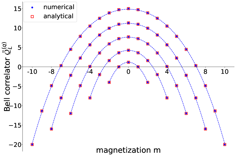
Figure 2: The optimized Bell correlator $\tilde{\mathcal{Q}}_{L}^{(q)}$ (blue dots)for an eigenstate $|\psi^{(h)}_{v}\rangle$ of LMG Hamiltonian $\hat{H}_{\gamma}$, as a function of the magnetization $m=\langle\hat{S}_{z}\rangle$ for $L=4,8,12,16,20$ (from inner to outer lines, respectively). Red squares represent the analytical expression, Eq.(32). Dashed blue lines are to guide an eye.

III.2 Thermal states

The next question we answer is about the impact of thermal fluctuations on the Bell correlations in the LMG models. To investigate this problem, we calculate the thermal density matrix

$$\hat{\varrho}_{T}=\frac{1}{{\cal Z}}\sum_{v}e^{-E_{v}/T}|\psi_{v}\rangle\!\langle\psi_{v}|,$$ (35)

for each $\gamma$, where ${\cal Z}=\sum_{v}e^{-E_{v}/T}$ is the statistical sum and the summation runs over the whole spectrum. Next, we calculate the expectation value of the many-body Bell correlator,

$$\tilde{\mathcal{E}}_{L}^{(q)}(T)=\big{|}\frac{1}{L!}{\rm Tr}\left[\hat{\varrho}_{T}\hat{P}^{\dagger}(\vec{\theta})\hat{S}_{+}^{(x)L}\hat{P}(\vec{\theta})\right]\big{|}^{2}$$ (36)

optimized over $\vec{\theta}$.

In Fig. 3 we show the $\tilde{\mathcal{Q}}_{L}^{(q)}$, Eq. (24), in the $h-T$ plane density plot for $\gamma=1,0,-1$ for given $L$. We observe that for a given temperature, the Bell correlator plotted as a function of $h$ shows a complicated and rich structure, knowledge of which could be relevant for future applications where the performance of a particular task relies on the strength of Bell correlations.

In the following paragraphs, we investigate the origins of those fine structures for the $\gamma=1$ and $\gamma=0$, providing the explanation for

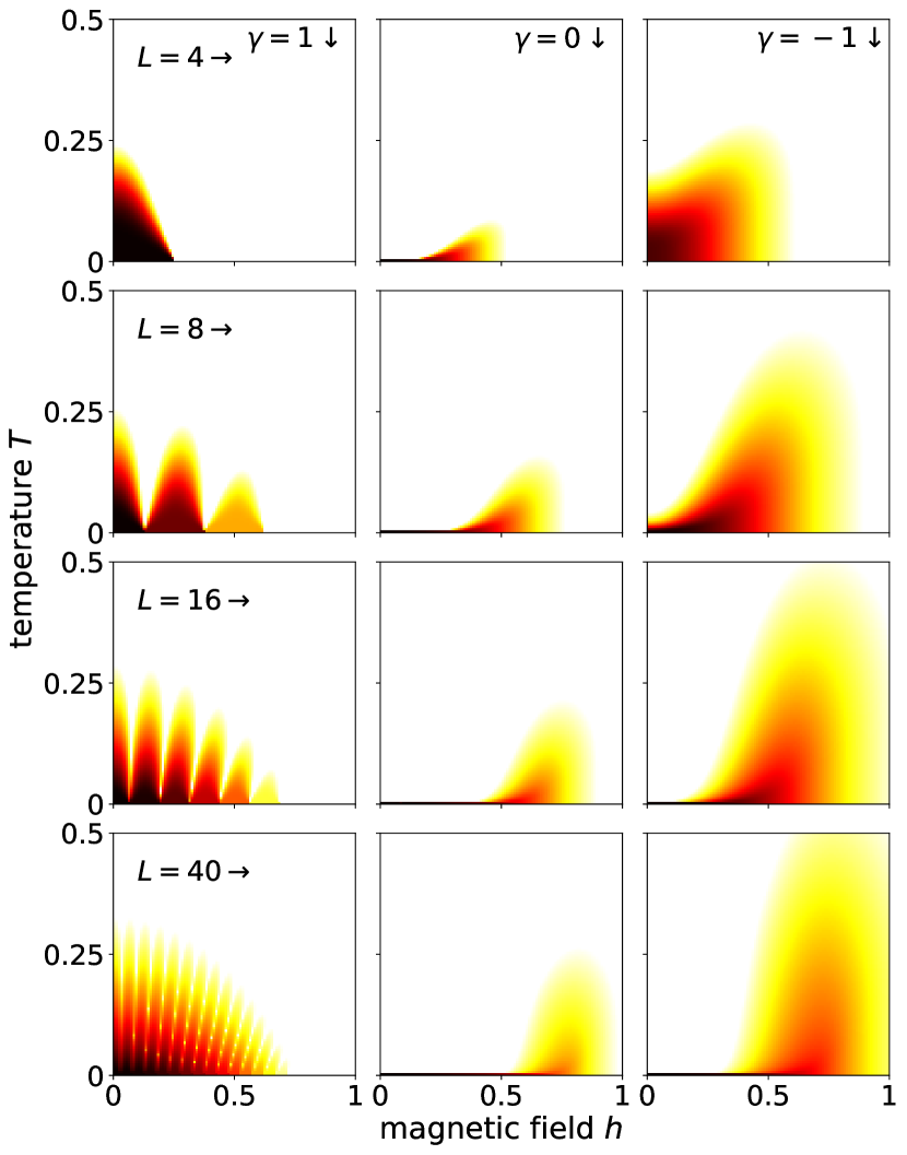
Figure 3: Many-body Bell correlator $\tilde{{\cal Q}}^{(q)}_{L}$ for Gibbs state at temperature $T$ as a function of the magnetic field $h$ for $\gamma=\{1,0,-1\}$ (from left to right, respectively) for $L=4,8,16,40$. White background denotes negative values.

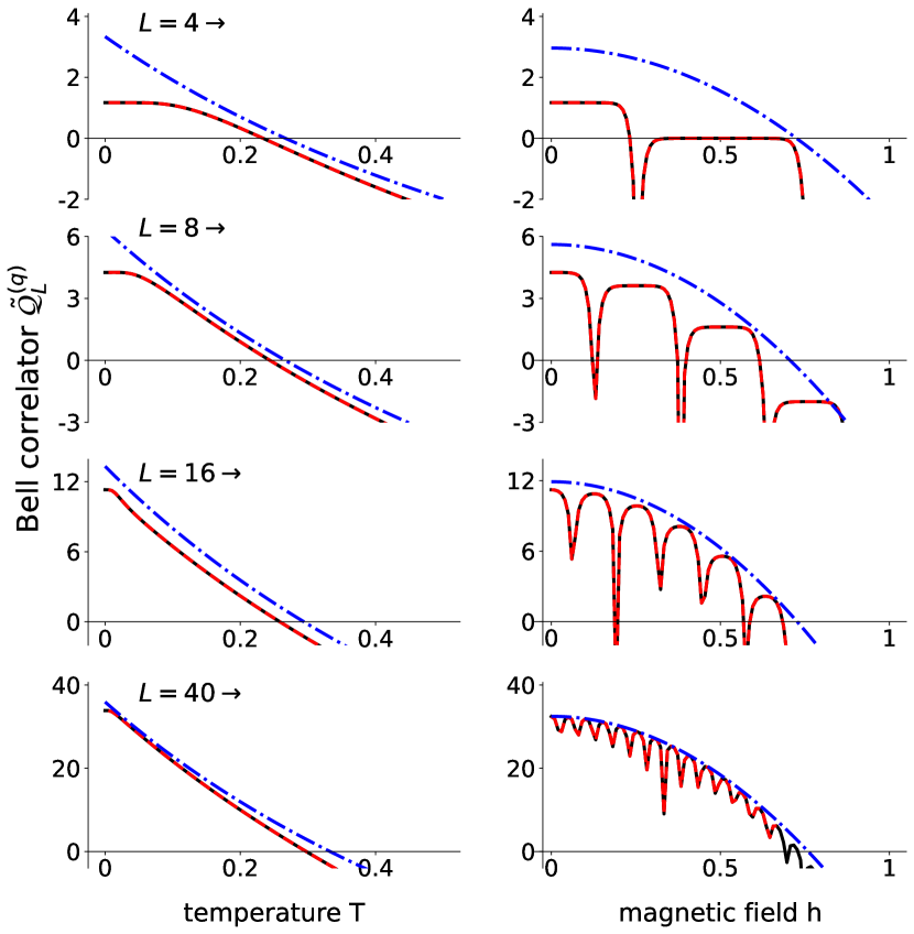
Figure 4: Many-body Bell correlator $\tilde{{\cal Q}}^{(q)}_{L}$ as a function of temperature $T$ (left column) for fixed magnetic field $h=0.04$, and as a function of magnetic field $h$ for fixed temperature $T=0.025$. Rows correspond to system size $L=4,8,16,40$ (from top to bottom, respectively). The black lines correspond to numerical results; red dashed line is the analytical formula from Eq.(38), while the blue dashed-dotted line is the formula obtained in the $L\to\infty$ limit, Eq.(39).

III.2.1 Bell correlator for $T\geqslant 0$ and $\gamma=1$ case

For the $\gamma=1$ case, when the spectrum is spanned by the Dicke states, we have

$$\hat{\varrho}_{T}=\frac{1}{{\cal Z}}\sum_{m=-L/2}^{L/2}e^{-E_{m}/T}|S,m\rangle\langle S,m|,$$ (37)

where the energies are given by Eq. (6). Using Eq. (33) we obtain

$$\tilde{\mathcal{E}}_{L}^{(q)}(T)\simeq\frac{2}{\pi L}\frac{1}{{\cal Z}^{2}}\big{|}\sum_{m=-L/2}^{L/2}(-1)^{m}e^{-\frac{2}{L}(m^{2}-hm)}e^{-\frac{2}{LT}m^{2}}\big{|}^{2},$$ (38)

In Fig.4 we present the fixed-$T$ and fixed-$h$ cuts of the phase diagram shown in Fig.3. The black solid lines corresponds to numerical results, while the red dashed lines to analytical expression, Eq.(38), presenting a perfect agreement even for small $L$. Some more insight into the behavior of $\tilde{\mathcal{E}}_{L}^{(q)}(T)$ from Eq. (38) can be retreived from the large-$L$ limit, where the sum over discrete $m$ is replaced with an integral. Since the $m$’s range from $-L/2$ to $L/2$, extending the corresponding integral limits to $\pm\infty$ requires that the width of the $T$-dependent Gaussian $\sigma=\sqrt{LT}$ remains much smaller than $L$. Hence for the validity of the continuous approximation to hold, the following must be satisfied $T\ll 1/L$. In this regime, the Gaussian integral gives a straightforward outcome

$$\tilde{\mathcal{E}}_{L}^{(q)}(T)=\frac{8}{\pi L(T+1)}e^{-\frac{h^{2}L}{1+T}}e^{-\frac{\pi^{2}LT}{4(1+T)}}.$$ (39)

In Fig.4, we plot $\tilde{\mathcal{Q}}_{L}^{(q)}$ for the above equation as a blue dash-dotted line, which gives an estimate for the envelope for $\tilde{\mathcal{E}}_{L}^{(q)}(T)$, improving as $L$ grows. The structures seen in Figs 3 and 4 as fast oscillations of the correlator as a function of $h$ are lost in the approximation (39). They are a consequence of discrete-$L$ interference effects in Eq. (38). Clearly, as $L$ grows, these structures become denser and finer, and—as expected—are smoothed-out in the $L\gg 1$ limit.

The formula (39) allows for an estimate of the critical temperature $T_{\rm crit}$, above which the Bell correlations vanish for a given $h$. We insert the expression (39) into the inequality Eq. (16) and obtain that

$$T_{\rm crit}=\frac{\ln 2-h^{2}}{\frac{\pi^{2}}{4}-\ln 2}$$ (40)

which is in very good agreement with numerical results, visible in Fig. 4. We stress that the critical temperature does not depend on the system size $L$, as expected from the thermodynamic limit. In particular, when $h=0$ the critical temperature is maximal and equal to $T_{\rm crit}\simeq 0.39$. Moreover, the condition $T_{\rm crit}=0$ gives the maximal $h=\sqrt{\ln 2}\simeq 0.83$ above which the Bell correlations vanish for all $T$, see the blue line in Fig. 4. Note that the $T_{\rm crit}$ obtained from the many-body Bell correlator considered in this work is about $2$ times smaller than the critical temperature reported in [Fadel2018bellcorrelations], based on Bell inequality formed with two-body correlators only.

III.2.2 Bell correlator for $T\geqslant 0$ and $\gamma=0$ case

Some insight into the structure of the $T-h$ graph shown in Fig. 3 can be obtained also for $\gamma=0$. In this case the LMG system can be modelled with an approximate Schrödinger-like equation, as follows. First, we write the stationary Schrodinger equation, acting with the $\hat{H}_{\gamma=0}$ Hamiltonian on the state decomposed in the Dicke basis

$$|\psi\rangle=\sum_{m=-L/2}^{L/2}\psi_{m}|S,m\rangle$$ (41)

which reads

$$-\frac{hL}{2}\left[\psi_{m+1}f_{+}(z_{m})+\psi_{m-1}f_{-}(z_{m})\right]+\frac{L}{4h}\psi_{m}z^{2}_{m}=E\psi_{m}.$$ (42)

Here, we introduced a normalized variable

$$z_{m}=2\frac{m}{L}$$ (43)

that changes between -1 and 1. Also, the coefficients $f_{\pm}(z_{m})$ present in Eq. (42) are defined as follows

$$f_{\pm}(z_{m})=\sqrt{\frac{1\pm z_{m}}{2}\left(\frac{1\mp z_{m}}{2}+\frac{1}{L}\right)}.$$ (44)

Note that we performed the $h\rightarrow-h$ transformation, that can be generated with a local single-spin transformation (rotation of the Hamiltonian around $\hat{S}_{x}$ through an angle equal to $\pi$), which does not modify the Bell content but allows to maintain consistent notation with previous works [ZP2008, hamza2024bell].

For large $L$, the $1/L$ terms in these square-roots can be neglected and $z_{m}$ becomes quasi-continuous, allowing to approximate the difference between the state coefficients $\psi_{m\pm 1}$ with the second derivative over $z$. This gives a Schrödinger-like equation for the wave-function $\psi_{m}\rightarrow\psi(z)$ of a fictitious unit-mass particle

$$\left(-\frac{2}{L}\sqrt{1-z^{2}}\frac{d^{2}}{dz^{2}}+V_{\rm eff}(z)\right)\psi(z)=\tilde{E}\psi(z),$$ (45)

where the effective potential is

$$V_{\rm eff}(z)=-\sqrt{1-z^{2}}+z^{2}\kappa/2$$ (46)

and $\kappa=\frac{1}{h}$. The details of this derivation can be found in Ref. [ZP2008].

Crucially, the spectrum of the Eq. (45) depends on the value of $\kappa$. When it is large, the second term of Eq. (46) dominates giving an effective potential that is close to harmonic. Interestingly, when $\kappa$ surpasses the threshold value $\kappa=-1$, the potential develops two minima located at $\pm z_{0}$, where $z_{0}=(1-1/\kappa^{2})^{1/2}$ and becomes

$$V_{\rm eff}(z)\simeq\frac{1}{2}\kappa(1-\kappa^{2})(z\pm z_{0})^{2}+\mathrm{const.}$$ (47)

The ground state tends to localize around these minima and form a macroscopic superposition

$$\psi_{\rm gr}\simeq\frac{1}{\sqrt{2}}\left[\psi_{0}(z-z_{0})+\psi_{0}(z+z_{0})\right],$$ (48)

where $\psi_{0}(z\pm z_{0})$ is the Gaussian ground state of each of the the harmonic contributions to Eq. (47). When this superposition forms, the Bell correlator $\tilde{\mathcal{Q}}_{L}^{(q)}$ becomes large, as it is exactly this type of macroscopic superposition that it is sensitive to, see Eq. (20). This is why the central column of Fig. 3 shows non-vansing Bell correlator when $h$ is sufficiently small.

However, an important feature of this plot is yet to explained—namely why the $\tilde{\mathcal{Q}}_{L}^{(q)}$ seems more vulnerable to thermal fluctuations when $h$ is very small (i.e., the area of non-zero Bell correlations shrinks with $h\rightarrow 0$).

To explain this behavior, note that as $h$ drops, so that $\kappa\rightarrow-\infty$, the ground state (48) becomes (assymptotically) degenerate with the first excited state

$$\psi_{\rm 1^{st}}\simeq\frac{1}{\sqrt{2}}\left[\psi_{0}(z-z_{0})-\psi_{0}(z+z_{0})\right].$$ (49)

In this regime, any non-zero value of $T$ will lead to occupation of both these states. The GHZ coherences of Eqs (48) and (49) have opposite signs, therefore the Bell correlations quickly degrade in this thermal mixture. This is a qualitative explanation, for a more quantitative analysis, see [hamza2024bell]. When $h\simeq 0$, the ground state is the GHZ state, giving the maximal Bell correlator, but only at $T=0$. This is represented by a very thin and dark line in the central column of Fig. 3.

III.3 Distance-dependent interactions

So far, we considered the LMG model, which is characterized by the constant strength all-to-all interactions, see Eq. (1). We now take a step further and allow for the two-body coupling to depend on the distance between the spins, by considering the following Hamiltonian

$$\hat{H}=-\frac{1}{L}\sum_{i<j}J_{ij}\left(\hat{\sigma}_{x}^{(i)}\hat{\sigma}_{x}^{(j)}+\gamma\hat{\sigma}_{y}^{(i)}\hat{\sigma}_{y}^{(j)}\right)$$ (50)

with the power-law dependence of the coupling strength, i.e., $J_{ij}=|i-j|^{-\alpha}$, with the exponent ranging from $\alpha=0$ (fully connected all-to-all case) to $\alpha\rightarrow\infty$ (nearest-neighbors interaction). While the fully connected models are now realized in experiments, the distance-dependent interactions are still a natural playground for most cases, as in the state-of-the-art quantum simulator platforms   [Zhang2017, doi:10.1126/science.aax9743, bornet2023scalable, Eckner2023, franke2023quantumenhanced, PhysRevX.12.011018, RevModPhys.93.025001, PhysRevLett.131.033604, PhysRevLett.129.063603]. The above Hamiltonian is of particular importance for potential experiments aiming to generate non-classical correlations in spin chains. The behavior of the two-body Bell correlations around the critical value of the transverse-field Ising model has been studied in [Piga2019].

Note that the Hamiltonian from Eq. (50) is absent of the permutational invariance. Hence, we must refer to the single-spin addressing Bell correlator from Eq. (15) or (17) and optimize the orientations of the $\hat{\sigma}_{+}^{(k)}$ operators independently for each $k$, which significantly increases the computational load. In Fig. 5 we present the optimized Bell correlation for the ground state and using finite $\alpha$, normalized to the value obtained with the all-to-all case (i.e., such that can be reproduced by setting $\alpha=0$). The blue dashed line shows the constant $\alpha$-independent normalized Bell correlations for $\gamma=0$, while the solid red and dot-dashed black line present a decaying Bell correlator for $\gamma=1$ and $-1$, respectively.

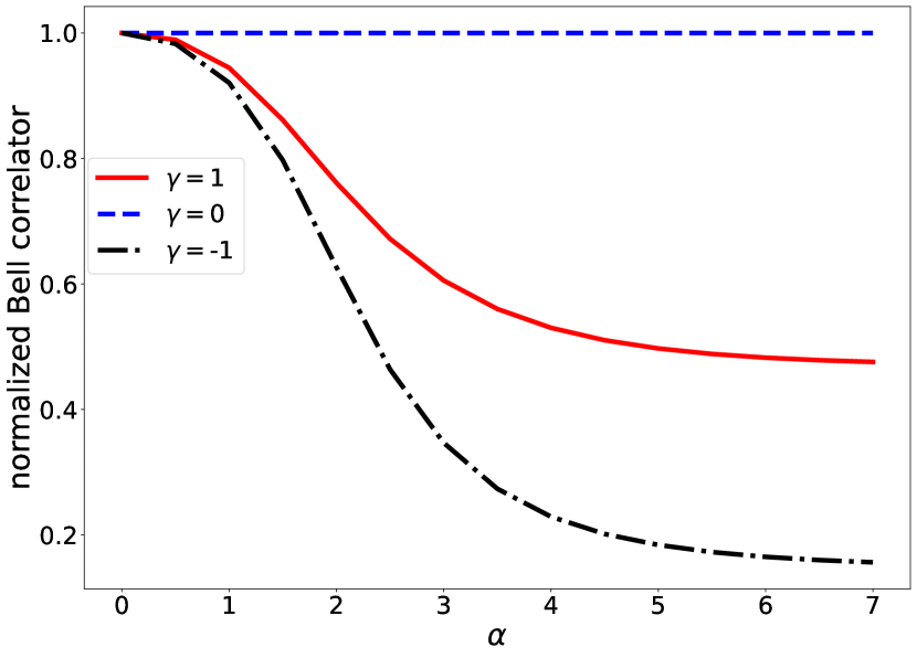
Figure 5: Many-body Bell correlator calculated with the ground state for the distance-dependent interactions with $L=8$. The dashed blue line is for $\gamma=0$, the solid red line for $\gamma=1$ and the dot-dashed black line is for $\gamma=-1$.

A particularly instructive case is for infinitesimally small $\gamma$’s. We start with the $\gamma=0$ case, giving the Hamiltonian

$$\hat{H}=-\frac{1}{L}\sum_{i<j}J_{ij}\hat{\sigma}_{x}^{(i)}\hat{\sigma}_{x}^{(j)}.$$ (51)

Due to the presence of the minus sign in front, the minimal energy when the sum is maximal, i.e., when the spins all’unisono point either “up” or “down”. The doubly degenerate ground state is either $|0\rangle_{x}^{\otimes L}$ or $|1\rangle_{x}^{\otimes L}$. Both are fully separable, a consequence of the classical structure of the Hamiltonian Eq.(51), only involving operators $\hat{\sigma}_{x}$. However, even infinitesimal $\gamma$ lifts the ground state degeneracy. As a result, the GHZ states

$$|\psi_{\pm}\rangle=\frac{1}{\sqrt{2}}(|0\rangle_{x}^{\otimes L}\pm|1\rangle_{x}^{\otimes L}),$$ (52)

become of minimal energy. Such highly entangled states give the maximal value of the correlator, see the discussion around Eq. (18) (for detailed discussion of the quantum Ising ground state see [Parkinson2010, mbeng2020quantum]) Note that this argument holds for all $\alpha$’s, a consequence of the minus sign in front of the sum in the Hamiltonian (51).

The other cases, $\gamma=\pm 1$, call for a numerical-only approach and, as shown in Fig. 5, the dependence of $\alpha$ is strongly pronounced.

III.4 Diagonal and off-diagonal disorder

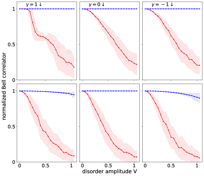
Figure 6: Relative change of the Bell correlations in the ground state, as a function of disorder amplitude. The red lines with shaded areas correspond to diagonal disorder, while the blue lines (with shaded area, not visible) correspond to off-diagonal disorder. The Bell correlations are robust to off-diagonal disorder, and preserved with diagonal disorder. Top row shows the impact of the uniform distribution ${\cal P}^{(1)}$ while the bottom row is for the experimental distribution ${\cal P}^{(2)}$. The number of spins is $L=8$

In this last section, we enrich the above distance-dependent model, taking into account non-vanishing $h$, namely

$$\hat{H}=-\frac{1}{L}\sum_{i<j}J_{ij}\left(\hat{\sigma}_{x}^{(i)}\hat{\sigma}_{x}^{(j)}+\gamma\hat{\sigma}_{y}^{(i)}\hat{\sigma}_{y}^{(j)}\right)+\sum_{i}h_{i}\hat{\sigma}_{z}^{(i)}$$ (53)

and allowing for the presence of fluctuations of both $h_{i}$ (called the diagonal disorder) and of the spin couplings $J_{ij}$ (the off-diagonal disorder). Such fluctuations are inevitable in realistic configurations hence it is of importance to perform a numerical analysis of their influence on the Bell correlator.

We consider two types of probability distributions that generate the noisy random variable $\epsilon$ added to either $h$ or $J_{ij}$, i.e. $h_{i}=\epsilon$ or $J_{ij}=J_{ji}=1+\epsilon$. These are, the uniform distribution from $-V/2$ to $V/2$, i.e.,

$$\mathcal{P}^{(1)}_{a}(\epsilon)=\frac{V}{2}[-1,1]$$ (54)

and alternatively, the probability distribution given by

$$\mathcal{P}^{(2)}_{a}(\epsilon)=\frac{1}{\pi\sqrt{\epsilon(V-\epsilon)}}.$$ (55)

This former type of noise was recently generated and analyzed in the experimental realization of the random-spins models in an optical cavity [Sauerwein2023]. The Fig. 6 summarizes the results for the ground state and for three the cases of $\gamma$ and $\mathcal{P}^{(i)}_{a}(\epsilon)$, showing a general tendency—Bell correlations are robust to off-diagonal disorder. Also, we note that Bell correlations are weakly affected by the diagonal disorder as long as its amplitude is much smaller than $V\ll 1$.

IV Outlook and Conclusions

This work addressed the problem of generating the strongest possible and scalable many-body quantum correlations in spin-$1/2$ chains. We showed that the creation of quantum states with strong many-body Bell correlations does not necessarily have to be done via dynamical protocols such as one-axis twisting.

We showed that many-body Bell correlations are inherently present in the eigenstates of a broad family of spin-$1/2$ models described by the Lipkin-spin-$1/2$ Glick-Meskhov model with all-to-all and power-law interacting spin-$1/2$ models. Next, we showed that inherent many-body Bell correlations are also present in the thermal states of the LMG model, and we estimated the critical temperature above which Bell correlations vanish for the one-axis twisting Hamiltonian. Finally, we showed that the many-body Bell correlations are robust to disorder the potential. We hope that this work shed some light on the properties of the many-body Bell correlations beyond the pure state description [Fadel2018bellcorrelations, PhysRevA.105.L060201].

The remaining question is whether there are possibilities of experimental certification of the many-body Bell correlations in the quantum systems. The measurement of the off-diagonal GHZ element of the density matrix in $L=4$ qubit system has been prepared experimentally in element [Sackett2000]. Recently it was shown the many-body Bell correlations can be extracted with the quantum state tomography via the classical shadows technique [plodzien2024generation] up to $L=10$ spins. Another approach is a technique based on multiple quantum coherence [garttner2017measuring, PhysRevLett.120.040402], which allows to access to individual elements of the density matrix, including those that encode information about many-body Bell correlations.

References

- Einstein et al. [1935] A. Einstein, B. Podolsky, and N. Rosen, Can quantum-mechanical description of physical reality be considered complete?, Phys. Rev. 47, 777 (1935).
- Schrödinger [1935] E. Schrödinger, Die gegenwärtige Situation in der Quantenmechanik, Naturwissenschaften 23, 807 (1935).
- Horodecki et al. [2009] R. Horodecki, P. Horodecki, M. Horodecki, and K. Horodecki, Quantum entanglement, Rev. Mod. Phys. 81, 865 (2009).
- Uola et al. [2020] R. Uola, A. C. S. Costa, H. C. Nguyen, and O. Gühne, Quantum steering, Rev. Mod. Phys. 92, 015001 (2020).
- Bell [1964] J. S. Bell, On the einstein podolsky rosen paradox, Physics 1, 195 (1964).
- Brunner et al. [2014] N. Brunner, D. Cavalcanti, S. Pironio, V. Scarani, and S. Wehner, Bell nonlocality, Rev. Mod. Phys. 86, 419 (2014).
- Frérot et al. [2023] I. Frérot, M. Fadel, and M. Lewenstein, Probing quantum correlations in many-body systems: a review of scalable methods, Reports on Progress in Physics 86, 114001 (2023).
- Srivastava et al. [2024] A. K. Srivastava, G. Müller-Rigat, M. Lewenstein, and G. Rajchel-Mieldzioć, Introduction to quantum entanglement in many-body systems (2024), arXiv:2402.09523 [quant-ph] .
- Knips et al. [2016] L. Knips, C. Schwemmer, N. Klein, M. Wieśniak, and H. Weinfurter, Multipartite entanglement detection with minimal effort, Phys. Rev. Lett. 117, 210504 (2016).
- Acín et al. [2018] A. Acín, I. Bloch, H. Buhrman, T. Calarco, C. Eichler, J. Eisert, D. Esteve, N. Gisin, S. J. Glaser, F. Jelezko, S. Kuhr, M. Lewenstein, M. F. Riedel, P. O. Schmidt, R. Thew, A. Wallraff, I. Walmsley, and F. K. Wilhelm, The quantum technologies roadmap: a european community view, New Journal of Physics 20, 080201 (2018).
- Eisert et al. [2020] J. Eisert, D. Hangleiter, N. Walk, I. Roth, D. Markham, R. Parekh, U. Chabaud, and E. Kashefi, Quantum certification and benchmarking, Nature Reviews Physics 2, 382 (2020).
- Kinos et al. [2021] A. Kinos, D. Hunger, R. Kolesov, K. Mølmer, H. de Riedmatten, P. Goldner, A. Tallaire, L. Morvan, P. Berger, S. Welinski, K. Karrai, L. Rippe, S. Kröll, and A. Walther, Roadmap for rare-earth quantum computing (2021).
- Tavakoli [2020] A. Tavakoli, Semi-device-independent certification of independent quantum state and measurement devices, Phys. Rev. Lett. 125, 150503 (2020).
- Laucht et al. [2021] A. Laucht, F. Hohls, N. Ubbelohde, M. F. Gonzalez-Zalba, D. J. Reilly, S. Stobbe, T. Schröder, P. Scarlino, J. V. Koski, A. Dzurak, C.-H. Yang, J. Yoneda, F. Kuemmeth, H. Bluhm, J. Pla, C. Hill, J. Salfi, A. Oiwa, J. T. Muhonen, E. Verhagen, M. D. LaHaye, H. H. Kim, A. W. Tsen, D. Culcer, A. Geresdi, J. A. Mol, V. Mohan, P. K. Jain, and J. Baugh, Roadmap on quantum nanotechnologies, Nanotechnology 32, 162003 (2021).
- Becher et al. [2022] C. Becher, W. Gao, S. Kar, C. Marciniak, T. Monz, J. G. Bartholomew, P. Goldner, H. Loh, E. Marcellina, K. E. J. Goh, T. S. Koh, B. Weber, Z. Mu, J.-Y. Tsai, Q. Yan, S. Gyger, S. Steinhauer, and V. Zwiller, 2022 roadmap for materials for quantum technologies (2022).
- Fraxanet et al. [2022] J. Fraxanet, T. Salamon, and M. Lewenstein, The coming decades of quantum simulation (2022).
- Sotnikov et al. [2022] O. M. Sotnikov, I. A. Iakovlev, A. A. Iliasov, M. I. Katsnelson, A. A. Bagrov, and V. V. Mazurenko, Certification of quantum states with hidden structure of their bitstrings, npj Quantum Information 8, 41 (2022).
- Huang et al. [2024] H.-Y. Huang, J. Preskill, and M. Soleimanifar, Certifying almost all quantum states with few single-qubit measurements (2024), arXiv:2404.07281 [quant-ph] .
- Kliesch and Roth [2021] M. Kliesch and I. Roth, Theory of quantum system certification, PRX Quantum 2, 010201 (2021).
- Kitagawa and Ueda [1993] M. Kitagawa and M. Ueda, Squeezed spin states, Phys. Rev. A 47, 5138 (1993).
- Wineland et al. [1994] D. Wineland, J. Bollinger, W. Itano, and D. Heinzen, Squeezed atomic states and projection noise in spectroscopy, Phys. Rev. A 50, 67 (1994).
- Korbicz et al. [2005] J. K. Korbicz, J. I. Cirac, and M. Lewenstein, Spin squeezing inequalities and entanglement of qubit states, Phys. Rev. Lett. 95, 120502 (2005).
- Tura et al. [2014a] J. Tura, R. Augusiak, A. B. Sainz, T. Vértesi, M. Lewenstein, and A. Acín, Detecting nonlocality in many-body quantum states, Science 344, 1256 (2014a), https://www.science.org/doi/pdf/10.1126/science.1247715 .
- Tura et al. [2014b] J. Tura, A. B. Sainz, T. Vértesi, A. Acín, M. Lewenstein, and R. Augusiak, Translationally invariant multipartite bell inequalities involving only two-body correlators, Journal of Physics A: Mathematical and Theoretical 47, 424024 (2014b).
- Tura et al. [2015] J. Tura, R. Augusiak, A. Sainz, B. Lücke, C. Klempt, M. Lewenstein, and A. Acín, Nonlocality in many-body quantum systems detected with two-body correlators, Annals of Physics 362, 370 (2015).
- Tura et al. [2019] J. Tura, A. Aloy, F. Baccari, A. Acín, M. Lewenstein, and R. Augusiak, Optimization of device-independent witnesses of entanglement depth from two-body correlators, Phys. Rev. A 100, 032307 (2019).
- Baccari et al. [2019] F. Baccari, J. Tura, M. Fadel, A. Aloy, J.-D. Bancal, N. Sangouard, M. Lewenstein, A. Acín, and R. Augusiak, Bell correlation depth in many-body systems, Phys. Rev. A 100, 022121 (2019).
- Aloy et al. [2021] A. Aloy, M. Fadel, and J. Tura, The quantum marginal problem for symmetric states: applications to variational optimization, nonlocality and self-testing, New Journal of Physics 23, 033026 (2021).
- Müller-Rigat et al. [2021] G. Müller-Rigat, A. Aloy, M. Lewenstein, and I. Frérot, Inferring nonlinear many-body bell inequalities from average two-body correlations: Systematic approach for arbitrary spin- ensembles, PRX Quantum 2, 030329 (2021).
- Marconi et al. [2022] C. Marconi, A. Riera-Campeny, A. Sanpera, and A. Aloy, Robustness of nonlocality in many-body open quantum systems, Phys. Rev. A 105, L060201 (2022).
- Mermin [1990] N. D. Mermin, Extreme quantum entanglement in a superposition of macroscopically distinct states, Phys. Rev. Lett. 65, 1838 (1990).
- Schmid et al. [2008] C. Schmid, N. Kiesel, W. Laskowski, W. Wieczorek, M. Żukowski, and H. Weinfurter, Discriminating multipartite entangled states, Phys. Rev. Lett. 100, 200407 (2008).
- Żukowski and Brukner [2002] M. Żukowski and i. c. v. Brukner, Bell’s theorem for general n-qubit states, Phys. Rev. Lett. 88, 210401 (2002).
- Cavalcanti et al. [2007a] E. G. Cavalcanti, C. J. Foster, M. D. Reid, and P. D. Drummond, Bell inequalities for continuous-variable correlations, Phys. Rev. Lett. 99, 210405 (2007a).
- Reid et al. [2012] M. D. Reid, Q.-Y. He, and P. D. Drummond, Entanglement and nonlocality in multi-particle systems, Frontiers of Physics 7, 72 (2012).
- Cavalcanti et al. [2011a] E. G. Cavalcanti, Q. Y. He, M. D. Reid, and H. M. Wiseman, Unified criteria for multipartite quantum nonlocality, Phys. Rev. A 84, 032115 (2011a).
- Guo et al. [2023] J. Guo, J. Tura, Q. He, and M. Fadel, Detecting bell correlations in multipartite non-gaussian spin states, Phys. Rev. Lett. 131, 070201 (2023).
- Płodzień et al. [2020] M. Płodzień, M. Kościelski, E. Witkowska, and A. Sinatra, Producing and storing spin-squeezed states and greenberger-horne-zeilinger states in a one-dimensional optical lattice, Physical Review A 102, 013328 (2020).
- Płodzień et al. [2022] M. Płodzień, M. Lewenstein, E. Witkowska, and J. Chwedeńczuk, One-axis twisting as a method of generating many-body bell correlations, Physical Review Letters 129, 250402 (2022).
- Hernández Yanes et al. [2022] T. Hernández Yanes, M. Płodzień, M. Mackoit Sinkevičienė, G. Žlabys, G. Juzeliūnas, and E. Witkowska, One- and two-axis squeezing via laser coupling in an atomic fermi-hubbard model, Phys. Rev. Lett. 129, 090403 (2022).
- Dziurawiec et al. [2023] M. Dziurawiec, T. Hernández Yanes, M. Płodzień, M. Gajda, M. Lewenstein, and E. Witkowska, Accelerating many-body entanglement generation by dipolar interactions in the bose-hubbard model, Phys. Rev. A 107, 013311 (2023).
- Hernández Yanes et al. [2023] T. Hernández Yanes, G. Žlabys, M. Płodzień, D. Burba, M. M. Sinkevičienė, E. Witkowska, and G. Juzeliūnas, Spin squeezing in open heisenberg spin chains, Phys. Rev. B 108, 104301 (2023).
- Płodzień et al. [2024] M. Płodzień, T. Wasak, E. Witkowska, M. Lewenstein, and J. Chwedeńczuk, Generation of scalable many-body bell correlations in spin chains with short-range two-body interactions, Physical Review Research 6, 023050 (2024).
- Yanes et al. [2024] T. H. Yanes, A. Niezgoda, and E. Witkowska, Exploring spin-squeezing in the mott insulating regime: role of anisotropy, inhomogeneity and hole doping (2024), arXiv:2403.06521 [cond-mat.quant-gas] .
- Schmied et al. [2016] R. Schmied, J.-D. Bancal, B. Allard, M. Fadel, V. Scarani, P. Treutlein, and N. Sangouard, Bell correlations in a bose-einstein condensate, Science 352, 441 (2016), https://www.science.org/doi/pdf/10.1126/science.aad8665 .
- Engelsen et al. [2017] N. J. Engelsen, R. Krishnakumar, O. Hosten, and M. A. Kasevich, Bell correlations in spin-squeezed states of 500 000 atoms, Phys. Rev. Lett. 118, 140401 (2017).
- Pezzè et al. [2018] L. Pezzè, A. Smerzi, M. K. Oberthaler, R. Schmied, and P. Treutlein, Quantum metrology with nonclassical states of atomic ensembles, Rev. Mod. Phys. 90, 035005 (2018).
- Wolfgramm et al. [2010] F. Wolfgramm, A. Cere, F. A. Beduini, A. Predojević, M. Koschorreck, and M. W. Mitchell, Squeezed-light optical magnetometry, Physical review letters 105, 053601 (2010).
- Müller-Rigat et al. [2023] G. Müller-Rigat, A. K. Srivastava, S. Kurdziałek, G. Rajchel-Mieldzioć, M. Lewenstein, and I. Frérot, Certifying the quantum fisher information from a given set of mean values: a semidefinite programming approach, Quantum 7, 1152 (2023).
- Lipkin et al. [1965] H. Lipkin, N. Meshkov, and A. Glick, Validity of many-body approximation methods for a solvable model: (i). exact solutions and perturbation theory, Nuclear Physics 62, 188 (1965).
- Meshkov et al. [1965] N. Meshkov, A. Glick, and H. Lipkin, Validity of many-body approximation methods for a solvable model: (ii). linearization procedures, Nuclear Physics 62, 199 (1965).
- Glick et al. [1965] A. Glick, H. Lipkin, and N. Meshkov, Validity of many-body approximation methods for a solvable model: (iii). diagram summations, Nuclear Physics 62, 211 (1965).
- Botet et al. [1982] R. Botet, R. Jullien, and P. Pfeuty, Size scaling for infinitely coordinated systems, Phys. Rev. Lett. 49, 478 (1982).
- Lerma-H and Dukelsky [2014] S. Lerma-H and J. Dukelsky, The lipkin-meshkov-glick model from the perspective of the su(1,1) richardson-gaudin models, Journal of Physics: Conference Series 492, 012013 (2014).
- Botet and Jullien [1983] R. Botet and R. Jullien, Large-size critical behavior of infinitely coordinated systems, Phys. Rev. B 28, 3955 (1983).
- Carrasco et al. [2016] J. A. Carrasco, F. Finkel, A. González-López, M. A. Rodríguez, and P. Tempesta, Generalized isotropic lipkin–meshkov–glick models: ground state entanglement and quantum entropies, Journal of Statistical Mechanics: Theory and Experiment 2016, 033114 (2016).
- Huang et al. [2018a] Y. Huang, T. Li, and Z.-q. Yin, Symmetry-breaking dynamics of the finite-size lipkin-meshkov-glick model near ground state, Phys. Rev. A 97, 012115 (2018a).
- Hammam et al. [2024] K. Hammam, G. Manzano, and G. De Chiara, Quantum coherence enables hybrid multitask and multisource regimes in autonomous thermal machines, Phys. Rev. Res. 6, 013310 (2024).
- Farina et al. [2024] D. Farina, B. Benazout, F. Centrone, and A. Acín, Thermodynamic precision in the nonequilibrium exchange scenario, Phys. Rev. E 109, 034112 (2024).
- He et al. [2012] X. He, J. He, and J. Zheng, Thermal entangled quantum heat engine, Physica A: Statistical Mechanics and its Applications 391, 6594 (2012).
- Ma et al. [2017] Y.-H. Ma, S.-H. Su, and C.-P. Sun, Quantum thermodynamic cycle with quantum phase transition, Phys. Rev. E 96, 022143 (2017).
- Huang et al. [2018b] X. Huang, Q. Sun, D. Guo, and Q. Yu, Quantum otto heat engine with three-qubit xxz model as working substance, Physica A: Statistical Mechanics and its Applications 491, 604 (2018b).
- Łobejko et al. [2020] M. Łobejko, P. Mazurek, and M. Horodecki, Thermodynamics of Minimal Coupling Quantum Heat Engines, Quantum 4, 375 (2020).
- Çakmak et al. [2020] S. Çakmak, M. Çandır, and F. Altintas, Construction of a quantum carnot heat engine cycle, Quantum Information Processing 19, 314 (2020).
- Hartmann et al. [2020] A. Hartmann, V. Mukherjee, W. Niedenzu, and W. Lechner, Many-body quantum heat engines with shortcuts to adiabaticity, Phys. Rev. Res. 2, 023145 (2020).
- Chen et al. [2019] Y.-Y. Chen, G. Watanabe, Y.-C. Yu, X.-W. Guan, and A. del Campo, An interaction-driven many-particle quantum heat engine and its universal behavior, npj Quantum Information 5, 88 (2019).
- Centamori et al. [2023] E. M. Centamori, M. Campisi, and V. Giovannetti, Spin-chain based quantum thermal machines (2023), arXiv:2303.15574 [quant-ph] .
- Chakour et al. [2021] M. H. B. Chakour, A. E. Allati, and Y. Hassouni, Entangled quantum refrigerator based on two anisotropic spin-1/2 heisenberg xyz chain with dzyaloshinskii–moriya interaction, The European Physical Journal D 75, 42 (2021).
- Melo et al. [2022] F. V. Melo, N. Sá, I. Roditi, A. M. Souza, I. S. Oliveira, R. S. Sarthour, and G. T. Landi, Implementation of a two-stroke quantum heat engine with a collisional model, Phys. Rev. A 106, 032410 (2022).
- Solfanelli et al. [2023] A. Solfanelli, G. Giachetti, M. Campisi, S. Ruffo, and N. Defenu, Quantum heat engine with long-range advantages, New Journal of Physics 25, 033030 (2023).
- Williamson and Davis [2024] L. A. Williamson and M. J. Davis, Many-body enhancement in a spin-chain quantum heat engine, Phys. Rev. B 109, 024310 (2024).
- Vidal et al. [2004] J. Vidal, G. Palacios, and C. Aslangul, Entanglement dynamics in the lipkin-meshkov-glick model, Phys. Rev. A 70, 062304 (2004).
- Latorre et al. [2005] J. I. Latorre, R. Orús, E. Rico, and J. Vidal, Entanglement entropy in the lipkin-meshkov-glick model, Phys. Rev. A 71, 064101 (2005).
- Orús et al. [2008] R. Orús, S. Dusuel, and J. Vidal, Equivalence of critical scaling laws for many-body entanglement in the lipkin-meshkov-glick model, Phys. Rev. Lett. 101, 025701 (2008).
- Sen [De] A. Sen(De) and U. Sen, Entanglement mean field theory: Lipkin–meshkov–glick model, Quantum Information Processing 11, 675 (2012).
- Wang et al. [2012] C. Wang, Y.-Y. Zhang, and Q.-H. Chen, Quantum correlations in collective spin systems, Phys. Rev. A 85, 052112 (2012).
- Lourenço et al. [2020] A. C. Lourenço, S. Calegari, T. O. Maciel, T. Debarba, G. T. Landi, and E. I. Duzzioni, Genuine multipartite correlations distribution in the criticality of the lipkin-meshkov-glick model, Phys. Rev. B 101, 054431 (2020).
- Hengstenberg et al. [2023] S. M. Hengstenberg, C. E. P. Robin, and M. J. Savage, Multi-body entanglement and information rearrangement in nuclear many-body systems: a study of the lipkin–meshkov–glick model, The European Physical Journal A 59, 231 (2023).
- Bao et al. [2020] J. Bao, B. Guo, Y.-H. Liu, L.-H. Shen, and Z.-Y. Sun, Multipartite nonlocality and global quantum discord in the antiferromagnetic lipkin–meshkov–glick model, Physica B: Condensed Matter 593, 412297 (2020).
- and et al. [2011] and, , and and, Thermal entanglement in lipkin—meshkov—glick model, Communications in Theoretical Physics 56, 61 (2011).
- Shao and Fu [2024] L. Shao and L. Fu, Spin squeezing generated by the anisotropic central spin model, Phys. Rev. A 109, 052618 (2024).
- Chen et al. [2009] G. Chen, J. Q. Liang, and S. Jia, Interaction-induced lipkin-meshkov-glick model in a bose-einstein condensate inside an optical cavity, Opt. Express 17, 19682 (2009).
- Larson [2010] J. Larson, Circuit qed scheme for the realization of the lipkin-meshkov-glick model, Europhysics Letters 90, 54001 (2010).
- Sauerwein et al. [2023] N. Sauerwein, F. Orsi, P. Uhrich, S. Bandyopadhyay, F. Mattiotti, T. Cantat-Moltrecht, G. Pupillo, P. Hauke, and J.-P. Brantut, Engineering random spin models with atoms in a high-finesse cavity, Nature Physics 19, 1128 (2023).
- Yang and Jacob [2019] L.-P. Yang and Z. Jacob, Engineering first-order quantum phase transitions for weak signal detection, Journal of Applied Physics 126, 174502 (2019), https://pubs.aip.org/aip/jap/article-pdf/doi/10.1063/1.5121558/15237507/174502_1_online.pdf .
- Morrison and Parkins [2008] S. Morrison and A. S. Parkins, Dynamical quantum phase transitions in the dissipative lipkin-meshkov-glick model with proposed realization in optical cavity qed, Phys. Rev. Lett. 100, 040403 (2008).
- Grimsmo and Parkins [2013] A. L. Grimsmo and A. S. Parkins, Dissipative dicke model with nonlinear atom–photon interaction, Journal of Physics B: Atomic, Molecular and Optical Physics 46, 224012 (2013).
- Gelhausen and Buchhold [2018] J. Gelhausen and M. Buchhold, Dissipative dicke model with collective atomic decay: Bistability, noise-driven activation, and the nonthermal first-order superradiance transition, Phys. Rev. A 97, 023807 (2018).
- Hobday, Isaac et al. [2023] Hobday, Isaac, Stevenson, Paul, and Benstead, James, Variance minimisation on a quantum computer of the lipkin-meshkov-glick model with three particles, EPJ Web of Conf. 284, 16002 (2023).
- Hobday et al. [2024] I. Hobday, P. Stevenson, and J. Benstead, Variance minimisation of the lipkin-meshkov-glick model on a quantum computer (2024), arXiv:2403.08625 [quant-ph] .
- Lourenço et al. [2024] A. C. Lourenço, D. R. Candido, and E. I. Duzzioni, Genuine -partite correlations and entanglement in the ground state of the dicke model for interacting qubits (2024), arXiv:2405.12916 [quant-ph] .
- Żukowski and Brukner [2002] M. Żukowski and Č. Brukner, Bell’s theorem for general n-qubit states, Phys. Rev. Lett. 88, 210401 (2002).
- Cavalcanti et al. [2007b] E. G. Cavalcanti, C. J. Foster, M. D. Reid, and P. D. Drummond, Bell inequalities for continuous-variable correlations, Phys. Rev. Lett. 99, 210405 (2007b).
- He et al. [2011] Q. He, P. Drummond, and M. Reid, Entanglement, epr steering, and bell-nonlocality criteria for multipartite higher-spin systems, Phys. Rev. A 83, 032120 (2011).
- He et al. [2010] Q. He, E. Cavalcanti, M. Reid, and P. Drummond, Bell inequalities for continuous-variable measurements, Phys. Rev. A 81, 062106 (2010).
- Cavalcanti et al. [2011b] E. Cavalcanti, Q. He, M. Reid, and H. Wiseman, Unified criteria for multipartite quantum nonlocality, Phys. Rev. A 84, 032115 (2011b).
- Niezgoda et al. [2020] A. Niezgoda, M. Panfil, and J. Chwedeńczuk, Quantum correlations in spin chains, Phys. Rev. A 102, 042206 (2020).
- Niezgoda and Chwedeńczuk [2021] A. Niezgoda and J. Chwedeńczuk, Many-body nonlocality as a resource for quantum-enhanced metrology, Phys. Rev. Lett. 126, 210506 (2021).
- Płodzień et al. [2022] M. Płodzień, M. Lewenstein, E. Witkowska, and J. Chwedeńczuk, One-Axis Twisting as a Method of Generating Many-Body Bell Correlations, Phys. Rev. Lett. 129, 250402 (2022).
- Chwedenczuk [2022] J. Chwedenczuk, Many-body Bell inequalities for bosonic qubits, SciPost Phys. Core 5, 025 (2022).
- Note [1] From now on, to distinguish between the different orientations of the rising operators, we add the proper superscript [here ].
- Note [2] See [varshalovich1988quantum] for the details on the rotation matrices in the SU(2) group.
- Chiuri et al. [2012] A. Chiuri, C. Greganti, M. Paternostro, G. Vallone, and P. Mataloni, Experimental quantum networking protocols via four-qubit hyperentangled dicke states, Phys. Rev. Lett. 109, 173604 (2012).
- Wieczorek et al. [2009] W. Wieczorek, R. Krischek, N. Kiesel, P. Michelberger, G. Tóth, and H. Weinfurter, Experimental entanglement of a six-photon symmetric dicke state, Phys. Rev. Lett. 103, 020504 (2009).
- Vanderbruggen et al. [2011] T. Vanderbruggen, S. Bernon, A. Bertoldi, A. Landragin, and P. Bouyer, Spin-squeezing and dicke-state preparation by heterodyne measurement, Phys. Rev. A 83, 013821 (2011).
- Zhao et al. [2015] Y.-Y. Zhao, Y.-C. Wu, G.-Y. Xiang, C.-F. Li, and G.-C. Guo, Experimental violation of the local realism for four-qubit dicke state, Opt. Express 23, 30491 (2015).
- Wang et al. [2016] M.-Y. Wang, F.-L. Yan, and T. Gao, Deterministic distribution of four-photon dicke state over an arbitrary collective-noise channel with cross-kerr nonlinearity, Scientific Reports 6, 29853 (2016).
- Mu et al. [2020] F. Mu, Y. Gao, H. Yin, and G. Wang, Dicke state generation via selective interactions in a dicke-stark model, Opt. Express 28, 39574 (2020).
- Lücke et al. [2014] B. Lücke, J. Peise, G. Vitagliano, J. Arlt, L. Santos, G. Tóth, and C. Klempt, Detecting multiparticle entanglement of dicke states, Phys. Rev. Lett. 112, 155304 (2014).
- Chakraborty et al. [2014] K. Chakraborty, B.-S. Choi, A. Maitra, and S. Maitra, Efficient quantum algorithms to construct arbitrary dicke states, Quantum Information Processing 13, 2049 (2014).
- Bärtschi and Eidenbenz [2019] A. Bärtschi and S. Eidenbenz, Deterministic preparation of dicke states, in Fundamentals of Computation Theory: 22nd International Symposium, FCT 2019, Copenhagen, Denmark, August 12-14, 2019, Proceedings (Springer-Verlag, Berlin, Heidelberg, 2019) p. 126–139.
- Mukherjee et al. [2020] C. S. Mukherjee, S. Maitra, V. Gaurav, and D. Roy, Preparing dicke states on a quantum computer, IEEE Transactions on Quantum Engineering 1, 1 (2020).
- Prevedel et al. [2009] R. Prevedel, G. Cronenberg, M. S. Tame, M. Paternostro, P. Walther, M. S. Kim, and A. Zeilinger, Experimental realization of dicke states of up to six qubits for multiparty quantum networking, Phys. Rev. Lett. 103, 020503 (2009).
- Bärtschi and Eidenbenz [2022] A. Bärtschi and S. Eidenbenz, Short-depth circuits for dicke state preparation, in 2022 IEEE International Conference on Quantum Computing and Engineering (QCE) (2022) pp. 87–96.
- Narisada et al. [2023] S. Narisada, S. Beppu, F. S., and S. Kiyomoto, Concrete quantum circuits to prepare generalized dicke states on a quantum mac, in Proceedings of the 9th International Conference on Information Systems Security and Privacy (ICISSP 2 (2023) pp. 329–338.
- Fadel and Tura [2018] M. Fadel and J. Tura, Bell correlations at finite temperature, Quantum 2, 107 (2018).
- Ziń et al. [2008] P. Ziń, J. Chwedeńczuk, B. Oleś, K. Sacha, and M. Trippenbach, Critical fluctuations of an attractive bose gas in a double-well potential, Europhysics Letters 83, 64007 (2008).
- Hamza and Chwedeńczuk [2024] D. A. Hamza and J. Chwedeńczuk, Bell correlations of a thermal fully-connected spin chain in a vicinity of a quantum critical point (2024), arXiv:2403.02383 [quant-ph] .
- Zhang et al. [2017] J. Zhang, G. Pagano, P. W. Hess, A. Kyprianidis, P. Becker, H. Kaplan, A. V. Gorshkov, Z.-X. Gong, and C. Monroe, Observation of a many-body dynamical phase transition with a 53-qubit quantum simulator, Nature 551, 601 (2017).
- Omran et al. [2019] A. Omran, H. Levine, A. Keesling, G. Semeghini, T. T. Wang, S. Ebadi, H. Bernien, A. S. Zibrov, H. Pichler, S. Choi, J. Cui, M. Rossignolo, P. Rembold, S. Montangero, T. Calarco, M. Endres, M. Greiner, V. Vuletić, and M. D. Lukin, Generation and manipulation of schrödinger cat states in rydberg atom arrays, Science 365, 570 (2019), https://www.science.org/doi/pdf/10.1126/science.aax9743 .
- Bornet et al. [2023] G. Bornet, G. Emperauger, C. Chen, B. Ye, M. Block, M. Bintz, J. A. Boyd, D. Barredo, T. Comparin, F. Mezzacapo, T. Roscilde, T. Lahaye, N. Y. Yao, and A. Browaeys, Scalable spin squeezing in a dipolar rydberg atom array (2023), arXiv:2303.08053 [quant-ph] .
- Eckner et al. [2023] W. J. Eckner, N. Darkwah Oppong, A. Cao, A. W. Young, W. R. Milner, J. M. Robinson, J. Ye, and A. M. Kaufman, Realizing spin squeezing with rydberg interactions in an optical clock, Nature 621, 734 (2023).
- Franke et al. [2023] J. Franke, S. R. Muleady, R. Kaubruegger, F. Kranzl, R. Blatt, A. M. Rey, M. K. Joshi, and C. F. Roos, Quantum-enhanced sensing on an optical transition via emergent collective quantum correlations (2023), arXiv:2303.10688 [quant-ph] .
- Joshi et al. [2022] L. K. Joshi, A. Elben, A. Vikram, B. Vermersch, V. Galitski, and P. Zoller, Probing many-body quantum chaos with quantum simulators, Phys. Rev. X 12, 011018 (2022).
- Monroe et al. [2021] C. Monroe, W. C. Campbell, L.-M. Duan, Z.-X. Gong, A. V. Gorshkov, P. W. Hess, R. Islam, K. Kim, N. M. Linke, G. Pagano, P. Richerme, C. Senko, and N. Y. Yao, Programmable quantum simulations of spin systems with trapped ions, Rev. Mod. Phys. 93, 025001 (2021).
- Katz and Monroe [2023] O. Katz and C. Monroe, Programmable quantum simulations of bosonic systems with trapped ions, Phys. Rev. Lett. 131, 033604 (2023).
- Katz et al. [2022] O. Katz, M. Cetina, and C. Monroe, -body interactions between trapped ion qubits via spin-dependent squeezing, Phys. Rev. Lett. 129, 063603 (2022).
- Piga et al. [2019] A. Piga, A. Aloy, M. Lewenstein, and I. Frérot, Bell correlations at ising quantum critical points, Phys. Rev. Lett. 123, 170604 (2019).
- Parkinson and Farnell [2010] J. Parkinson and D. J. J. Farnell, An Introduction to Quantum Spin Systems (Springer Berlin Heidelberg, 2010).
- Mbeng et al. [2020] G. B. Mbeng, A. Russomanno, and G. E. Santoro, The quantum ising chain for beginners (2020), arXiv:2009.09208 [quant-ph] .
- Sackett et al. [2000] C. A. Sackett, D. Kielpinski, B. E. King, C. Langer, V. Meyer, C. J. Myatt, M. Rowe, Q. A. Turchette, W. M. Itano, D. J. Wineland, and C. Monroe, Experimental entanglement of four particles, Nature 404, 256 (2000).
- Gärttner et al. [2017] M. Gärttner, J. G. Bohnet, A. Safavi-Naini, M. L. Wall, J. J. Bollinger, and A. M. Rey, Measuring out-of-time-order correlations and multiple quantum spectra in a trapped-ion quantum magnet, Nature Physics 13, 781 (2017).
- Gärttner et al. [2018] M. Gärttner, P. Hauke, and A. M. Rey, Relating out-of-time-order correlations to entanglement via multiple-quantum coherences, Phys. Rev. Lett. 120, 040402 (2018).
- Varshalovich et al. [1988] D. A. Varshalovich, A. N. Moskalev, and V. K. Khersonskii, Quantum theory of angular momentum (World Scientific, 1988).