Chip-Scale Point-Source Sagnac Interferometer by Phase-Space Squeezing

Matter-wave interferometry is essential to both science and technology. Phase-space squeezing has been shown to be an advantageous source of atoms, whereby the spread in momentum is decreased. Here, we show that the opposite squeezing may be just as advantageous. As a case in point, we analyze the effect of such a source on point source atom interferometry (PSI), which enables rotation sensing. We describe how a squeezed PSI (SPSI) increases the sensitivity and dynamic range while facilitating short cycle times and high repetition rates. We present regions in parameter space for which the figures of merit are improved by orders of magnitude and show that under some definition of compactness, the SPSI is superior by more than four orders of magnitude. The SPSI thus enables either enhancing the performance for standard size devices or maintaining the performance while miniaturizing to a chip-scale device, opening the door to real-life applications.

Introduction

Since the pioneering experiments of atom interferometry (?, ?, ?, ?, ?), researchers have explored the measurement of rotation using the Sagnac effect in closed-area atom interferometers (?). These investigations have revealed exceptionally high sensitivity, comparable to state-of-the-art optical Sagnac interferometers (?). Since the early 2000s, these advancements have been driven by potential applications in inertial guidance  (?, ?), geophysics  (?) and space-based research  (?, ?, ?, ?). The majority of matter-wave interferometers studied since then rely on two-photon Raman transitions for manipulating atomic wave packets  (?, ?, ?, ?, ?, ?, ?).

Here we propose a squeezed point-source interferometer (SPSI) for increasing the dynamic range of the interferometer and its sensitivity without increasing the time of operation or, alternatively, achieving the standard sensitivity with a smaller device. Moreso, a longstanding thought-after goal is to miniaturize rotation sensing  (?, ?, ?, ?), and we show that the SPSI opens the door to such miniaturization, and even enables a chip-scale device.

Our method is based on adding a stage of pre-acceleration where the initial cloud goes through phase-space squeezing. Phase-space squeezing has been discussed extensively regarding delta-kick cooling  (?, ?, ?, ?, ?), where the spread in momentum is decreased at the expense of increasing the spread in position, while in contrast, here, we propose to increase the spread in momentum. As we show, integrating an inhomogeneous repulsive force to accelerate atom motion, either prior to or during the interferometer sequence, has the capability to substantially enhance the operational efficiency and sensitivity of a PSI device. We show that the figures of merit are enhanced by orders of magnitude, and under a definition of compactness, the enhancement in performance is about four orders of magnitude.

An example of the effect of phase-space squeezing on the interferometer is demonstrated in Fig. 1. The squeezing leads to both an increase in the number of oscillations within the cloud size and an increase in the contrast.

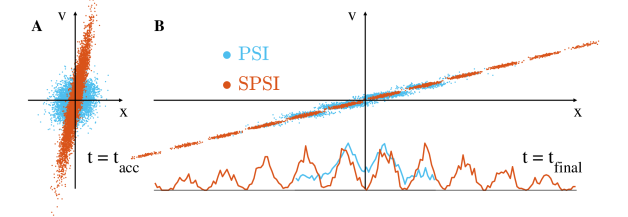
Figure 1: Principle of the squeezing effect in the interferometer. The atomic phase-space distribution is shown for the standard PSI interferometer (blue) and the SPSI interferometer (orange), at two different times: (A) at the start of the interferometer sequence, $t_{\rm{acc}}$, occurring just after the acceleration stage due to the repulsive-potential pulse, and (B) at the imaging time, $t_{\text{final}}$, following the complete interferometer sequence. The phase-space distribution at $t_{\rm{final}}$ becomes significantly tilted due to expansion, and the velocity-dependent interferometer phase introduces an oscillatory phase-space density upon detecting a single state. As shown at the bottom of (B), the latter oscillation produces a spatial density oscillation, which, upon being projected onto the position axis, forms the observed signal (output) of the interferometer. In the SPSI, when the initial phase-space distribution is squeezed with increased velocity, the subsequent expansion results in a phase-space distribution having a high aspect ratio. Upon projection onto the position axis, the SPSI signal shows significant improvement with more oscillations and an improved contrast.

Background

An established method for constructing a Laser-Pulse Atom Interferometry (LPAI) system involves a splitting a recombining laser giving rise to stimulated transitions (e.g., Raman, Bragg, or single photons for clock transitions) to implement a $\pi/2-\pi-\pi/2$ pulse sequence. The resulting phase shift (?), for free-falling atoms, is typically described by

$$\Delta\Phi=\mathbf{K}_{\text{eff}}\cdot\mathbf{a}{T_{R}}^{2}+2\mathbf{K}_{\text{eff}}\cdot\left(\mathbf{\Omega}\times\mathbf{v}\right){T_{R}}^{2},$$ (1)

where $\mathbf{K}_{\text{eff}}$ is the wave vector of the momentum given to the atom during the laser pulse, $\mathbf{a}$ is the constant acceleration of the platform relative to the atoms (including gravity), $T_{R}$ is the time interval between the interferometer pulses, $\mathbf{\Omega}$ represents the rotation of the platform, and $\mathbf{v}$ denotes the atom’s velocity. The second term in this equation is identified as the rotation phase. To effectively implement LPAI gyroscopes based on the $\pi/2-\pi-\pi/2$ pulse sequence, it is important to differentiate phase shifts induced by rotations from those caused by accelerations of the experimental apparatus. This can be achieved by combining the signals from two interferometers with counter-propagating atoms (?, ?, ?, ?).

The rotation phase in Eq. 1, can be expressed as the Sagnac phase (?) $\Delta\Phi_{\Omega}=(2m/\hbar)\mathbf{\Omega}\cdot\mathbf{A}$. In this context, $m$ is the atomic mass, while $\mathbf{A}$ is the area enclosed by the interferometer arms. Notably, these two expressions for the phase shift are equivalent, as demonstrated through the relation $\mathbf{A}=\left(\mathbf{v}_{r}T_{R}\right)\times\left(\mathbf{v}T_{R}\right)$, where $\mathbf{v}_{r}=\hbar\mathbf{K}_{\text{eff}}/m$ is the atom’s recoil velocity. Thus, the rotation measurement in LPAI gyroscopes depends on two distinct velocities: the recoil velocity and the axial velocity. The recoil velocity is linked to the momentum imparted on the atoms by the splitting and recombining laser. In the conventional Raman method, this momentum is equivalent to $2\hbar\mathbf{K}=\hbar\mathbf{K_{\text{eff}}}$, where $\mathbf{K}$ is the wave-vector of the Raman laser, although advanced techniques have demonstrated the potential to achieve significantly higher values  (?, ?, ?, ?, ?, ?, ?, ?, ?, ?, ?, ?, ?). The axial velocity is the topic of this work.

Results

Characteristics and Limits of PSI for Rotation Sensing

The point-source interferometer (PSI) is a specific kind of light-pulse atom interferometer in an expanding cloud of cold atoms  (?, ?, ?), and it is used in the following as a case study to examine in detail how the performance-enhancing phase-space squeezing works. The PSI method employs a single cloud of cold atoms and measures the rotation of the platform by probing the spatial frequency of the atomic density of a given output atomic state formed in the cloud. The method exploits the correlation between position and velocity generated by the expansion of the cloud throughout the interferometer sequence. When the final size of the cloud significantly exceeds its initial size, each atom’s final position, $\mathbf{x}$, is essentially dictated by its initial thermal velocity, $\mathbf{v}$. This allows for the approximation $\mathbf{x}\approx\mathbf{v}T_{\text{ex}}$, where $T_{\text{ex}}$ represents the total expansion time. In this limit, the Sagnac phase becomes  (?)

$$\Delta\Phi_{\Omega,\text{PS}}=\frac{2{T_{R}}^{2}}{T_{\text{ex}}}\left(\mathbf{K}_{\text{eff}}\times\mathbf{\Omega}\right)\cdot\mathbf{x}\equiv\mathbf{k}_{x}\cdot\mathbf{x}.$$ (2)

This phase is subsequently encoded as a spatial fringe pattern onto the image of the expanded cloud of atoms at the conclusion of the interferometer sequence. It is important to highlight that any deviation from the established position-velocity correlation results in a reduction of contrast within the fringe pattern, consequently diminishing the precision of the rotation measurement. Thus, to attain an approximation of a point source, it is necessary to cool and confine the atoms, resulting in reduced thermal velocities. However, this in turn leads to a smaller interferometer area, thus yielding lower resolution. Therefore, to enhance the resolution of the rotation phase measurement, it is advantageous to increase these velocities while preserving the position-velocity correlation.

According to Eq. 2, the probability of an atom with initial velocity $\mathbf{v}$ to be at the end of the interferometric sequence in a given internal state $|s\rangle$ is $P_{s}({\bf v})=1/2\cdot[1+\cos(\mathbf{k}_{v}\cdot\mathbf{v}+\phi_{s})]$, where $\mathbf{k}_{v}=2(\mathbf{K}_{\rm eff}\times\mathbf{\Omega})T_{R}^{2}$ and $\phi_{s}$ is determined by the gravitational acceleration. In an ideal case, the atomic cloud starts to expand freely from a point source, and the position of each atom is linearly proportional to its velocity $\mathbf{x}=\mathbf{v}T_{\rm{ex}}$, where $T_{\rm{ex}}$ is the time of expansion. In this case, the atoms form a spatial density that oscillates with a wave-vector $\mathbf{k}_{x}$, according to Eq. 2, from which one extracts the angular velocity component, which is transverse to the plane defined by the vectors $K_{\rm{eff}}$ and $k_{x}$.

In the more realistic case, we may consider an initial cloud with an isotropic Gaussian spatial distribution having a width $\sigma_{x0}$ and a Gaussian velocity distribution having a width $\sigma_{v0}$. In this case, one can show that the output density has the form  (?)

$$\rho({\bf x})\propto e^{-x^{2}/2\sigma_{f}^{2}}[1+C\cos(\alpha\mathbf{k}_{x}\cdot{\bf x}+\phi_{s})],$$ (3)

where $\sigma_{f}=\sqrt{\sigma_{x0}^{2}+T_{\rm{ex}}^{2}\sigma_{v0}}$ is the final cloud width, $\alpha=1-\sigma_{x0}^{2}/\sigma_{f}^{2}$, and the contrast $C$ is given by

$$C=\exp\left[-\frac{1}{2}k_{x}^{2}\sigma_{x0}^{2}\left(1-\frac{\sigma_{x0}^{2}}{\sigma_{f}^{2}}\right)\right]\,.$$ (4)

The sensitivity of an interferometer to rotation, limited by projection noise, hinges on two factors: the number of atoms per operation ($N$) and the frequency of operations ($\nu$). This sensitivity ($\delta\Omega$) is given by the expression  (?):

$$\delta\Omega=\frac{T_{\rm{ex}}/T_{R}^{2}}{2C\sqrt{N\nu/2}K_{\text{eff}}\sigma_{f}}\,,$$ (5)

where it is preferable to use a longer interferometer duration ($T_{R}$) and enlarge the cloud size ($\sigma_{f}$) to achieve good sensitivity.

In contrast to PSI, in interferometric rotation sensors, where the signal is atom population or light intensity in two output ports, the measured quantity is the Sagnac phase, which typically exhibits a linear correlation with the rotation. The smallest measurable phase difference determines the smallest detectable change in rotation, whether from zero rotation or from any given rotation. Hence, sensitivity characterizes both the smallest detectable rotation and the uncertainty in detecting a given rate of rotation. On the otherhand, in the PSI, the minimum detectable rotation by the interferometer is determined by the condition that the cloud size exceeds the period of spatial oscillation, expressed as $k_{x}\sigma_{f}>1$. In addition, the rotation should not surpass the threshold where the contrast significantly diminishes due to the ratio between the fringe periodicity and the initial cloud size, specified as $k_{x}\sigma_{x0}>1$. This implies a constraint on the fringe periodicity within the range $1/\sigma_{f}<k_{x}<1/\sigma_{x0}$, leading to a limitation on the dynamic range of the interferometer, namely, $\Omega_{\rm min}<\Omega<\Omega_{\rm max}$, where from Eq. 2 (and neglecting $\alpha$ from Eq. 3) we find

$$\Omega_{\rm min}\sim\frac{T_{\rm{ex}}/T_{R}^{2}}{2K_{\text{eff}}\sigma_{f}}\,,\quad\Omega_{\rm max}\sim\frac{T_{\rm{ex}}/T_{R}^{2}}{2K_{\text{eff}}\sigma_{x0}}\,,$$ (6)

such that $\Omega_{\rm max}/\Omega_{\rm min}\sim\sigma_{f}/\sigma_{x0}$. These limits are approximations closely related to the method used for image analysis. Previous works discussed this issue within various methods, including the ellipse fitting procedure  (?), phase shear  (?), or phase map  (?). Finally, it should be noted that by combining Eqs. 5 and 6, the sensitivity in detecting a rotation rate, $\delta\Omega$, is associated with the minimally detectable rate, $\Omega_{\rm{min}}$, by the relationship $\delta\Omega\approx 1/\sqrt{N/2}$. This suggests that for PSI, the sensitivity ($\delta\Omega$) solely pertains to uncertainty and may be significantly smaller (better) than the smallest detectable rotation rate.

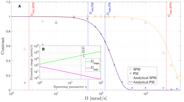
Figure 2: Contrast and dynamic range. (A) Contrast vs. angular velocity ($\Omega$). Using ⁸⁷Rb atoms, the simulation parameters are initial cloud size $\sigma_{x0}=100\,\rm{\mu m}$, temperature $T=5\,\rm{\mu K}$, and time between pulses $T_{R}=5\,\rm ms$. For the repulsive potential, we take a beam power of $P=1\,$W with a cross-section of $400\crossproduct 400\,\mu$m², blue-detuned by $\Delta=2\pi\cdot 10\,$GHz, and focused such that in the direction of acceleration it gives rise to an inverted harmonic potential and in the transverse direction a constant potential. The harmonic profile was optimized for achieving a large squeezing factor before the atoms exceed the region where the repulsive potential is harmonic. Following Eqs. 8 and 11, and choosing $t_{\text{acc}}=80.6\,\mu$s, we find a squeezing parameter of 22.81. The purple line represents the analytical solution of PSI contrast, while the dashed orange line corresponds to SPSI, according to Eq. 4. The data points are the result of a numerical simulation. While the contrast reduction due to the ratio between the fringe periodicity and the initial cloud size determines the upper limit of the detection range, there exists a lower limit when the fringe period becomes larger than the final cloud size. These limits are roughly given by $\Omega_{\rm min}$ and $\Omega_{\rm max}$ (Eq. 6), which are presented in the graph as vertical dashed lines. It is evident that using the SPSI improves the contrast significantly, thereby increasing the detection dynamic range. At high angular velocities, the contrast of the data points decreases faster than the analytical solution due to the short spacing between fringes relative to the detection pixel size considered only in the numerical calculation. (B) The analytical curve of the detection range as a function of $\eta$ according to Eq. 6. The dashed line presents the SPSI simulated in (A) with $\eta=22.81$.

Squeezed Point Source Interferometer

Integrating a repulsive potential that varies spatially to accelerate atom motion, either prior to or during the interferometer sequence, has the capability to substantially enhance the operational efficiency and sensitivity of a PSI device. Repulsive forces have been discussed in numerous contexts  (?, ?, ?, ?, ?, ?), but here, the repulsive potential has the role of enlarging the area enclosed by the interferometer arms, while maintaining and even improving the crucial position-velocity correlation. This is achieved by applying a repulsive potential for an acceleration time $t_{\rm acc}$. Let us define the coordinate system such that the $z$ axis is along the direction of the splitting and recombining laser beam. We may apply a quadratic repulsive potential along one or two axes transverse to $z$, but for the sake of simplicity, we describe only the dynamics along the $x$ coordinate. If the repulsive potential is quadratic $V_{\rm r}(x)=-(1/2)m\omega^{2}x^{2}$, where $m$ is the atomic mass, then after the acceleration stage, the initial coordinates in the direction $x$ of an atom are transformed as

$$x(t_{\rm acc})=c\cdot x(0)+s\cdot v_{x}(0)/\omega\,,\quad v_{x}(t_{\rm acc})=\omega s\cdot x(0)+c\cdot v_{x}(0)\,,$$ (7)

where $c=\cosh(\omega t_{\rm acc})$ and $s=\sinh(\omega t_{\rm acc})$.

It is easy to show that the phase-space distribution that forms after the repulsive pulse is exactly equivalent to the distribution that forms after free propagation for an effective duration $t_{\rm eff}$ when the initial distribution is squeezed with effective position uncertainty $\tilde{\sigma}_{x0}=\sigma_{x0}/\eta$ and velocity uncertainty $\tilde{\sigma}_{v0}=\eta\sigma_{v0}$, with the squeezing parameter being

$$\eta\equiv\sqrt{c^{2}+\frac{\omega^{2}\sigma_{x0}^{2}}{\sigma_{v0}^{2}}s^{2}},$$ (8)

and the effective time is given by

$$t_{\rm eff}=\frac{sc}{\omega\eta^{2}}\left(1+\frac{\omega^{2}\sigma_{x0}^{2}}{\sigma_{v0}^{2}}\right)\,.$$ (9)

If $\omega t_{\rm acc}\ll 1$ and $r\equiv\omega\sigma_{x0}/\sigma_{v0}\ll 1$ then $\eta\approx 1$ and $t_{\rm eff}\approx t_{\rm acc}$, such that the acceleration phase is ineffective. Conversely, if $\omega\gg\sigma_{v0}/\sigma_{x0}$ ($r\gg 1$) then even if the acceleration time is not long, such that $\omega t_{\rm acc}\lesssim 1$, then the squeezing parameter is large $\eta\sim r\omega t_{\rm acc}$ and the effective expansion time is $t_{\rm eff}\sim t_{\rm acc}/(\omega t_{\rm acc})^{2}$. If the acceleration time is long, such that $\omega t_{\rm acc}>1$ the squeezing becomes exponentially large such that $\eta\approx\sqrt{1+r^{2}}e^{\omega t_{\rm acc}}$ and $t_{\rm eff}\approx 1/\omega$ is inversely proportional to the repulsive frequency.

The repulsive potential can be generated by a laser beam blue-detuned from the atomic resonance by $\Delta>0$. The effective ac Stark-shift is  (?)

$$V_{\rm ac}(\mathbf{r})=\hbar\frac{\Omega_{R}(\mathbf{r})^{2}}{4\Delta}=\frac{3\pi\Gamma}{2k_{0}^{3}c}\frac{I(\mathbf{r})}{\Delta}\,,$$ (10)

where $\Omega_{R}$ is the local Rabi frequency, $k_{0}=2\pi/\lambda_{0}$ is the optical transition wave-vector, $\Gamma$ is the spontaneous emission rate, $I(\mathbf{r})$ is the light intensity, and $c$ is the speed of light. The inverse harmonic repulsive potential could be implemented by the quadratic intensity profile near the center of a Gaussian beam propagating along the $z$ direction. However, a more efficient acceleration may be achieved by designing a fully quadratic beam shape. Here we consider acceleration in the $x$ direction induced by a laser beam propagating along the $y$ direction and having a homogeneous profile in the $z$ direction in the volume containing the atom cloud. The light beam profile is $I(x,z)=I_{0}(1-x^{2}/x_{0}^{2})$ for $|x|<x_{0}$, $|z|<z_{0}/2$ and zero otherwise, where $I_{0}$ is the peak intensity and $2x_{0}z_{0}$ is the beam cross-section. The peak intensity equals $I_{0}=3P/4x_{0}z_{0}$, where $P$ is the beam power, and the potential frequency becomes

$$\omega_{\text{Harmonic}}=\sqrt{\frac{9\pi\Gamma P}{4mk_{0}^{3}c\Delta x_{0}^{3}z_{0}}}.$$ (11)

The harmonic profile is quite advantageous for achieving a significant squeezing factor before the atoms reach the region with a repulsive potential. For example, for the parameters introduced in Fig. 2, $\omega_{\text{Harmonic}}=2\pi\cdot 1220\,$Hz.

The optical repulsive potential has the consequent effect of heating the atoms due to scattered photons  (?). Along the direction of beam propagation, the atoms gain momentum in correlation to the spatial intensity $I(\textbf{r})$, which can be compensated by shifting the initial cloud or, if necessary, by employing a counter-propagating beam. In addition, the scattering induces a random walk in velocity space in all directions, potentially enlarging the effective initial cloud size, $\tilde{\sigma}_{x0}$, and consequently decreasing the upper detection limit $\Omega_{\text{max}}$ (Eq. 6). Under the limitations we have taken for the laser power and typical parameter values, this effect reduces $\Omega_{\text{max}}$, e.g., by $\sqrt{2}$ for the parameters of Fig. 2. This effect can be reduced to a negligible level by improving the beam parameters, for example, by equally increasing the beam power $P$ and the detuning $\Delta$. More details about the heating process can be found in the appendix. One could also explore using different types of potential, such as magnetic gradients, to mitigate heating.

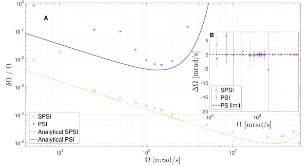
Figure 3: Relative sensitivity and measured angular velocity deviation. (A) Relative sensitivity $\delta\Omega/\Omega$ vs. $\Omega$, where $\Omega$ is the nominal (actual) angular velocity, for the same simulation parameters and notation as in Fig. 2. The analytical curves are determined according to Eq. 5. The data points for PSI are not shown at large angular velocities since $\delta\Omega/\Omega$ exceeds the value of 1, thus irrelevant. (B) Simulation results of the measured angular velocity deviation $\Delta\Omega\equiv(\Omega_{\rm meas}-\Omega)$ for different angular velocities. Here $\Delta\Omega$ denotes the discrepancy between the measured and nominal angular velocities, while the sensitivity (uncertainty) $\delta\Omega$ is represented by the error bars. The data point labels are the same as in (A), while the black dashed line illustrates the point-source (PS) limit of zero deviation. The data points for PSI are not shown at large angular velocities since $\Delta\Omega$ is too large. The enhanced performance of the SPSI in dynamic range, precision, and sensitivity (base noise) is clearly visible.

Performance Analysis

To estimate the performance of the SPSI and compare it to that of the standard PSI, we calculated its characteristics analytically and numerically (see Methods for the latter).

In Fig. 2(A), the fringe pattern’s contrast is plotted against the angular velocity for both methods. This illustrates that SPSI can measure higher angular velocities as its contrast diminishes at higher angular velocities, much larger than for standard PSI. We briefly note that at large angular velocities, the fringe spatial frequency becomes high and the detection pixel resolution becomes a limiting factor, causing the numerical contrast to decay more rapidly than the analytically predicted decay, which does not account for this limitation. Similarly, the SPSI can measure lower angular velocities than the PSI because its final cloud radius is larger, rendering it more sensitive to slow angular velocities characterized by low spatial fringe frequency. This improvement in both limits is depicted in Fig. 2(B) by the analytical curve of the detection range as a function of $\eta$ according to Eq. 6.

Fig. 3(A) presents a comparison of the relative sensitivity $\delta\Omega/\Omega$ between the two methods. It demonstrates an improvement of over one order of magnitude when both methods operate within their dynamic range $(60\lesssim\Omega\lesssim 200\,\rm{mrad/s})$, with a notably superior ratio beyond that range. Additionally, in Fig. 3(B), the plot of angular velocity deviation $\Delta\Omega=(\Omega_{\rm meas}-\Omega)$ provides further support for the aforementioned claims.

To demonstrate the advantage of the SPSI in the compactness of the interferometer, we define the dimensionless parameter $a_{t}=T_{R,SPSI}/T_{R,PSI}$, representing the reduction in the Ramsey time in a compact SPSI relative to a standard PSI ($a_{t}<1$). Such a reduction would also reduce the fall distance $h$ during the interferometer by $a_{t}^{2}$. Additionally, the final cloud’s radius scales as $\sigma_{f}\sim a_{t}T_{\rm{ex}}\sigma_{v0}\eta$. Consequently, the sensitivity per shot is given by:

$$\delta\Omega>\frac{1}{a_{t}T_{R}^{2}\cdot 2K_{\text{eff}}C\sqrt{N/2}\cdot a_{t}\sigma_{v0}\eta},$$ (12)

such that the sensitivity per shot ratios become $\delta\Omega_{SPSI}/\delta\Omega_{PSI}=(C_{PSI}/C_{SPSI})/(a_{t}^{2}\cdot\eta$). For the design of a rotation sensor, it would be necessary to compromise between sensitivity and compactness and to identify the optimal operational point based on the parameters $\eta$ and $a_{t}$. Fig. 4 illustrates the advantage in single shot sensitivity offered by the SPSI over the standard PSI for different parameter values. It is evident from the figure that the incorporation of a repulsive potential allows for a sensitivity enhancement of up to two orders of magnitude, while concurrently reducing the cycle time by a factor of approximately two, or alternatively, decreasing the cycle time by around tenfold without compromising sensitivity.

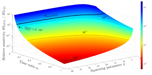
Figure 4: Sensitivity-compactness trade-off in the SPSI. The single shot sensitivity ratio $\delta\Omega_{SPSI}/\delta\Omega_{PSI}$ based on Eq. 12, is plotted against the squeezing parameter $\eta$ and the cycle time ratio $a_{t}=T_{SPSI}/T_{PSI}$ for an angular velocity of $\Omega=100\,\rm{mrad/s}$, while maintaining constant values for the remaining parameters: Time between pulses $T_{R}=10\,\rm{ms}$, temperature $T=2\,\rm{\mu K}$, and initial cloud size $\sigma_{x0}=100\,\rm{\mu m}$. The maximum value of $\eta$ was chosen to ensure that the majority of atoms are affected by the same potential throughout the acceleration phase. The bold black line indicates the validity boundary of this plot beyond which the minimal detectable angular velocity of the SPSI method (Eq. 13) exceeds the nominal angular velocity $\Omega$. It is evident that the implementation of a repulsive potential allows for a sensitivity enhancement of more than an order of magnitude, while simultaneously reducing the cycle time by a factor of about two (as indicated by the bright red color), or reducing the cycle time by approximately tenfold without affecting the sensitivity (as indicated by the light-blue color). Specifically, utilizing the compactness factor definition of Eq. 14, we find that with $\eta=40$ and $a_{t}=0.1$, we have a performance enhancement of $CF_{SPSI}/CF_{PSI}\simeq 2\cdot 10^{4}$ (black point).

Chip-Scale Device

Let us now compare between standard PSI and SPSI within the constraints of identical Ramsey times ($a_{t}=1$) and fall heights $h$ in the context of chip-scale devices. Employing the repulsive potential to expand acceleration parallel to the chip’s plane enables the SPSI method to optimize the device’s confinement.

For the comparison, under the same initial conditions (temperature, cloud size, and number of atoms), the ratio between the sensitivities obtained in the two methods is $\delta\Omega_{SPSI}/\delta\Omega_{PSI}\approx(C_{PSI}/C_{SPSI})/\eta$. Within the dynamic range of both methods, the contrast ratio is approximately $\sim 1$, while the detection limits ratio is $\Omega_{\rm min,SPSI}/\Omega_{\rm min,PSI}=1/\eta$ and $\Omega_{\rm max,SPSI}/\Omega_{\rm max,PSI}=\eta$. Consequently, for chip-scale devices, we can expect a sensitivity improvement of about $\eta$ and an increase in the dynamic range $\Omega_{\rm max}/\Omega_{\rm min}$ by a factor of $\eta^{2}$.

Specifically, we consider the following chip-scale scenario: a rectangular vacuum cell with dimensions of $1\,\rm{mm}\times 10\,\rm{mm}\times 10\,\rm{mm}$, with the short dimension aligned perpendicular to the direction of the repulsive potential’s acceleration. The SPSI sequence commences with the capture of an atomic cloud comprising $N=10^{6}$ ⁸⁷Rb atoms, with a radius of $\sigma_{x0}=100\,\rm{\mu m}$ and temperature of $T=2\,\rm{\mu K}$, using a magneto-optical trap and optical molasses setup. Employing a fully harmonic potential characterized by dimensions of $x_{0}=200\,\rm{\mu m}$ and $z_{0}=400\,\rm{\mu m}$, with total power of $P=1\,\rm{W}$ and an acceleration time of $t_{\rm acc}=0.1\,\rm{ms}$, yields a squeezing parameter $\eta=46.2$, potential frequency $\omega_{\text{Harmonic}}=2\pi\cdot 1220\,$Hz, and final velocity uncertainty $\tilde{\sigma}_{v0}=0.64\,$m/s. Following acceleration, the atoms undergo a Ramsey sequence with a time $T_{R}=2.5\,\rm{ms}$, resulting in a total fall height of $h=120\,\rm{\mu m}$. The final cloud dimensions are $\sigma_{f,z}=170\,\rm{\mu m}$ height and $\sigma_{f,x}=0.33\,\rm{cm}$ width. Without heating, a vacuum dimension of $0.5\,\rm{mm}$ would suffice, but if heating is not mitigated, a vacuum dimension of $1\,\rm{mm}$ would be required, or alternatively, one would have to take into account that a significant amount of atoms could not be recaptured for the next cycle, and reloading atoms from a source would be required.

With a number of operations per second of $\tau=100\,\rm{s^{-1}}$, the SPSI exhibits a sensitivity of $\delta\Omega=1\,\rm{\mu\rm{rad}/(s\cdot\sqrt{Hz})}$ and a one-shot sensitivity of $\delta\Omega=10\,\rm{\mu\rm{rad}/s}$. The minimum and maximum detectable angular velocities are $\Omega_{\rm min}=7.5\,\rm{mrad/s}$ and $\Omega_{\rm max}=11.47\,\rm{rad/s}$, respectively.

Studying the impact of heating due to the repulsive optical potential in a chip-scale device is crucial. The atoms acquire momentum in the direction of the optical repulsive potential beam, and this effect can be managed as discussed earlier. However, heating in the direction of the splitting and recombining laser beam presents more challenges, especially when we aim for the smallest possible chip. For the repulsive potential parameters outlined above, the calculation of the cloud’s final radius results in $\sigma_{z,f}\approx 300\,\mu\rm{m}$. This clearly remains within the defined $1\,\rm{mm}$ height limit. Additionally, as mentioned earlier, the dynamic range is restricted due to heating and is reduced in this example by a factor of approximately 3.

Discussion

Analysis of the simulation results from Fig. 4 reveals that employing squeezing can lead to a tenfold reduction in the cycle time without compromising sensitivity. Conversely, sensitivity enhancement by up to two orders of magnitude is achievable while concurrently reducing the cycle time by about two-fold. Considering that sensitivity per unit time scales as the inverse square root of the repetition rate $\nu_{\text{p}}=1/\tau_{\text{rep}}$, and noting that the relation between the repetition rates of SPSI and standard PSI scales as $a_{t}$, we derive $\delta\Omega_{SPSI}/\delta\Omega_{PSI}=(C_{PSI}/C_{SPSI})/a_{t}^{1.5}\cdot\eta$.

The ratios of the detection limits of PSI and SPSI are determined by:

$$\frac{\Omega_{\rm min,SPSI}}{\Omega_{\rm min,PSI}}=\frac{1}{a_{t}^{2}\cdot\eta},\quad\frac{\Omega_{\rm max,SPSI}}{\Omega_{\rm max,PSI}}=\frac{\eta}{a_{t}}.$$ (13)

Overall, the ratio $\Omega_{\rm max}/\Omega_{\rm min}$ changes by a factor of $\eta^{2}\cdot a_{t}$. Consequently, in the case of a tenfold reduction in the cycle time, the dynamic range would increase by more than two orders of magnitude.

To better quantify the performance improvement, we introduce a compactness factor

$$CF\equiv\frac{\Omega_{\text{max}}/\Omega_{\text{min}}}{\delta\Omega\cdot h}.$$ (14)

This factor encapsulates sensitivity $\delta\Omega$, dynamic range (as the ratio $\Omega_{\rm max}/\Omega_{\rm min}$, and the vertical size of the interferometer $h$. Based on the previous comparison between SPSI and PSI, we observe an improvement ratio of $\eta^{3}\cdot\sqrt{a_{t}}$, which can exceed four orders of magnitude. For instance, considering the conditions depicted in Fig. 4, with $\eta=40$ and $a_{t}=0.1$, we derive $CF_{\rm SPSI}/CF_{\rm PSI}\simeq 2\cdot 10^{4}$.

Finally, we note that details of the numerical analysis are presented in Materials and Methods, while the AC Stark interaction, heating by light and a full quantum approach are discussed in the appendices. As an outlook, let us note that accelerating the cloud expansion may also be realized by other interactions, such as repulsive magnetic forces or attractive electric forces. An accelerated expansion can even be acquired passively by diffracting a beam of atoms (e.g., from a 2D MOT) off a slit. An interesting problem left for future work is to find the optimal functional form of the repulsive potential.

To conclude, the SPSI described in this work enables either enhanced performance for standard size devices or maintaining the performance while miniaturizing to a chip-scale device, opening the door to real-life applications. It may very well be that the squeezed source presented here may be adapted to serve other types of matter-wave interferometers and quantum technology devices.

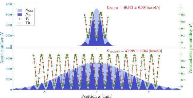
Figure 5: Simulation fringe pattern fit. This figure compares the simulation results of both methods, the top for PSI and the bottom for SPSI. The light blue shaded area depicts the total number of atoms in each bin, denoted as $N_{\text{total}}$, while the darker shade indicates only those atoms in the internal state $|1\rangle$, denoted as $N_{|1\rangle}$. The green points represent the normalized probability for the $|1\rangle$ state, calculated as $P_{1}=N_{|1\rangle}(x)/N_{\text{total}}(x)$, while the red line denotes the sinusoidal fit to these green points. The angular velocity is determined from the fit’s fringe spatial frequency using Eq. 3. The simulations begin with an initial 1D Gaussian cloud comprising $N=10^{6}$ atoms, with a width of $\sigma_{x0}=100\,\rm{\mu m}$ and a temperature of $T=5\,\rm{\mu K}$. For the PSI method, the atoms undergo free expansion during the interferometer sequence, with a time interval between pulses of $T_{R}=25\,\rm ms$, while the simulated angular velocity is $\Omega=40\,\rm{mrad/s}$. In the case of SPSI, the cloud is additionally subjected to a repulsive potential having a power of $P=1\,\rm{W}$, with a beam cross-section of $400\crossproduct 400\,\mu$m², activated for $t_{\text{acc}}=20\,\rm{\mu s}$. This results in a potential frequency of $\omega=2\pi\times 1.214\,\rm{kHz}$ (Eq. 11), a squeezing parameter $\eta=5.4$ (Eq. 8), and an effective time $t_{\text{eff}}=0.84\,\rm{ms}$ (Eq. 9). Consequently, the cloud size increases significantly. Note that the contrast and number of fringes in the PSI method is smaller than that of the SPSI (see Figs. 1-2), leading to a fit deviation and uncertainty one order of magnitude higher for the PSI case.

Materials and Methods

Numerical Analysis

To examine the impact of the SPSI, we conduct detailed numerical simulations for PSI and SPSI. Initially, we generate a cloud of $N$ atoms following the cooling phase, characterized by a spatial Gaussian distribution with a standard deviation of $\sigma_{x0}$. The atoms’ velocities follow a Maxwell-Boltzmann distribution corresponding to the given temperature. In a standard PSI simulation, the cloud undergoes expansion, followed by the initiation of the atomic-interferometer sequence with a time interval $T_{R}$ between pulses. Upon completion of this sequence, we determine the internal state of each atom using a Monte Carlo method. We simulate a two-state absorption of the atomic cloud by counting the atoms of each state in bins of spatial locations and normalizing the counts of one state to the total population in each bin $P_{1}=N_{|1\rangle}(x)/N_{\rm total}(x)$. This approach reveals the interferometer’s fringe pattern as per Eq. 2, illustrated in Fig. 5. Utilizing a sinusoidal fit allows us to extract the fringe’s periodicity, $k_{x}$, facilitating the calculation of angular velocity based on Eq. 3. The $\alpha$ factor is accounted for by scaling the fit’s frequency accordingly before extracting the angular velocity as described in Eq. 2. The uncertainty in angular velocity, denoted as single-shot sensitivity $\delta\Omega$, is computed based on the fit uncertainty. Running simulations for multiple repetitions and calculating the standard deviation provides a comparable result to the uncertainty derived from a single run’s fit.

In an SPSI simulation, we incorporate an additional stage: accelerating the atoms with a repulsive potential. We employ a blue-detuned inverted harmonic shaped light potential (Eq. 11) with a total power $P$ and beam dimensions $x_{0}$ and $z_{0}$, which accelerates the atoms over a brief duration of $t_{\rm acc}$. Following the acceleration stage, the simulation resumes in a manner identical to a standard PSI.

The normalized population is fitted to a sinusoidal function, $f(x)=A\sin(Bx+C)+D$, which initially employs an FFT algorithm to identify optimal frequencies and uses them as initial guesses for the fit algorithm, based on non-linear least-squares. To improve the fit’s success rate, we implement a basic image processing stage before normalizing $P_{1}$. This stage involves applying different averaging windows to the image’s pixels to reduce noise in the atom count in each bin. Additionally, the algorithm examines various windows of interest from the image, excluding the noisier edges where fewer atoms are counted and more significant fluctuations occur.

Acknowledgments
Funding: This work was partly supported by the Israel Science Foundation Grants No. 858/18, 1314/19 and 3515/20.

Repulsive potential by AC Stark shift

The preparation sequence for the atomic cloud begins with a 3D magneto-optical trap, followed by optical molasses to reduce the cloud’s temperature. Prior to applying the repulsive potential, we optically pump the ⁸⁷Rb atoms to the $|F=2,m_{F}=2\rangle$ atomic state. The repulsive potential is blue-detuned with circularly polarized $\sigma^{+}$ light, which ensures that any undesired excitation of the atoms decays back to the $|F=2,m_{F}=2\rangle$ state. The repulsive potential defines the quantization axis, eliminating the need for external magnetic fields. At the end of the acceleration and just before the interferometer sequence, we pump the atoms to the non-magnetic $|F=1,m_{F}=0\rangle$ state, so that the interferometric sequence may begin.

The blue-detuned light induces a positive-energy shift of the ground atomic level and a negative-energy shift of the excited level. As the energy shift is proportional to the light intensity, an atom in the ground level is repelled from the high-intensity beam center, while the excited level is drawn towards it. For the repulsion to be effective and to avoid heating by spontaneous emission, it is essential that $\Omega_{R}^{2}\ll\Delta^{2}$, so that the excited-level occupation stays small. For example, for the repulsive potential parameters used in Fig. 2, in the center of the potential ($I(x,z)=I_{0}$) we get $\Omega_{R}=2\pi\cdot 3.16\,\rm{GHz}$, such that $\Delta=2\pi\cdot 10\,\rm{GHz}$ gives a ratio of $\Delta^{2}/\Omega_{R}^{2}=10$.

An unavoidable effect of the repulsive potential is the heating of the atoms induced by scattered photons  (?). In the longitudinal direction of propagation of the light beam, the atoms experience an average heating of $4E_{\text{rec}}/3$ per scattering event, while in the two transverse directions, the heating amounts to $E_{\text{rec}}/3$ per scattering process, where $E_{\text{rec}}$ denotes the recoil energy, determining the recoil velocity $v_{\text{rec}}=\sqrt{2E_{\text{rec}}/m}$. Thus, the velocity increment in each axis for every scattering event equals $v_{\text{rec}}/\sqrt{3}$. The heating process along the acceleration direction contributes to an enlargement of the effective initial cloud’s spatial width, denoted as $\tilde{\sigma}_{x0,\text{eff}}=\sqrt{(\sigma_{x0}/\eta)^{2}+(t_{\text{eff}}\cdot\sigma_{v0,\text{heat}})^{2}}$, where $\sigma_{v0,\text{heat}}=\sqrt{N_{\text{sc}}/3}\cdot v_{\text{rec}}$ represents the heating due to the scattered photons from the repulsive potential. Here, $N_{\text{sc}}=\Gamma_{\text{sc}}t_{\text{acc}}$ signifies the number of scattering events, with $\Gamma_{\text{sc}}=(3\pi\Gamma^{2}I(\textbf{r}))/(2\hbar k_{0}^{3}c\Delta^{2})$ denoting the scattering rate. In the SPSI method, the effective reduction of $\sigma_{x0}$ augments $\Omega_{\text{max}}$, and this heating mechanism solely diminishes its value without compromising the sensitivity within the new detection range. If $(\sigma_{x0}/\eta)^{2}\gg(t_{\text{eff}}\cdot\sigma_{v0,\text{heat}})^{2}$, the effect of the scattering on the phase-space distribution becomes negligible. For the repulsive potential parameters used in Fig. 2, the relation is $(\sigma_{x0}/\eta)^{2}/(t_{\text{eff}}\cdot\sigma_{v0,\text{heat}})^{2}\approx 1$, and therefore in this example, heating only decreases $\Omega_{\text{max}}$ by a factor of $\approx\sqrt{2}$. A more detailed derivation will be provided in the following section.

The repulsive potential force in the direction of optical beam propagation adds a velocity in this axis equal to $v_{\text{long}}=N_{\text{sc}}v_{\text{rec}}$. Using the same potential and interferometer parameters as in Fig. 2, $v_{\text{long}}$ is equal to $28\,\rm{cm/s}$, resulting in a total longitudinal displacement of $\Delta x_{\text{long}}=2.8\,\rm{mm}$. This can be easily addressed by enlarging the vacuum cell or by setting the initial cloud away from the center of the cell.

Free evolution of a Gaussian phase-space distribution and the effect of heating

In a two-dimensional phase space, of position $x$ and velocity $v$, a Gaussian distribution in the form of an exponent of a bi-quadratic expression in $x$ and $v$ remains Gaussian in either free evolution or evolution in a quadratic potential. This conservation of the Gaussian form follows from the fact that any linear transformation of a bi-quadratic expression of two variables remains bi-quadratic under such a transformation. Any Gaussian form where the distribution is centered around $x=0$ and $v=0$ can be written in the form

$$\rho(x,v,t)\propto e^{-(x-vt)^{2}\sigma_{x0}^{2}}e^{-v^{2}/2\sigma_{v0}^{2}}\,,$$ (15)

which is a distribution that evolves under free propagation from an uncorrelated initial distribution at $t=0$ with a spatial uncertainty $\sigma_{x0}$ and velocity uncertainty $\sigma_{v0}$. This implies that any Gaussian distribution in phase space can be obtained by free propagation over an effective time $t_{\rm eff}$ starting from an uncorrelated distribution. This is the way that the effective squeezed distribution with a squeezing factor $\eta$ is obtained from the distribution that evolves under the repulsive inverse harmonic potential after acceleration over a time $t_{\rm acc}$. It is easy to acknowledge these properties by noting that a Gaussian distribution in phase space has an elliptical shape in the $x-v$ plane, and any ellipse can be transformed into an ellipse whose axes are aligned along the main axes by a proper rotation transformation.

The quadratic expression in the exponent can also be written in an alternative form that emphasizes the position-velocity correlations in the distribution:

$$\frac{(x-vt)^{2}}{2\sigma_{x0}^{2}}+\frac{v^{2}}{2\sigma_{v0}^{2}}=\frac{x^{2}}{2\sigma_{f}^{2}}+\frac{(v-x/T)^{2}}{2\sigma_{vt}^{2}}\,,$$ (16)

where $\sigma_{f}$ is the overall spatial width of the cloud, $\sigma_{vt}$ is the local velocity spread at any given point $x$ and $T$ is an effective time of evolution. The latter three parameters can be expressed in terms of the parameters $\sigma_{x0}$ and $\sigma_{v0}$ of the initial uncorrelated distribution and the time of evolution as

$$\sigma_{f}^{2}=\sigma_{x0}^{2}+\sigma_{v0}^{2}t^{2},\qquad\sigma_{vt}=\frac{\sigma_{x0}}{\sigma_{f}}\sigma_{v0}\,,\qquad T=t\left(1-\frac{\sigma_{x0}^{2}}{\sigma_{f}^{2}}\right)^{-1}.$$ (17)

The expression in Eq. 16 inside the exponent represents a distribution with correlation between position and velocity, such that at a given point $x$, the width of the velocity distribution is given by $\sigma_{vt}$, which is reduced relative to the initial uncertainty of the velocity by a factor representing the ratio between the initial cloud size and the final cloud size. It is evident that the phase-space volume is conserved during the evolution, as $\sigma_{f}\sigma_{vt}=\sigma_{x0}\sigma_{v0}$.

If, at a given time, a distribution has the form of Eq. 16, it is possible to express it as a distribution that started at a time $t$ before this time as an uncorrelated distribution of the form of Eq. 15. The variables $\sigma_{x0}$, $\sigma_{v0}$ and $t$ can then be expressed in terms of $\sigma_{f}$, $\sigma_{vt}$ and $T$. In particular, we find

$$\sigma_{x0}=\frac{\sigma_{vt}T}{\sqrt{1+\sigma_{vt}^{2}T^{2}/\sigma_{f}^{2}}}\,,$$ (18)

and the other two parameters are easily obtained from the latter.

Let us now consider a situation where an initial uncorrelated distribution has evolved in free space over a time $t_{\rm eff}$ and gave rise to a correlated distribution of the form of an exponent of Eq. 16 and then the width of the local velocity distribution $\sigma_{vt}$ has grown due to quick homogeneous heating. This means that after the heating, the parameters $\sigma_{f}$ and $T$ have remained the same as before the heating, while $\sigma_{vt}$ has grown due to heating. It is now possible to use Eq. 18 for determining the effective initial uncorrelated distribution that would have led by free propagation to the final distribution after heating.

If the heating is very strong, such that after the heating $\sigma_{vt}>\sigma_{f}$, then the projected initial cloud size at the starting point of the evolution is $\sigma_{x0,{\rm eff}}\approx\sigma_{f}$ and the subsequent evolution of the cloud will be similar to a cloud that starts with the final size of the cloud at the heating time. This means that the heating has erased the position-velocity correlation inside the cloud. Conversely, if the local velocity distribution has not grown considerably during the heating relative to the local velocity uncertainty without heating, then the effect of heating on the consequent evolution is negligible.

In the case of a squeezed phase-space distribution with squeezing factor $\eta\gg 1$ and a cloud size $\sigma_{f}$ after the acceleration that is not much larger than the real initial cloud, the local velocity uncertainty is given by $\sigma_{vt}=\eta\sigma_{v0}\cdot(\sigma_{x0}/\eta)/\sigma_{f}\sim\sigma_{v0}$, which is about the same as the real velocity uncertainty before the squeezing, while the effective initial velocity uncertainty is larger by a factor of $\eta$. Let us now assume that after the heating, the local velocity spread grows as $\sigma_{vt}\to\sigma_{vt,{\rm tot}}=\sqrt{\sigma_{vt,0}^{2}+\sigma_{v,h}^{2}}$, where $\sigma_{vt,0}$ is the local velocity spread before heating and $\sigma_{v,\rm{heat}}$ is the added spread due to heating. Considering the acceleration procedure and taking the free evolution time before heating to be $t_{\rm eff}$ and assuming $\sigma_{f}\gg\sigma_{x0,{\rm eff}}$, the effective initial cloud size projected back after heating becomes

$$\sigma_{x0,{\rm eff}}^{h}\approx\sigma_{vt,{\rm tot}}t_{\rm eff}=\sqrt{\sigma_{x0,0}^{2}+\sigma_{v,h}^{2}t_{\rm eff}^{2}}=\frac{\sigma_{vt,{\rm tot}}}{\sigma_{vt,0}}\sigma_{x0,0}\,,$$ (19)

where $\sigma_{x0,{\rm eff}}^{0}=\sigma_{x0}/\eta$ is the initial cloud size without heating and $\sigma_{x0,{\rm eff}}^{h}$ is the projected initial cloud size after heating. Here, we assumed that the ratio between the local velocity spread after heating and before heating is much smaller than the squeezing factor $\eta$.

Fully quantum derivation of a PSI - wave-packet approach

Consider an initial wave-function $\psi({\bf r})$ subject to a sequence of splitting and recombining pulses $\pi/2-\pi-\pi/2$ with an initial state $|0\rangle$ and another state $|1\rangle$. In the inertial frame, the initial pulse applies a momentum transfer $K_{\text{eff}}$ in the $\hat{z}$ direction to the state $|1\rangle$. The second pulse applies momentum kicks $\pm K_{\text{eff}}$ in a rotated direction $\cos\Omega T_{R}\hat{z}+\sin\Omega T_{R}\hat{x}$ to the two states, and the third pulse applies the positive momentum to the $|1\rangle$ state in the rotated direction $\cos 2\Omega T_{R}\hat{z}+\sin 2\Omega T_{R}\hat{x}$. When $\Omega T_{R}\ll 1$, we can ignore the effect of the rotation in the $\hat{z}$ direction, as $\cos\Omega T_{R}\approx 1$, and consider only the dynamics along the $\hat{x}$ direction, where we can approximate $\sin\Omega T_{R}\approx\Omega T_{R}$. Then the two paths end up in the same velocity but in different positions: The $|1\rangle-|0\rangle$ pulse ends up in $x=x_{0}+2v_{0}T_{R}-v_{R}\Omega T_{R}^{2}$ and the $|0\rangle-|1\rangle$ paths ends up in $x_{0}+2v_{0}T_{R}+v_{R}\Omega T_{R}^{2}$, where $v_{R}=\hbar K_{\text{eff}}/m$ is the recoil velocity. The phase difference between the two paths due to the velocity difference in the $x$-direction follows from the rotation

$$\delta\phi_{\rm rot}=\frac{m}{2\hbar}[(v_{0}-v_{R}\Omega T_{R})^{2}-(v_{0}+v_{R}\Omega T_{R})^{2}]T_{R}=-2K_{\text{eff}}v_{0}\Omega T_{R}^{2}.$$ (20)

The wave function in the state $|0\rangle$ after the sequence is then

$$\psi_{f}(x)=\frac{1}{\sqrt{2}}[\psi_{\sigma}(x-x_{a})+\psi_{\sigma}(x-x_{b})e^{-i\delta\phi_{\rm rot}}],$$ (21)

where $x_{a}$ and $x_{b}$ are the final positions of the two paths and $\psi_{\sigma}$ is the wave function after expansion from an initial width $\sigma_{0}$ to a final width $\sigma$ after a time $t=2T_{R}$. It follows that the final wave function is similar to the result of an expansion starting with two Gaussian wave-packets centered at a relative distance $d=|x_{a}-x_{b}|=2v_{R}\Omega T_{R}^{2}$, leading to the emergence of a fringe pattern in a manner equivalent to the double-slit experiment. Here, the distance $d$ is proportional to the square of the interferometer time, but the fringe periodicity depends on the total expansion time since the wave packet had a minimal size.

The evolution of a Gaussian wave-packet in free space, or alternatively a Bose-Einstein wave-packet in free space or a quadratic potential, can be expressed in terms of the evolution of the width $\sigma$. The simplified expression for one dimension in the frame moving with the center of the wave-packet is given by  (?, ?)

$$\psi_{\sigma}(x,t)=\frac{\psi_{0}[x/\lambda(t)]}{\sqrt{\lambda(t)}}\exp\left(\frac{im}{2\hbar}\frac{\dot{\sigma}}{\sigma}x^{2}\right)\,,$$ (22)

where $\psi_{0}(x)$ is the initial wave-packet wave function and $\lambda(t)=\sigma(t)/\sigma(0)$. The evolution of the width of a Gaussian wave-packet in free space is given by

$$\sigma(t)=\sqrt{\sigma(0)^{2}+\hbar^{2}t^{2}/4m^{2}\sigma(0)^{2}}=\sqrt{\sigma_{x0}^{2}+\sigma_{v0}^{2}t^{2}}\,,$$ (23)

with $\sigma_{v0}=\hbar/2m\sigma_{x0}$ for a coherent Gaussian wave-packet.

If we take, without loss of generality, $x_{0}=0$ and $v_{0}=0$ then the phase $\delta\phi_{\rm rot}=0$ and the phase difference between the two wave functions centered at $x_{a}$ and $x_{b}$ at a given point $x$ follows from the quadratic phases of the expanding Gaussians of the form of Eq. 22 and given by

$$\delta\phi(x)=\frac{m\dot{\sigma}}{2\hbar\sigma}[(x-v_{R}\Omega T_{R}^{2})^{2}-(x+v_{R}\Omega T_{R}^{2})^{2}]=-k_{\Omega}x,$$ (24)

where $k_{\Omega}=2(\dot{\sigma}/\sigma)K_{\text{eff}}\Omega T_{R}^{2}$.

For a Gaussian wave-packet with an initial width $\sigma_{0}$, the relative rate of expansion is given by

$$\frac{\dot{\sigma}}{\sigma}=\frac{\omega^{2}t}{1+\omega^{2}t^{2}}=\frac{1}{t}\left(1-\frac{\sigma_{x0}^{2}}{\sigma_{f}^{2}}\right)\,,$$ (25)

where $\omega=\hbar/2m\sigma(0)^{2}=\sigma_{v0}/\sigma_{x0}$. Therefore, we obtain the semi-classical result for expansion time of $t=T_{ex}$

$$k_{\Omega}=2K_{\text{eff}}\Omega\frac{T_{R}^{2}}{T_{ex}}\left(1-\frac{\sigma_{0}^{2}}{\sigma_{f}^{2}}\right).$$ (26)

In the limit of long times, where $\sigma_{f}\gg\sigma_{0}$, this becomes the well-known double-slit interference wave vector $k_{\Omega}=md/\hbar T_{ex}$. The contrast is obtained by observing the amplitude of the interference term

$$\exp\left[-\frac{(x-d/2)^{2}}{4\sigma_{f}^{2}}-\frac{(x+d/2)^{2}}{4\sigma_{f}^{2}}\right]=e^{-x^{2}/2\sigma_{f}^{2}}e^{-d^{2}/8\sigma_{f}^{2}}.$$ (27)

It follows that the contrast is

$$C=e^{-d^{2}/8\sigma_{f}^{2}}=\exp\left(-\frac{1}{2}k_{\Omega}^{2}\frac{\sigma_{0}^{2}}{1-\sigma_{0}^{2}/\sigma_{f}^{2}}\right).$$ (28)

A thermal cloud could be modeled as a mixture of states. For example, a thermal cloud in an initial harmonic trap is a mixture of Hermite-Gaussian states

$$\rho(x,x^{\prime})=\sum_{n}w_{n}\Phi_{n}(x)\Phi_{n}^{*}(x^{\prime}),$$ (29)

where $n$ is the number of nodes in the function and runs from $0$ to $\infty$ and $w_{n}\propto\exp(-n\hbar\omega/k_{B}T)$ are the weights (probabilities) of the states $|n\rangle$. It is clear that a thermal Boltzmann distribution yields a Gaussian spatial distribution $\sum_{n}w_{n}|\Phi_{n}(x)|^{2}\propto\exp(-x^{2}/2\sigma_{T}^{2})$ with $\sigma_{T}=\sqrt{k_{B}T/m\omega^{2}}$ in a harmonic trap. It follows that for a thermal distribution $\sigma_{0}$ in Eq. 28 can be replaced by the width of the thermal distribution to obtain the right expression for the contrast of an interferometer with a thermal cloud. This expression for the contrast is identical to the expression appearing in  (?).

References

- 1. M. Kasevich, S. Chu, Atomic interferometry using stimulated Raman transitions, Phys. Rev. Lett. 67, 181 (1991).
- 2. D. W. Keith, C. R. Ekstrom, Q. A. Turchette, D. E. Pritchard, An interferometer for atoms, Phys. Rev. Lett. 66, 2693 (1991).
- 3. O. Carnal, J. Mlynek, Young’s double-slit experiment with atoms: A simple atom interferometer, Phys. Rev. Lett. 66, 2689 (1991).
- 4. F. Riehle, T. Kisters, A. Witte, J. Helmcke, C. J. Bordé, Optical Ramsey spectroscopy in a rotating frame: Sagnac effect in a matter-wave interferometer, Phys. Rev. Lett. 67, 177 (1991).
- 5. A. D. Cronin, J. Schmiedmayer, D. E. Pritchard, Optics and interferometry with atoms and molecules, Rev. Mod. Phys. 81, 1051 (2009).
- 6. R. Anderson, H. R. Bilger, G. E. Stedman, “Sagnac” effect: A century of Earth-rotated interferometers, American Journal of Physics 62, 975 (1994).
- 7. C. L. Garrido Alzar, Compact chip-scale guided cold atom gyrometers for inertial navigation: Enabling technologies and design study, AVS Quantum Science 1, 014702 (2019).
- 8. D. Savoie, M. Altorio, B. Fang, L. A. Sidorenkov, R. Geiger, A. Landragin, Interleaved atom interferometry for high-sensitivity inertial measurements, Sci. Adv. 4, eaau7948 (2018).
- 9. R. Geiger, I. Dutta, D. Savoie, B. Fang, C. Guarrido Alzar, B. Venon, A. Landragin, Quantum Optics, A. J. Shields, J. Stuhler, eds. (SPIE, Brussels, Belgium, 2016), p. 4.
- 10. P. Gillot, O. Francis, A. Landragin, F. Pereira Dos Santos, S. Merlet, Stability comparison of two absolute gravimeters: optical versus atomic interferometers, Metrologia 51, L15 (2014).
- 11. A. Bertoldi, et al., AEDGE: Atomic experiment for dark matter and gravity exploration in space, Exp Astron 51, 1417 (2021).
- 12. A. Bassi, L. Cacciapuoti, S. Capozziello, S. Dell’Agnello, E. Diamanti, D. Giulini, L. Iess, P. Jetzer, S. K. Joshi, A. Landragin, C. L. Poncin-Lafitte, E. Rasel, A. Roura, C. Salomon, H. Ulbricht, A way forward for fundamental physics in space, npj Microgravity 8, 49 (2022).
- 13. E. R. Elliott, et al., Quantum gas mixtures and dual-species atom interferometry in space, Nature 623, 502 (2023).
- 14. S. Abend, et al., Technology roadmap for cold-atoms based quantum inertial sensor in space, AVS Quantum Science 5, 019201 (2023).
- 15. T. L. Gustavson, A. Landragin, M. A. Kasevich, Rotation sensing with a dual atom-interferometer Sagnac gyroscope, Class. Quantum Grav. 17, 2385 (2000).
- 16. D. S. Durfee, Y. K. Shaham, M. A. Kasevich, Long-Term Stability of an Area-Reversible Atom-Interferometer Sagnac Gyroscope, Phys. Rev. Lett. 97, 240801 (2006).
- 17. B. Canuel, F. Leduc, D. Holleville, A. Gauguet, J. Fils, A. Virdis, A. Clairon, N. Dimarcq, C. J. Bordé, A. Landragin, P. Bouyer, Six-Axis Inertial Sensor Using Cold-Atom Interferometry, Phys. Rev. Lett. 97, 010402 (2006).
- 18. A. Gauguet, B. Canuel, T. Lévèque, W. Chaibi, A. Landragin, Characterization and limits of a cold-atom Sagnac interferometer, Phys. Rev. A 80, 063604 (2009).
- 19. R. Stevenson, M. R. Hush, T. Bishop, I. Lesanovsky, T. Fernholz, Sagnac Interferometry with a Single Atomic Clock, Phys. Rev. Lett. 115, 163001 (2015).
- 20. R. Gautier, M. Guessoum, L. A. Sidorenkov, Q. Bouton, A. Landragin, R. Geiger, Accurate measurement of the Sagnac effect for matter waves, Science Advances 8, eabn8009 (2022).
- 21. C. Janvier, V. Ménoret, B. Desruelle, S. Merlet, A. Landragin, F. Pereira Dos Santos, Compact differential gravimeter at the quantum projection-noise limit, Phys. Rev. A 105, 022801 (2022).
- 22. Z.-W. Yao, S.-B. Lu, R.-B. Li, J. Luo, J. Wang, M.-S. Zhan, Calibration of atomic trajectories in a large-area dual-atom-interferometer gyroscope, Phys. Rev. A 97, 013620 (2018).
- 23. K. A. Krzyzanowska, J. Ferreras, C. Ryu, E. C. Samson, M. G. Boshier, Matter-wave analog of a fiber-optic gyroscope, Phys. Rev. A 108, 043305 (2023).
- 24. W. Jia, P. Yan, S. Wang, Y. Feng, A dual atomic interferometric inertial sensor utilizing transversely cooled atomic beams, 2024 IEEE International Symposium on Inertial Sensors and Systems (INERTIAL) pp. 1–4 (2024). Doi: 10.1109/INERTIAL60399.2024.10502115.
- 25. H. Ammann, N. Christensen, Delta Kick Cooling: A New Method for Cooling Atoms, Phys. Rev. Lett. 78, 2088 (1997).
- 26. T. Kovachy, J. M. Hogan, A. Sugarbaker, S. M. Dickerson, C. A. Donnelly, C. Overstreet, M. A. Kasevich, Matter Wave Lensing to Picokelvin Temperatures, Phys. Rev. Lett. 114, 143004 (2015).
- 27. T. Luan, Y. Li, X. Zhang, X. Chen, Realization of two-stage crossed beam cooling and the comparison with Delta-kick cooling in experiment, Review of Scientific Instruments 89, 123110 (2018).
- 28. L. Dupays, D. C. Spierings, A. M. Steinberg, A. Del Campo, Delta-kick cooling, time-optimal control of scale-invariant dynamics, and shortcuts to adiabaticity assisted by kicks, Phys. Rev. Research 3, 033261 (2021).
- 29. S. Pandey, H. Mas, G. Vasilakis, W. Von Klitzing, Atomtronic Matter-Wave Lensing, Phys. Rev. Lett. 126, 170402 (2021).
- 30. C. J. Bordé, Quantum Theory of Atom-Wave Beam Splitters and Application to Multidimensional Atomic Gravito-Inertial Sensors, General Relativity and Gravitation 36, 475 (2004).
- 31. A. Gauguet, T. E. Mehlstäubler, T. Lévèque, J. Le Gouët, W. Chaibi, B. Canuel, A. Clairon, F. P. Dos Santos, A. Landragin, Off-resonant Raman transition impact in an atom interferometer, Phys. Rev. A 78, 043615 (2008).
- 32. J. K. Stockton, K. Takase, M. A. Kasevich, Absolute Geodetic Rotation Measurement Using Atom Interferometry, Phys. Rev. Lett. 107, 133001 (2011).
- 33. P. Berg, S. Abend, G. Tackmann, C. Schubert, E. Giese, W. P. Schleich, F. A. Narducci, W. Ertmer, E. M. Rasel, Composite-Light-Pulse Technique for High-Precision Atom Interferometry, Phys. Rev. Lett. 114, 063002 (2015).
- 34. G. Sagnac, Effet tourbillonnaire optique. la circulation de l’éther lumineux dans un interférographe tournant, J. Phys. Theor. Appl. 4, 177 (1914).
- 35. J. M. McGuirk, M. J. Snadden, M. A. Kasevich, Large Area Light-Pulse Atom Interferometry, Phys. Rev. Lett. 85, 4498 (2000).
- 36. S.-w. Chiow, T. Kovachy, H.-C. Chien, M. A. Kasevich, 102 k Large Area Atom Interferometers, Phys. Rev. Lett. 107, 130403 (2011).
- 37. T. Kovachy, P. Asenbaum, C. Overstreet, C. A. Donnelly, S. M. Dickerson, A. Sugarbaker, J. M. Hogan, M. A. Kasevich, Quantum superposition at the half-metre scale, Nature 528, 530 (2015).
- 38. B. Plotkin-Swing, D. Gochnauer, K. E. McAlpine, E. S. Cooper, A. O. Jamison, S. Gupta, Three-Path Atom Interferometry with Large Momentum Separation, Phys. Rev. Lett. 121, 133201 (2018).
- 39. J. Rudolph, T. Wilkason, M. Nantel, H. Swan, C. M. Holland, Y. Jiang, B. E. Garber, S. P. Carman, J. M. Hogan, Large Momentum Transfer Clock Atom Interferometry on the 689 nm Intercombination Line of Strontium, Phys. Rev. Lett. 124, 083604 (2020).
- 40. R. H. Parker, C. Yu, W. Zhong, B. Estey, H. Müller, Measurement of the fine-structure constant as a test of the Standard Model, Science 360, 191 (2018).
- 41. M. Gebbe, J.-N. Siemß, M. Gersemann, H. Müntinga, S. Herrmann, C. Lämmerzahl, H. Ahlers, N. Gaaloul, C. Schubert, K. Hammerer, S. Abend, E. M. Rasel, Twin-lattice atom interferometry, Nat. Commun. 12, 2544 (2021).
- 42. J. Li, G. R. M. Da Silva, W. C. Huang, M. Fouda, J. Bonacum, T. Kovachy, S. M. Shahriar, High Sensitivity Multi-Axes Rotation Sensing Using Large Momentum Transfer Point Source Atom Interferometry, Atoms 9, 51 (2021).
- 43. B. Dubetsky, Sequential large momentum transfer exploiting rectangular Raman pulses, Phys. Rev. A 108, 063308 (2023).
- 44. J.-N. Siemß, F. Fitzek, C. Schubert, E. M. Rasel, N. Gaaloul, K. Hammerer, Large-momentum-transfer atom interferometers with rad-accuracy using Bragg diffraction, Phys. Rev. Lett. 131, 033602 (2023).
- 45. M. H. Goerz, M. A. Kasevich, V. S. Malinovsky, Robust Optimized Pulse Schemes for Atomic Fountain Interferometry, Atoms 11, 36 (2023).
- 46. J. Li, G. R. M. Da Silva, S. Kain, J. Bonacum, D. D. Smith, T. Kovachy, S. M. Shahriar, Spin-squeezing-enhanced dual-species atom interferometric accelerometer employing large momentum transfer for precision test of the equivalence principle, Phys. Rev. D 108, 024011 (2023).
- 47. G. Louie, Z. Chen, T. Deshpande, T. Kovachy, Robust atom optics for Bragg atom interferometry, New J. Phys. 25, 083017 (2023).
- 48. S. M. Dickerson, J. M. Hogan, A. Sugarbaker, D. M. S. Johnson, M. A. Kasevich, Multiaxis Inertial Sensing with Long-Time Point Source Atom Interferometry, Phys. Rev. Lett. 111, 083001 (2013).
- 49. Y.-J. Chen, A. Hansen, G. W. Hoth, E. Ivanov, B. Pelle, J. Kitching, E. A. Donley, Single-Source Multiaxis Cold-Atom Interferometer in a Centimeter-Scale Cell, Phys. Rev. Applied 12, 014019 (2019).
- 50. D. Yankelev, C. Avinadav, N. Davidson, O. Firstenberg, Atom interferometry with thousand-fold increase in dynamic range, Sci. Adv. 6, eabd0650 (2020).
- 51. G. W. Hoth, B. Pelle, J. Kitching, E. A. Donley, Slow Light, Fast Light, and Opto-Atomic Precision Metrology X, S. M. Shahriar, J. Scheuer, eds. (SPIE, 2017), vol. 10119, p. 1011908.
- 52. J. Li, T. Kovachy, J. Bonacum, S. M. Shahriar, Quantum Sensing, Imaging, and Precision Metrology II, S. M. Shahriar, J. Scheuer, eds. (SPIE, 2024), p. 76.
- 53. G. T. Foster, J. B. Fixler, J. M. McGuirk, M. A. Kasevich, Method of phase extraction between coupled atom interferometers using ellipse-specific fitting, Opt. Lett. 27, 951 (2002).
- 54. A. Sugarbaker, S. M. Dickerson, J. M. Hogan, D. M. S. Johnson, M. A. Kasevich, Enhanced Atom Interferometer Readout through the Application of Phase Shear, Phys. Rev. Lett. 111, 113002 (2013).
- 55. Y.-J. Chen, A. Hansen, M. Shuker, R. Boudot, J. Kitching, E. A. Donley, Robust inertial sensing with point-source atom interferometry for interferograms spanning a partial period, Opt. Express 28, 34516 (2020).
- 56. O. Romero-Isart, Coherent inflation for large quantum superpositions of levitated microspheres, New J. Phys. 19, 123029 (2017).
- 57. C. Yuce, Quantum inverted harmonic potential, Phys. Scr. 96, 105006 (2021).
- 58. T. Weiss, M. Roda-Llordes, E. Torrontegui, M. Aspelmeyer, O. Romero-Isart, Large Quantum Delocalization of a Levitated Nanoparticle Using Optimal Control: Applications for Force Sensing and Entangling via Weak Forces, Phys. Rev. Lett. 127, 023601 (2021).
- 59. F. Ullinger, M. Zimmermann, W. P. Schleich, The logarithmic phase singularity in the inverted harmonic oscillator, AVS Quantum Science 4, 024402 (2022).
- 60. L. Neumeier, M. A. Ciampini, O. Romero-Isart, M. Aspelmeyer, N. Kiesel, Fast quantum interference of a nanoparticle via optical potential control, Proc. Natl. Acad. Sci. U.S.A. 121 (2024).
- 61. G. G. Rozenman, F. Ullinger, M. Zimmermann, M. A. Efremov, L. Shemer, W. P. Schleich, A. Arie, Observation of a phase space horizon with surface gravity water waves, Commun Phys 7, 165 (2024).
- 62. R. Grimm, M. Weidemüller, Y. B. Ovchinnikov, Advances In Atomic, Molecular, and Optical Physics (Elsevier, 2000), vol. 42, pp. 95–170.
- 63. Y. Castin, R. Dum, Bose-Einstein Condensates in Time Dependent Traps, Phys. Rev. Lett. 77, 5315 (1996).
- 64. Y. Japha, Unified model of matter-wave-packet evolution and application to spatial coherence of atom interferometers, Phys. Rev. A 104, 053310 (2021).
- 65. D. E. Miller, J. R. Anglin, J. R. Abo-Shaeer, K. Xu, J. K. Chin, W. Ketterle, High-contrast interference in a thermal cloud of atoms, Phys. Rev. A 71, 043615 (2005).