Remote control system of
a binary tree of switches –
I. constraints and inequalities

Abstract

We study a tree coloring model introduced by Guidon (2018), initially based on an analogy with a remote control system of a rail yard, seen as a switch tree. For a given rooted tree, we formalize the constraints on the coloring, in particular on the minimum number of colors, and on the distribution of the nodes among colors. We show that the sequence $(a_{1},a_{2},a_{3},\cdots)$, where $a_{i}$ denotes the number of nodes with color $i$, satisfies a set of inequalities which only involve the sequence $(n_{0},n_{1},n_{2},\cdots)$ where $n_{i}$ denotes the number of nodes with height $i$. By coloring the nodes according to their depth, we deduce that these inequalities also apply to the sequence $(d_{0},d_{1},d_{2},\cdots)$ where $d_{i}$ denotes the number of nodes with depth $i$.

1 Introduction

Since the appearance of computers, the notion of tree is central in computer sciences. For example to decompose program lines, the first Fortran compilers used a binary tree optimized for keyword recognition time. Tree structures are intensively used for databases, algorithms, representation of expressions in symbolic programming languages, etc.

Many variants have been developed to minimize searching time or to save memory, like B-tree and red–black tree. Trees are essential for network design and parallel computing: many computer clusters have a fat-tree network and algorithm performances depend on lengths of communication links between computer nodes.

The mathematician and computer scientist D.  Knuth, also creator of the TeX typesetting system, devotes a hundred pages to trees in his encyclopedia, The art of computer programming, and summarizes their development since 1847 [1, page 406].

Moreover coloring problems are frequent in graph theory. The most common rule for coloring a graph is that two adjacent vertices do not have the same color. Unfortunately this rule has little interest for a tree, which is a graph without loop: just alternate two colors along each branch.

By leafing through a general public review on Linux, we read an article [2] that describes how to control a binary tree of electronic switches with a minimum number of signals. The author Y. Guidon explains how to balance the signal power to avoid the bad situation where a single signal controls half of the switches. For that, he describes this problem in terms of binary tree coloring, but with a rule different from that usual in graph theory. He draws balanced solutions [2, 3] for perfect binary trees with height up to 5.

Our paper is devoted to this kind of coloring. In Section 2, we recall some usual definitions on trees. As Ref. [2] is in French and difficult to access for non-subscribers, we recall its analogy with a rail yard in Section 3 and its coloring rule in Section 4. In Section 5, we study the constraints to distribute the nodes of a given tree among the colors, according to their distribution by height in the tree. In Section 6, we give proofs of the inequalities stated on Section 5.

2 Definitions

To fix terminology, we quickly give some definitions. Most of them are common, but some differ according to the authors, like binary, full binary and perfect binary trees.

A graph is defined by a set of nodes (or vertices) and a set of edges (or links), where an edge is a pair of nodes. A tree is a connected graph without cycle. The size of a tree is the number of its nodes.

A rooted tree is a tree with a marked node, called the root; edges are now oriented away from the root. A rooted tree can be described as a family chart, with a common ancestor and the descendants. By convention, the root is drawn at the top, unlike real trees in nature.

The depth of a node $v$ is the number of edges between $v$ and the root. Only the root has depth $0$. A node with depth $d$ can share an edge with a child, a node with depth $d+1$, or a parent, a node with depth $d-1$.

Each node has only one parent, except the root without parent. Considering the number of children, there are two kinds of nodes: leaves with no children, and internal nodes with at least one child.

A sibling of a node $v$ is a node $w$ that has same parent as $v$, with $w\neq v$. A descendant is a child, or a descendant of a child; an ancestor is a parent, or an ancestor of a parent (recursive definitions).

The height of a node $v$ is the maximal distance between $v$ and the leaves among its descendants; leaves have height 0. The height of an internal node is $1+\max(\{h_{c}\})$, where the $h_{c}$’s are the heights of its children.

The height of a rooted tree is the height of its root; it is also the greatest depth of its leaves.

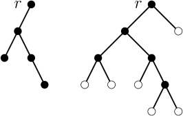
Figure 1: Left: a binary tree with root $r$ and $n=5$ nodes. Right: a full binary tree with $2n+1=11$ nodes ($n=5$ internal nodes in black and $n+1=6$ leaves in white). These two trees are in bijection by adding or removing white nodes; see text.

A binary tree is a kind of rooted tree where each node has at most 2 children, distinguishing left child and right child, even when there is only one child. In other words, each node has 0 or 1 left child, and 0 or 1 right child. For example, see Fig. 1.

A full binary tree is a binary tree where each node has 0 or 2 children. For example, see Fig. 1. A full binary tree with $n$ internal nodes has $n+1$ leaves, so $2n+1$ nodes.

There is a bijection [4, page 16] between the set $\mathcal{F}_{n}$ of full binary trees with $2n+1$ nodes and the set $\mathcal{B}_{n}$ of binary trees with $n$ nodes. Let $T_{F}\in\mathcal{F}_{n}$; this bijection consists in removing all the $n+1$ leaves of $T_{F}$ and keeping the skeleton made of the $n$ internal nodes: It is a binary tree $T_{B}\in\mathcal{B}_{n}$; see Fig. 1.

Starting with $T_{B}\in\mathcal{B}_{n}$, the reverse bijection consists in completing with leaves each node of $T_{B}$ that has less than two children. The new tree $T_{F}\in\mathcal{F}_{n}$ and its $n$ internal nodes are the nodes of $T_{B}$.

Consequently there are as many trees in $\mathcal{F}_{n}$ as in $\mathcal{B}_{n}$. It is a classical exercise to show that they are counted by Catalan numbers, $C_{n}=(2n)!/(n+1)!/n!$, sequence A000108 in OEIS [5]. A book [4] of R. P. Stanley presents 212 other kinds of object that are counted using Catalan numbers.

A perfect binary tree is a full binary tree in which all the leaves have same depth. All the perfect binary trees with a given height $h$ are isomorphic: Such a tree has $2^{d}$ nodes with depth $d$ and height $h-d$ for $0\leq d\leq h$, then $2^{h}-1$ internal nodes and $2^{h}$ leaves, so $2^{h+1}-1$ nodes. By removing the leaves, the sub-tree made of its internal nodes is a perfect binary tree with height $h-1$. Fig. 3 represents the perfect binary tree with height 2.

Among all the (full or not) binary trees, perfect binary trees are the most compact: Given a height $h$, a binary but not perfect tree has less than $2^{h+1}-1$ nodes.

3 Analogy with a rail yard

In this section, we follow the analogy made by Guidon [2, 3], between a full binary tree and a rail yard. Internal nodes are switches. Cars enter the tree through the root which is the first switch; then they are directed to leaves, which are exit tracks.

In a full binary tree, each switch has one input (parent) and two outputs (children). Each switch can be oriented to the right or left. The purpose of a rail yard is to choose an exit track, i.e. a leaf $v$, and to bring a car from the root $r$ to $v$. For that, it is necessary to orient correctly the switches along the path from $r$ to $v$, i.e. the ancestors of $v$. Generalization to all rooted trees is possible, by using switches with a variable number of outputs.

To easily operate a rail yard, it is convenient to control the switches remotely: We can send a binary signal $b_{u}$ to each switch $u$, for example $b_{u}=0$ for left or 1 for right. Consequently for a leaf $v$ with depth $d$, we need to send $d$ signals to the $d$ switches which are the ancestors of $v$. But we must be able to select all leaves, then to control all switches. Notice that leaves are passive and do not receive signal.

For a rail yard made up of $n$ switches, the maximum solution is to have a remote control system with $n$ signals, where each signal activates one and only one switch. In contrast, Guidon [2] asks the question of decreasing or even minimizing the number of signals. For practical examples (rail yard, electronic circuit, etc.), this may have an economic justification, to simplify the control system and reduce its cost.

For that, some signals must control more than one switch. But there are constraints: For each leaf $v$ with depth $d$, its $d$ ancestors must be controlled by $d$ independent signals. Since these signals can only take two values, left=0 or right=1, there will be pairs $\{u,w\}$ of ancestors of $v$ with signals of the same value, $b_{u}=b_{w}$. However, these two signals must remain independent, to be able to access other leaves, especially those that also have $u$ and $w$ as ancestors but with $b_{u}\neq b_{w}$. In other words, the same signal can control several switches provided there are no ancestor-descendant pairs among these switches.

4 Colored rooted trees

4.1 Coloring rule

From now on, we use coloring terminology by assigning a different label, called color, for each signal [2]. The problem now is to color all the internal nodes of a full binary tree with the following constraint: For each leaf, its ancestors must all be of different colors.

Note that the leaves are not colored; so we remove them. As explained in Section 2, this operation is a bijection that transforms a full binary tree $T_{F}$ with $n$ colored internal nodes into a binary tree $T_{B}$ with $n$ colored nodes (internal or leaves).

By definition, each node of a binary tree has at most two children, distinguishing left child and right child. This distinction is important in the analogy with a rail yard, but we can ignore it when we formulate the problem as a colored tree. We can also remove the constraint of having at most two children per node. So we can therefore generalize to all rooted trees.

Our problem is now reformulated as follows: color all the nodes of a rooted tree with the following rule: For each leaf $v$, $v$ and its ancestors must all be of different color. This is equivalent to the:

Coloring rule: For each pair of nodes $\{u,v\}$, if $u$ is an ancestor of $v$, they do not have the same color.

We remark that this constraint is stronger than the usual rule for graph coloring, such that two connected nodes do not have the same color.

As for graph coloring theory, values of color label do not matter. We can change or permute the labels without effects. Only counts the partition of the tree into subsets of nodes having the same color: Two colorings are equivalent if they give the same subsets of nodes.

4.2 Minimum number of colors

For a rooted tree of $n$ nodes, the maximum solution indicated above Section 3 corresponds to the maximum number $n$ of colors: one color per node. But we are rather interested in $\chi$, the minimum number of colors, which would be the equivalent of chromatic number in graph theory.

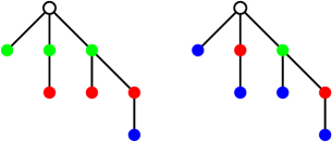
Figure 2: Left: Canonical coloring by depth. Right: Canonical coloring by height with blue, red, green and white for nodes with height 0, 1, 2 and 3.

For a rooted tree with height $h$, Guidon [2] shows that $\chi=h+1$. Indeed according to the definition of $h$, the maximum depth of a leaf is $h$; therefore $h+1$ different colors are already required for a leaf with depth $h$ and its $h$ ancestors. Consequently $\chi\geq h+1$. To prove equality, it remains to show a solution with $h+1$ colors. We will give two examples of minimum solutions in Fig. 2.

The first minimum solution is the canonical coloring by depth, where all nodes with depth $d$ have the same color $d+1$, for $0\leq d\leq h$. The second one is the canonical coloring by height, where all nodes with height $g$ have the same color $g+1$, for $0\leq g\leq h$.

Note that for a perfect binary tree, both canonical colorings, by depth or by height, are equivalent; indeed, all the nodes with depth $d$ have the same height, $g=h-d$.

4.3 Balancing of the nodes among colors

Guidon [2] asks a more difficult question: For a given tree, how to best balance the nodes among all the colors? Again the justification can be economical: If a signal controls many switches (or electrical relays), its circuit must have a high pneumatic (or electrical) power. It may also be slow because of the inertia of the switches. Also, we may be interested in a more balanced distribution to minimize total cost, or reaction times.

Let $T$ be a rooted tree with $n$ nodes, height $h$, and colored with the minimum number $\chi=h+1$ of colors indexed by $i=1,2,..,\chi$. Let $a_{i}$ be the number of nodes with color $i$. In our problem, $T$ is fixed: Work optimization relates only to $A=(a_{1},a_{2},\cdots,a_{\chi})$, i.e. the way to color $T$, but without modifying edges of $T$.

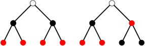
Figure 3: The two possible colorings with 3 colors for the perfect binary tree of height 2.

For example, for a perfect binary tree with height $h$ and $2^{h+1}-1$ nodes, the canonical coloring (by depth or equivalently by height) gives the distribution $A=(2^{h},\cdots,4,2,1)$ where more than half of the nodes have the same color. We will see that it is the maximally unbalanced coloring. But we can color it differently. For example, for a perfect binary tree with height 2, there are two possible colorings with $\chi=3$ colors, drawn in Fig. 3: the canonical coloring $A=(4,2,1)$ and another coloring $A^{\prime}=(3,3,1)$, better balanced [2].

For perfect binary trees, Guidon [2] offers a solution and an algorithm to minimize $\max_{i}(a_{i})$, equivalent to the maximum power of control signals. But we could also choose to minimize another quantity, for example, $\sum_{i}a_{i}^{2}$, or more generally the $p$’th moment $\mu_{p}=\sum_{i}a_{i}^{p}$. Note that the maximum corresponds to the limit $p\to\infty$. We may also want to maximize the coloring entropy $S=-\sum_{i}a_{i}\log(a_{i})$, knowing that $S=-\left.d\mu_{p}/dp\right|_{p=1}$. If we know the cost function $f(a_{i})$ of a circuit which controls $a_{i}$ switches, we will try to minimize the total cost $\sum_{i}f(a_{i})$.

5 Colorable partitions

We say that the non-negative integer sequence $A=(a_{1},a_{2},...,a_{c})$ is a colorable partition of a rooted tree $T$ if there exists a coloring of $T$ with $c$ colors where $a_{i}$ is the number of nodes of $T$ with color $i$ for $1\leq i\leq c$. In this section, we will study the conditions that the coloring partitions must satisfy.

To simplify the proof presented Section 6, we allow more colors than the minimum, so $c\geq\chi=h+1$ where $h$ denotes the height of $T$. Moreover we allow colors which do not color any nodes, i.e. with $a_{i}=0$. Note that this allows to have a number $c=\infty$ of colors, then $c$ is no longer a relevant parameter.

5.1 Necessary conditions

Let $T$ be a rooted tree with $n$ nodes, $h$ the height of $T$, and $n_{g}$ the number of nodes of $T$ with height $g$ for $g\geq 0$. If $A=(a_{1},a_{2},...,a_{c})$ is a colorable partition of $T$, then $A$ must satisfy the following conditions:

$$\sum_{i=1}^{c}a_{i}=n,$$ (1)

$$a_{i}=1\ \ \ \ \mbox{ for at least one color }i\ \ (1\leq i\leq c),$$ (2)

$$a_{i}\leq n_{0}\ \ \ \ (1\leq i\leq c),$$ (3)

$$a_{i}+a_{j}\leq n_{0}+n_{1}\ \ \ \ (1\leq i<j\leq c),$$ (4)

and more generally, for any subset of $k$ different colors $1\leq i_{1}<i_{2}<\cdots<i_{k}\leq c$ with $1\leq k\leq c$,

$$a_{i_{1}}+a_{i_{2}}\cdots+a_{i_{k}}\leq n_{0}+n_{1}\cdots+n_{k-1}.$$ (5)

Inequalities (3–5) are equivalent to

$$\max_{1\leq i\leq c}(a_{i}) \leq n_{0},$$ (6)

$$\max_{1\leq i<j\leq c}(a_{i}+a_{j}) \leq n_{0}+n_{1},$$ (7)

and more generally, for $1\leq k\leq c$,

$$\max_{1\leq i_{1}<i_{2}<\cdots<i_{k}\leq c}(a_{i_{1}}+a_{i_{2}}\cdots+a_{i_{k}})\leq n_{0}+n_{1}\cdots+n_{k-1}.$$ (8)

In general, these are necessary but not sufficient conditions. In Section 5.4, we will give examples of rooted, binary and full binary trees with sequences which satisfy these conditions but which do not correspond to any possible coloring.

Before proving these conditions in Section 6, we discuss first some of their consequences.

5.2 Canonical coloring by height

We first note that the sequence $(n_{0},n_{1}\cdots)$ satisfies $\sum_{i}n_{i}=n$, the total number of nodes; it is also monotonically decreasing (non-increasing). Indeed, for every $i\geq 0$, each internal node with height $i+1$ has at least one child with height $i$. Moreover each node with height $i$ (except the root) has a single parent, which can be height $i+1$ or greater. Consequently $n_{i}\geq n_{i+1}$. Note that $n_{i}=0$ if $i>h$, because $h$ is the maximum height of nodes of $T$, by definition.

In Section 4.2, we described the canonical coloring by height where all the nodes with the same height have the same color. So the sequence $(n_{0},n_{1},n_{2},\cdots)$ is therefore a colorable partition of $T$: it satisfies the above conditions with $a_{i}=n_{i-1}$. But here moreover, inequalities (6–8) become equalities.

As the $n_{i}$’s are monotonically decreasing, the colorable partition $(n_{0},n_{1},n_{2},\cdots)$ is the largest in lexicographical order among all the colorable partitions of $T$. In this sense, we can say that the canonical coloring by height is maximally unbalanced.

The inequality (6) gives a procedure to maximize the use of a color: color all leaves of $T$ with this color.

If we want to maximize $k$ colors one after the other, just color with the color $i$ the nodes with height $i-1$ for $1\leq i\leq k$.

To maximize $k$ colors overall, following inequality (8), just color with these $k$ colors all the nodes of the first $k$ levels, i.e. the nodes with height $i<k$; we can mix colors by levels, according to the different branches of the tree, but always respecting the coloring rule.

5.3 Canonical coloring by depth

Thanks to the inequalities (3–8), we obtain a non trivial relation between the distribution of the nodes by depth and their distribution by height.

Let $d_{i}$ be the number of nodes of $T$ with depth $i$. In Section 4.2, we described the canonical coloring by depth where all the nodes with the same depth have the same color. So $D=(d_{0},d_{1},d_{2},\cdots)$ is a colorable partition of $T$. Generally, the sequence $D$ is not necessarily increasing or decreasing. However, $D$ satisfies the inequalities (3–8) with $a_{i}=d_{i-1}$.

For example, the tree displayed in Fig. 2 has a distribution by depth $D=(1,3,3,1)$ and a distribution by height $(n_{0},n_{1},n_{2},n_{3})=(4,2,1,1)$. For this tree, Eq. (6) gives $3\leq 4$, Eq. (7) gives $3+3\leq 4+2$, Eq. (8) gives $3+3+1\leq 4+2+1$ for $k=3$, and $3+3+1+1\leq 4+2+1+1$ for $k=4$.

5.4 Necessary but not sufficient conditions

We prove in Section 6 that Eqs. (1–5) are necessary conditions, in other words if $A$ is a colorable partition of a rooted tree, then $A$ satisfies these equations.

We can easily draw trees for which these conditions are necessary and sufficient, but this is not generally true. There are trees $T$ for which these conditions are not sufficient, i.e. there is at least one sequence $A=(a_{1},a_{2},a_{3},\cdots)$ which satisfies these conditions but which do not correspond to any possible coloring of $T$ such that $a_{i}$ counts the nodes colored by $i$. We will give some examples of trees with non-sufficient conditions (TNSC).

Figure 4: The smallest rooted tree (left) and binary tree (right) with non-sufficient conditions.

The tree $T_{R}$ drawn in Fig. 4 is the smallest TNSC among rooted trees. It has $n=5$, $h=2$, and $(n_{0},n_{1},n_{2})=(3,1,1)$. The sequence $A=(2,2,1)$ satisfies all the conditions, because $2\leq 3$, $2+2\leq 3+1$, and $2+2+1\leq 3+1+1$.

However $A$ is not a colorable partition of $T_{R}$. Indeed the root $r$ has only one child $v$. Let $i$ be the color of $r$, and $j$ the color of $v$. The node $v$ is the only node with the color $j$ because all other nodes of $T_{R}$ are either ancestor or descendant of $v$. So we must have at least two colors with $a_{i}=a_{j}=1$, which is not possible with $A=(2,2,1)$.

For binary trees, the smallest TNSC is $T_{B}$ (up to isomorphism) drawn in Fig. 4, for which $n=7$, $h=3$ and $(n_{0},n_{1},n_{2},n_{3})=(3,2,1,1)$. The sequence $A=(2,2,2,1)$ satisfies all the conditions, but $A$ is not a colorable partition of $T_{B}$. Again, like for $T_{R}$, the root $r$ has only one child $v$; we must have at least two colors with $a_{i}=a_{j}=1$, which is not possible. We can verify that $T_{B}$ is the only TNSC among binary trees with size $n\leq 7$. On the other hand, it is easy to draw binary TNSC with size $n\geq 8$.

With these examples, we see that we can improve Eq. (2) with the condition that if $T$ has a unique path from the root to the depth $d$, i.e. $T$ has only one node with depth $g$ for $0\leq g\leq d$, then we have $a_{i}=1$ for at least $d+1$ different colors. But despite this additional necessary condition, these are still not sufficient conditions.

Figure 5: The two smallest full binary trees with non-sufficient conditions.

Indeed, the full binary trees are not affected by this situation, but there are also full binary TNSC. The two smaller ones are $T_{F}$ and $T_{G}$ (up to isomorphism) drawn in Fig. 5, with $n=13$ nodes, $h=4$ and respectively $(n_{0},\cdots,n_{4})=(7,2,2,1,1)$ and $(7,3,1,1,1)$. For $T_{F}$ and $T_{G}$, the sequence $A=(3,3,3,3,1)$ verifies the necessary conditions, but $A$ is not a colorable partition.

Let $r$ be the root, $v$ the child of $r$ without descendant, and $w$ the other child of $r$ (see Fig. 5). Let $i$ be the color of the root $r$, and $j$ the color of $w$. The color $j$ cannot be assigned either to the ancestor $r$, or to descendants of $w$; only $v$ can possibly be colored by $j$. So $a_{i}=1$ for $r$ and $a_{j}\leq 2$ for $w$. It is not possible with $A=(3,3,3,3,1)$.

We deduce that for every rooted tree $T$, we have a constraint on the color $j$ of each child $v$ of the root $r$: $j$ can only appear among the siblings of $v$ or their descendants. Therefore

$$a_{j}\leq 1+\sum_{w\in S(v)}n_{0}(T_{w})$$

where $S(v)$ denotes the set of siblings of $v$, $T_{w}$ the subtree of $T$ rooted in the node $w$, and $n_{0}(t)$ the number of leaves of the subtree $t$.

We can generalize to each node $v$ with depth $d$: Its color $j$ can only appear among the siblings of $v$ or their descendants, or the siblings of the $d-1$ ancestors (except the root) of $v$ (i.e. uncles and aunts, great-uncles and great-aunts, etc) and their own descendants. Therefore

$$a_{j}\leq 1+\sum_{\lambda=0}^{d-1}\sum_{w\in S(p^{\lambda}(v))}n_{0}(T_{w})$$ (9)

where $p(v)$ denotes the parent of $v$, and $p^{\lambda}(v)$ the $\lambda$’th ancestor of $v$, with $p^{0}(v)=v$.

We could add these new conditions to Eqs. (1–5). But these constraints depend on the fine details of the structure of $T$. In general, they cannot be expressed simply in terms of global data such as the number of nodes by height, depth, etc.

We see that these conditions give strong constraints when the tree is unbalanced, like those given as examples. Indeed for $T_{R}$ and $T_{B}$, the node $v$ has no sibling, $S(v)=\emptyset$ and $d=1$, so Eq. (9) gives $a_{j}\leq 1$ as written above. For $T_{F}$ and $T_{G}$, $v$ has only one sibling $w$, with a subtree $T_{w}$ reduced to only $w$, so $n_{0}(T_{w})=1$: Eq. (9) gives $a_{j}\leq 1+1$.

On the contrary, a perfect binary tree is maximally balanced. Let $T$ be a perfect binary tree with height $h$ and $n=2^{h+1}-1$ nodes. For a node $w$ with height $g$ ($0\leq g\leq h$), the subtree $T_{w}$ has $n_{0}(T_{w})=2^{g}$ leaves. Consequently for the color $j$ of a node with height $g$, Eq. (9) gives $a_{j}\leq M(g)$ where

$$M(g)=1+\sum_{p=g}^{h-1}2^{p}=2^{h}-2^{g}+1.$$

For the root, $g=h$ and $M(h)=1$: We again find the constraint $a_{j}=1$. For other nodes, $g<h$ and the constraint is weak because $M(g)\geq 1+2^{h-1}>n/4$: each color (except the root color) is allowed for at least $1/4$ of the nodes.

Also for perfect binary trees, we conjecture that the necessary conditions Eqs. (1–5) are also sufficient conditions.

6 Proof of Eqs. (1–5)

We will now prove that Eqs. (1–5) are indeed necessary conditions for a sequence $(a_{1},a_{2},\cdots,a_{c})$ to be a colorable partition of a rooted tree $T$.

Eq. (1) simply says that all the nodes of $T$ are colored. Eq. (2) corresponds to the color $i$ of the root $r$. Since $r$ is the ancestor of all other nodes, $r$ is the only node colored with $i$, so $a_{i}=1$. Note that we can have others colors $j$ with $a_{j}=1$.

Proving inequality Eqs. (3–5) is more complicated. When $k\geq h+1$, we note that $n_{0}+n_{1}\cdots+n_{k-1}=n$ and Eq. (5) becomes $a_{i_{1}}+a_{i_{2}}\cdots+a_{i_{k}}\leq n$: it is always true for all different colors $i_{\lambda}$ because of Eq. (1).

When $k=1$, Eq. (5) is reduced to Eq. (3). For a given color $i$, for each leaf $v$ of the rooted tree $T$, the coloring rule defined in Section 4.1 requires that there is at most one node $w$ colored by $i$ on the path from the root to $v$. Conversely for each node $w$ colored by $i$, there is at least one leaf $v$ where $w$ is on the path from the root to $v$. As $n_{0}$ denotes the number of leaves, this ensures that $a_{i}\leq n_{0}$ for all colors $i$.

This reasoning is simple and valid, but it is difficult to generalize for several colors ($k>1$). Also we will give another proof for $k=1$, but easily generalizable to $k>1$. For this, we use a recursive definition: a rooted tree

$$T=(r,\{T_{1},T_{2},...,T_{q}\})$$

consists of a node $r$, the root, and a (possibly empty) set of rooted trees $T_{f}$, called the subtrees of $T$.

For a given rooted tree $T$, we denote by $h(T)$ the height, $n(T)$ the size i.e. the number of nodes, $n_{g}(T)$ the number of nodes with height $g$. For a coloring of $T$, we denote by $a_{i}(T)$ the number of nodes with color $i$. In principle, this coloring respects the coloring rule and $(a_{1}(T),a_{2}(T),\cdots,a_{c}(T))$ is a colorable partition of $T$.

Let $T_{f}$ be a subtree of $T$. By considering $T_{f}$ as an isolated rooted tree, the restricted coloring on $T_{f}$ always respects the coloring rule, since the restriction on $T_{f}$ does not give additional constraints. We deduce that $(a_{1}(T_{f}),a_{2}(T_{f})\cdots,a_{c}(T_{f}))$ is a colorable partition of $T_{f}$, therefore its must respect Eqs. (1–5).

With this division of a tree into root and subtrees, we will be able to give an proof by induction on the height of the trees, because $h(T_{f})<h(T)$. Before discussing any value of $k$, we will explain in details the cases $k=1$ and 2.

6.1 Proof of Eq. (3)

We will prove that $a_{i}(T)\leq n_{0}(T)$ by induction on the height $h(T)$. The initial case is $h(T)=0$, for which there is only one rooted tree, $T=(r,\emptyset)$, reduced to its root and without subtrees, with $n_{0}(T)=n(T)=1$. As $a_{i}(T)=0$ or 1 for any color $i$, inequality (3) is always true.

We now consider a colored rooted tree $T$ with $h(T)\geq 1$ and a color $i$; we assume the induction hypothesis that $a_{i}(T^{\prime})\leq n_{0}(T^{\prime})$ for all rooted trees $T^{\prime}$ with $h(T^{\prime})<h(T)$. As $h(T)\geq 1$, $T$ has at least one subtree. We will distinguish two cases, depending on whether the root $r$ of $T$ is colored by $i$ or not.

If $r$ is colored by $i$, it is the only node with this color: $a_{i}(T)=1$. As the number of leaves $n_{0}(T)\geq 1$, inequality (3) is true.

If $r$ is not colored by $i$, then all the nodes colored by $i$ are in the subtrees $T_{f}$ of $T$, i.e. $a_{i}(T)=\sum_{f}a_{i}(T_{f})$. The induction hypothesis applies to each subtree $T_{f}$ because $h(T_{f})<h(T)$; so $a_{i}(T_{f})\leq n_{0}(T_{f})$. Since all the leaves of $T$ are also the leaves of its subtrees, $\sum_{f}n_{0}(T_{f})=n_{0}(T)$. Summing on all the subtrees, we get that $a_{i}(T)\leq n_{0}(T)$.

By induction on the height, Eq. (3) is true for all rooted trees.

6.2 Proof of Eq. (4)

We note that Eq. (4) corresponds to Eq. (5) with $k=2$. We will prove it by induction on the height $h(T)$. As explained above, Eq. (5) holds for $k\geq h(T)+1$. Therefore Eq. (4) is valid for the rooted trees $T$ with height $h(T)\leq 1$. This is the initial case of our proof by induction.

We now consider a rooted tree $T$ with $h(T)\geq 2$, and we assume the induction hypothesis that Eq. (4) is true for all rooted trees $T^{\prime}$ with $h(T^{\prime})<h(T)$. We will distinguish two cases, depending on whether the root $r$ of $T$ is colored either by $i$ or $j$, or by a third color.

If $r$ is colored by $j$ (or equivalently by $i$), then $a_{j}(T)=1$ and $a_{i}(T)=\sum_{f}a_{i}(T_{f})$. As $a_{i}(T_{f})\leq n_{0}(T_{f})$ for each subtree $T_{f}$ of $T$ and $\sum_{f}n_{0}(T_{f})=n_{0}(T)$, we get $a_{i}(T)+a_{j}(T)\leq n_{0}(T)+1$. As $h(T)\geq 2$, $n_{1}(T)\geq 1$ and Eq. (4) is validated.

If $r$ is not colored by $i$ or $j$, then $a_{i}(T)=\sum_{f}a_{i}(T_{f})$ and $a_{j}(T)=\sum_{f}a_{j}(T_{f})$. So $a_{i}(T)+a_{j}(T)=\sum_{f}(a_{i}(T_{f})+a_{j}(T_{f}))$. The induction hypothesis applies to each subtree $T_{f}$, i.e. $a_{i}(T_{f})+a_{j}(T_{f})\leq n_{0}(T_{f})+n_{1}(T_{f})$. Summing on all the subtrees, $a_{i}(T)+a_{j}(T)\leq\sum_{f}(n_{0}(T_{f})+n_{1}(T_{f}))$.

As the height of the root $r$ is $h(T)\geq 2$, $r$ does not count among the nodes of height 0 or 1. So $\sum_{f}n_{0}(T_{f})=n_{0}(T)$ and $\sum_{f}n_{1}(T_{f})=n_{1}(T)$. Consequently Eq. (4) is true in all cases and for all heights.

6.3 Proof of Eq. (5)

The proof of Eq. (5) for $k\geq 2$ colors is a generalization of the case $k=2$. This is a double proof by induction, first on $k$, then on the height $h(T)$.

For $k$, the initial case is $k=1$, i.e. the already proven Eq. (3). We now consider $k\geq 2$ and we assume the induction hypothesis that Eq. (5) is true for $k-1$ colors.

As explained above, Eq. (5) holds when $h(T)\leq k-1$. This is the initial case for the induction on $h(T)$. We now consider a rooted tree $T$ with $h(T)\geq k$, and we assume the induction hypothesis that Eq. (5) is true for $k$ colors and for all rooted trees $T^{\prime}$ with $h(T^{\prime})<h(T)$.

We will distinguish two cases, depending on whether the root $r$ of $T$ is colored either by one of the $k$ colors $i_{1},i_{2},\cdots,i_{k}$, or by another color.

If $r$ is colored by $i_{k}$ (or equivalently by a color $i_{\lambda}$ with $\lambda<k$), then $a_{i_{k}}(T)=1$ and $a_{i_{\lambda}}(T)=\sum_{f}a_{i_{\lambda}}(T_{f})$ for $1\leq\lambda\leq k-1$. The induction hypothesis applies to each subtree $T_{f}$ for $k-1$ colors:

$$a_{i_{1}}(T_{f})+\cdots+a_{i_{k-1}}(T_{f})\leq n_{0}(T_{f})+\cdots+n_{k-2}(T_{f}).$$

As the height of the root $r$ is $h(T)\geq k$, $r$ does not count among the nodes of height $g$ for $g<k$ and $\sum_{f}n_{g}(T_{f})=n_{g}(T)$. Summing on all the subtrees,

$$a_{i_{1}}(T)+\cdots+a_{i_{k-1}}(T)+a_{i_{k}}(T)\leq n_{0}(T)+\cdots+n_{k-2}(T)+1.$$

As $n_{k-1}(T)\geq 1$ because $h(T)\geq k$, Eq. (5) is validated when $r$ is colored by one of the $k$ colors $i_{1},i_{2},\cdots,i_{k}$.

If $r$ is not colored by one of the $k$ colors $i_{1},i_{2},\cdots,i_{k}$, then $a_{i_{\lambda}}(T)=\sum_{f}a_{i_{\lambda}}(T_{f})$ for $1\leq\lambda\leq k$. So

$$a_{i_{1}}(T)+\cdots+a_{i_{k}}(T)=\sum_{f}(a_{i_{1}}(T_{f})+\cdots+a_{i_{k}}(T_{f})).$$

The induction hypothesis on the height applies to each subtree $T_{f}$ because $h(T_{f})<h(T)$. Summing on all the subtrees,

$$a_{i_{1}}(T)+\cdots+a_{i_{k}}(T)\leq\sum_{f}(n_{0}(T_{f})+\cdots+n_{k-1}(T_{f})).$$

As $\sum_{f}n_{g}(T_{f})=n_{g}(T)$ for $g\leq k-1$ because $k\leq h(T)$, Eq. (5) is true in all cases and for all heights.

7 Conclusion

In this paper, we study a tree coloring problem described by Guidon [2, 3] based on an analogy with a remote control system of a rail yard, seen as a switch tree. Initially Guidon only described binary trees, but this kind of coloring can be generalized to all the rooted trees, binary or not.

To color a given tree $T$ of height $h$, the minimum number of colors is $h+1$: this is understandable by considering for example the canonical coloring by height, in which the $n_{i}$ nodes with height $i$ are colored with label $i+1$.

The heart of this paper is the study of the distribution of the nodes of $T$ among colors, more precisely the constraints on $A=(a_{1},a_{2},\cdots)$ where $a_{i}$ is the number of nodes with color $i$. We show that the sequence $A$ must satisfy a set of inequalities Eqs. (1–5), or equivalently Eqs. (1,2,6–8), which only involve macroscopic quantities of the tree, the sequence $(n_{0},n_{1},\cdots)$.

We explain that there are trees $T$ for which these conditions are not sufficient, i.e. there are sequences $A$ which check the inequalities, but which cannot match a coloring of $T$. It is possible even for full binary trees, when they have a big imbalance between the branches, see Fig. 5.

Incidentally, thanks to the canonical coloring of $T$ by depth in which the $d_{i}$ nodes with depth $i$ are colored with label $i+1$, the inequalities are valid for two sequences of macroscopic quantities, the numbers of nodes by depth $(d_{0},d_{1},\cdots)$ and the number of nodes by height $(n_{0},n_{1},\cdots)$.

Acknowledgments

It is a pleasure to thank Y. Guidon for a stimulating discussion and for sharing Ref. [3] before publication. This research did not receive any specific grant from funding agencies in the public, commercial, or not-for-profit sectors.

References

- [1] D. E. Knuth, The art of computer programming, volume 1 – fundamental algorithms, third ed., Reading, Massachusetts, 1997.
- [2] Y. Guidon, À la découverte des arbres binaires à commande équilibrée, GNU/Linux Magazine France 215 10 (2018).
- [3] Y. Guidon, Quelques applications des arbres binaires à commande équilibrée, GNU/Linux Magazine France 218 16 (2018).
- [4] R. P. Stanley, Catalan numbers, Cambridge University Press, New York, 2015. https://doi.org/10.1017/CBO9781139871495
- [5] N. J. A. Sloane, editor, The online encyclopedia of integer sequences, published electronically at https://oeis.org/