Construction of birational trilinear volumes via tensor rank criteria

Abstract

We provide effective methods to construct and manipulate trilinear birational maps $\phi:(\mathbb{P}^{1})^{3}\dashrightarrow\mathbb{P}^{3}$ by establishing a novel connection between birationality and tensor rank. These yield four families of nonlinear birational transformations between 3D spaces that can be operated with enough flexibility for applications in computer-aided geometric design [43, §7]. More precisely, we describe the geometric constraints on the defining control points of the map that are necessary for birationality, and present constructions for such configurations. For adequately constrained control points, we prove that birationality is achieved if and only if a certain $2\times 2\times 2$ tensor has rank one. As a corollary, we prove that the locus of weights that ensure birationality is $\mathbb{P}^{1}\times\mathbb{P}^{1}\times\mathbb{P}^{1}$. Additionally, we provide formulas for the inverse $\phi^{-1}$ as well as the explicit defining equations of the irreducible components of the base loci. Finally, we introduce a notion of “distance to birationality” for trilinear rational maps, and explain how to continuously deform birational maps.

14E05, 14Q99, 65D17

1 Introduction

In the fields of geometric modeling and computer-aided geometric design (CAGD), rational maps play a pivotal role. They offer an intuitive means of representing curves, surfaces, and volumes [24, 40, 11], and have been instrumental for the modern development of these areas since the seminal works of Pierre Bézier and Paul de Casteljau in the 1950s and 1960s [2, 14, 15]. The primary representation of rational parametrizations in practical scenarios involve control points, nonnegative weights, and blending functions. Moreover, the most frequent parametrizations rely on tensor-product polynomials. We denote by $\mathbb{P}^{n}$ the complex projective $n$-space, and by $\mathbb{P}{R}^{n}$ the real projective $n$-space. For rational volumes, the typical parametrizations take the form

(1) $$\phi:\mathbb{P}{R}^{1}\times\mathbb{P}{R}^{1}\times\mathbb{P}{R}^{1} \dashrightarrow\mathbb{P}{R}^{3}$$

$$(s_{0}:s_{1})\times(t_{0}:t_{1})\times(u_{0}:u_{1}) \mapsto\sum_{i=0}^{n}\sum_{j=0}^{m}\sum_{k=0}^{l}w_{ijk}\,\mathbf{P}_{ijk}\,b_{i}^{n}(s_{0},s_{1})\,b_{j}^{m}(t_{0},t_{1})\,b_{k}^{l}(u_{0},u_{1})\ ,$$

for some control points $\mathbf{P}_{ijk}=(1,x_{ijk},y_{ijk},z_{ijk})$ in $\mathbb{R}^{4}$ and nonnegative weights $w_{ijk}$ in $\mathbb{R}$, for each $0\leq i\leq n$, $0\leq j\leq m$, $0\leq k\leq l$, where

$$b_{i}^{n}(s_{0},s_{1})=\binom{n}{i}\,(s_{0}-s_{1})^{n-i}\,s_{1}^{i}\,$$

are the homogeneous Bernstein polynomials of degree $n$. The control points and weights offer intuitive insights into the geometry of the rational map. In a suitable affine chart, the parametrized shape mimics the net of control points, and the weights have a pull-push effect towards them (see e.g. [23] and [11, Chapter 3]). Furthermore, the control points provide useful differential information about the rational map.

A rational parametrization is birational if it admits an inverse map which is also rational [28, 29]. Birational maps have several advantages in applications. One key benefit is that they ensure global injectivity (on a Zariski open set). More importantly, the inverse can be exploited for computing preimages. Some applications require the computation of preimages for various purposes [10, 26], and it is convenient for others such as image and volume warping [42, 46], morphing [45, 35], texturing [5, 37], or the generation of 3D curved meshes for geometric analysis [41, 34]. Birational maps offer computational advantages since the inverse yields formulas for these preimages without invoking numerical solving methods.

In general, (1) is not birational. More specifically, the locus of birational transformations in the space of such parametrizations generally has a large codimension (see e.g. [3, 9, 17, 18]). Therefore, birationality represents a notably restrictive condition, making the construction of birational maps a challenging algebraic problem that should be treated using tools from algebraic geometry and commutative algebra.

1.1 Previous work

Surprisingly, although birational geometry is a classical topic in algebraic geometry with a trajectory of over 150 years (see e.g. [12, 13, 31, 8, 1, 9, 20, 29, 28, 21]), it wasn’t until 2015 that the practical application of (nonlinear) birational transformations to design emerged, in the work of Thomas Sederberg and collaborators [44, 43]. The earliest works about constructing birational maps dealt with 2D tensor-product parametrizations $\phi:\mathbb{P}{R}^{1}\times\mathbb{P}{R}^{1}\dashrightarrow\mathbb{P}{R}^{2}$ defined by polynomials of low degree. More general (nonrational) inversion formulas for bilinear rational maps are also studied in [25]. Recently, novel conditions for birationality have been proposed for parametrizations $\phi:\mathbb{P}{R}^{2}\dashrightarrow\mathbb{P}{R}^{2}$ with quadratic entries, relying on the complex rational representation of a rational map [48, 47].

It is important to highlight three characteristics that are common to all the works addressing the construction of birational maps in CAGD published to date:

1. They only treat 2D parameterizations

2. They rely on the imposition of specific syzygies in order to achieve birationality

3. They provide strategies for constructing (possibly constrained) nets of control points with sufficient flexibility, followed by the computation of weights that ensure birationality

1.2 Trilinear rational maps

The multiprojective space $(\mathbb{P}{R}^{1})^{3}$ (resp. $(\mathbb{P}^{1})^{3}$) is associated to the standard $\mathbb{Z}^{3}$-graded tensor-product ring $R=\mathbb{R}[s_{0},s_{1}]\otimes\mathbb{R}[t_{0},t_{1}]\otimes\mathbb{R}[u_{0},u_{1}]$ (resp. over $\mathbb{C}$). In this paper, we are interested in trilinear birational maps.

A trilinear rational map is a rational map $\phi:(\mathbb{P}^{1})^{3}\dashrightarrow\mathbb{P}^{3}$ defined by trilinear polynomials, i.e. homogeneous polynomials in $R$ of $\mathbb{Z}^{3}$-degree $(1,1,1)$.

A trilinear rational map can be defined by means of control points and weights as

(2) $$\phi:\mathbb{P}^{1}\times\mathbb{P}^{1}\times\mathbb{P}^{1} \dashrightarrow \mathbb{P}^{3}$$

$$(s_{0}:s_{1})\times(t_{0}:t_{1})\times(u_{0}:u_{1}) \mapsto (f_{0}:f_{1}:f_{2}:f_{3})=\sum_{0\leq i,j,k\leq 1}w_{ijk}\,\mathbf{P}_{ijk}\,b_{i}^{1}(s_{0},s_{1})\,b_{j}^{1}(t_{0},t_{1})\,b_{k}^{1}(u_{0},u_{1})\ .$$

Let $\mathbf{x}=(x_{0},x_{1},x_{2},x_{3})$ be homogeneous variables in $\mathbb{P}^{3}$. If $\phi$ is birational, the inverse rational map has the form

(3) $$\phi^{-1}:\mathbb{P}^{3} \dasharrow \mathbb{P}^{1}\times\mathbb{P}^{1}\times\mathbb{P}^{1}$$

$$(x_{0}:x_{1}:x_{2}:x_{3}) \mapsto (a_{0}:a_{1})\times(b_{0}:b_{1})\times(c_{0}:c_{1})\ ,$$

where the $a_{i}=a_{i}(\mathbf{x})$ (resp. $b_{j}=b_{j}(\mathbf{x})$ and $c_{k}=c_{k}(\mathbf{x})$) are homogeneous of the same degree for $i=0,1$ (resp. $j=0,1$ and $k=0,1$). Furthermore, without loss of generality we can assume that $\gcd(a_{0},a_{1})=\gcd(b_{0},b_{1})=\gcd(c_{0},c_{1})=1$. Additionally, the degree of the defining polynomials of $\phi^{-1}$ is either one or two.

Beyond the classical arguments in favor of this representation, relying on control points and weights, in this paper we provide new reasons to adopt it that are related to the geometry of birational maps. Namely, this point of view facilitates the description of a bridge between birationality and tensor rank that, after having reviewed the literature, had remained unnoticed. Specifically, this representation allows to decompose the construction of a birational map in two independent steps:

1. The generation of an adequately constrained net of control points

2. The computation of weights as a point in the Segre variety of rank-one tensors

1.3 Motivating through applications

To motivate our work and contributions, we list four questions of interest for applications that are formalized and answered throughout the paper.

Question 1.1.

What constraints should be imposed on the control points to ensure the existence of weights that render $\phi$ birational?

Question 1.2.

If $\phi$ is birational, how can we compute $\phi^{-1}$?

Question 1.3.

How “far” is $\phi$ from being birational?

Question 1.4.

How can we compute a birational approximation?

Question 1.5.

Given a birational map $\phi$, how can we “deform” it birationally to another birational map?

The first two questions are answered in § 3 - § 6, which represent the technical core of the paper. The last three are answered and illustrated with various examples in § 7, where we propose several novel methods for the effective manipulation of trilinear birational maps in practice.

2 Preliminaries

In this section, we introduce the necessary notation and concepts for our analysis. We close it by proving a characterization of the existence of a linear syzygy between the defining polynomials of $\phi$, that relies on matrix rank.

2.1 Parametric and boundary varieties

The concepts of parametric lines and surfaces help to describe the geometry of a trilinear rational map. We always work with the Zariski topology.

Let $\phi:\mathbb{P}^{1}\times\mathbb{P}^{1}\times\mathbb{P}^{1}\dashrightarrow\mathbb{P}^{3}$ be a trilinear rational map.

1. A parametric surface is the closure of $\phi\,(\mathbb{P}^{1}\times\mathbb{P}^{1})$ for the specialization of one parameter in $\mathbb{P}^{1}$

2. A parametric line is $\phi\,(\mathbb{P}^{1})$ for the specialization of two parameters in $\mathbb{P}^{1}$

With the obvious specializations, we refer to $s$-, $t$-, and $u$-surfaces (resp. $s$-, $t$-, and $u$-lines).

Let $\mathbb{R}[x_{0},x_{1},x_{2},x_{3}]$ be the standard $\mathbb{Z}$-graded homogeneous coordinate ring of $\mathbb{P}{R}^{3}$. Let $\mathbb{A}{R}^{3}\cong U\subset\mathbb{P}{R}^{1}\times\mathbb{P}{R}^{1}\times\mathbb{P}{R}^{1}$ be the affine space determined by $s_{0}\not=0$, $t_{0}\not=0$, and $u_{0}\not=0$, and similarly let $\mathbb{A}{R}^{3}\cong V\subset\mathbb{P}{R}^{3}$ be defined by $x_{0}\not=0$. On these affine spaces, the control points are the images of the vertices of the unit cube $[0,1]^{3}\subset U$. Therefore, $\phi$ can be conveniently interpreted as a rational transformation of the unit cube. The concepts of boundary surfaces and lines are inherent to this point of view. To gain geometric intuition, Figure 1 illustrates these objects.

The boundary surfaces are the parametric surfaces defined by the supporting planes of the facets of the unit cube. More precisely, for each $0\leq i,j,k\leq 1$, they are:

1. $\Sigma_{i}$ defined by $(s_{0}:s_{1})=(1:i)$

2. $T_{j}$ defined by $(t_{0}:t_{1})=(1:j)$

3. $Y_{k}$ defined by $(u_{0}:u_{1})=(1:k)$

The boundary lines are the parametric lines defined by the supporting lines of the edges of the unit cube. More precisely, for each $0\leq i,j,k\leq 1$, they are:

1. $s_{jk}$ defined by $(t_{0}:t_{1})=(1:j)$ and $(u_{0}:u_{1})=(1:k)$, or equivalently $s_{jk}=\overline{\mathbf{P}_{0jk}\mathbf{P}_{1jk}}$

2. $t_{ik}$ defined by $(s_{0}:s_{1})=(1:i)$ and $(u_{0}:u_{1})=(1:k)$, or equivalently $t_{ik}=\overline{\mathbf{P}_{i0k}\mathbf{P}_{i1k}}$

3. $u_{ij}$ defined by $(s_{0}:s_{1})=(1:i)$ and $(t_{0}:t_{1})=(1:j)$, or equivalently $u_{ij}=\overline{\mathbf{P}_{ij0}\mathbf{P}_{ij1}}$

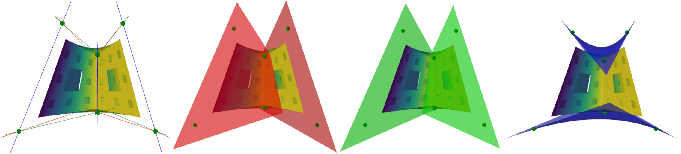
Figure 1: A deformation of a model, enclosed inside the unit cube, by means of a trilinear rational map. Leftmost: the boundary lines $s_{jk}$ (red), $t_{ik}$ (green), and $u_{ij}$ (blue), for each $0\leq i,j,k\leq 1$. From left to right: the boundary surfaces $\Sigma_{0},\Sigma_{1}$ (red), $T_{0},T_{1}$ (green), and $Y_{0},Y_{1}$ (blue).

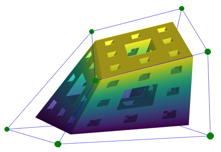
(a) A hexahedral rational map

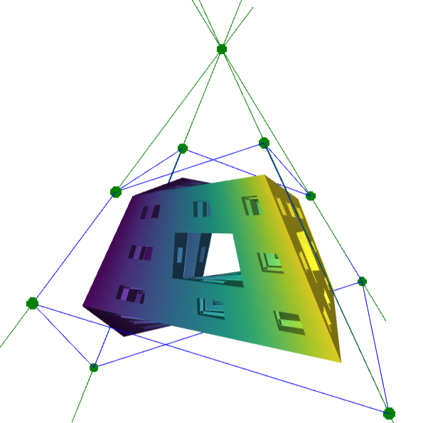
(b) A pyramidal rational map

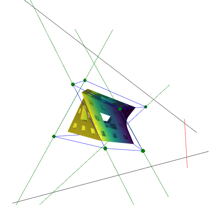
(c) A scaffold rational map

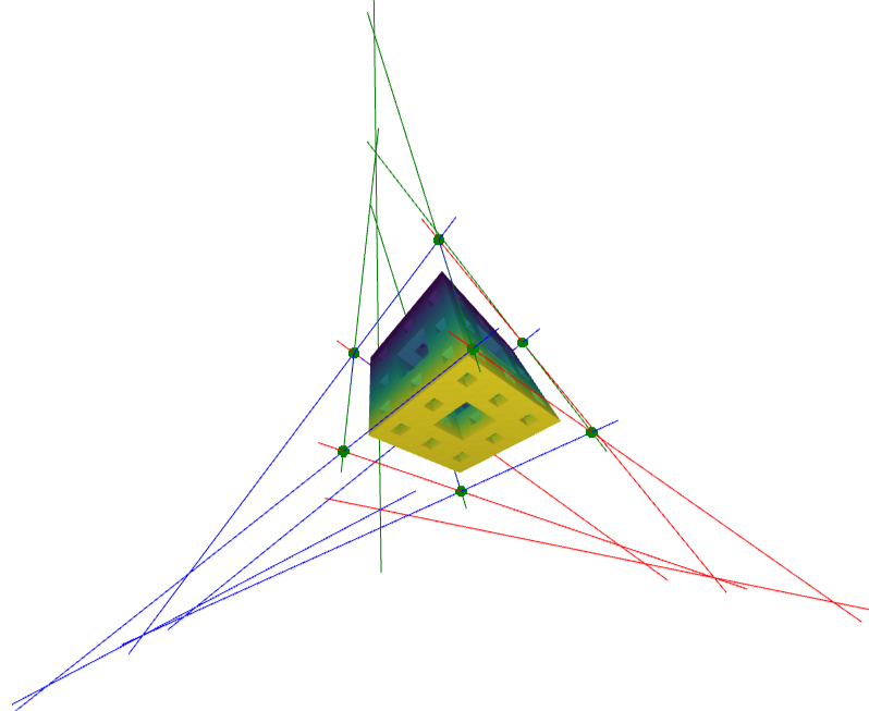
(d) A tripod rational map

Figure 2: The distinct geometric constraints on the control points that are necessary for birationality.

The geometry of rational maps can be rather complex, and in some degenerate cases the geometric intuition behind the boundary lines and surfaces can be lost. Specifically, it can occur that a boundary surface (resp. line) is not a surface (resp. line), but a curve (resp. point) due to a contraction. To avoid this scenario, we always require the following nondegeneracy property.

The following conditions are satisfied by a trilinear rational map:

1. For every $0\leq i,j,k\leq 1$, $\Sigma_{i}$, $T_{j}$, and $Y_{k}$ are smooth surfaces, pairwise distinct

2. For every $0\leq i,j,k\leq 1$, $s_{jk}$, $t_{ik}$, and $u_{ij}$ are lines, pairwise distinct

Notice that the previous property is not at all strict. Namely, it is satisfied by a general trilinear rational map. Furthermore, we can always ensure that it holds by composing with an automorphism of $(\mathbb{P}^{1})^{3}$.

In order to simplify the notation, we adopt the standard monomial basis in $R_{(1,1,1)}$, namely the $\mathbb{R}$-vector space of trilinear polynomials in $R$, instead of the Bernstein basis. These two formulations are equivalent after an obvious change of coordinates on each factor of $(\mathbb{P}^{1})^{3}$, and their analysis is hence identical. Nevertheless, the usage of the Bernstein basis is inherent to the geometric intuition behind the rational transformation of a cube, and thus to § 2.1. With this caveat in mind, for all the pictures and the examples of § 7 we recover the Bernstein basis.

We adopt the following conventions:

1. We always assume that $\phi:\mathbb{P}^{1}\times\mathbb{P}^{1}\times\mathbb{P}^{1}\dashrightarrow\mathbb{P}^{3}$ is the trilinear rational map defined by

   $$\mathbf{f}=(f_{0},f_{1},f_{2},f_{3})=\sum_{0\leq i,j,k\leq 1}w_{ijk}\,\mathbf{P}_{ijk}\,s_{i}t_{j}u_{k}$$

   for some $\mathbf{P}_{ijk}=(1,x_{ijk},y_{ijk},z_{ijk})$ in $\mathbb{R}^{4}$ and $w_{ijk}$ in $\mathbb{R}$, for each $0\leq i,j,k\leq 1$

2. $\Sigma_{i}$ (resp. $T_{j}$ and $Y_{k}$) is the closure of $\phi(\mathbb{P}^{1}\times\mathbb{P}^{1})$ for the specialization at $s_{i}=0$ (resp. $t_{j}=0$ and $u_{k}=0$)

3. $s_{jk}$ (resp. $t_{ik}$ and $u_{ij}$) is the closure of $\phi(\mathbb{P}^{1})$ for the specializations at $t_{j}=u_{k}=0$ (resp. $s_{i}=u_{k}=0$ and $s_{i}=t_{j}=0$)

4. If $\Sigma_{i}$ is a plane, it is defined by the linear form $\sigma_{i}=\boldsymbol{\sigma}_{i}\cdot\mathbf{x}^{T}$ for some $\boldsymbol{\sigma}_{i}=(\sigma_{0i},\sigma_{1i},\sigma_{2i},\sigma_{3i})$ in $\mathbb{R}^{4}$

5. If $\Sigma_{i}$ is a quadric, it is defined by the form $\sigma_{i}=\mathbf{x}\cdot\boldsymbol{\sigma}_{i}\cdot\mathbf{x}^{T}$ for some symmetric $4\times 4$ matrix in $\mathbb{R}^{4\times 4}$

6. Analogously, we denote by $\tau_{j},\upsilon_{k}$ the defining polynomials of $T_{j}$ and $Y_{k}$, and $\boldsymbol{\tau}_{j},\boldsymbol{\upsilon}_{k}$ their associated vectors and symmetric matrices

7. $\mathfrak{N}=(s_{0},s_{1})\cap(t_{0},t_{1})\cap(u_{0},u_{1})$ is the irrelevant ideal in $R$

2.2 Trilinear birational maps

If $\phi$ is birational, the inverse $\phi^{-1}$ has the form

(4) $$\phi^{-1}:\mathbb{P}^{3} \dashrightarrow \mathbb{P}^{1}\times\mathbb{P}^{1}\times\mathbb{P}^{1}$$

$$(x_{0}:x_{1}:x_{2}:x_{3}) \mapsto (A_{0}:A_{1})\times(B_{0}:B_{1})\times(C_{0}:C_{1})\ ,$$

where $A_{i}=A_{i}(\mathbf{x})$ (resp. $B_{j}=B_{j}(\mathbf{x})$ and $C_{k}=C_{k}(\mathbf{x})$) are homogeneous of the same degree for $i=0,1$ (resp. $j=0,1$ and $k=0,1$), without a common factor.

If $\phi$ is birational, the type of $\phi$ is the triple $(\deg A_{i},\deg B_{j},\deg C_{k})$ in $\mathbb{Z}^{3}$.

The defining polynomials of $\phi^{-1}$ are either linear or quadratic, and each type determines a class of trilinear birational maps [6]. Hence, there are only four possibilities up to permutation: $(1,1,1)$, $(1,1,2)$, $(1,2,2)$, and $(2,2,2)$. On the other hand, the composition $\phi^{-1}\circ\phi:(\mathbb{P}^{1})^{3}\dasharrow(\mathbb{P}^{1})^{3}$ yields the identity on some open set of $(\mathbb{P}^{1})^{3}$. Namely, $\phi^{-1}\circ\phi$ is generically given by

$$(s_{0}:s_{1})\times(t_{0}:t_{1})\times(u_{0}:u_{1}) \mapsto (A_{0}(\mathbf{f}):A_{1}(\mathbf{f}))\times(B_{0}(\mathbf{f}):B_{1}(\mathbf{f}))\times(C_{0}(\mathbf{f}):C_{1}(\mathbf{f}))$$

$$= (s_{0}:s_{1})\times(t_{0}:t_{1})\times(u_{0}:u_{1})\ .$$

Therefore, the $2\times 2$ determinants in $R[x_{0},x_{1},x_{2},x_{3}]=\mathbb{R}[s_{0},s_{1},t_{0},t_{1},u_{0},u_{1},x_{0},x_{1},x_{2},x_{3}]$

(5) $$\begin{vmatrix}s_{0}&s_{1}\\ A_{0}&A_{1}\end{vmatrix}\ \ ,\ \ \begin{vmatrix}t_{0}&t_{1}\\ B_{0}&B_{1}\end{vmatrix}\ \ ,\ \ \begin{vmatrix}u_{0}&u_{1}\\ C_{0}&C_{1}\end{vmatrix}$$

vanish with the specializations $x_{n}\mapsto f_{n}$ for each $0\leq n\leq 3$. In particular, they represent algebraic relations satisfied by the defining polynomials of $\phi$. More explicitly, if $\sigma_{0},\sigma_{1}$ (resp. $\tau_{0},\tau_{1}$ and $\upsilon_{0},\upsilon_{1}$) are linear, then the first (resp. second and third) relation is a syzygy of degree $(1,0,0)$ (resp. $(0,1,0)$ and $(0,0,1)$). Recall that a tuple $\boldsymbol{\pi}=(\pi_{0},\pi_{1},\pi_{2},\pi_{3})$ in $R^{4}$ of homogeneous polynomials of the same degree is a syzygy of $\mathbf{f}$ if

$$\langle\boldsymbol{\pi},\mathbf{f}\rangle=\boldsymbol{\pi}\cdot\mathbf{f}^{T}=\pi_{0}f_{0}+\pi_{1}f_{1}+\pi_{2}f_{2}+\pi_{3}f_{3}=0\ ,$$

where $\langle-,-\rangle$ stands for the usual scalar product. The $\mathbb{Z}^{3}$-degree of the polynomials in $\boldsymbol{\pi}$ is the degree of the syzygy. Equivalently, the syzygies of $\mathbf{f}$ are identified with the linear polynomials in $R[x_{0},x_{1},x_{2},x_{3}]$ that vanish after the specializations $x_{n}\mapsto f_{n}$ for each $0\leq n\leq 3$. Hence, the first (resp. second and third) determinant in Eq. 5 can be regarded as a syzygy.

If the defining polynomials of $\phi^{-1}$ are quadratic, the determinants in Eq. 5 correspond to more complicated relations in the defining ideal of the Rees algebra associated to $\phi$ (see [6]). Remarkably, the birationality of a trilinear rational map can be characterized using exclusively syzygies, without requiring quadratic relations. In our analysis, we take advantage of the following syzygy-based birationality criteria.

[6, Theorem 6.1] Let $\phi$ be dominant. Then, $\phi$ is birational if and only if one of the following conditions holds (up to permutation of the type of $\phi$):

1. $\mathbf{f}$ has syzygies of degrees $(1,0,0)$, $(0,1,0)$, and $(0,0,1)$. In this case, $\phi$ has type $(1,1,1)$.

2. $\mathbf{f}$ has syzygies of degrees $(1,0,0)$ and $(0,1,0)$, but not $(0,0,1)$. In this case, $\phi$ has type $(1,1,2)$.

3. $\mathbf{f}$ has a syzygy of degree $(1,0,0)$, but neither $(0,1,0)$ nor $(0,0,1)$. Moreover, $\mathbf{f}$ has a syzygy of degree either $(1,1,0)$ or $(1,0,1)$, independent from the first one. In this case, $\phi$ has type $(1,2,2)$.

4. $\mathbf{f}$ does not have linear syzygies. Moreover, $\mathbf{f}$ has two independent syzygies in each bilinear $\mathbb{Z}^{3}$-degree, satisfying an additional splitting condition. In this case, $\phi$ has type $(2,2,2)$.

Geometrically, the determinants in Eq. 5 define the implicit equations of the parametric surfaces. More explicitly, given a general $(s_{0}:s_{1})=(\lambda_{0}:\lambda_{1})$ in $\mathbb{P}^{1}$, the equation of the corresponding $s$-surface in $\mathbb{P}^{3}$ is

$$\begin{vmatrix}\lambda_{0}&\lambda_{1}\\ A_{0}&A_{1}\end{vmatrix}=0\ ,$$

and similarly for the $t$- and $u$-surfaces. In particular, the $s$-surfaces (resp. $t$- and $u$-surfaces) form the pencil, or linear system, of surfaces spanned by $\Sigma_{0},\Sigma_{1}$ (resp. $T_{0},T_{1}$ and $Y_{0},Y_{1}$).

Regarding the construction of birational maps, the challenge lies in reconciling the necessary algebraic relations involved in birationality with the representation of $\phi$ relying on control points and weights. As we shall prove, these relations impose geometric constraints on the control points, that are formalized in the following four classes of trilinear rational maps: hexahedral, pyramidal, scaffold, and tripod (see § 3, § 4, § 5, and § 6). Each of these classes are depicted in Figure 2, and respectively correspond to birational maps of type $(1,1,1)$, $(1,1,2)$, $(1,2,2)$, and $(2,2,2)$ (see § 4.1, § 5.1, and § 6.1). More precisely, by [6, Theorem 4.1] the locus of trilinear birational maps can be endowed with the structure of a locally closed algebraic subset of $\textnormal{Gr}(4,R_{(1,1,1)})\times\mathbb{P}^{15}$, and has eight irreducible components of dimensions 21 (for maps of type $(1,1,1)$), 22 (for types $(1,1,2)$, $(1,2,1)$, and $(2,1,1)$), and 23 (for types $(1,2,2)$, $(2,1,2)$, $(2,2,1)$, and $(2,2,2)$). In § 3 - § 6, we prove that the loci of hexahedral, pyramidal, scaffold, and tripod birational maps contain open subsets of these irreducible components. Our target is to construct all the birational transformations within each of these open sets.

Two central concepts in the study of birational maps are the base ideal and the base locus. In our context, these can be introduced as follows.

Maintaining the notation of the section:

1. The base ideal of $\phi$ is $I=(f_{0},f_{1},f_{2},f_{3})\subset R$

2. The base locus of $\phi$ is the subscheme of $(\mathbb{P}^{1})^{3}$ defined by $I$

3. The base ideal of $\phi^{-1}$ is $J=(A_{0},A_{1})\cap(B_{0},B_{1})\cap(C_{0},C_{1})\subset\mathbb{R}[x_{0},x_{1},x_{2},x_{3}]$

4. The base locus of $\phi^{-1}$ is the subscheme of $\mathbb{P}^{3}$ defined by $J$

The following classification result is used in the proofs of § 4.1, § 5.1, and § 6.1. In the statements of these results, when we refer to a “general birational map” of a fixed type, we precisely mean a birational lying in an open set where both § 2.1 and the following classification result hold (see [6] for a complete classification of the base loci of trilinear birational maps).

[6, Theorems $5.4$, $5.6$, and $5.8$] We assume $0\leq i,j,k\leq 1$.

1. The base locus of a general trilinear birational map of type $(1,1,1)$ is defined by the ideal

   $$(b_{0}s_{0}+b_{1}s_{1},c_{0}s_{0}+c_{1}s_{1},b_{0}c_{1}-b_{1}c_{0})$$

   for some linear $b_{j}=b_{j}(t_{0},t_{1})$ and $c_{k}=c_{k}(u_{0},u_{1})$

2. The base locus of a general trilinear birational map of type $(1,1,2)$ is defined by the ideal

   $$(a_{0},b_{0},c_{0})\cap(h,c_{1})$$

   for some linear $a_{0}=a_{0}(s_{0},s_{1})$, $b_{0}=b_{0}(t_{0},t_{1})$, $c_{k}=c_{k}(u_{0},u_{1})$, and bilinear irreducible $h=h(s_{0},s_{1},t_{0},t_{1})$

3. The base locus of a general trilinear birational map of type $(1,2,2)$ is defined by the ideal

   $$(a_{0},b_{0},c_{0})\cap(a_{1},b_{1},c_{1})\cap(b_{2},c_{2})$$

   for some linear $a_{i}=a_{i}(s_{0},s_{1})$, $b_{j}=b_{j}(t_{0},t_{1})$, and $c_{k}=c_{k}(u_{0},u_{1})$

4. The base locus of a general trilinear birational map of type $(2,2,2)$ is defined by the ideal

   $$(a_{0},b_{0},c_{0})\cap(a_{1}^{2},b_{1}^{2},c_{1}^{2},a_{1}b_{1},a_{1}c_{1},b_{1}c_{1},a_{1}b_{0}c_{0}+a_{0}b_{1}c_{0}+a_{0}b_{0}c_{1})$$

   for some linear $a_{i}=a_{i}(s_{0},s_{1})$, $b_{j}=b_{j}(t_{0},t_{1})$, and $c_{k}=c_{k}(u_{0},u_{1})$

2.3 Linear syzygies

By “linear syzygies” we mean syzygies of degrees $(1,0,0)$, $(0,1,0)$, and $(0,0,1)$. The following lemma characterizes the existence of a linear syzygy of $\mathbf{f}$ by means of a matrix rank condition. It is stated for syzygies of degree $(1,0,0)$, but it can be easily reformulated for syzygies of degrees $(0,1,0)$ and $(0,0,1)$ (see Remark 2.2).

Let $\phi$ be dominant and $\Sigma_{0},\Sigma_{1}$ be planes. Then, $\mathbf{f}$ has a syzygy of degree $(1,0,0)$ if and only if

(6) $$\mathrm{rank}\begin{pmatrix}w_{100}\,\langle\boldsymbol{\sigma}_{0},\mathbf{P}_{100}\rangle&w_{110}\,\langle\boldsymbol{\sigma}_{0},\mathbf{P}_{110}\rangle&w_{101}\,\langle\boldsymbol{\sigma}_{0},\mathbf{P}_{101}\rangle&w_{111}\,\langle\boldsymbol{\sigma}_{0},\mathbf{P}_{111}\rangle\\ w_{000}\,\langle\boldsymbol{\sigma}_{1},\mathbf{P}_{000}\rangle&w_{010}\,\langle\boldsymbol{\sigma}_{1},\mathbf{P}_{010}\rangle&w_{001}\,\langle\boldsymbol{\sigma}_{1},\mathbf{P}_{001}\rangle&w_{011}\,\langle\boldsymbol{\sigma}_{1},\mathbf{P}_{011}\rangle\end{pmatrix}=1\ .$$

Moreover, if (6) holds we find a point $(\alpha_{0}:\alpha_{1})$ in $\mathbb{P}{R}^{1}$ such that

(7) $$-\alpha_{0}\,w_{1jk}\,\langle\boldsymbol{\sigma}_{0},\mathbf{P}_{1jk}\rangle=\alpha_{1}\,w_{0jk}\,\langle\boldsymbol{\sigma}_{1},\mathbf{P}_{0jk}\rangle$$

for every $0\leq j,k\leq 1$. Then, any syzygy of degree $(1,0,0)$ of $\mathbf{f}$ is proportional to

(8) $$\boldsymbol{\sigma}=\boldsymbol{\sigma}(s_{0},s_{1})=\alpha_{0}\,\boldsymbol{\sigma}_{0}\,s_{0}+\alpha_{1}\,\boldsymbol{\sigma}_{1}\,s_{1}\ .$$

Proof 2.1.

For each $i=0,1$, we define

$$\mathbf{f}_{i}=\mathbf{f}_{i}(t_{0},t_{1},u_{0},u_{1})=\sum_{0\leq j,k\leq 1}w_{ijk}\,\mathbf{P}_{ijk}\,t_{j}u_{k}\ ,$$

so that we can easily write $\mathbf{f}=\mathbf{f}_{0}\,s_{0}+\mathbf{f}_{1}\,s_{1}$. Suppose that $\mathbf{f}$ has a syzygy of the form

$$\boldsymbol{\pi}=\boldsymbol{\pi}(s_{0},s_{1})=\boldsymbol{\pi}_{0}\,s_{0}+\boldsymbol{\pi}_{1}\,s_{1}$$

for some $\boldsymbol{\pi}_{0},\boldsymbol{\pi}_{1}$ in $\mathbb{R}^{4}$. Then, we find

$$\langle\boldsymbol{\pi},\mathbf{f}\rangle=s_{0}\,\langle\boldsymbol{\pi}_{0},\mathbf{f}\rangle+s_{1}\,\langle\boldsymbol{\pi}_{1},\mathbf{f}\rangle=s_{0}^{2}\,\langle\boldsymbol{\pi}_{0},\mathbf{f}_{0}\rangle+s_{0}s_{1}\,(\langle\boldsymbol{\pi}_{0},\mathbf{f}_{1}\rangle+\langle\boldsymbol{\pi}_{1},\mathbf{f}_{0}\rangle)+s_{1}^{2}\,\langle\boldsymbol{\pi}_{1},\mathbf{f}_{1}\rangle=0\ .$$

It follows immediately that $\langle\boldsymbol{\pi}_{i},\mathbf{f}_{i}\rangle=0$ for both $i=0,1$. By hypothesis, the boundary surfaces $\Sigma_{0},\Sigma_{1}$ are planes. Therefore, $\mathbf{f}_{i}$ defines a bilinear rational parametrization $\mathbb{P}^{1}\times\mathbb{P}^{1}\dashrightarrow\Sigma_{i}$, and any vector $\boldsymbol{\pi}$ satisfying $\langle\boldsymbol{\pi},\mathbf{f}_{i}\rangle=0$ must be proportional to $\boldsymbol{\sigma}_{i}$. In particular, we find $\boldsymbol{\pi}_{i}=\alpha_{i}\,\boldsymbol{\sigma}_{i}$ for some nonzero $\alpha_{i}$ in $\mathbb{R}$. Hence, we obtain

$$\alpha_{0}\langle\boldsymbol{\sigma}_{0},\mathbf{f}_{1}\rangle+\alpha_{1}\langle\boldsymbol{\sigma}_{1},\mathbf{f}_{0}\rangle=\sum_{0\leq j,k\leq 1}\left(\alpha_{0}\,w_{1jk}\,\langle\boldsymbol{\sigma}_{0},\mathbf{P}_{1jk}\rangle+\alpha_{1}\,w_{0jk}\,\langle\boldsymbol{\sigma}_{1},\mathbf{P}_{0jk}\rangle\right)t_{j}u_{k}=0\ ,$$

which is satisfied for some $\alpha_{0},\alpha_{1}$ if and only if Eq. 6 holds. Moreover, since $\phi$ is dominant no row in Eq. 6 is identically zero. Thus, $(\alpha_{0}:\alpha_{1})\in\mathbb{P}{R}^{1}$ is unique, and $\boldsymbol{\pi}$ is proportional to $\boldsymbol{\sigma}$.

Remark 2.2.

After the obvious modifications, we derive analogous results to § 2.3 for syzygies of degrees $(0,1,0)$ and $(0,0,1)$. The rank conditions involved in the existence of the syzygies are respectively

(9) $$\mathrm{rank}\begin{pmatrix}w_{010}\,\langle\boldsymbol{\tau}_{0},\mathbf{P}_{010}\rangle&w_{110}\,\langle\boldsymbol{\tau}_{0},\mathbf{P}_{110}\rangle&w_{011}\,\langle\boldsymbol{\tau}_{0},\mathbf{P}_{011}\rangle&w_{111}\,\langle\boldsymbol{\tau}_{0},\mathbf{P}_{111}\rangle\\ w_{000}\,\langle\boldsymbol{\tau}_{1},\mathbf{P}_{000}\rangle&w_{100}\,\langle\boldsymbol{\tau}_{1},\mathbf{P}_{100}\rangle&w_{001}\,\langle\boldsymbol{\tau}_{1},\mathbf{P}_{001}\rangle&w_{101}\,\langle\boldsymbol{\tau}_{1},\mathbf{P}_{101}\rangle\end{pmatrix}=1\ ,$$

(10) $$\mathrm{rank}\begin{pmatrix}w_{001}\,\langle\boldsymbol{\upsilon}_{0},\mathbf{P}_{001}\rangle&w_{101}\,\langle\boldsymbol{\upsilon}_{0},\mathbf{P}_{101}\rangle&w_{011}\,\langle\boldsymbol{\upsilon}_{0},\mathbf{P}_{011}\rangle&w_{111}\,\langle\boldsymbol{\upsilon}_{0},\mathbf{P}_{111}\rangle\\ w_{000}\,\langle\boldsymbol{\upsilon}_{1},\mathbf{P}_{000}\rangle&w_{100}\,\langle\boldsymbol{\upsilon}_{1},\mathbf{P}_{100}\rangle&w_{010}\,\langle\boldsymbol{\upsilon}_{1},\mathbf{P}_{010}\rangle&w_{110}\,\langle\boldsymbol{\upsilon}_{1},\mathbf{P}_{110}\rangle\end{pmatrix}=1\ .$$

3 Hexahedral birational maps

In this section, we study the first and simplest family of trilinear birational maps: the class of hexahedral birational maps, illustrated in Figure 2 top-left.

A trilinear rational map is hexahedral if it satisfies § 2.1 and all the boundary surfaces are planes.

Hexahedral birational maps are the direct generalization to 3D of the 2D quadrilateral birational maps studied in [44, 4], since the minimal graded free resolution of their base ideal is Hilbert-Burch [6, Proposition 6.2].

3.1 Geometric constraints

We begin describing the geometric constraints on the control points that are necessary for birationality. The following observation is straightforward.

Fact 1.

If $\phi$ is birational of type $(1,1,1)$, the parametric surfaces (and in particular the boundary surfaces) are planes (recall § 2.2). If it additionally satisfies § 2.1, then it is hexahedral.

In practice, the control points of a hexahedral map can be given indirectly through the boundary planes $\Sigma_{i}$, $T_{j}$, $Y_{k}$. More explicitly, we have the following construction.

The control points of a hexahedral rational map can be generated as follows:

1. For each $0\leq i,j,k\leq 1$, choose pairwise distinct planes $\Sigma_{i}$, $T_{j}$, $Y_{k}$ whose intersection is an affine point

2. Define $\mathbf{P}_{ijk}=\Sigma_{i}\cap T_{j}\cap Y_{k}$

3.2 Birational weights and tensor rank criterion

If $\phi$ is hexahedral, $\mathbf{P}_{ijk}$ can be expressed as the wedge of the vectors $\boldsymbol{\sigma}_{i}$, $\boldsymbol{\tau}_{j}$, and $\boldsymbol{\upsilon}_{k}$ defining the boundary planes. More specifically, we have

(11) $$\mathbf{P}_{ijk}=\Delta_{ijk}^{-1}\ \boldsymbol{\sigma}_{i}\wedge\boldsymbol{\tau}_{j}\wedge\boldsymbol{\upsilon}_{k}\ ,$$

where

(12) $$\Delta_{ijk}=\begin{vmatrix}\sigma_{1i}&\sigma_{2i}&\sigma_{3i}\\ \tau_{1j}&\tau_{2j}&\tau_{3j}\\ \upsilon_{1k}&\upsilon_{2k}&\upsilon_{3k}\end{vmatrix}$$

for each $0\leq i,j,k\leq 1$. In particular, $\Delta_{ijk}=0$ if and only if $\mathbf{P}_{ijk}$ lies at the plane $x_{0}=0$ in $\mathbb{P}^{3}$, a possibility is excluded since by definition $\mathbf{P}_{ijk}=(1,x_{ijk},y_{ijk},z_{ijk})$.

The following theorem establishes our birationality criterion for the class of hexahedral rational maps, based on a rank-one condition on a $2\times 2\times 2$ tensor. It relates birationality, the existence of linear syzygies, and tensor rank. Moreover, it is the key ingredient for our constructive results. We refer the reader to [33, 27, 38, 39, 39, 32] for a global perspective about tensor rank.

Let $\phi$ be hexahedral. Then, $\phi$ is birational of type $(1,1,1)$ if and only if the $2\times 2\times 2$ tensor

(13) $$W=\left(\frac{w_{ijk}}{\Delta_{ijk}}\right)_{0\leq i,j,k\leq 1}$$

has rank one.

Proof 3.1.

By § 2.2, $\phi$ is birational of type $(1,1,1)$ if and only if $\mathbf{f}$ admits syzygies of degrees $(1,0,0)$, $(0,1,0)$, and $(0,0,1)$. Equivalently, by § 2.3 and Remark 2.2, $\phi$ is birational if and only if the matrix rank conditions Eq. 6, Eq. 9, and Eq. 10 are simultaneously satisfied. We now rewrite these rank conditions so that the matrices involved have the same entries. Namely, for any $0\leq i,j,k\leq 1$ we can write

(14) $$\Delta_{0jk}\,\langle\boldsymbol{\sigma}_{1},\mathbf{P}_{0jk}\rangle=\boldsymbol{\sigma}_{1}\wedge\boldsymbol{\sigma}_{0}\wedge\boldsymbol{\tau}_{j}\wedge\boldsymbol{\upsilon}_{k}=-\Delta_{1jk}\,\Delta_{1jk}^{-1}\,\boldsymbol{\sigma}_{0}\wedge\boldsymbol{\sigma}_{1}\wedge\boldsymbol{\tau}_{j}\wedge\boldsymbol{\upsilon}_{k}=-\Delta_{1jk}\,\langle\boldsymbol{\sigma}_{0},\mathbf{P}_{1jk}\rangle\ .$$

Hence, we have

$$\begin{vmatrix}\langle\boldsymbol{\sigma}_{0},\mathbf{P}_{1jk}\rangle&-\langle\boldsymbol{\sigma}_{1},\mathbf{P}_{0jk}\rangle\\ \Delta_{0jk}&\Delta_{1jk}\end{vmatrix}=0\ ,$$

and Eq. 6 can be equivalently written as

(15) $$\mathrm{rank}\begin{pmatrix}w_{100}\,{\Delta_{100}}^{-1}&w_{110}\,{\Delta_{110}}^{-1}&w_{101}\,{\Delta_{101}}^{-1}&w_{111}\,{\Delta_{111}}^{-1}\\ w_{000}\,{\Delta_{000}}^{-1}&w_{010}\,{\Delta_{010}}^{-1}&w_{001}\,{\Delta_{001}}^{-1}&w_{011}\,{\Delta_{011}}^{-1}\end{pmatrix}=1\ .$$

With a similar argument, we derive

$$\Delta_{i0k}\,\langle\boldsymbol{\tau}_{1},\mathbf{P}_{i0k}\rangle=-\Delta_{i1k}\,\langle\boldsymbol{\tau}_{0},\mathbf{P}_{i1k}\rangle\ \ ,\ \ \Delta_{ij0}\,\langle\boldsymbol{\upsilon}_{1},\mathbf{P}_{ij0}\rangle=-\Delta_{ij1}\,\langle\boldsymbol{\upsilon}_{0},\mathbf{P}_{ij1}\rangle\ ,$$

and Eq. 9, Eq. 10 can be respectively rewritten as

(16) $$\mathrm{rank}\begin{pmatrix}w_{010}\,{\Delta_{010}}^{-1}&w_{110}\,{\Delta_{110}}^{-1}&w_{011}\,{\Delta_{011}}^{-1}&w_{111}\,{\Delta_{111}}^{-1}\\ w_{000}\,{\Delta_{000}}^{-1}&w_{100}\,{\Delta_{100}}^{-1}&w_{001}\,{\Delta_{001}}^{-1}&w_{101}\,{\Delta_{101}}^{-1}\end{pmatrix}=1\ ,$$

(17) $$\mathrm{rank}\begin{pmatrix}w_{001}\,{\Delta_{001}}^{-1}&w_{101}\,{\Delta_{101}}^{-1}&w_{011}\,{\Delta_{011}}^{-1}&w_{111}\,{\Delta_{111}}^{-1}\\ w_{000}\,{\Delta_{000}}^{-1}&w_{100}\,{\Delta_{100}}^{-1}&w_{010}\,{\Delta_{010}}^{-1}&w_{110}\,{\Delta_{110}}^{-1}\end{pmatrix}=1\ .$$

In particular, the matrices involved in the three rank conditions above are the three flattenings of the tensor $W$ in the statement (see [33, 39, 32]). By [39, Proposition $3.11$], they have all rank one if and only if $W$ has rank one, and the statement follows.

Let $\phi$ be hexahedral. Then, $\phi$ is birational of type $(1,1,1)$ if and only if

(18) $$w_{ijk}=\alpha_{i}\,\beta_{j}\,\gamma_{k}\,\Delta_{ijk}$$

for some $(\alpha_{0}:\alpha_{1})\times(\beta_{0}:\beta_{1})\times(\gamma_{0}:\gamma_{1})$ in $(\mathbb{P}{R}^{1})^{3}$.

3.3 Inverse and base locus

We now address the most relevant computational advantage of birational maps: the efficient and exact computation of preimages. The following result presents explicit formulas for the inverse of a hexahedral birational map. Moreover, it provides a minimal set of generators for the base ideal, and describes the contractions and blow-ups of the birational map. Specifically, we say that $\phi$ contracts, or blows down, a variety $V\subset(\mathbb{P}^{1})^{3}$ if $\dim V>\dim\phi(V)$.

Let $\phi$ be hexahedral with weights as Eq. 18. Then, $\phi^{-1}$ is given by

(19) $$(x_{0}:x_{1}:x_{2}:x_{3})\mapsto(-\alpha_{1}\,\sigma_{1}:\alpha_{0}\,\sigma_{0})\times(-\beta_{1}\,\tau_{1}:\beta_{0}\,\tau_{0})\times(-\gamma_{1}\,\upsilon_{1}:\gamma_{0}\,\upsilon_{0})\ .$$

Additionally, we have the following:

1. The base locus of $\phi$ is the curve $C$ in $(\mathbb{P}^{1})^{3}$ defined by the ideal

   (20) $$I:\mathfrak{N}^{\infty}=\left(\sum_{0\leq j,k\leq 1}w_{0jk}\langle\boldsymbol{\sigma}_{1},\mathbf{P}_{0jk}\rangle\,t_{j}u_{k}\,,\,\sum_{0\leq i,k\leq 1}w_{i0k}\langle\boldsymbol{\tau}_{1},\mathbf{P}_{i0k}\rangle\,s_{i}u_{k}\,,\,\sum_{0\leq i,j\leq 1}w_{ij0}\langle\boldsymbol{\upsilon}_{1},\mathbf{P}_{ij0}\rangle\,s_{i}t_{j}\right)$$

2. The base locus of $\phi^{-1}$ is the union of the lines $s=\Sigma_{0}\cap\Sigma_{1}$, $t=T_{0}\cap T_{1}$, and $u=Y_{0}\cap Y_{1}$

3. $\phi$ contracts the surfaces in $(\mathbb{P}^{1})^{3}$ defined by the first, second, and third generators of the right-hand side of Eq. 20 respectively to the lines $s,t$, and $u$

4. If $s,t$, and $u$ are pairwise skew, then $\phi$ blows up $C$ to the unique (smooth) quadric through them

Proof 3.2.

By § 3.2, a hexahedral rational map is birational if and only if the weights satisfy Eq. 18 for some $(\alpha_{0}:\alpha_{1})\times(\beta_{0}:\beta_{1})\times(\gamma_{0}:\gamma_{1})$ in $(\mathbb{P}{R}^{1})^{3}$. In particular, we can write

$$\mathbf{f}=\sum_{0\leq i,j,k\leq 1}w_{ijk}\,\mathbf{P}_{ijk}\,s_{i}t_{j}u_{k}=\sum_{0\leq i,j,k\leq 1}\left(\alpha_{i}\,\beta_{j}\,\gamma_{k}\,\Delta_{ijk}\right)\,\left(\Delta_{ijk}^{-1}\,\boldsymbol{\sigma}_{i}\wedge\boldsymbol{\tau}_{j}\wedge\boldsymbol{\upsilon}_{k}\right)\,s_{i}t_{j}u_{k}=$$

$$\sum_{0\leq i,j,k\leq 1}(\alpha_{i}\,\boldsymbol{\sigma}_{i}\,s_{i})\wedge(\beta_{i}\,\boldsymbol{\tau}_{j}\,t_{j})\wedge(\gamma_{k}\,\boldsymbol{\upsilon}_{k}\,u_{k})=\boldsymbol{\sigma}(s_{0},s_{1})\wedge\boldsymbol{\tau}(t_{0},t_{1})\wedge\boldsymbol{\upsilon}(u_{0},u_{1})\ ,$$

where $\boldsymbol{\sigma}=\boldsymbol{\sigma}(s_{0},s_{1})$ is as in § 2.3 and $\boldsymbol{\tau}=\boldsymbol{\tau}(t_{0},t_{1})$, $\boldsymbol{\upsilon}=\boldsymbol{\upsilon}(u_{0},u_{1})$ are analogous. Therefore, we find

$$\langle\boldsymbol{\sigma},\mathbf{f}\rangle=\boldsymbol{\sigma}\wedge\boldsymbol{\sigma}\wedge\boldsymbol{\tau}\wedge\boldsymbol{\upsilon}=0\ \ ,\ \ \langle\boldsymbol{\tau},\mathbf{f}\rangle=\boldsymbol{\tau}\wedge\boldsymbol{\sigma}\wedge\boldsymbol{\tau}\wedge\boldsymbol{\upsilon}=0\ \ ,\ \ \langle\boldsymbol{\upsilon},\mathbf{f}\rangle=\boldsymbol{\upsilon}\wedge\boldsymbol{\sigma}\wedge\boldsymbol{\tau}\wedge\boldsymbol{\upsilon}=0\ \ ,$$

or equivalently, the polynomials in $R[x_{0},x_{1},x_{2},x_{3}]$

$$\alpha_{0}\,\sigma_{0}\,s_{0}+\alpha_{1}\,\sigma_{1}\,s_{1}=\begin{vmatrix}s_{0}&s_{1}\\ -\alpha_{1}\,\sigma_{1}&\alpha_{0}\,\sigma_{0}\end{vmatrix}\ \ ,\ \ \begin{vmatrix}t_{0}&t_{1}\\ -\beta_{1}\,\tau_{1}&\beta_{0}\,\tau_{0}\end{vmatrix}\ \ ,\ \ \begin{vmatrix}u_{0}&u_{1}\\ -\gamma_{1}\,\upsilon_{1}&\gamma_{0}\,\upsilon_{0}\end{vmatrix}$$

vanish after the specializations $x_{n}\mapsto f_{n}$ for every $0\leq n\leq 3$. Therefore, $\phi^{-1}$ is given by Eq. 19.

Now, we prove the remaining four claims. Let $i^{*}$ stand for the converse of a binary index, namely $0^{*}=1$ and $1^{*}=0$. Additionally, let $I^{\prime}$ be the ideal on the right-hand side of Eq. 20. For each $i=0,1$, we can write

(21) $$\langle\boldsymbol{\sigma}_{i},\mathbf{f}\rangle=s_{i^{*}}\sum_{0\leq j,k\leq 1}w_{i^{*}jk}\,\langle\boldsymbol{\sigma}_{i},\mathbf{P}_{i^{*}jk}\rangle\,t_{j}\,u_{k}=s_{i^{*}}\,g_{i}(t_{0},t_{1},u_{0},u_{1})$$

since by definition $\langle\boldsymbol{\sigma}_{i},\mathbf{P}_{ijk}\rangle=0$ for each $0\leq j,k\leq 1$. The coefficients of $g_{i}$ (in the monomial basis) coincide with the entries of the $(i+1)$-th row of the matrix in Eq. 6. Since $\mathbf{f}$ admits a syzygy of degree $(1,0,0)$, by § 2.3 the rank condition Eq. 6 holds. In particular, $g_{0}$ and $g_{1}$ are proportional to the first generator $g$ of $I^{\prime}$. Hence, we find

$$(\sigma_{0}(f_{0},f_{1},f_{2},f_{3})\,,\,\sigma_{1}(f_{0},f_{1},f_{2},f_{3})):\mathfrak{N}^{\infty}=(g)\ .$$

Geometrically, this means that $\phi$ contracts the surface in $(\mathbb{P}^{1})^{3}$ defined by $g=0$ to the line $s=\Sigma_{0}\cap\Sigma_{1}$, defined by the ideal $(\sigma_{0},\sigma_{1})\subset\mathbb{R}[x_{0},x_{1},x_{2},x_{3}]$. With parallel arguments, it follows that $\phi$ contracts the surfaces defined by the second and third generators of $I^{\prime}$ to the lines $t$ and $u$, respectively. By Eq. 21 and the analogous identities for the other two pairs of variables, we conclude that $I:\mathfrak{N}^{\infty}=I^{\prime}$. On the other hand, by definition the base ideal (resp. locus) of $\phi^{-1}$ is $(\sigma_{0},\sigma_{1})\cap(\tau_{0},\tau_{1})\cap(\upsilon_{0},\upsilon_{1})\subset\mathbb{R}[x_{0},x_{1},x_{2},x_{3}]$ (resp. $s\cup t\cup u$ in $\mathbb{P}^{3}$). Finally, since the composition $\phi\circ\phi^{-1}:\mathbb{P}^{3}\dashrightarrow\mathbb{P}^{3}$ yields the identity in an open set, the specializations

$$s_{i}\mapsto(-1)^{i^{*}}\alpha_{i^{*}}\,\sigma_{i^{*}}\ \ ,\ \ t_{j}\mapsto(-1)^{j^{*}}\beta_{j^{*}}\,\tau_{j^{*}}\ \ ,\ \ u_{k}\mapsto(-1)^{k^{*}}\gamma_{k^{*}}\,\upsilon_{k^{*}}$$

on $\mathbf{f}=(f_{0},f_{1},f_{2},f_{3})$ yield the vector of polynomials

$$(q\,x_{0}\,,\,q\,x_{1}\,,\,q\,x_{2}\,,\,q\,x_{3})$$

for some quadratic form $q=q(x_{0},x_{1},x_{2},x_{3})$ that vanishes at the three lines $s,t$, and $u$. If these are pairwise skew, then $q$ defines the unique quadric through the lines (see either [7, Corollary 8.3.19] or [28, Exercise 2.12]).

4 Pyramidal birational maps

We now study the second family of birational maps: the class of pyramidal birational maps, illustrated in Figure 2 top-right. This name is motivated by the geometry of the control points.

A trilinear rational map is pyramidal if it satisfies § 2.1 and for one of the three parameters:

1. The four boundary lines intersect at a point

2. The two boundary surfaces are quadrics

4.1 Geometric constraint

First, we prove that a general birational map of type either $(1,1,2)$, $(1,2,1)$, or $(2,1,1)$ is pyramidal. Without loss of generality, we can restrict to the first type.

If $\phi$ is a general birational map of type $(1,1,2)$, then it is pyramidal. Moreover,

$$Y_{0}\cap Y_{1}=s\cup t\cup C\ ,$$

where $s=\Sigma_{0}\cap\Sigma_{1}$, $t=T_{0}\cap T_{1}$, and $C$ is a plane conic that intersects both $s$ and $t$.

Proof 4.1.

Since $\phi$ is general, § 2.1 is satisfied. On the other hand, by § 2.2 we find

(22) $$I:\mathfrak{N}^{\infty}=(f_{0},f_{1},f_{2},f_{3}):\mathfrak{N}^{\infty}=(a_{0},b_{0},c_{0})\cap(h,c_{1})$$

for some linear $a_{0}=a_{0}(s_{0},s_{1})$, $b_{0}=b_{0}(t_{0},t_{1})$, $c_{k}=c_{k}(u_{0},u_{1})$ for $k=0,1$, and bilinear irreducible $h=h(s_{0},s_{1},t_{0},t_{1})$. Let $\phi^{-1}$ be defined by

$$(x_{0},x_{1},x_{2},x_{3})\mapsto(A_{0}:A_{1})\times(B_{0}:B_{1})\times(C_{0}:C_{1})$$

for some linear $A_{i}=A_{i}(\mathbf{x})$, $B_{j}=B_{j}(\mathbf{x})$ and quadratic $C_{k}=C_{k}(\mathbf{x})$. Since $\phi\circ\phi^{-1}:\mathbb{P}^{3}\dashrightarrow\mathbb{P}^{3}$ yields the identity in an open set, we find

$$(f_{0}(A_{0},A_{1},B_{0},B_{1},C_{0},C_{1})\,,\,\ldots\,,\,f_{3}(A_{0},A_{1},B_{0},B_{1},C_{0},C_{1}))=(F\,x_{0},F\,x_{1},F\,x_{2},F\,x_{3})$$

for some cubic form $F=F(\mathbf{x})$. Therefore, the pullback ideals

$$(a_{0}(A_{0},A_{1}),b_{0}(B_{0},B_{1}),c_{0}(C_{0},C_{1}))\ \ ,\ \ (h(A_{0},A_{1},B_{0},B_{1}),c_{1}(C_{0},C_{1}))$$

are principal in $\mathbb{R}[x_{0},x_{1},x_{2},x_{3}]$, and respectively generated by a linear and a quadratic form. In particular, the linear polynomials $a_{0}(A_{0},A_{1})$ and $b_{0}(B_{0},B_{1})$ are proportional, and define a plane $\Pi_{0}$. Geometrically, this means that the boundary planes $\Sigma_{0},\Sigma_{1},T_{0}$, and $T_{1}$ are not independent, and they intersect at a point $\mathbf{A}$ in $\mathbb{P}{R}^{3}$. Hence, the four boundary $u$-lines, $u_{ij}=\Sigma_{i}\cap T_{j}$ for each $0\leq i,j\leq 1$, intersect at $\mathbf{A}$, and $\phi$ is pyramidal.

Additionally, the quadratic polynomial $c_{0}(C_{0},C_{1})$ is divisible by $a_{0}(A_{0},A_{1})$ and $b_{0}(B_{0},B_{1})$. Therefore, $c_{0}(C_{0},C_{1})$ determines a rank-two quadric $\Pi_{0}\cup\Pi_{1}$ in the pencil of $u$-surfaces. On the other hand, the polynomials $c_{1}(C_{0},C_{1})$ and $h(A_{0},A_{1},B_{0},B_{1})$ are also proportional, and define a quadric $Q$. In particular, $Q$ contains the lines $s,t\subset\Pi_{0}$ since $h(A_{0},A_{1},B_{0},B_{1})$ vanishes at both. Hence, they lie in $Y_{0}\cap Y_{1}$. Furthermore, we have

$$Y_{0}\cap Y_{1}=(\Pi_{0}\cup\Pi_{1})\cap Q=(\Pi_{0}\cap Q)\cup(\Pi_{1}\cap Q)=s\cup t\cup C\ ,$$

where $\Pi_{1}\cap Q=C$ is a plane conic that intersects both $s$ and $t$.

In applications, the control points of a pyramidal map can be generated using the following construction.

The control points of a pyramidal rational map can be generated as follows:

1. Choose a point $\mathbf{A}$ in $\mathbb{P}{R}^{3}$

2. For each $0\leq i,j\leq 1$, choose pairwise distinct lines $u_{ij}$ in $\mathbb{P}{R}^{3}$ through $\mathbf{A}$ and not contained in $x_{0}=0$

3. For each $0\leq i,j\leq 1$, choose two distinct affine points $\mathbf{P}_{ij0}$ and $\mathbf{P}_{ij1}$ on $u_{ij}$, both different from $\mathbf{A}$

4.2 Birational weights and tensor rank criterion

In all the upcoming statements of this § 4, when $\phi$ is pyramidal we assume that $Y_{0},Y_{1}$ are the quadric boundary surfaces.

Let $\phi$ be pyramidal. We denote by $\Pi_{0}$ the plane through the lines $s=\Sigma_{0}\cap\Sigma_{1}$ and $t=T_{0}\cap T_{1}$, which is defined by $\pi_{0}=\boldsymbol{\pi}_{0}\cdot\mathbf{x}^{T}$ for some $\boldsymbol{\pi}_{0}$ in $\mathbb{R}^{4}$. In particular, we find points $(\lambda_{0}:\lambda_{1})$ and $(\mu_{0}:\mu_{1})$ in $\mathbb{P}{R}^{1}$ such that

$$\pi_{0}=\lambda_{0}\,\sigma_{0}+\lambda_{1}\,\sigma_{1}=\mu_{0}\,\tau_{0}+\mu_{1}\,\tau_{1}\ .$$

Additionally, for each $0\leq i,j,k\leq 1$ we set

$$\Delta_{ijk}=\frac{1}{\langle\boldsymbol{\pi}_{0},\mathbf{P}_{ijk}\rangle}\ .$$

Remark 4.2.

For pyramidal maps, $\Delta_{ijk}$ is well-defined for every $0\leq i,j,k\leq 1$. Specifically, $\Delta_{ijk}$ is not well-defined if and only if $\mathbf{P}_{ijk}=\mathbf{A}$, a possibility that is excluded by § 2.1. More explicitly, if $\mathbf{P}_{ijk}=\mathbf{A}$ then we find $s_{jk}=\overline{\mathbf{P}_{0jk}\mathbf{P}_{1jk}}=\overline{\mathbf{A}\mathbf{P}_{i^{*}jk}}=u_{i^{*}j}$, as well as $t_{ik}=u_{ij^{*}}$.

The following is the analogous birationality criterion to § 3.2 for the class of pyramidal rational maps.

Let $\phi$ be pyramidal. Then, $\phi$ is birational of type $(1,1,2)$ if and only if the $2\times 2\times 2$ tensor

$$W=\left(\frac{w_{ijk}}{\Delta_{ijk}}\right)_{0\leq i,j,k\leq 1}$$

has rank one.

Proof 4.3.

By § 2.2, $\phi$ is birational of type $(1,1,2)$ if and only if $\mathbf{f}$ admits syzygies of degrees $(1,0,0)$, $(0,1,0)$, but not $(0,0,1)$. Since $Y_{0}$ and $Y_{1}$ are smooth quadrics, $\mathbf{f}$ cannot have a syzygy of degree $(0,0,1)$. Therefore, by § 2.3 and Remark 2.2 $\phi$ is birational if and only if the matrix rank conditions Eq. 6 and Eq. 9 hold simultaneously. Once more, we rewrite these rank conditions in terms of the flattenings of $W$.

Recall that we let $0^{*}=1$ and $1^{*}=0$. For each $0\leq i,j,k\leq 1$, we can write

$$\lambda_{i^{*}}\langle\boldsymbol{\sigma}_{i^{*}},\mathbf{P}_{ijk}\rangle=\langle\lambda_{0}\,\boldsymbol{\sigma}_{0}+\lambda_{1}\,\boldsymbol{\sigma}_{1},\mathbf{P}_{ijk}\rangle=\langle\boldsymbol{\pi}_{0},\mathbf{P}_{ijk}\rangle=\Delta_{ijk}^{-1}\ ,$$

$$\mu_{j^{*}}\langle\boldsymbol{\tau}_{j^{*}},\mathbf{P}_{ijk}\rangle=\langle\mu_{0}\,\boldsymbol{\tau}_{0}+\mu_{1}\,\boldsymbol{\tau}_{1},\mathbf{P}_{ijk}\rangle=\langle\boldsymbol{\pi}_{0},\mathbf{P}_{ijk}\rangle=\Delta_{ijk}^{-1}\ .$$

Therefore, Eq. 6 and Eq. 9 are respectively equivalent to

$$\mathrm{rank}\begin{pmatrix}w_{1jk}\,\Delta_{1jk}^{-1}\\ w_{0jk}\,\Delta_{0jk}^{-1}\end{pmatrix}_{0\leq j,k\leq 1}=1\ \ ,\ \ \mathrm{rank}\begin{pmatrix}w_{i1k}\,\Delta_{i1k}^{-1}\\ w_{i0k}\,\Delta_{i0k}^{-1}\end{pmatrix}_{0\leq i,k\leq 1}=1\ ,$$

which are rank-one conditions on the first two flattenings of $W$. By [39, Proposition $3.11$], $W$ has rank one if and only if these two conditions are satisfied, and the result follows.

Let $\phi$ be pyramidal. Then, $\phi$ is birational of type $(1,1,2)$ if and only if

(23) $$w_{ijk}=\alpha_{i}\,\beta_{j}\,\gamma_{k}\,\Delta_{ijk}$$

for some $(\alpha_{0}:\alpha_{1})\times(\beta_{0}:\beta_{1})\times(\gamma_{0}:\gamma_{1})$ in $(\mathbb{P}{R}^{1})^{3}$.

4.2.1 The contractions of a pyramidal birational map

Let $\phi$ be pyramidal with weights as Eq. 23. By § 4.2, $\phi$ is birational of type $(1,1,2)$, and by § 4.1 the pencil of $u$-surfaces contains the following quadrics:

1. The rank-two quadric $\Pi_{0}\cup\Pi_{1}$, where $\Pi_{1}$ is the plane supporting the conic $C$. In particular, $\Pi_{1}$ is defined by $\pi_{1}=\boldsymbol{\pi}_{1}\cdot\mathbf{x}^{T}$ for some $\boldsymbol{\pi}_{1}$ in $\mathbb{R}^{4}$

2. The cone (rank-three quadric) $Q$ with apex $\mathbf{A}=s\cap t$ through the conic $C$. In particular, we find a $(\nu_{0}:\nu_{1})$ in $\mathbb{P}{R}^{1}$ such that $Q$ is defined by

   $$\nu_{0}\,\upsilon_{0}+\nu_{1}\,\upsilon_{1}$$

The rank-one condition of § 4.2 has a clear geometric interpretation, since it readily determines all the contractions of $\phi$.

Let $\phi$ be pyramidal with weights as Eq. 23. Then, we have

(24) $$\langle\boldsymbol{\pi}_{1},\mathbf{f}\rangle=h(s_{0},s_{1},t_{0},t_{1})\,c_{0}(u_{0},u_{1})$$

for some linear $c_{0}=c_{0}(u_{0},u_{1})$ and bilinear irreducible $h=h(s_{0},s_{1},t_{0},t_{1})$. Additionally, let

(25) $$a_{0}(s_{0},s_{1})=\begin{vmatrix}\phantom{-}s_{0}&s_{1}\\ -\alpha_{1}&\alpha_{0}\end{vmatrix}\ \ ,\ \ b_{0}(t_{0},t_{1})=\begin{vmatrix}\phantom{-}t_{0}&t_{1}\\ -\beta_{1}&\beta_{0}\end{vmatrix}\ \ ,\ \ c_{1}(u_{0},u_{1})=\begin{vmatrix}\phantom{-}u_{0}&u_{1}\\ -\gamma_{1}&\gamma_{0}\end{vmatrix}\ .$$

Then, we have the following:

1. $\phi$ contracts the surface $a_{0}=0$ to the line $t$

2. $\phi$ contracts the surface $b_{0}=0$ to the line $s$

3. $\phi$ contracts the surface $c_{1}=0$ to the point $\mathbf{A}=s\cap t$

4. $\phi$ contracts the surface $h=0$ to the plane conic $C$

5. The image of the surface $c_{0}=0$ is dense in $\Pi_{1}$

Proof 4.4.

By Eq. 23, we find

$$\langle\boldsymbol{\pi}_{0},\mathbf{f}\rangle=\sum_{0\leq i,j,k\leq 1}w_{ijk}\langle\boldsymbol{\pi}_{0},\mathbf{P}_{ijk}\rangle s_{i}t_{j}u_{k}=\sum_{0\leq i,j,k\leq 1}\left(\frac{w_{ijk}}{\Delta_{ijk}}\right)s_{i}t_{j}u_{k}=\sum_{0\leq i,j,k\leq 1}(\alpha_{i}s_{i})(\beta_{j}t_{j})(\gamma_{k}u_{k})=a_{0}b_{0}c_{1}\ .$$

By definition we have $\Sigma_{i}\cap\Pi_{0}=\Sigma_{0}\cap\Sigma_{1}=s$, and the boundary $t$-lines $t_{i0},t_{i1}$ lie in $\Sigma_{i}$ for each $i=0,1$. Hence, the four boundary $t$-lines intersect $\Pi_{0}$ at $s$. Therefore, as the image by $\phi$ of the surface $b_{0}=0$ lies in $\Pi_{0}$, it follows that $\phi$ contracts it to $s$. Similarly, it follows that $\phi$ contracts the surface $a_{0}=0$ to $t$. Additionally, the image of $c_{1}=0$ also lies in $\Pi_{0}$. Since the four boundary $u$-lines meet $\Pi_{0}$ at $\mathbf{A}$, we conclude that $\phi$ contracts $c_{1}=0$ to $\mathbf{A}$.

On the other hand, as $C$ lies in the base locus of $\phi^{-1}$ it follows that $\phi$ contracts some surface in $(\mathbb{P}^{1})^{3}$ to $C$. Let $h=0$ be this surface, for some multihomogeneous $h$ in $R$. Then, the ideal $(c_{1},h)\subset R$ defines a component of the base locus of $\phi$, since $C$ and $\mathbf{A}$ are disjoint. By § 2.2, it follows that $h=h(s_{0},s_{1},t_{0},t_{1})$ is bilinear and irreducible. In particular, the pullback of the plane $\Pi_{1}$ admits the factorization Eq. 24 for some linear $c_{0}=c_{0}(u_{0},u_{1})$. Furthermore, since $\phi$ is dominant the intersection points of the boundary $u$-lines with $\Pi_{1}$ are not colinear, and the image of $c_{0}=0$ is dense in $\Pi_{1}$.

4.3 Inverse and base locus

In this subsection, we derive formulas for the inverse of a pyramidal birational map, as well as the defining equations of the irreducible components of the base locus and the blow-ups.

Let $\phi$ be pyramidal with weights as Eq. 23. Then, $\phi^{-1}$ is given by

$$(x_{0}:x_{1}:x_{2}:x_{3})\mapsto\left(\alpha_{1}\,\lambda_{1}\,\sigma_{1}:\alpha_{0}\,\lambda_{0}\,\sigma_{0}\right)\times\left(\beta_{1}\,\mu_{1}\,\tau_{1}:\beta_{0}\,\mu_{0}\,\tau_{0}\right)\times\left(\gamma_{1}\,\nu_{1}\,\upsilon_{1}:\gamma_{0}\,\nu_{0}\,\upsilon_{0}\right)\ .$$

Additionally, with the notation of § 4.2.1, we have the following:

1. The base locus of $\phi$ is defined by the ideal

   (26) $$I:\mathfrak{N}^{\infty}=\left(a_{0},b_{0},c_{0}\right)\cap\left(h,c_{1}\right)$$

2. The base locus of $\phi^{-1}$ is $Y_{0}\cap Y_{1}=s\cup t\cup C$

3. $\phi$ blows up the base point $(a_{0},b_{0},c_{0})$ to $\Pi_{0}$

4. $\phi$ blows up the base curve $(h,c_{1})$ to the cone $Q$

Proof 4.5.

By § 4.2, $\phi$ is birational of type $(1,1,2)$. In particular, the inverse on each factor of $(\mathbb{P}^{1})^{3}$ is defined by a pencil of surfaces in $\mathbb{P}^{3}$ (recall § 2.2). As $\phi$ has type $(1,1,2)$, the inverses on the first two factors can be regarded as line isomorphisms $\sigma,\tau:\mathbb{P}^{1}\xrightarrow{}L_{s},L_{t}\subset(\mathbb{P}^{3})^{\vee}$, where $(\mathbb{P}^{3})^{\vee}$ is the dual space of $\mathbb{P}^{3}$, whereas the inverse on the third factor is a line isomorphism $\upsilon:\mathbb{P}^{1}\xrightarrow{}L_{u}\subset(\mathbb{P}^{9})^{\vee}$, where $(\mathbb{P}^{9})^{\vee}$ is the space of quadrics in $\mathbb{P}^{3}$. Moreover, by definition we have

$$\sigma:(1:0)\mapsto\sigma_{0}\ ,\ (0:1)\mapsto\sigma_{1}\ \ ,\ \ \tau:(1:0)\mapsto\tau_{0}\ ,\ (0:1)\mapsto\tau_{1}\ \ ,\ \ \upsilon:(1:0)\mapsto\upsilon_{0}\ ,\ (0:1)\mapsto\upsilon_{1}\ .$$

Thus, each of these line isomorphisms is determined by the image of an additional point in $\mathbb{P}^{1}$. Since $\phi$ contracts $a_{0}=0$ and $b_{0}=0$ respectively to the lines $t\subset\Pi_{0}$ and $s\subset\Pi_{0}$, we find

$$\sigma:(-\alpha_{1}:\alpha_{0})\mapsto\pi_{0}\ \ ,\ \ \tau:(-\beta_{1}:\beta_{0})\mapsto\pi_{0}\ .$$

Therefore, the explicit formulas for $\sigma$ and $\tau$ are

$$(s_{0}:s_{1})\mapsto\begin{vmatrix}s_{0}&s_{1}\\ \alpha_{1}\,\lambda_{1}\,\sigma_{1}&\alpha_{0}\,\lambda_{0}\,\sigma_{0}\end{vmatrix}=\begin{vmatrix}s_{0}&s_{1}\\ A_{0}&A_{1}\end{vmatrix}\ \ ,\ \ (t_{0}:t_{1})\mapsto\begin{vmatrix}t_{0}&t_{1}\\ \beta_{1}\,\mu_{1}\,\tau_{1}&\beta_{0}\,\mu_{0}\,\tau_{0}\end{vmatrix}=\begin{vmatrix}t_{0}&t_{1}\\ B_{0}&B_{1}\end{vmatrix}\ .$$

Before proving the formula for the pencil $\upsilon$ of $u$-surfaces, we prove the four claims in the statement. First, the base locus of $\phi^{-1}$ follows immediately from § 4.1. On the other hand, the point and curve respectively defined by the ideals $(a_{0},b_{0},c_{0})$ and $(h,c_{1})$ lie in the base locus. More explicitly, by § 4.2.1 it follows that the image of $a_{0}=b_{0}=0$ must be $\mathbf{A}=s\cap t$, and the image of $c_{0}=0$ is dense in $\Pi_{1}$. Since $\mathbf{A}$ and $\Pi_{1}$ do not intersect, the point $a_{0}=b_{0}=c_{0}=0$ must be a base point. Similarly, we deduce that $(h,c_{1})$ is a base curve. Hence, by § 2.2 the identity Eq. 26 holds. Moreover, from the proof of § 4.1 it follows that the blow-ups of the base point $(a_{0},b_{0},c_{0})$ and curve $(h,c_{1})$ are respectively the plane $\Pi_{0}$ and the $u$-surface $S$ defined by $q=h(A_{0},A_{1},B_{0},B_{1})=0$ (or equivalently $c_{1}(C_{0},C_{1})=0$). In particular, using the chain rule we can write

$$\nabla q=\begin{pmatrix}\frac{\partial h}{\partial s_{0}}&\frac{\partial h}{\partial s_{1}}&\frac{\partial h}{\partial t_{0}}&\frac{\partial h}{\partial t_{1}}\end{pmatrix}(A_{0},A_{1},B_{0},B_{1})\cdot D$$

where $D$ is the Jacobian matrix of the tuple $(A_{0},A_{1},B_{0},B_{1})$ in $\mathbb{R}[x_{0},x_{1},x_{2},x_{3}]^{4}$, which is scalar-valued. Since the partial derivatives of $h$ are homogeneous, $\nabla q$ vanishes at the point $\mathbf{A}$ defined by the ideal $(A_{0},A_{1},B_{0},B_{1})$. Hence, $q$ has a singular point at $\mathbf{A}$. Furthermore, $q$ is irreducible and vanishes on $C$ by § 4.1. Therefore, it defines the cone $Q$. In particular, we conclude that

$$\upsilon:(-\gamma_{1}:\gamma_{0})\mapsto q$$

and $\upsilon$ is given explicitly by

$$(u_{0}:u_{1})\mapsto\begin{vmatrix}u_{0}&u_{1}\\ \gamma_{1}\,\nu_{1}\,\upsilon_{1}&\gamma_{0}\,\nu_{0}\,\upsilon_{0}\end{vmatrix}=\begin{vmatrix}u_{0}&u_{1}\\ C_{0}&C_{1}\end{vmatrix}\ ,$$

yielding $\phi^{-1}$ as in the statement.

5 Scaffold birational maps

In this section, we study the third family of birational maps: the class of scaffold birational maps, illustrated in Figure 2 bottom-left. Again, this name is motivated by the geometry of trilinear birational maps of types $(1,2,2)$, $(2,1,2)$ and $(2,2,1)$. A “scaffold” typically consists of four lines $s_{00},s_{10},s_{01},s_{11}$ that support a sequence of planar platforms, like the $s$-parametric planes.

A trilinear rational map is scaffold if it satisfies § 2.1 and all the boundary surfaces are quadrics except for one of the three parameters, for which:

1. The two boundary surfaces are planes, that intersect at a line $\ell$

2. The four boundary lines intersect two lines $r_{0},r_{1}$, and these two intersect $\ell$

It is a classical result in algebraic geometry that, given four mutually nonintersecting lines in $\mathbb{P}^{3}$ not lying on a common quadric, there are exactly two lines (counting multiplicity) that intersect the four of them. If the boundary $t$- and $u$-surfaces are quadrics, then the boundary $s$-lines are mutually nonintersecting. Thus, in § 5 the lines $r_{0}$ and $r_{1}$ are precisely the two lines that intersect the four boundary $s$-lines.

5.1 Geometric constraint

As in § 4.1, we begin proving that a general birational map of type either $(1,2,2)$, $(2,1,2)$, or $(2,2,1)$ is scaffold. Once more, we can restrict our study to the first type.

If $\phi$ is a general birational map of type $(1,2,2)$, then it is scaffold. Moreover,

$$T_{0}\cap T_{1}=s\cup r_{0}\cup r_{1}\cup y\ \ ,\ \ Y_{0}\cap Y_{1}=s\cup r_{0}\cup r_{1}\cup z\ ,$$

where:

1. $s=\Sigma_{0}\cap\Sigma_{1}$ is a line

2. $r_{0},r_{1}$ are the unique two lines in $\mathbb{P}^{3}$ that meet $s_{jk}$ for every $0\leq j,k\leq 1$

3. $y$ is the line through the points $u_{00}\cap u_{01}$ and $u_{10}\cap u_{11}$

4. $z$ is the line through the points $t_{00}\cap t_{01}$ and $t_{10}\cap t_{11}$

Proof 5.1.

First, since $\phi$ is general § 2.1 is satisfied. By § 2.2, the base ideal of $\phi$ satisfies

(27) $$I:\mathfrak{N}^{\infty}=(a_{0},b_{0},c_{0})\cap(a_{1},b_{1},c_{1})\cap(b_{2},c_{2})$$

for some linear $a_{i}=a_{i}(s_{0},s_{1})$, $b_{j}=b_{j}(t_{0},t_{1})$, and $c_{k}=c_{k}(u_{0},u_{1})$. On the other hand, $\phi^{-1}$ is defined by

$$(x_{0},x_{1},x_{2},x_{3})\mapsto(A_{0}:A_{1})\times(B_{0}:B_{1})\times(C_{0}:C_{1})$$

for some linear $A_{i}=A_{i}(\mathbf{x})$ and quadratic $B_{j}=B_{j}(\mathbf{x})$ and $C_{k}=C_{k}(\mathbf{x})$. In particular, we find

$$(f_{0}(A_{0},A_{1},B_{0},B_{1},C_{0},C_{1})\,,\,\ldots\,,\,f_{3}(A_{0},A_{1},B_{0},B_{1},C_{0},C_{1}))=(H\,x_{0},H\,x_{1},H\,x_{2},H\,x_{3})$$

for some quartic form $H=H(\mathbf{x})$. Therefore, the pullback ideals

$$(a_{0}(A_{0},A_{1}),b_{0}(B_{0},B_{1}),c_{0}(C_{0},C_{1}))\ ,\ (a_{1}(A_{0},A_{1}),b_{1}(B_{0},B_{1}),c_{1}(C_{0},C_{1}))\ ,\ (b_{2}(B_{0},B_{1}),c_{2}(C_{0},C_{1}))$$

are principal in $\mathbb{R}[x_{0},x_{1},x_{2},x_{3}]$, and respectively generated by two linear and one quadratic forms. Thus, for each $i=0,1$ the polynomials $b_{i}(B_{0},B_{1})$ and $c_{i}(C_{0},C_{1})$ are divisible by $a_{i}(A_{0},A_{1})$. Hence, for each $i=0,1$ we can write

$$b_{i}(B_{0},B_{1})=a_{i}(A_{0},A_{1})\,F_{i}\ ,\ c_{i}(C_{0},C_{1})=a_{i}(A_{0},A_{1})\,G_{i}$$

for some linear forms $F_{i}=F_{i}(\mathbf{x})$ and $G_{i}=G_{i}(\mathbf{x})$. In particular,

$$(B_{0},B_{1})=(b_{0}(B_{0},B_{1}),b_{1}(B_{0},B_{1}))=(A_{0},A_{1})\cap(a_{0}(A_{0},A_{1}),F_{1})\cap(F_{0},a_{1}(A_{0},A_{1}))\cap(F_{0},F_{1})\ ,$$

where we have used that $(A_{0},A_{1})=(a_{0}(A_{0},A_{1}),a_{1}(A_{0},A_{1}))$. Analogously, we find

$$(C_{0},C_{1})=(A_{0},A_{1})\cap(a_{0}(A_{0},A_{1}),G_{1})\cap(G_{0},a_{1}(A_{0},A_{1}))\cap(G_{0},G_{1})\ .$$

Therefore, the two intersections $T_{0}\cap T_{1}$ and $Y_{0}\cap Y_{1}$ define unions of four lines. Since smooth quadrics are doubly ruled (i.e. isomorphic to $\mathbb{P}^{1}\times\mathbb{P}^{1}$), and three skew lines determine a unique quadric, it follows that in each intersection there is a pair of lines in each ruling of the corresponding boundary surfaces. Moreover, by definition $\Sigma_{0},\Sigma_{1}$ are planes and the ideal $(A_{0},A_{1})$ determines $s=\Sigma_{0}\cap\Sigma_{1}$. Hence, the line $y$ (resp. $z$) defined by $(F_{0},F_{1})$ (resp. $(G_{0},G_{1})$) lies in the same ruling of $s$ in $T_{j}$ (resp. $Y_{k}$). Additionally, for each $0\leq i,j\leq 1$ the line $u_{ij}\subset T_{j}$ intersects $s$, since $u_{ij}\subset\Sigma_{i}$. Thus, $s$ and $u_{ij}$ belong to different rulings, and $y$ intersects $u_{ij}$ as well. Since $u_{i0},u_{i1}\subset\Sigma_{i}$ and $y\not\subset\Sigma_{i}$, $y$ must meet the point $u_{i0}\cap u_{i1}$. Therefore, $y$ is as claimed in the statement. With a parallel argument, we derive that $z$ is also as claimed.

We conclude proving that the lines $r_{0},r_{1}$ lie in both intersections. The line $s_{jk}\subset T_{j}$ (resp. $s_{jk}\subset Y_{k}$) does not meet $s$ for any $0\leq j,k\leq 1$, so they lie in the same ruling. Therefore, the lines defined by $(a_{0}(A_{0},A_{1}),F_{1})$ and $(F_{0},a_{1}(A_{0},A_{1}))$ (resp. $(a_{0}(A_{0},A_{1}),G_{1})$ and $(G_{0},a_{1}(A_{0},A_{1}))$) must intersect the four boundary $s$-lines. Hence, they are the unique two with this property, namely $r_{0}$ and $r_{1}$. Since $r_{0},r_{1}$ also intersect $s$, it follows that $\phi$ is scaffold.

In practice, the control points of a scaffold map can be generated with the following construction.

The control points of a scaffold rational map can be generated as follows:

1. Choose a line $s$ in $\mathbb{P}{R}^{3}$

2. Choose two skew lines $r_{0},r_{1}$ in $\mathbb{P}{R}^{3}$ intersecting $s$

3. For each $0\leq j,k\leq 1$, choose pairwise distinct lines $s_{jk}$ meeting both $r_{0},r_{1}$ and not contained in $x_{0}=0$

4. Choose two distinct planes $\Sigma_{0},\Sigma_{1}$ through $s$, not containing $r_{0}$ or $r_{1}$, such that the intersection $\Sigma_{i}\cap s_{jk}$ is an affine point

5. For each $0\leq i,j,k\leq 1$, define $\mathbf{P}_{ijk}=\Sigma_{i}\cap s_{jk}$

5.2 Birational weights and tensor rank criterion

In all the upcoming statements of this § 5, when $\phi$ is scaffold we assume that $\Sigma_{0},\Sigma_{1}$ are the planar boundary surfaces.

Let $\phi$ be scaffold, and maintain the notation of items $1$-$4$ in § 5.1. Then, we find planes $\Pi_{i},\Theta_{j},P_{k}$ for each $0\leq i,j,k\leq 1$, respectively defined by

$$\pi_{i}=\boldsymbol{\pi}_{i}\cdot\mathbf{x}^{T}\ \ ,\ \ \theta_{j}=\boldsymbol{\theta}_{j}\cdot\mathbf{x}^{T}\ \ ,\ \ \rho_{k}=\boldsymbol{\rho}_{k}\cdot\mathbf{x}^{T}$$

for some $\boldsymbol{\pi}_{i},\boldsymbol{\theta}_{j},\boldsymbol{\rho}_{k}$ in $\mathbb{R}^{4}$, such that:

1. The plane $\Pi_{i}$ is defined by the lines $s$ and $r_{i}$. In particular, we find a $(\lambda_{0i}:\lambda_{1i})$ in $\mathbb{P}{R}^{1}$ such that

   $$\pi_{i}=\lambda_{0i}\,\sigma_{0}+\lambda_{1i}\,\sigma_{i}$$

2. The plane $\Theta_{j}$ is defined by the lines $y$ and $r_{j}$

3. The plane $P_{k}$ is defined by the lines $z$ and $r_{k}$

Additionally, for each $l=0,1$ we define

$$\Delta_{ijk}(l,y)=\frac{1}{\langle\boldsymbol{\theta}_{l},\mathbf{P}_{ijk}\rangle}\ \ ,\ \ \Delta_{ijk}(l,z)=\frac{1}{\langle\boldsymbol{\rho}_{l},\mathbf{P}_{ijk}\rangle}\ .$$

Remark 5.2.

For scaffold maps, both $\Delta_{ijk}(l,y)$ and $\Delta_{ijk}(l,z)$ are well-defined for every $0\leq i,j,k\leq 1$. Specifically, $\Delta_{ijk}(l,y)$ (resp. $\Delta_{ijk}(l,z)$) is not well-defined if and only if $\mathbf{P}_{ijk}$ lies on the line $r_{l}$. If this is the case, namely if $\mathbf{P}_{ijk}=\Sigma_{i}\cap s_{jk}$ lies on $r_{l}$, it follows that $\Sigma_{i}=\text{Plane}(s,r_{l})$. Hence, we can write $\mathbf{P}_{ij^{\prime}k^{\prime}}=\Sigma_{i}\cap s_{j^{\prime}k^{\prime}}=\text{Plane}(s,r_{l})\cap s_{j^{\prime}k^{\prime}}=r_{l}\cap s_{j^{\prime}k^{\prime}}$ for every $0\leq j^{\prime},k^{\prime}\leq 1$. Therefore, $\mathbf{P}_{i00},\mathbf{P}_{i10},\mathbf{P}_{i01}$, and $\mathbf{P}_{i11}$ are aligned, and $\Sigma_{i}=r_{l}$ against § 2.1.

As in § 3.2 and § 4.2, we now prove a characterization of birationality relying on tensor rank, for the class of scaffold maps.

Let $\phi$ be scaffold. The following are equivalent:

1. $\phi$ is birational of type $(1,2,2)$

2. One of the four tensors

   $$W(l,y)=\left(\frac{w_{ijk}}{\Delta_{ijk}(l,y)}\right)_{0\leq i,j,k\leq 1}\ \ ,\ \ W(l,z)=\left(\frac{w_{ijk}}{\Delta_{ijk}(l,z)}\right)_{0\leq i,j,k\leq 1}$$

   for each $l=0,1$, has rank one

3. The four tensors above have rank one

Proof 5.3.

First, we prove that $2$ implies $1$. Without loss of generality, we assume that

$$W(0,y)=\left(\alpha_{i0}\,\beta_{j0}\,\gamma_{k2}\right)_{0\leq i,j,k\leq 1}$$

for some $(\alpha_{00}:\alpha_{10})\times(\beta_{00}:\beta_{10})\times(\gamma_{02}:\gamma_{12})$ in $(\mathbb{P}{R}^{1})^{3}$. In particular, we have the factorization

$$\langle\boldsymbol{\theta}_{0},\mathbf{f}\rangle=\sum_{0\leq i,j,k\leq 1}w_{ijk}\langle\boldsymbol{\theta}_{0},\mathbf{P}_{ijk}\rangle s_{i}t_{j}u_{k}=\sum_{0\leq i,j,k\leq 1}\left(\frac{w_{ijk}}{\Delta_{ijk}}\right)s_{i}t_{j}u_{k}=\sum_{0\leq i,j,k\leq 1}(\alpha_{i0}s_{i})(\beta_{j0}t_{j})(\gamma_{k2}u_{k})=a_{0}b_{0}c_{2}\ ,$$

where

(28) $$a_{0}(s_{0},s_{1})=\begin{vmatrix}\phantom{-}s_{0}&s_{1}\\ -\alpha_{10}&\alpha_{00}\end{vmatrix}\ \ ,\ \ b_{0}(t_{0},t_{1})=\begin{vmatrix}\phantom{-}t_{0}&t_{1}\\ -\beta_{10}&\beta_{00}\end{vmatrix}\ \ ,\ \ c_{2}(u_{0},u_{1})=\begin{vmatrix}\phantom{-}u_{0}&u_{1}\\ -\gamma_{12}&\gamma_{02}\end{vmatrix}\ .$$

Therefore, the images by $\phi$ of the surfaces defined by $a_{0}=0$, $b_{0}=0$, and $c_{2}=0$ lie in $\Theta_{0}$. We make the following observations:

1. Since $\phi$ is scaffold, the four boundary $s$-lines meet $\Theta_{0}$ at the line $r_{0}$. Hence, $\phi$ contracts $a_{0}=0$ to $r_{0}$

2. Similarly, the four boundary $u$-lines meet $\Theta_{0}$ at the line $y$. Hence, $\phi$ contracts $c_{2}=0$ to $y$

In particular, the line isomorphism $\sigma:\mathbb{P}^{1}\xrightarrow{}\left(\mathbb{P}^{3}\right)^{\vee}\cong\mathbb{P}(\mathbb{C}[x_{0},x_{1},x_{2},x_{3}]_{1})$ defined by

$$(1:0)\mapsto\sigma_{0}\ \ ,\ \ (0:1)\mapsto\sigma_{1}\ \ ,\ \ (-\alpha_{10}:\alpha_{00})\mapsto\pi_{0}$$

yields a syzygy of degree $(1,0,0)$ of $\mathbf{f}$, that parametrizes the pencil of planes spanned by $\Sigma_{0},\Sigma_{1}$. More explicitly, $\sigma$ can be expressed as

$$\sigma:(s_{0}:s_{1})\mapsto\boldsymbol{\sigma}=\boldsymbol{\sigma}(s_{0},s_{1})=\begin{vmatrix}s_{0}&s_{1}\\ \lambda_{10}\,\alpha_{10}\,\boldsymbol{\sigma}_{1}&\lambda_{00}\,\alpha_{00}\,\boldsymbol{\sigma}_{0}\end{vmatrix}\ .$$

Moreover, writing $\mathbf{P}_{jk}=\mathbf{P}_{jk}(s_{0},s_{1})$ as

$$\mathbf{f}=\sum_{0\leq i,j,k\leq 1}w_{ijk}\,\mathbf{P}_{ijk}\,s_{i}t_{j}u_{k}=\sum_{0\leq j,k\leq 1}\mathbf{P}_{jk}(s_{0},s_{1})\,t_{j}u_{k}$$

for each $0\leq j,k\leq 1$, the homogeneous bivariate polynomial $\langle\boldsymbol{\sigma},\mathbf{P}_{jk}\rangle$ is quadratic with three distinct zeros, hence identically zero. Furthermore, as $r_{1}$ intersects $s$ the plane $\Pi_{1}$ lies in the image of $\sigma$. Hence, we find a point $(\alpha_{01}:\alpha_{11})$ in $\mathbb{P}{R}^{1}$ for which $\sigma(-\alpha_{11},\alpha_{01})=\pi_{1}$. For the same observation as before, $\phi$ contracts the surface defined by

(29) $$a_{1}(s_{0},s_{1})=\begin{vmatrix}s_{0}&s_{1}\\ -\alpha_{11}&\alpha_{01}\end{vmatrix}$$

to $r_{1}$. In particular, as $\Theta_{1}$ contains the lines $y$ and $r_{1}$, we find the factorization $\langle\boldsymbol{\theta}_{1},\mathbf{f}\rangle=a_{1}b_{1}c_{2}$ where

$$b_{1}(t_{0},t_{1})=\begin{vmatrix}t_{0}&t_{1}\\ -\beta_{11}&\beta_{01}\end{vmatrix}$$

for some $(\beta_{01}:\beta_{11})$ in $\mathbb{P}{R}^{1}$. Therefore, by definition

$$\boldsymbol{\theta}(s_{0},s_{1},t_{0},t_{1})=a_{1}b_{1}\,\boldsymbol{\theta}_{0}-a_{0}b_{0}\,\boldsymbol{\theta}_{1}$$

is a syzygy of $\mathbf{f}$ of degree $(1,1,0)$. By hypothesis, $\mathbf{f}$ does not admit syzygies of degrees $(0,1,0)$ and $(0,0,1)$, since $T_{j}$ and $Y_{k}$ are smooth quadrics for each $0\leq j,k\leq 1$. Hence, by § 2.2 $\phi$ is birational of type $(1,2,2)$.

We conclude proving that $1$ implies $3$, since the implication from $3$ to $2$ is immediate. If $\phi$ is birational of type $(1,2,2)$, by § 2.2 $\mathbf{f}$ admits a syzygy of degree $(1,0,0)$. Moreover, by § 2.3 this syzygy has the form

$$\boldsymbol{\sigma}(s_{0},s_{1})=\alpha_{0}\,\boldsymbol{\sigma}_{0}\,s_{0}+\alpha_{1}\,\boldsymbol{\sigma}_{1}\,s_{1}\ .$$

In particular, it parametrizes the pencil of planes spanned by $\Sigma_{0},\Sigma_{1}$. Since the lines $r_{0},r_{1}$ intersect $s$, the planes $\Pi_{0}$ and $\Pi_{1}$ belong to this pencil. Thus, we find two points $(\alpha_{00}:\alpha_{10})$ and $(\alpha_{01}:\alpha_{11})$ in $\mathbb{P}{R}^{1}$ for which $\phi$ contracts the surfaces defined by $a_{0}$ and $a_{1}$, respectively as in Eq. 28 and Eq. 29, to $r_{0}$ and $r_{1}$. On the other hand, by § 5.1 the ideal $(\tau_{0},\tau_{1})\subset\mathbb{R}[x_{0},x_{1},x_{2},x_{3}]$ defines $T_{0}\cap T_{1}=s\cup r_{0}\cup r_{1}\cup y$. Additionally, as $\phi$ is birational with a quadratic inverse on the second factor of $(\mathbb{P}^{1})^{3}$, we can write

$$(\tau_{0}(\mathbf{f}),\tau_{1}(\mathbf{f}))=(F\,t_{0},F\,t_{1})$$

for some $F=F(s_{0},s_{1},t_{0},t_{1},u_{0},u_{1})$ of degree $(2,1,2)$. By the contractions explained above, it follows that $F=a_{0}a_{1}G$ for some $G=G(t_{0},t_{1},u_{0},u_{1})$ of degree $(0,1,2)$. Additionally, $G$ has a factor of degree $(0,1,1)$, since by § 2.3 the pullback of $s$ is the surface defined by the bilinear polynomial $h=h(t_{0},t_{1},u_{0},u_{1})$ whose coefficients (in the monomial basis) are any of the two proportional rows of Eq. 6. Therefore, $G=hc_{2}$ for some linear $c_{2}=c_{2}(u_{0},u_{1})$, and $\phi$ must contract $c_{2}=0$ to $y$. Hence, we find the factorizations

$$\langle\boldsymbol{\theta}_{0},\mathbf{f}\rangle=a_{0}b_{0}c_{2}\ ,\ \langle\boldsymbol{\theta}_{1},\mathbf{f}\rangle=a_{1}b_{1}c_{2}$$

for some linear $b_{j}=b_{j}(t_{0},t_{1})$. Equivalently, the tensor $W(j,y)$ has rank one for each $j=0,1$. With a similar argument, we conclude that $W(k,z)$ has rank one for each $k=0,1$.

Let $\phi$ be scaffold. Then, $\phi$ is birational of type $(1,2,2)$ if and only if one, and therefore all, of the following conditions:

1. $w_{ijk}=\alpha_{i0}\,\beta_{j0}\,\gamma_{k2}\,\Delta_{ijk}(0,y)$ for each $0\leq i,j,k\leq 1$

2. $w_{ijk}=\alpha_{i1}\,\beta_{j1}\,\gamma_{k2}\,\Delta_{ijk}(1,y)$ for each $0\leq i,j,k\leq 1$

3. $w_{ijk}=\alpha_{i0}\,\beta_{j2}\,\gamma_{k0}\,\Delta_{ijk}(0,z)$ for each $0\leq i,j,k\leq 1$

4. $w_{ijk}=\alpha_{i1}\,\beta_{j2}\,\gamma_{k1}\,\Delta_{ijk}(1,z)$ for each $0\leq i,j,k\leq 1$

holds for some $(\alpha_{0i}:\alpha_{1i})$, $(\gamma_{0j}:\beta_{1j})$, and $(\gamma_{0k}:\gamma_{1k})$ in $\mathbb{P}{R}^{1}$, up to a nonzero scalar multiplying all the weights.

5.2.1 The contractions of a scaffold birational map

Let $\phi$ be scaffold with weights as in § 5.2. In particular, $\phi$ is birational of type $(1,2,2)$, and by § 5.1 we have the following:

1. The rank-two quadrics $\Pi_{0}\cup\Theta_{1}$ and $\Pi_{1}\cup\Theta_{0}$ belong to the pencil of $t$-surfaces

2. The rank-two quadrics $\Pi_{0}\cup P_{1}$ and $\Pi_{1}\cup P_{0}$ belong to the pencil of $u$-surfaces

3. The unique smooth quadric $Q$ defined by the lines $s$, $y$, and $z$ belongs to the two pencils of $t$- and $u$-surfaces. In particular, $Q$ is defined by a quadratic form $q=q(\mathbf{x})$, and we find points $(\mu_{0}:\mu_{1})$ in $(\nu_{0}:\nu_{1})$ in $\mathbb{P}{R}^{1}$ such that

   $$q=\mu_{0}\,\tau_{0}+\mu_{1}\,\tau_{1}\ ,\ q=\nu_{0}\,\upsilon_{0}+\nu_{1}\,\upsilon_{1}$$

As for the class of pyramidal maps, the rank-one conditions of § 5.2 determine the contractions of a scaffold birational map.

Let $\phi$ be scaffold with weights as in § 5.2, and let

(30) $$a_{i}(s_{0},s_{1})=\begin{vmatrix}\phantom{-}s_{0}&s_{1}\\ -\alpha_{1i}&\alpha_{0i}\end{vmatrix}\ \ ,\ \ b_{j}(t_{0},t_{1})=\begin{vmatrix}\phantom{-}t_{0}&t_{1}\\ -\beta_{1j}&\beta_{0j}\end{vmatrix}\ \ ,\ \ c_{k}(u_{0},u_{1})=\begin{vmatrix}\phantom{-}u_{0}&u_{1}\\ -\gamma_{1k}&\gamma_{0k}\end{vmatrix}\ .$$

Then, we have the following:

1. For each $i=0,1$, $\phi$ contracts the surface $a_{i}=0$ to the line $r_{i}$

2. $\phi$ contracts the surface $b_{2}=0$ to the line $z$

3. $\phi$ contracts the surface $c_{2}=0$ to the line $y$

4. For each $j=0,1$, the image of the surface $b_{j}=0$ is dense in the plane $\Theta_{j}$

5. For each $k=0,1$, the image of the surface $c_{k}=0$ is dense in the plane $P_{k}$

Proof 5.4.

Proof of $1$ implies $3$ in § 5.2.

5.3 Inverse and base locus

In analogy to § 3.3 and § 4.3, we now derive the explicit formulas for the inverse of a scaffold birational map. Additionally, we derive the defining equations of the irreducible components of the base locus and describe the blow-ups.

Let $\phi$ be scaffold with weights as in § 5.2. Then, $\phi^{-1}$ is given by

$$(x_{0}:x_{1}:x_{2}:x_{3})\mapsto\left(\alpha_{1i}\,\lambda_{1i}\,\sigma_{1}:\alpha_{0i}\,\lambda_{0i}\,\sigma_{0}\right)\times\left(\beta_{12}\,\mu_{1}\,\tau_{1}:\beta_{02}\,\mu_{0}\,\tau_{0}\right)\times\left(\gamma_{12}\,\nu_{1}\,\upsilon_{1}:\gamma_{02}\,\nu_{0}\,\upsilon_{0}\right)\ ,$$

where any $i=0,1$ is valid. Additionally, with the notation of § 5.2.1, we have the following:

1. The base locus of $\phi$ is defined by the ideal

   (31) $$I:\mathfrak{N}^{\infty}=\left(a_{0},b_{0},c_{0}\right)\cap\left(a_{1},b_{1},c_{1}\right)\cap\left(b_{2},c_{2}\right)$$

2. The base locus of $\phi^{-1}$ is $s\cup r_{0}\cup r_{1}\cup y\cup z$

3. For each $i=0,1$, $\phi$ blows up the base point $(a_{i},b_{i},c_{i})$ to the plane $\Pi_{i}$

4. $\phi$ blows up the base line $(b_{2},c_{2})$ to the smooth quadric $Q$

Proof 5.5.

By § 5.2, $\phi$ is birational of type $(1,2,2)$. As explained in the proof of § 4.3, the inverses on each factor of $(\mathbb{P}^{1})^{3}$ can be regarded as line isomorphisms $\sigma:\mathbb{P}^{1}\xrightarrow{}(\mathbb{P}^{3})^{\vee}$ and $\tau,\upsilon:\mathbb{P}^{1}\xrightarrow{}(\mathbb{P}^{9})^{\vee}$ satisfying

$$\sigma:(1:0)\mapsto\sigma_{0}\ ,\ (0:1)\mapsto\sigma_{1}\ ,\ \tau:(1:0)\mapsto\tau_{0}\ ,\ (0:1)\mapsto\tau_{1}\ ,\ \upsilon:(1:0)\mapsto\upsilon_{0}\ ,\ (0:1)\mapsto\upsilon_{1}$$

by definition. By § 5.2.1, $\phi$ contracts $a_{i}=0$ to $r_{i}\subset\Pi_{i}$ for each $i=0,1$. Hence, we find

$$\sigma:(-\alpha_{1i}:\alpha_{0i})\mapsto\pi_{i}$$

and $\sigma$ is explicitly given by

$$(s_{0}:s_{1})\mapsto\begin{vmatrix}s_{0}&s_{1}\\ \alpha_{1i}\,\lambda_{1i}\,\sigma_{1}&\alpha_{0i}\,\lambda_{0i}\,\sigma_{0}\end{vmatrix}\ .$$

Similarly, by § 5.2.1 $\phi$ contracts $b_{2}=0$ (resp. $c_{2}=0$) to $z\subset Q$ (resp. $y\subset Q$). Since $Q$ is the unique $t$-surface (resp. $u$-surface) containing the line $z$ (resp. $y$), we find

$$\tau:(-\beta_{12}:\beta_{02})\mapsto q\ ,\ \upsilon:(-\gamma_{12}:\gamma_{02})\mapsto q\ .$$

Hence, $\tau,\upsilon$ are respectively defined by

$$(t_{0}:t_{1})\mapsto\begin{vmatrix}t_{0}&t_{1}\\ \beta_{12}\,\mu_{1}\,\tau_{1}&\beta_{02}\,\mu_{0}\,\tau_{0}\end{vmatrix}\ ,\ (u_{0}:u_{1})\mapsto\begin{vmatrix}u_{0}&u_{1}\\ \gamma_{12}\,\nu_{1}\,\upsilon_{1}&\gamma_{02}\,\nu_{0}\,\upsilon_{0}\end{vmatrix}\ ,$$

yielding the inverse in the statement.

Regarding the four claims in the statement, the base locus of $\phi^{-1}$ follows immediately from § 5.1. On the other hand, a similar argument to the one developed in the proof of § 4.3 is valid to derive Eq. 31. Another option is to use the identity

$${I^{\prime}}_{(1,1,1)}=\mathbb{R}\langle a_{0}b_{0}c_{2},a_{1}b_{1}c_{2},a_{0}b_{2}c_{0},a_{1}b_{2}c_{1}\rangle=\mathbb{R}\langle\langle\boldsymbol{\theta}_{0},\mathbf{f}\rangle,\langle\boldsymbol{\theta}_{1},\mathbf{f}\rangle,\langle\boldsymbol{\rho}_{0},\mathbf{f}\rangle,\langle\boldsymbol{\rho}_{1},\mathbf{f}\rangle\rangle=\mathbb{R}\langle f_{0},f_{1},f_{2},f_{3}\rangle$$

where $I^{\prime}$ is the ideal on the right-hand side of Eq. 31, which is saturated. Hence, $I^{\prime}$ defines the base locus of $\phi$. The blow-ups follow from the proof of § 5.1.

6 Tripod birational maps

Finally, we address the last, and geometrically most complex, family of birational maps: the class of tripod birational maps, illustrated in Figure 2 bottom-right. As for the former classes, this name is motivated by the geometry of trilinear birational maps of type $(2,2,2)$.

A trilinear rational map is tripod if it satisfies § 2.1, all the boundary surfaces are quadrics, and moreover:

1. The four boundary $s$-lines (resp. $t$-lines and $u$-lines) intersect a line $s$ (resp. $t$ and $u$)

2. The three lines $s,t,u$ intersect at a point $\mathbf{A}$

3. All the boundary lines intersect a plane conic $C$ which intersects the three lines $s,t$, and $u$

6.1 Geometric constraint

As in § 4.1 and § 5.1, we begin proving that a general birational map of type $(2,2,2)$ is tripod.

If $\phi$ is a general birational map of type $(2,2,2)$, then it is tripod. Namely,

$$\Sigma_{0}\cap\Sigma_{1}=t\cup u\cup C\ ,\ T_{0}\cap T_{1}=s\cup u\cup C\ ,\ Y_{0}\cap Y_{1}=s\cup t\cup C$$

Proof 6.1.

Since $\phi$ is general, § 2.1 is satisfied. By § 2.2, the base ideal of $\phi$ satisfies

(32) $$I:\mathfrak{N}^{\infty}=(a_{0},b_{0},c_{0})\cap(a_{1}^{2},b_{1}^{2},c_{1}^{2},a_{1}b_{1},a_{1}c_{1},b_{1}c_{1},a_{1}b_{0}c_{0}+a_{0}b_{1}c_{0}+a_{0}b_{0}c_{1})$$

for some linear $a_{i}=a_{i}(s_{0},s_{1})$, $b_{j}=b_{j}(t_{0},t_{1})$, and $c_{k}=c_{k}(u_{0},u_{1})$. Moreover, $\phi^{-1}$ is defined by

$$(x_{0}:x_{1}:x_{2}:x_{3})\mapsto(A_{0}:A_{1})\times(B_{0}:B_{1})\times(C_{0}:C_{1})$$

for some quadratic froms $A_{i}=A_{i}(\mathbf{x}),B_{j}=B_{j}(\mathbf{x})$, and $C_{k}=C_{k}(\mathbf{x})$. Then, we find

$$(f_{0}(A_{0},A_{1},B_{0},B_{1},C_{0},C_{1})\,,\,\ldots\,,\,f_{3}(A_{0},A_{1},B_{0},B_{1},C_{0},C_{1}))=(F\,x_{0},F\,x_{1},F\,x_{2},F\,x_{3})$$

for some quintic form $F=F(\mathbf{x})$. In particular, $F=0$ defines the projection to $\mathbb{P}^{3}$ of the exceptional divisor $E$ of the blow-up $\Gamma\xrightarrow{}(\mathbb{P}^{1})^{3}$ of $(\mathbb{P}^{1})^{3}$ along the base locus of $\phi$. Moreover, by § 2.2 $E$ has two irreducible components. Let $\tilde{a}_{i}=a_{i}(A_{0},A_{1})$, $\tilde{b}_{j}=b_{j}(B_{0},B_{1})$, and $\tilde{c}_{k}=c_{k}(C_{0},C_{1})$ for each $0\leq i,j,k\leq 1$. Then, the two irreducible components of $E$ project to the surfaces defined by $G_{0}=0$ and $G_{1}=0$, where

$$G_{0}=\gcd\left(\tilde{a}_{0},\tilde{b}_{0},\tilde{c}_{0}\right)\ ,\ G_{1}=\gcd\left({\tilde{a}_{1}}^{2},\tilde{b}_{1}^{2},\tilde{c}_{1}^{2},\tilde{a}_{1}\tilde{b}_{1},\tilde{a}_{1}\tilde{c}_{1},\tilde{b}_{1}\tilde{c}_{1},\tilde{a}_{1}\tilde{b}_{0}\tilde{c}_{0}+\tilde{a}_{0}\tilde{b}_{1}\tilde{c}_{0}+\tilde{a}_{0}\tilde{b}_{0}\tilde{c}_{1}\right)$$

and $F=G_{0}G_{1}$. In particular, we have the relations

(33) $$\deg G_{0}+\deg G_{1}=5\ ,\ 1\leq\deg G_{0}\leq 2\ ,$$

which readily imply $\deg G_{1}\geq 3$. Hence, the degree of

$$G^{\prime}=\gcd\left(\tilde{a}_{1}^{2},\tilde{b}_{1}^{2},\tilde{c}_{1}^{2},\tilde{a}_{1}\tilde{b}_{1},\tilde{a}_{1}\tilde{c}_{1},\tilde{b}_{1}\tilde{c}_{1}\right)$$

must be at least three. It follows that $\deg G^{\prime}=4$, and $\tilde{a}_{1},\tilde{b}_{1}$, and $\tilde{c}_{1}$ must be proportional. On the other hand, if $G_{0}$ is quadratic then $\tilde{a}_{0},\tilde{b}_{0}$, and $\tilde{c}_{0}$ are also proportional. In this case, we can write

$$\tilde{a}_{1}\tilde{b}_{0}\tilde{c}_{0}+\tilde{a}_{0}\tilde{b}_{1}\tilde{c}_{0}+\tilde{a}_{0}\tilde{b}_{0}\tilde{c}_{1}=\lambda_{1}\,\tilde{a}_{1}\tilde{a}_{0}^{2}=\lambda_{2}\,\tilde{b}_{1}\tilde{b}_{0}^{2}=\lambda_{3}\,\tilde{c}_{1}\tilde{c}_{0}^{2}$$

for some nonzero $\lambda_{1},\lambda_{2}$, and $\lambda_{3}$. Since $\gcd(A_{0},A_{1})=1$ by definition, we can thus express

$$G_{1}=\gcd(\tilde{a}_{1}^{2},\tilde{a}_{1}\tilde{a}_{0}^{2})=\tilde{a}_{1}$$

which is quadratic, yielding a contradiction with Eq. 33. Therefore, we must have $(\deg G_{0},\deg G_{1})=(1,4)$. Hence, $\tilde{a}_{1},\tilde{b}_{1}$, and $\tilde{c}_{1}$ are proportional to a quadratic form $q=q(\mathbf{x})$, we find $G_{1}=q^{2}$, and moreover

$$\tilde{a}_{0}=\pi_{1}\pi\ ,\ \tilde{b}_{0}=\pi_{2}\pi\ ,\ \tilde{c}_{0}=\pi_{3}\pi$$

for some linear forms $\pi=\pi(\mathbf{x})$ and $\pi_{r}=\pi_{r}(\mathbf{x})$ for $r=1,2,3$. On the other hand, $\Sigma_{0}\cap\Sigma_{1}$ is defined by

$$(A_{0},A_{1})=(\tilde{a}_{0},\tilde{a}_{1})=(\pi_{1}\pi,q)=(\pi_{1},q)\cap(\pi,q)\ .$$

Additionally, we find

$$\tilde{a}_{1}\tilde{b}_{0}\tilde{c}_{0}+\tilde{a}_{0}\tilde{b}_{1}\tilde{c}_{0}+\tilde{a}_{0}\tilde{b}_{0}\tilde{c}_{1}=\pi^{2}q\,\left(\omega_{1}\,\pi_{2}\pi_{3}+\omega_{2}\,\pi_{1}\pi_{3}+\omega_{3}\,\pi_{1}\pi_{2}\right)$$

for some nonzero $\omega_{1},\omega_{2}$, and $\omega_{3}$. Since the polynomial above is divisible by $G_{1}=q^{2}$, and $q$ and $\pi$ are coprime, it follows that $\omega_{1}\,\pi_{2}\pi_{3}+\omega_{2}\,\pi_{1}\pi_{3}+\omega_{3}\,\pi_{1}\pi_{2}$ is proportional to $q$. Hence, we can write

$$(\pi_{1},q)=(\pi_{1},\pi_{2}\pi_{3})=(\pi_{1},\pi_{2})\cap(\pi_{1},\pi_{3})\ .$$

With parallel arguments, we derive

$$(B_{0},B_{1})=(\pi_{2},\pi_{1})\cap(\pi_{2},\pi_{3})\cap(\pi,q)\ ,\ (C_{0},C_{1})=(\pi_{3},\pi_{1})\cap(\pi_{3},\pi_{2})\cap(\pi,q)\ \ .$$

Let $(\pi_{2},\pi_{3}),(\pi_{1},\pi_{3})$, and $(\pi_{1},\pi_{2})$ respectively define lines $s,t$, and $u$, and let $(\pi,q)$ define a plane conic $C$. By definition, $s\cap t\cap u=\mathbf{A}$ and the four boundary $s$-lines (resp. $t$- and $u$-lines) intersect $s$ (resp. $t$ and $u$) since they lie in the base loci $T_{0}\cap T_{1}$ and $Y_{0}\cap Y_{1}$ (resp. in $\Sigma_{0}\cap\Sigma_{1}$, $Y_{0}\cap Y_{1}$ and $\Sigma_{0}\cap\Sigma_{1}$, $T_{0}\cap T_{1}$). Additionally, $C$ intersects $s,t$, and $u$. Moreover, $C$ is intersected by all the boundary lines, since it lies in the base locus of all the parametric surfaces. Therefore, $\phi$ is tripod.

Let $\ell$ and $C$ be respectively a line and a plane conic in $\mathbb{P}^{3}$, such that $\ell\cap C=\mathbf{Q}_{1}$ is a point. Additionally, let $\mathbf{P}$ be a general point in $\mathbb{P}^{3}$. Then, the plane through $\mathbf{P}$ and $\ell$ intersects $C$ at exactly two points $\mathbf{Q}_{1},\mathbf{Q}_{2}$. Hence, there is exactly one line through $\mathbf{P}$ that meets $\ell$ and $C\backslash\ell=C\backslash\mathbf{Q}_{1}$.

The control points of a tripod rational map can be generated as follows:

1. Choose a point $\mathbf{A}$ in $\mathbb{P}{R}^{3}$

2. Choose three distinct lines $s,t,u$ in $\mathbb{P}{R}^{3}$ through $\mathbf{A}$

3. Choose a plane $\Pi\subset\mathbb{P}{R}^{3}$ not containing any of the lines $s,t,u$

4. Choose a plane conic $C\subset\Pi$ through $s\cap\Pi$, $t\cap\Pi$, and $u\cap\Pi$

5. Choose an affine control point $\mathbf{P}_{000}$ not lying on $s,t,u$ or $\Pi$

6. Define $s_{00}$ as the line through $\mathbf{P}_{000}$ that intersects $s$ and $C\backslash s$

7. Define $t_{00}$ as the line through $\mathbf{P}_{000}$ that intersect $t$ and $C\backslash t$

8. Define $u_{00}$ as the line through $\mathbf{P}_{000}$ that intersects $u$ and $C\backslash u$

9. Choose affine control points $\mathbf{P}_{100}$, $\mathbf{P}_{010}$, and $\mathbf{P}_{001}$ respectively on $s_{00},t_{00}$, and $u_{00}$, such that all are distinct from $\mathbf{P}_{000}$ and do not lie on any of the lines $s,t,u$

10. Define $t_{10}$ (resp. $u_{10}$) as in $7$ (resp. 8) from the point $\mathbf{P}_{100}$

11. Define $s_{10}$ (resp. $u_{01}$) as in $6$ (resp. $8$) from the point $\mathbf{P}_{010}$

12. Define $s_{01}$ (resp. $t_{01}$) as in $6$ (resp. 7) from the point $\mathbf{P}_{001}$

13. Define $\mathbf{P}_{011}=t_{01}\cap u_{01}$, $\mathbf{P}_{101}=s_{01}\cap u_{10}$, and $\mathbf{P}_{110}=s_{10}\cap t_{10}$

14. Define $s_{11},t_{11},u_{11}$ respectively as in $6$-$8$ from the points $\mathbf{P}_{011}$, $\mathbf{P}_{101}$, and $\mathbf{P}_{110}$

15. Define $\mathbf{P}_{111}=s_{11}\cap t_{11}\cap u_{11}$

The following example illustrates how § 6.1 can be used in practice.

Example 6.2.

Recall that we identify the vector $\begin{pmatrix}1,&x,&y,&z\end{pmatrix}$ in $\mathbb{R}^{4}$ with the point $(x,y,z)$ in the affine chart $\mathbb{A}{R}^{3}\subset\mathbb{P}{R}^{3}$ defined by $x_{0}=1$. Let $\mathbf{A}=\begin{pmatrix}1,&0,&0,&0\end{pmatrix}$, and the lines in $\mathbb{P}{R}^{3}$ defined by

$$s:x_{2}=x_{3}=0\ ,\ t:x_{1}=x_{3}=0\ ,\ u:x_{1}=x_{2}=0\ .$$

Similarly, consider the plane conic $C$ in $\mathbb{P}{R}^{3}$ defined by the ideal

$$\left(3\,x_{0}-x_{1}-x_{2}-x_{3}\ ,\ x_{2}x_{3}+x_{1}x_{3}+x_{1}x_{2}\right)\ .$$

If we choose the control point $\mathbf{P}_{000}=\begin{pmatrix}1,&\frac{1}{4},&\frac{1}{4},&\frac{1}{4}\end{pmatrix}$, § 6.1 yields the boundary lines

$$s_{00}=\overline{\mathbf{P}_{000}\mathbf{P}_{100}}\ ,\ t_{00}=\overline{\mathbf{P}_{000}\mathbf{P}_{010}}\ ,\ u_{00}=\overline{\mathbf{P}_{000}\mathbf{P}_{001}}\ ,$$

where we have taken

$$\mathbf{P}_{100}=\begin{pmatrix}1,&\frac{3}{16},&\frac{27}{80},&\frac{27}{80}\end{pmatrix}\ ,\ \mathbf{P}_{010}=\begin{pmatrix}1,&\frac{27}{80},&\frac{3}{16},&\frac{27}{80}\end{pmatrix}\ ,\ \mathbf{P}_{001}=\begin{pmatrix}1,&\frac{27}{80},&\frac{27}{80},&\frac{3}{16}\end{pmatrix}\ .$$

Similarly, continuing with § 6.1 we compute the remaining control points,

$$\mathbf{P}_{110}=\begin{pmatrix}1,&\frac{45}{172},&\frac{45}{172},&\frac{81}{172}\end{pmatrix}\ , \ \mathbf{P}_{101}=\begin{pmatrix}1,&\frac{45}{172},&\frac{81}{172},&\frac{45}{172}\end{pmatrix}\ ,$$

$$\mathbf{P}_{011}=\begin{pmatrix}1,&\frac{81}{172},&\frac{45}{172},&\frac{45}{172}\end{pmatrix}\ , \ \mathbf{P}_{111}=\begin{pmatrix}1,&\frac{3}{8},&\frac{3}{8},&\frac{3}{8}\end{pmatrix}\ .$$

In Figure 3, we showcase the deformation of the unit cube $[0,1]^{3}$ induced by $\phi$, with uniform weights $w_{ijk}=1$ for every $0\leq i,j,k\leq 1$. Additionally, we depict the lines involved in the generation of the control points.

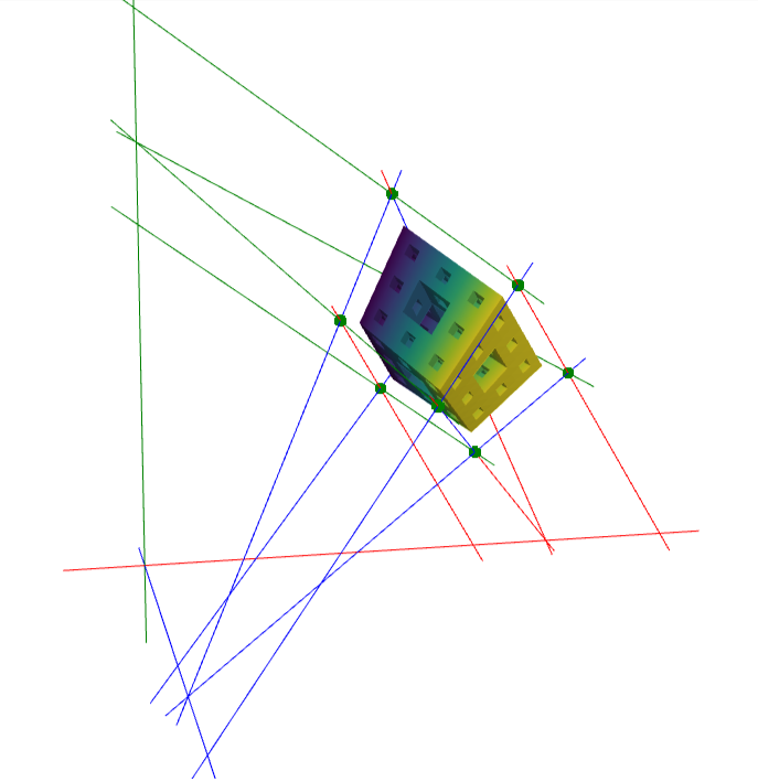
Figure 3: Left: the unit cube enclosing a model. Middle: deformation of the unit cube and the model using the trilinear rational map constructed in Example 6.2, with uniform weights $w_{ijk}=1$ for every $0\leq i,j,k\leq 1$. Right: the lines $s$ (red), $t$ (green), and $u$ (blue) used in the construction. These three lines intersect at a common point. Additionally, all the boundary $s$-lines (red), $t$-lines (green), and $u$-lines respectively intersect $s,t$, and $u$.

In particular, the boundary surfaces are smooth quadrics. Hence, these control points produce a “quadcube”, i.e. a quadrilateral-faced hexahedron where the flat facets are replaced by quadric surfaces.

6.2 Birational weights and tensor rank criterion

Let $\phi$ be tripod. We denote by $\Pi_{1}$ (resp. $\Pi_{2}$ and $\Pi_{3}$) the plane through $t,u$ (resp. $s,u$ and $s,t$), which is defined by $\pi_{r}=\boldsymbol{\pi}_{r}\cdot\mathbf{x}^{T}$ for $r=1$ (resp. $r=2$ and $r=3$) and some $\boldsymbol{\pi}_{r}$ in $\mathbb{R}^{4}$. Additionally, for each $0\leq i,j,k\leq 1$, we define

$$\Delta_{ijk}(r)=\frac{1}{\langle\boldsymbol{\pi}_{r},\mathbf{P}_{ijk}\rangle}\ .$$

Remark 6.3.

For tripod maps, $\Delta_{ijk}(r)$ is well-defined for every $0\leq i,j,k\leq 1$ and $r=1,2,3$. Specifically, $\Delta_{ijk}(r)$ is not well-defined if and only if $\mathbf{P}_{ijk}$ lies on the plane $\Pi_{r}$. Without loss of generality, let $r=1$. Then, the boundary line $t_{ik}$ (resp. $u_{ij}$) also lies in $\Pi_{1}$, since it intersects $t$ (resp. $u$) and $\Pi_{1}=\text{Plane}(t,u)$. Similarly, the control point $\mathbf{P}_{ij^{*}k}$ (resp. $\mathbf{P}_{ijk^{*}}$) lies in $\Pi_{1}$, and the line $u_{ij^{*}}$ (resp. $t_{ik^{*}}$) as well for the same reasons as before. Therefore, the four control points $\mathbf{P}_{i00},\mathbf{P}_{i10},\mathbf{P}_{i01}$, and $\mathbf{P}_{i11}$ are coplanar, yielding a contradiction with the fact that $\Sigma_{i}$ is a smooth quadric.

As in § 3.2, § 4.2, and § 5.2, the birationality of a tripod map is equivalent to a rank-one condition on a $2\times 2\times 2$ tensor.

Let $\phi$ be tripod. The following are equivalent:

1. $\phi$ is birational of type $(2,2,2)$

2. One of the three tensors

   $$W(r)=\left(\frac{w_{ijk}}{\Delta_{ijk}(r)}\right)_{0\leq i,j,k\leq 1}$$

   for each $r=1,2,3$, has rank one

3. The three tensors above have rank one

Proof 6.4.

First, we prove that 1 implies both 2 and 3. The tensor $W(r)$ encodes the coefficients of the trilinear polynomial

$$\langle\boldsymbol{\pi}_{r},\mathbf{f}\rangle=\sum_{0\leq i,j,k\leq 1}w_{ijk}\,\langle\boldsymbol{\pi}_{r},\mathbf{P}_{ijk}\rangle\,s_{i}t_{j}u_{k}=\sum_{0\leq i,j,k\leq 1}\left(\frac{w_{ijk}}{\Delta_{ijk}(r)}\right)\,s_{i}t_{j}u_{k}$$

for each $r=1,2,3$. In particular, $\langle\boldsymbol{\pi}_{r},\mathbf{f}\rangle=0$ defines the pullback by $\phi$ of the plane $\Pi_{r}$. By § 6.1, the lines $s,t$, and $u$ are components of the base locus of $\phi^{-1}$. Hence, $\phi$ contracts some surfaces in $\mathbb{P}^{3}$ to each of them. Since, $\Pi_{1}=\text{Plane}(t,u)$, $\Pi_{2}=\text{Plane}(s,u)$, and $\Pi_{3}=\text{Plane}(s,t)$ we find two factors on $\langle\boldsymbol{\pi}_{r},\mathbf{f}\rangle$, for each $r=1,2,3$. Equivalently, the tensor $W(r)$ has rank one.

We continue proving that $2$ implies $3$. Without loss of generality, we assume that

$$W(1)=\left(\alpha_{i0}\,\beta_{j1}\,\gamma_{k1}\right)_{0\leq i,j,k\leq 1}$$

for some $(\alpha_{00}:\alpha_{10})\times(\beta_{01}:\beta_{11})\times(\gamma_{01}:\gamma_{11})$ in $(\mathbb{P}{R}^{1})^{3}$. In particular, we find the factorization

(34) $$\langle\boldsymbol{\pi}_{1},\mathbf{f}\rangle=\sum_{0\leq i,j,k\leq 1}\left(\frac{w_{ijk}}{\Delta_{ijk}(1)}\right)s_{i}t_{j}u_{k}=\sum_{0\leq i,j,k\leq 1}(\alpha_{i0}s_{i})(\beta_{j1}t_{j})(\gamma_{k1}u_{k})=a_{0}b_{1}c_{1}\ ,$$

where

(35) $$a_{0}(s_{0},s_{1})=\begin{vmatrix}\phantom{-}s_{0}&s_{1}\\ -\alpha_{10}&\alpha_{00}\end{vmatrix}\ \ ,\ \ b_{1}(t_{0},t_{1})=\begin{vmatrix}\phantom{-}t_{0}&t_{1}\\ -\beta_{11}&\beta_{01}\end{vmatrix}\ \ ,\ \ c_{1}(u_{0},u_{1})=\begin{vmatrix}\phantom{-}u_{0}&u_{1}\\ -\gamma_{11}&\gamma_{01}\end{vmatrix}\ .$$

Therefore, the images by $\phi$ of the surfaces defined by $a_{0}=0$, $b_{1}=0$, and $c_{1}=0$ lie in $\Pi_{1}$. We make the following observations:

1. Since $\phi$ is tripod, the four boundary $t$-lines (resp. $u$-lines) meet $\Pi_{1}$ at the line $t$ (resp. $u$). Hence, $\phi$ contracts $b_{1}=0$ (resp. $c_{1}=0$) to $t$ (resp. $u$)

2. The image of $a_{0}=0$ is dense in $\Pi_{1}$

Now, for each $0\leq i,j,k\leq 1$ consider the line isomorphisms $\phi_{jk}:\mathbb{P}^{1}\xrightarrow{}s_{jk}\subset\mathbb{P}^{3}$ defined by $\mathbf{P}_{jk}(s_{0},s_{1})=w_{0jk}\,\mathbf{P}_{0jk}\,s_{0}+w_{1jk}\,\mathbf{P}_{1jk}\,s_{1}$, as well as the planes

$$T_{ik}=\text{Plane}(t,t_{ik})\equiv\tau_{ik}=0\ ,\ Y_{ij}=\text{Plane}(u,u_{ij})\equiv\upsilon_{ij}=0$$

for some linear forms $\tau_{ik}$ and $\upsilon_{ij}$ in $\mathbb{R}[x_{0},x_{1},x_{2},x_{3}]$. By the second observation above, $\phi_{jk}$ is the unique isomorphism sending

$$(1:0)\mapsto\mathbf{P}_{0jk}\ ,\ (0:1)\mapsto\mathbf{P}_{1jk}\ ,\ (-\alpha_{10}:\alpha_{00})\mapsto s_{jk}\cap\Pi_{1}\ .$$

Additionally, define the line isomorphisms

$$\theta_{k}:\mathbb{P}^{1}\xrightarrow{}(\mathbb{P}^{3})^{\vee}\ :\ (s_{0}:s_{1})=(1:0)\mapsto\tau_{0k}\ ,\ (s_{0}:s_{1})=(0:1)\mapsto\tau_{1k}\ ,\ (s_{0}:s_{1})=(-\alpha_{10}:\alpha_{00})\mapsto\pi_{1}\ ,$$

$$\rho_{j}:\mathbb{P}^{1}\xrightarrow{}(\mathbb{P}^{3})^{\vee}\ :\ (s_{0}:s_{1})=(1:0)\mapsto\upsilon_{0j}\ ,\ (s_{0}:s_{1})=(0:1)\mapsto\upsilon_{1j}\ ,\ (s_{0}:s_{1})=(-\alpha_{10}:\alpha_{00})\mapsto\pi_{1}\ .$$

In particular, $\theta_{k}$ and $\rho_{j}$ parametrize the pencils of planes respectively defined by the lines $t$ and $u$. Let $\boldsymbol{\theta}_{k}=\boldsymbol{\theta}_{k}(s_{0},s_{1})$ and $\boldsymbol{\rho}_{j}=\boldsymbol{\rho}_{j}(s_{0},s_{1})$ be tuples in $(\mathbb{R}[s_{0},s_{1}]_{1})^{4}$ of linear polynomials respectively defining these two parametrizations. Hence, we find

$$\langle\boldsymbol{\theta}_{k},\mathbf{P}_{jk}\rangle=0\ ,\ \langle\boldsymbol{\rho}_{j},\mathbf{P}_{jk}\rangle=0\ .$$

More explicitly, the scalar products above are either identically zero or quadratic homogeneous polynomials in $s_{0},s_{1}$ vanishing at the three points $(1:0),(0:1)$ and $(-\alpha_{10}:\alpha_{00})$, hence identically zero. Therefore, $\boldsymbol{\theta}_{k}$ and $\boldsymbol{\rho}_{j}$ define syzygies of $\mathbb{Z}^{3}$-degree $(1,0,0)$ of $\mathbf{P}_{jk}$. On the other hand, since $\Pi_{2}=\text{Plane}(s,u)$ and $\Pi_{3}=\text{Plane}(s,t)$, it follows that the three conditions:

1. $\mathbf{P}_{jk}(s_{0},s_{1})=s_{jk}\cap s=s_{jk}\cap\Pi_{2}=s_{jk}\cap\Pi_{3}$

2. $\boldsymbol{\theta}_{k}(s_{0},s_{1})=\boldsymbol{\pi}_{3}$

3. $\boldsymbol{\rho}_{j}(s_{0},s_{1})=\boldsymbol{\pi}_{2}$

are equivalent. Now, define

$$a_{1}(s_{0},s_{1})=\begin{vmatrix}s_{0}&s_{1}\\ -\alpha_{11}&\alpha_{01}\end{vmatrix}$$

such that $\mathbf{P}_{00}(\alpha_{01},\alpha_{11})=s_{00}\cap s$. By the former equivalences, we find $\theta_{0}(\alpha_{01},\alpha_{11})=\pi_{3}$ and $\rho_{0}(\alpha_{01},\alpha_{11})=\pi_{2}$. Similarly, these imply

$$\mathbf{P}_{10}(\alpha_{01},\alpha_{11})=s_{10}\cap s\ ,\ \mathbf{P}_{01}(\alpha_{01},\alpha_{11})=s_{01}\cap s\ ,$$

which again yield $\theta_{1}(\alpha_{01},\alpha_{11})=\pi_{3}$ and $\rho_{1}(\alpha_{01},\alpha_{11})=\pi_{2}$, and thus $\mathbf{P}_{11}(\alpha_{01},\alpha_{11})=s_{11}\cap s$. Therefore, since $\mathbf{P}_{jk}(\alpha_{01},\alpha_{11})$ lies in the line $s$ for every $0\leq j,k\leq 1$, it follows that $\phi$ contracts the surface $a_{1}=0$ to $s$. Furthermore, this readily implies

(36) $$\langle\boldsymbol{\pi}_{2},\mathbf{f}\rangle=\sum_{0\leq i,j,k\leq 1}\left(\frac{w_{ijk}}{\Delta_{ijk}(2)}\right)s_{i}t_{j}u_{k}=a_{1}b_{0}c_{1}\ \ ,\ \ \langle\boldsymbol{\pi}_{3},\mathbf{f}\rangle=\sum_{0\leq i,j,k\leq 1}\left(\frac{w_{ijk}}{\Delta_{ijk}(3)}\right)s_{i}t_{j}u_{k}=a_{1}b_{1}c_{0}\ ,$$

for some

(37) $$b_{0}(t_{0},t_{1})=\begin{vmatrix}t_{0}&t_{1}\\ -\beta_{10}&\beta_{00}\end{vmatrix}\ \ ,\ \ c_{0}(u_{0},u_{1})=\begin{vmatrix}u_{0}&u_{1}\\ -\gamma_{10}&\gamma_{00}\end{vmatrix}\ \ ,$$

and 3 follows.

We conclude proving that 3 implies 1. Since $\phi$ is tripod, we have the intersections

$$\Sigma_{0}\cap\Sigma_{1}=t\cup u\cup C\ ,\ T_{0}\cap T_{1}=s\cup u\cup C\ ,\ Y_{0}\cap Y_{1}=s\cup t\cup C\ .$$

In particular, the cone $Q$ of apex $\mathbf{A}=s\cap t\cap u$ through the plane conic $C$ is a linear combination of the two boundary surfaces for each of the three parameters. Similarly, the rank-two quadrics

$$\Pi_{1}\cup\Pi\ ,\ \Pi_{2}\cup\Pi\ ,\ \Pi_{3}\cup\Pi$$

are also linear combinations of the boundary surfaces respectively for the first, second, and third parameters. Thus, we can write

(38) $$\begin{pmatrix}\phantom{-}\lambda_{11}&-\lambda_{01}\\ -\lambda_{10}&\phantom{-}\lambda_{00}\end{pmatrix}\begin{pmatrix}\pi_{1}\pi\\ q\end{pmatrix}=\begin{pmatrix}\sigma_{0}\\ \sigma_{1}\end{pmatrix}\ ,\ \begin{pmatrix}\phantom{-}\mu_{11}&-\mu_{01}\\ -\mu_{10}&\phantom{-}\mu_{00}\end{pmatrix}\begin{pmatrix}\pi_{2}\pi\\ q\end{pmatrix}=\begin{pmatrix}\tau_{0}\\ \tau_{1}\end{pmatrix}\ ,\ \begin{pmatrix}\phantom{-}\nu_{11}&-\nu_{01}\\ -\nu_{10}&\phantom{-}\nu_{00}\end{pmatrix}\begin{pmatrix}\pi_{3}\pi\\ q\end{pmatrix}=\begin{pmatrix}\upsilon_{0}\\ \upsilon_{1}\end{pmatrix}$$

for some $\lambda_{ij},\mu_{ij},\nu_{ij}$ yielding invertible matrices. Additionally, by § 2.1 all these coefficients are nonzero since the boundary surfaces are smooth. Let $\varphi_{1}:\mathbb{P}^{1}\xrightarrow{}\left(\mathbb{P}^{9}\right)^{\vee}\simeq\mathbb{P}(\mathbb{C}[x_{0},x_{1},x_{2},x_{3}]_{2})$ be the line isomorphism defined by

$$(\zeta_{0}:\zeta_{1})\mapsto\begin{vmatrix}\zeta_{0}&\zeta_{1}\\ \pi_{1}\pi&q\end{vmatrix}\ ,$$

whose image is the line $L_{1}$ spanned by $\pi_{1}\pi$ and $q$ in the space of quadrics in $\mathbb{P}^{3}$. By Eq. 38, $\sigma_{0},\sigma_{1}$ belong to $L_{1}$. Furthermore, by hypothesis we find the factorizations

$$\pi_{1}(f_{0},f_{1},f_{2},f_{3})=\langle\boldsymbol{\pi}_{1},\mathbf{f}\rangle=a_{0}b_{1}c_{1}\ ,\ q(f_{0},f_{1},f_{2},f_{3})=a_{1}b_{1}c_{1}h_{1}$$

for some trilinear $h_{1}=h_{1}(s_{0},s_{1},t_{0},t_{1},u_{0},u_{1})$. Then, $\varphi_{1}$ induces a second line isomorphim $\varphi_{1}^{\prime}$ from $\mathbb{P}^{1}$ to a line $L_{1}^{\prime}$ in the space of polynomials of $\mathbb{Z}^{3}$-degree $(2,2,2)$, defined by

$$(\zeta_{0}:\zeta_{1})\mapsto\begin{vmatrix}\zeta_{0}&\zeta_{1}\\ a_{0}b_{1}c_{1}h_{0}&a_{1}b_{1}c_{1}h_{1}\end{vmatrix}=b_{1}c_{1}\begin{vmatrix}\zeta_{0}&\zeta_{1}\\ a_{0}h_{0}&a_{1}h_{1}\end{vmatrix}$$

where $h_{0}=\pi(f_{0},f_{1},f_{2},f_{3})=\langle\boldsymbol{\pi},\mathbf{f}\rangle$. In particular, $L_{1}^{\prime}$ can be realized in the projective space of homogeneous polynomials of $\mathbb{Z}^{3}$-degree $(2,1,1)$ as the line spanned by $a_{0}h_{0}$ and $a_{1}h_{1}$. On the other hand, the locus of polynomials admitting a factorization of the form

$$g_{0}(s_{0},s_{1})\,g_{1}(s_{0},s_{1},t_{0},t_{1},u_{0},u_{1})\ ,$$

with $g_{0},g_{1}$ respectively of $\mathbb{Z}^{3}$-degrees $(1,0,0)$ and $(1,1,1)$, is cut out by quadratic equations. Therefore, $L_{1}^{\prime}$ is either contained in this locus or intersects it in at most two points. However, $L_{1}^{\prime}$ contains the four distinct points

$$a_{0}h_{0}\ ,\ a_{1}h_{1}\ ,\ b_{1}^{-1}c_{1}^{-1}\sigma_{0}(f_{0},f_{1},f_{2},f_{3})=s_{0}h_{0}^{\prime}\ ,\ b_{1}^{-1}c_{1}^{-1}\sigma_{1}(f_{0},f_{1},f_{2},f_{3})=s_{1}h_{1}^{\prime}\ ,$$

for some trilinear $h_{i}^{\prime}=h_{i}^{\prime}(s_{0},s_{1},t_{0},t_{1},u_{0},u_{1})$. Hence, all the points in $L_{1}^{\prime}$ factor as above, and $\varphi_{1}^{\prime}:\mathbb{P}^{1}\xrightarrow{}L_{1}^{\prime}$ can be written as

$$(\zeta_{0}:\zeta_{1})\mapsto\begin{vmatrix}\zeta_{0}&\zeta_{1}\\ a_{0}h&a_{1}h\end{vmatrix}=h\begin{vmatrix}\zeta_{0}&\zeta_{1}\\ a_{0}&a_{1}\end{vmatrix}$$

for some trilinear $h=h(s_{0},s_{1},t_{0},t_{1},u_{0},u_{1})$. In particular, the rational map $\phi_{1}:\mathbb{P}^{3}\dashrightarrow\mathbb{P}^{1}$ defined by

$$(x_{0}:x_{1}:x_{2}:x_{3})\mapsto(A_{0}:A_{1})=(\alpha_{11}\,\pi_{1}\pi-\alpha_{10}\,q:-\alpha_{01}\,\pi_{1}\pi+\alpha_{00}\,q)$$

yields the inverse of $\phi$ on the first $\mathbb{P}^{1}$ factor of $(\mathbb{P}^{1})^{3}$, since

$$\mathbb{R}[x_{0},x_{1},x_{2},x_{3}]^{2}\ni(A_{0},A_{1})\xmapsto{x_{i}\mapsto f_{i}}b_{1}c_{1}h\,(s_{0},s_{1})\in R^{2}\ .$$

With parallel arguments, we derive the inverse for the remaining two factors of $(\mathbb{P}^{1})^{3}$. Hence, $\phi$ is birational of type $(2,2,2)$.

Let $\phi$ be tripod. Then, $\phi$ is birational of type $(2,2,2)$ if and only if one, and therefore all, of the following conditions:

1. $w_{ijk}=\alpha_{i0}\,\beta_{j1}\,\gamma_{k1}\,\Delta_{ijk}(1)$ for each $0\leq i,j,k\leq 1$

2. $w_{ijk}=\alpha_{i1}\,\beta_{j0}\,\gamma_{k1}\,\Delta_{ijk}(2)$ for each $0\leq i,j,k\leq 1$

3. $w_{ijk}=\alpha_{i1}\,\beta_{j1}\,\gamma_{k0}\,\Delta_{ijk}(3)$ for each $0\leq i,j,k\leq 1$

holds for some $(\alpha_{0i}:\alpha_{1i})$, $(\gamma_{0j}:\beta_{1j})$, and $(\gamma_{0k}:\gamma_{1k})$ in $\mathbb{P}{R}^{1}$, up to a nonzero scalar multiplying all the weights.

6.2.1 The contractions of a tripod birational map

Let $\phi$ be tripod with weights as in § 6.2. In particular, $\phi$ is birational of type $(2,2,2)$, and by § 6.1 we have the following:

1. The rank-two quadric $\Pi\cup\Pi_{1}$ (resp. $\Pi\cup\Pi_{2}$ and $\Pi\cup\Pi_{3}$) belongs to the pencil of $s$-surfaces (resp. $t$- and $u$-surfaces). Namely, we find $(\lambda_{00}:\lambda_{10})$ (resp. $(\mu_{00}:\mu_{10})$ and $(\nu_{00}:\nu_{10})$) in $\mathbb{P}{R}^{1}$ such that $\Pi\cup\Pi_{1}$ (resp. $\Pi\cup\Pi_{2}$ and $\Pi\cup\Pi_{3}$) is defined by

   $$\lambda_{00}\,\sigma_{0}+\lambda_{10}\,\sigma_{1}=0\ \ \text{(resp}.\text{\ }\mu_{00}\,\tau_{0}+\mu_{10}\,\tau_{1}=0\ \text{ and }\ \nu_{00}\,\upsilon_{0}+\nu_{10}\,\upsilon_{1}=0\text{)}$$

2. The cone $Q$ of apex $\mathbf{A}$ through the plane conic $C$ belongs to the pencils of $s$-, $t$-, and $u$-surfaces. In particular, $Q$ is defined by a quadratic form $q=q(\mathbf{x})$, and we find points $(\lambda_{01}:\lambda_{11}),(\mu_{01}:\mu_{11})$, and $(\nu_{01}:\nu_{11})$ in $\mathbb{P}{R}^{1}$ such that

   $$q=\lambda_{01}\,\sigma_{0}+\lambda_{11}\,\sigma_{1}=\mu_{01}\,\tau_{0}+\mu_{11}\,\tau_{1}=\nu_{01}\,\upsilon_{0}+\nu_{11}\,\upsilon_{1}$$

As for the previous classes of birational maps, § 6.2 readily implies the following corollary.

Let $\phi$ be tripod with weights as in § 6.2, and let

(39) $$a_{i}(s_{0},s_{1})=\begin{vmatrix}\phantom{-}s_{0}&s_{1}\\ -\alpha_{1i}&\alpha_{0i}\end{vmatrix}\ \ ,\ \ b_{j}(t_{0},t_{1})=\begin{vmatrix}\phantom{-}t_{0}&t_{1}\\ -\beta_{1j}&\beta_{0j}\end{vmatrix}\ \ ,\ \ c_{k}(u_{0},u_{1})=\begin{vmatrix}\phantom{-}u_{0}&u_{1}\\ -\gamma_{1k}&\gamma_{0k}\end{vmatrix}$$

for each $0\leq i,j,k\leq 1$, as well as

$$h(s_{0},s_{1},t_{0},t_{1},u_{0},u_{1})=\omega_{1}\,a_{0}b_{1}c_{1}+\omega_{2}\,a_{1}b_{0}c_{1}+\omega_{3}\,a_{1}b_{1}c_{0}$$

for some $\omega_{1},\omega_{2},\omega_{3}$ in $\mathbb{R}$ such that $q=\omega_{1}\,\pi_{2}\pi_{3}+\omega_{2}\,\pi_{1}\pi_{3}+\omega_{3}\,\pi_{1}\pi_{2}$. Then, we have the following:

1. $\phi$ contracts the surface $a_{1}=0$ to the line $s$

2. $\phi$ contracts the surface $b_{1}=0$ to the line $t$

3. $\phi$ contracts the surface $c_{1}=0$ to the line $u$

4. $\phi$ contracts the surface $h=0$ to the plane conic $C$

5. The image of the surface $a_{0}=0$ is dense in the plane $\Pi_{1}$

6. The image of the surface $b_{0}=0$ is dense in the plane $\Pi_{2}$

7. The image of the surface $c_{0}=0$ is dense in the plane $\Pi_{3}$

Proof 6.5.

Follows from the proof of § 6.2. In particular, the cone $Q$ of apex $\mathbf{A}=s\cap t\cap u$ through the plane conic $C$ is defined by $q=\omega_{1}\,\pi_{2}\pi_{3}+\omega_{2}\,\pi_{1}\pi_{3}+\omega_{3}\,\pi_{1}\pi_{2}$. Since $\phi$ contracts the surfaces $a_{1}=0$, $b_{1}=0$, and $c_{1}=0$ respectively to the lines $s,t$, and $u$, we find the factorization

$$q(f_{0},f_{1},f_{2},f_{3})=a_{1}b_{1}c_{1}\,(\omega_{1}\,a_{1}b_{0}c_{0}+\omega_{2}\,a_{0}b_{1}c_{0}+\omega_{3}\,a_{0}b_{0}c_{1})=a_{1}b_{1}c_{1}h\ .$$

By the proof of 3 implies 1 in § 6.2, the image of $h=0$ lies on the plane $\Pi$. Hence, $\phi$ contracts $h=0$ to $C=\Pi\cap Q$.

6.3 Inverse and base locus

As in § 3.3, § 4.3, and § 5.3, we close the section giving explicit formulas for the inverse of a tripod birational map.

Let $\phi$ be tripod with weights as in § 6.2. Then, $\phi^{-1}$ is given by

$$(x_{0}:x_{1}:x_{2}:x_{3})\mapsto\left(\alpha_{1i}\,\lambda_{1i}\,\sigma_{1}:\alpha_{0i}\,\lambda_{0i}\,\sigma_{0}\right)\times\left(\beta_{1j}\,\mu_{1j}\,\tau_{1}:\beta_{0j}\,\mu_{0j}\,\tau_{0}\right)\times\left(\gamma_{1k}\,\nu_{1k}\,\upsilon_{1}:\gamma_{0k}\,\nu_{0k}\,\upsilon_{0}\right)\ ,$$

where any $0\leq i,j,k\leq 1$ are valid. Additionally, with the notation of § 6.2.1, we have the following:

1. The base locus of $\phi$ is defined by the ideal

   (40) $$I:\mathfrak{N}^{\infty}=(a_{0},b_{0},c_{0})\cap(a_{1}^{2},b_{1}^{2},c_{1}^{2},a_{1}b_{1},a_{1}c_{1},b_{1}c_{1},\omega_{1}\,a_{1}b_{0}c_{0}+\omega_{2}\,a_{0}b_{1}c_{0}+\omega_{3}\,a_{0}b_{0}c_{1})$$

2. The base locus of $\phi^{-1}$ is $s\cup t\cup u\cup C$

3. $\phi$ blows up the base point $(a_{0},b_{0},c_{0})$ to the plane $\Pi$

4. $\phi$ blows up the nonreduced base point $(a_{1},b_{1},c_{1})$ to the cone $Q$

Proof 6.6.

By § 6.2, $\phi$ is birational of type $(2,2,2)$. As explained in the proofs of § 4.3 and § 5.3, the inverses on each factor of $(\mathbb{P}^{1})^{3}$ can be regarded as line isomorphisms $\sigma,\tau,\upsilon:\mathbb{P}^{1}\xrightarrow{}(\mathbb{P}^{9})^{\vee}$, to the space $(\mathbb{P}^{9})^{\vee}$ of quadrics in $\mathbb{P}^{3}$, satisfying

$$\sigma:(1:0)\mapsto\sigma_{0}\ ,\ (0:1)\mapsto\sigma_{1}\ ,\ \tau:(1:0)\mapsto\tau_{0}\ ,\ (0:1)\mapsto\tau_{1}\ ,\ \upsilon:(1:0)\mapsto\upsilon_{0}\ ,\ (0:1)\mapsto\upsilon_{1}\ .$$

By § 6.2.1, $\phi$ contracts the surface $a_{1}=0$ (resp. $b_{1}=0$ and $c_{1}=0$) to the line $s\subset Q$ (resp. $t\subset Q$ and $u\subset Q$). On the other hand, $\phi$ also maps the surface $a_{0}=0$ (resp. $b_{0}=0$ and $c_{0}=0$) to the plane $\Pi_{1}$ (resp. $\Pi_{2}$ and $\Pi_{3}$). These two observations readily imply

$$\sigma:(-\alpha_{10}:\alpha_{00})\mapsto\pi_{1}\pi\ ,\ (-\alpha_{11}:\alpha_{01})\mapsto q$$

since $\Pi_{1}\cup\Pi$ and $Q$ are the quadrics in the pencil of $s$-surfaces respectively containing the plane $\Pi_{1}$ and the line $s$. Hence, $\sigma:\mathbb{P}^{1}\xrightarrow{}(\mathbb{P}^{9})^{\vee}$ is explicitly given by

$$(s_{0}:s_{1})\mapsto\begin{vmatrix}s_{0}&s_{1}\\ \alpha_{1i}\,\lambda_{1i}\,\sigma_{1}&\alpha_{0i}\,\lambda_{0i}\,\sigma_{0}\end{vmatrix}$$

where both $i=0,1$ are admissible. Similarly, we find

$$\tau:(t_{0}:t_{1})\mapsto\begin{vmatrix}t_{0}&t_{1}\\ \beta_{1j}\,\mu_{1j}\,\tau_{1}&\beta_{0j}\,\mu_{0j}\,\tau_{0}\end{vmatrix}\ \ ,\ \ \upsilon:(u_{0}:u_{1})\mapsto\begin{vmatrix}s_{0}&s_{1}\\ \gamma_{1k}\,\nu_{1k}\,\gamma_{1}&\gamma_{0k}\,\nu_{0k}\,\gamma_{0}\end{vmatrix}$$

for any $0\leq j,k\leq 1$, and $\phi^{-1}$ is as in the statement.

The base locus of $\phi^{-1}$ follows immediately from § 6.1. On the other hand, we have the identity

$${I^{\prime}}_{(1,1,1)}=\mathbb{R}\langle a_{0}b_{1}c_{1},a_{1}b_{0}c_{1},a_{1}b_{1}c_{0},h\rangle=\mathbb{R}\langle\langle\boldsymbol{\pi}_{1},\mathbf{f}\rangle,\langle\boldsymbol{\pi}_{2},\mathbf{f}\rangle,\langle\boldsymbol{\pi}_{3},\mathbf{f}\rangle,\langle\boldsymbol{\pi},\mathbf{f}\rangle\rangle=\mathbb{R}\langle f_{0},f_{1},f_{2},f_{3}\rangle$$

where $I^{\prime}$ is the ideal on the right-hand side of Eq. 40, which is saturated. Hence, $I^{\prime}$ defines the base locus of $\phi$. The blow-ups follow from the proof of § 6.1.

7 Effective manipulation of birational trilinear volumes

We conclude the paper introducing several effective methods for approximating and manipulating birational trilinear volumes. They rely on the results of the previous sections, and exploit the connection between birationality and tensor rank. We illustrate these methods through several examples, that emphasize how they are meaningful for applications.

7.1 Distance to birationality

First we address Question 1.3, namely the poblem of measuring how “far” is a trilinear rational map from being birational. The intuition behind this question is clear, but the question itself lacks precision. To formalize it, the first step is to introduce a notion of distance that provides a precise definition of the term “far”.

Let $\mathfrak{Rat}_{(1,1,1)}$ denote the space of trilinear rational maps, and let $\mathfrak{Bir}_{(1,1,1)}\subset\mathfrak{Rat}_{(1,1,1)}$ be the locus of birational maps. In full generality, measuring the distance from $\phi$ to $\mathfrak{Bir}_{(1,1,1)}$ presents a delicate challenge. The first complication arises from the high dimensionality, since a trilinear rational map is determined by $31$ independent parameters (in the monomial basis: $8\times 4$ coefficients up to scalar; in the Bernstein basis: $3$ coordinates $\times$ $8$ control points + $8$ weights up to scalar) and hence $\mathfrak{Rat}_{(1,1,1)}\cong\mathbb{P}^{31}$. Secondly, by [6, Theorem 4.1] $\mathfrak{Bir}_{(1,1,1)}$ has eight irreducible components of various dimensions, and the distance from $\phi$ to each of the components is in general different.

Interestingly, § 3.2, § 4.2, § 5.2, and § 6.2 provide a way to quantify this distance. Specifically, since birationality is characterized by means of a rank-one condition on a $2\times 2\times 2$ tensor, we rely on the Frobenius norm for tensors [33] to define our notion of “distance to birationality”. Namely, it is the relative distance from the tensor $W$ that governs birationality to the locus of rank-one tensors, i.e. the affine cone over the Segre embedding of $\mathbb{P}{R}^{1}\times\mathbb{P}{R}^{1}\times\mathbb{P}{R}^{1}$.

Let $\phi$ be either hexahedral, pyramidal, scaffold, or tripod. Let $W$ be any of the tensors characterizing birationality (in the statements of § 3.2, § 4.2, § 5.2, and § 6.2) for the corresponding class. We define the distance to birationality of $\phi$, denoted by $\text{dist}_{\text{bir}}(\phi)$, as

(41) $$\text{dist}_{\text{bir}}(\phi)\coloneqq\min_{P\in V}\frac{\lVert W-P\rVert}{\lVert W\rVert}\ ,$$

where $V$ is the affine cone over the Segre embedding of $\mathbb{P}{R}^{1}\times\mathbb{P}{R}^{1}\times\mathbb{P}{R}^{1}$.

Remark 7.1.

The following observations are important:

1. For scaffold and tripod maps, several choices for $W$ are possible. However, § 5.2 and § 6.2 assert that $\text{dist}_{\text{bir}}(\phi)=0$ represents the same condition for any choice.

2. $\text{dist}_{\text{bir}}(\phi)$ is well defined. More explicitly, altough the vectors of $w_{ijk}$’s and $\Delta_{ijk}$’s are defined up to a nonzero scalar, they yield proportional tensors. Hence, the relative distances coincide.

Remarkably, this distance depends solely on the weights of $\phi$ (8 parameters up to scalar). This is a design-oriented approach, since a designer will typically move the control points of a rational map but will rarely modify the weights. Within this formulation, a “closest birational map” refers to a point in $V$ that minimizes the distance to $W$. In particular, it is an orthogonal projection of $\phi$ onto $V$. For a general $\phi$, there are exactly $6$ such projections, where at least two of them are real. Equivalently, the Euclidean distance degree of $V$ is $6$ [22, Example 8.2].

7.2 Computation of a birational approximation

We now deal with Question 1.4. In order to compute a birational approximation of $\phi$, we can compute a rank-one tensor $W_{\text{bir}}$ such that $\text{dist}_{\text{bir}}(\phi)=\lVert W\rVert^{-1}\lVert W-W_{\text{bir}}\rVert$. Equivalently, we can solve the optimization problem

(42) $$\min_{\begin{subarray}{c}W_{\text{bir}}\end{subarray}}\frac{\lVert W-W_{\text{bir}}\rVert}{\lVert W\rVert}\text{ where }W_{\text{bir}}=\boldsymbol{\alpha}\otimes\boldsymbol{\beta}\otimes\boldsymbol{\gamma}\text{ for some }\boldsymbol{\alpha},\boldsymbol{\beta},\boldsymbol{\gamma}\text{ in }\mathbb{R}^{2}$$

There is an extensive body of work related to tensor rank and fixed-rank approximations to solve this problem. An important tool is the Canonical Polyadic Decomposition (CPD) (e.g. [16, 32, 30, 33]). We rely on it to efficiently compute rank-one approximations. The following example illustrates how our results can be applied in practice to compute birational approximations of trilinear rational maps.

Example 7.2 (Birational approximation of a pyramidal rational map).

Consider the trilinear rational map $\phi$ defined by the control points

$$\mathbf{P}_{000}=\begin{pmatrix}1,&-\frac{8}{5},&0,&1\end{pmatrix}\ ,\ \mathbf{P}_{100}=\begin{pmatrix}1,&0,&-\frac{9}{5},&\frac{1}{2}\end{pmatrix}\ ,\ \mathbf{P}_{010}=\begin{pmatrix}1,&0,&\frac{27}{20},&\frac{1}{2}\end{pmatrix}\ ,\ \mathbf{P}_{110}=\begin{pmatrix}1,&\frac{4}{5},&0,&1\end{pmatrix}\ ,$$

$$\mathbf{P}_{001}=\begin{pmatrix}1,&-\frac{11}{10},&0,&\frac{9}{4}\end{pmatrix}\ ,\ \mathbf{P}_{101}=\begin{pmatrix}1,&0,&-\frac{4}{5},&3\end{pmatrix}\ ,\ \mathbf{P}_{011}=\begin{pmatrix}1,&0,&\frac{3}{5},&3\end{pmatrix}\ ,\ \mathbf{P}_{111}=\begin{pmatrix}1,&\frac{11}{20},&0,&\frac{9}{4}\end{pmatrix}\ ,$$

and $w_{ijk}=1$ for every $0\leq i,j,k\leq 1$. Since the four boundary $u$-lines, i.e. $u_{ij}=\overline{\mathbf{P}_{ij0}\mathbf{P}_{ij1}}$ for each $0\leq i,j\leq 1$, meet at the point $\mathbf{A}=\begin{pmatrix}1,&0,&0,&5\end{pmatrix}$ it follows that $\phi$ is pyramidal. In particular, we compute (recall § 4.2)

$$\Delta_{000}=\frac{5}{6}\ ,\ \Delta_{100}=\frac{20}{21}\ ,\ \Delta_{010}=\frac{80}{63}\ ,\ \Delta_{110}=\frac{5}{3}\ ,\ \Delta_{001}=\frac{40}{33}\ ,\ \Delta_{101}=\frac{15}{7}\ ,\ \Delta_{011}=\frac{20}{7}\ ,\ \Delta_{111}=\frac{80}{33}\ .$$

Thus, the tensor

$$W=\left(\frac{w_{ijk}}{\Delta_{ijk}}\right)_{0\leq i,j,k\leq 1}=\left(\frac{1}{\Delta_{ijk}}\right)_{0\leq i,j,k\leq 1}$$

does not have rank one, and by § 4.2 $\phi$ is not birational. However, we can render $\phi$ birational by computing new weights using the formulas in § 4.2 for any choice of $(\alpha_{0}:\alpha_{1})\times(\beta_{0}:\beta_{1})\times(\gamma_{0}:\gamma_{1})\in(\mathbb{P}{R}^{1})^{3}$. Nevertheless, the new birational map $\phi$ might differ significantly from the original $\phi$ if we make a “bad” choice. A smarter idea is to compute a rank-one CP decomposition of $W$. Using the Python library TensorFox [19], we compute the rational rank-one approximation of $W$ given by

$$W_{\text{bir}}=\left(\alpha_{0}\,,\,\alpha_{1}\right)\otimes\left(\beta_{0}\,,\,\beta_{1}\right)\otimes\left(\gamma_{0}\,,\,\gamma_{1}\right)=\left(0.95\,,\,0.91\right)\otimes\left(1.06\,,\,0.78\right)\otimes\left(1.08\,,\,0.75\right)\ .$$

Specifically, this leads to the exact rational weights $w_{ijk}=\alpha_{i}\,\beta_{j}\,\gamma_{k}\,\Delta_{ijk}$ for each $0\leq i,j,k\leq 1$. Additionally, we compute

$$\text{dist}_{\text{bir}}(\phi)=\frac{\lVert W-W_{\text{bir}}\rVert}{\lVert W\rVert}\sim 0.2594\ .$$

In Figure 4, we present a comparison between the deformations resulting from the original rational map, with uniform weights $w_{ijk}=1$ for every $0\leq i,j,k\leq 1$, and its birational approximation, utilizing the new weights.

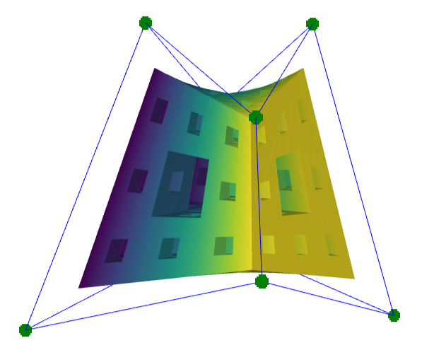
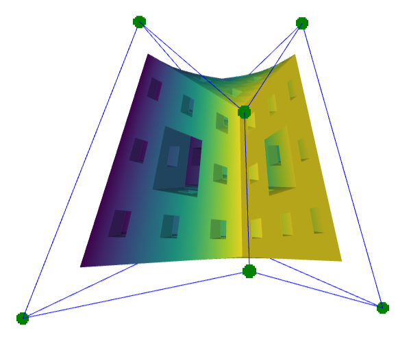
Figure 4: The two pyramidal maps presented in Example 7.2. In the left image, we use uniform weights, specifically $w_{ijk}=1$ for every $0\leq i,j,k\leq 1$. The right image showcases the effect of utilizing the computed birational weights. These weight adjustments subtly influence the deformation, while simultaneously ensuring the existence of an inverse transformation.

7.3 Exact computation of the inverse

§ 3.3, § 4.3, § 5.3, and § 6.3 provide explicit formulas for the inverse of a trilinear birational map, which are directly applicable in practice. The following example shows the explicit computation of the inverse of a pyramidal birational map.

Example 7.3.

We continue with Example 7.2, using the computed birational weights. In this case, the vectors and matrices defining the boundary surfaces are

$$\boldsymbol{\sigma}_{0}=\begin{pmatrix}5,&-\frac{5}{2},&\frac{10}{3},&1\end{pmatrix}\ \ ,\ \ \boldsymbol{\sigma}_{1}=\begin{pmatrix}4,&-4,&2,&-\frac{4}{5}\end{pmatrix}\ ,$$

$$\boldsymbol{\tau}_{0}=\begin{pmatrix}5,&\frac{5}{2},&\frac{5}{2},&-1\end{pmatrix}\ \ ,\ \ \boldsymbol{\tau}_{1}=\begin{pmatrix}-3,&3,&2,&\frac{3}{5}\end{pmatrix}\ ,$$

$$\boldsymbol{\upsilon}_{0}=\begin{pmatrix}390&-30&-\frac{45}{2}&-294\\[4.0pt] -30&75&0&60\\[4.0pt] -\frac{45}{2}&0&-50&\frac{45}{2}\\[4.0pt] -294&60&\frac{45}{2}&102\end{pmatrix}\ \ ,\ \ \boldsymbol{\upsilon}_{1}=\begin{pmatrix}1530&-\frac{495}{2}&-45&-438\\[4.0pt] -\frac{495}{2}&-225&0&\frac{165}{2}\\[4.0pt] -45&0&150&20\\[4.0pt] -438&\frac{165}{2}&20&114\end{pmatrix}\ .$$

Furthermore, using the formulas in § 4.2 we compute

$$(\lambda_{0}:\lambda_{1})\times(\mu_{0}:\mu_{1})\times(\nu_{0}:\nu_{1})=(4:-5)\times(3:-5)\times(11:-18)\ .$$

Thus, by § 4.3 $\phi^{-1}:\mathbb{P}{R}^{3}\dashrightarrow\mathbb{P}{R}^{1}\times\mathbb{P}{R}^{1}\times\mathbb{P}{R}^{1}$ is given by

$$(x_{0}:x_{1}:x_{2}:x_{3})\mapsto\left(\alpha_{1}\,\lambda_{1}\,\sigma_{1}:\alpha_{0}\,\lambda_{0}\,\sigma_{0}\right)\times\left(\beta_{1}\,\mu_{1}\,\tau_{1}:\beta_{0}\,\mu_{0}\,\tau_{0}\right)\times\left(\gamma_{1}\,\nu_{1}\,\upsilon_{1}:\gamma_{0}\,\nu_{0}\,\upsilon_{0}\right)\ .$$

7.4 Deformation of birational maps

An important task in the manipulation of birational transformations is the modification of the defining parameters, namely control points and weights, while preserving birationality. More specifically, we are interested in modifying these parameters continuously. This process is known as deformation, and it is instrumental in practice. Specifically, applications typically require the manipulation of the control points until the designer achieves the desired shape (e.g. [44, 43, 47, 48]).

Let $1\leq d_{1},d_{2},d_{3}\leq 2$, and let $\phi_{0},\phi_{1}$ be trilinear birational maps of type $(d_{1},d_{2},d_{3})$. Formally, a deformation of $\phi_{0}$ to $\phi_{1}$ is a continuous map $\delta:[0,1]\xrightarrow{}\mathcal{W}\times\mathcal{P}_{(d_{1},d_{2},d_{3})}$ (in the usual topology) such that $\delta(0)=\phi_{0}$ and $\delta(1)=\phi_{1}$, where $\mathcal{W}$ and $\mathcal{P}_{(d_{1},d_{2},d_{3})}$ are respectively the spaces of possible weights and control points for birational maps of type $(d_{1},d_{2},d_{3})$.

By Fact 1, § 4.1, § 5.1, and § 6.1 we can take $\mathcal{P}_{(d_{1},d_{2},d_{3})}$ as the set of configurations of control points $\{\mathbf{P}_{ijk}\}_{0\leq i,j,k\leq 1}$ that are either hexahedral, pyramidal, scaffold, or tripod. A small caveat is that pyramidal (resp. scaffold) birational maps can be of type either $(1,1,2)$, $(1,2,1)$, and $(2,1,1)$ (resp. $(1,2,2)$, $(2,1,2)$, and $(2,2,1)$), so the distinguished parameter should be specified. On the other hand, § 3.1, § 4.1, § 5.1, and § 6.1 provide effective methods for continuously manipulating the control points, while preserving the necessary constraints for birationality. Thus, they can be conveniently exploited for deformation. More explicitly, we can use the dominant rational parametrization of the irreducible component labelled by $(d_{1},d_{2},d_{3})$ (see [6, Theorem 4.1]) given by

(43) $$\Phi_{(d_{1},d_{2},d_{3})}:(\mathbb{P}{R}^{1})^{3}\times\mathcal{P}_{(d_{1},d_{2},d_{3})} \dasharrow \mathcal{W}\times\mathcal{P}_{(d_{1},d_{2},d_{3})}$$

$$(\alpha_{0}:\alpha_{1})\times(\beta_{0}:\beta_{1})\times(\gamma_{0}:\gamma_{1})\times(\ldots\,,\,\mathbf{P}_{ijk}\,,\,\ldots) \mapsto (\ldots:w_{ijk}:\ldots)\times(\ldots\,,\,\mathbf{P}_{ijk}\,,\,\ldots)=$$

$$(\ldots:\Delta_{ijk}\,\alpha_{i}\,\beta_{j}\,\gamma_{k}:\ldots)\times(\ldots\,,\,\mathbf{P}_{ijk}\,,\,\ldots)$$

In particular, by § 3.2, § 4.2, § 5.2, and § 6.2 for a fixed choice of control points, $\Phi_{(d_{1},d_{2},d_{3})}$ yields all the weights that render $\phi$ birational of type $(d_{1},d_{2},d_{3})$.

The previous parametrization explains how deformation can be performed. Specifically, a user can continuously decide new control points, and update the $\Delta_{ijk}$’s accordingly (which are continuous functions in the coordinates of the points) while keeping the same tensor decomposition $W=(\alpha_{0},\alpha_{1})\otimes(\beta_{0},\beta_{1})\otimes(\gamma_{0},\gamma_{1})$ for each instant $t\in[0,1]$ of the deformation, by applying the formulas $w_{ijk}=\alpha_{i}\,\beta_{j}\,\gamma_{k}\,\Delta_{ijk}$ for each $0\leq i,j,k\leq 1$.

The following is an example of the deformation of hexahedral birational maps. This case is particularly important in practice, since hexahedral meshes appear frequently in geometric modeling. Furthermore, the generation of the control points proposed in § 3.1 is simple and intuitive, making it appealing for applications.

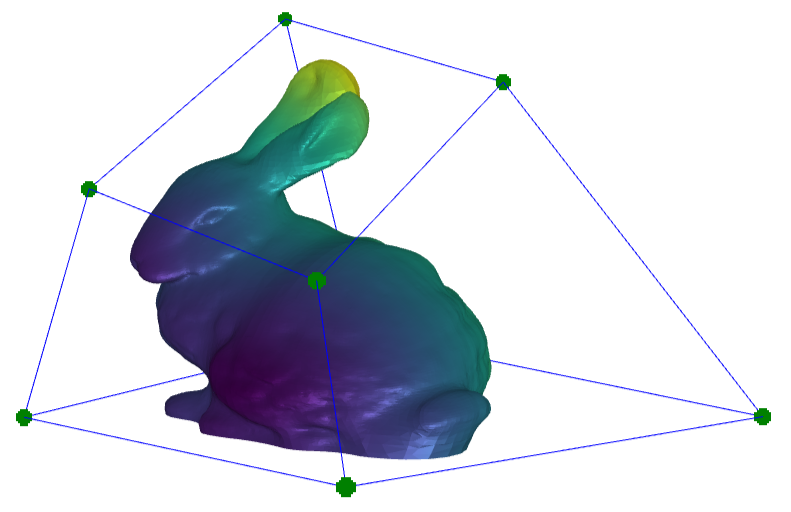
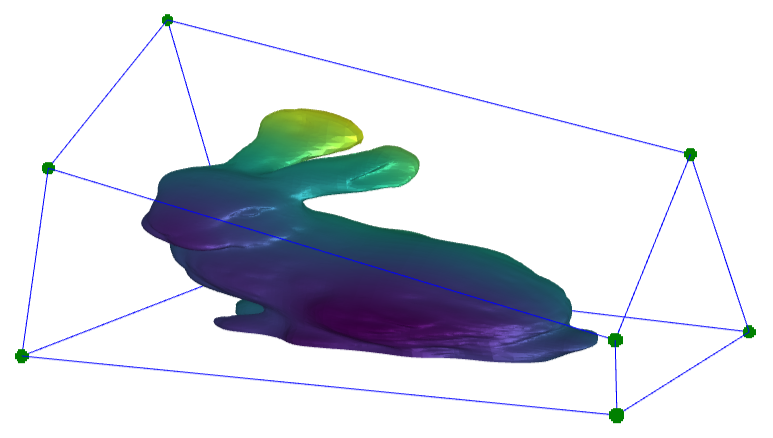
Figure 5: A birational deformation of the hexahedral birational map of Example 7.4. The boundary plane $\Sigma_{1}$, previously defined by the vector $\boldsymbol{\sigma}_{1}=(1.25,\,-0.63,\,-0.32,\,-0.63)$, is updated to the plane defined by $\boldsymbol{\sigma}_{1}=(2.31,\,-0.84,\,-0.2,\,-0.32)$, yielding new control points. Additionally, the weights are also updated to preserve birationality.

Example 7.4 (Deformation of a hexahedral birational map).

Consider the boundary planes defined by

$$\boldsymbol{\sigma}_{0}=\begin{pmatrix}0.16,&-0.45,&-0.07,&-0.14\end{pmatrix}\ \ ,\ \ \boldsymbol{\sigma}_{1}=\begin{pmatrix}1.25,&-0.63,&-0.32,&-0.63\end{pmatrix}\ ,$$

$$\boldsymbol{\tau}_{0}=\begin{pmatrix}0,&0,&0,&1\end{pmatrix}\ \ ,\ \ \boldsymbol{\tau}_{1}=\begin{pmatrix}-1.18,&0.18,&0.51,1\end{pmatrix}\ ,$$

$$\boldsymbol{\upsilon}_{0}=\begin{pmatrix}0,&0,&1,&0\end{pmatrix}\ \ ,\ \ \boldsymbol{\upsilon}_{1}=\begin{pmatrix}-1.17,&0.1,&0.8,&0.54\end{pmatrix}\ .$$

For each $0\leq i,j,k\leq 1$, we can use the formula Eq. 11 and express $\mathbf{P}_{ijk}=\Sigma_{i}\cap T_{j}\cap Y_{k}$ as the exterior product

(44) $$\mathbf{P}_{ijk}=\Delta_{ijk}^{-1}\ \boldsymbol{\sigma}_{i}\wedge\boldsymbol{\tau}_{j}\wedge\boldsymbol{\upsilon}_{k}\ ,$$

where each $\Delta_{ijk}$ can be computed using Eq. 12. If we initialize the weights as $w_{ijk}=1$ for every $0\leq i,j,k\leq 1$, a rank-one approximation of the tensor $W$ in § 3.2 can be computed with the same strategy of Example 7.2,

$$W=\left(\frac{w_{ijk}}{\Delta_{ijk}}\right)_{0\leq i,j,k\leq 1}=(\alpha_{0}\,,\,\alpha_{1})\otimes(\beta_{0}\,,\,\beta_{1})\otimes(\gamma_{0}\,,\,\gamma_{1})=(1.56\,,\,1.24)\otimes(1.12\,,\,1.65)\otimes(1.02\,,\,1.71)\ .$$

By § 3.2, setting $w_{ijk}=\alpha_{i}\,\beta_{j}\,\gamma_{k}\,\Delta_{ijk}$ renders $\phi$ birational. The left image in Figure 5 shows the deformation of a model enclosed in the unit cube $[0,1]^{3}$ by $\phi$.

Now, suppose that we want to update the control points, as a user frequently does during the design process. However, we want to do so preserving birationality, so the property of being hexahedral must be preserved (recall Fact 1). Using § 3.1, we decide to update the boundary plane $\boldsymbol{\sigma}_{1}$ linearly in time, namely

$$[0,1]\ni t\mapsto\ \boldsymbol{\sigma}_{1}(t)=(1-t)\,\begin{pmatrix}1.25&-0.63&-0.32&-0.63\end{pmatrix}+t\,\begin{pmatrix}2.31&-0.84&-0.2&-0.32\end{pmatrix}\ .$$

In particular, for each $0\leq j,k\leq 1$ this induces a linear function $\Delta_{1jk}(t)$. Therefore, setting

$$w_{1jk}(t)=\alpha_{1}\,\beta_{j}\,\gamma_{k}\,\Delta_{1jk}(t)$$

ensures birationality for each instant $t\in[0,1]$ of the deformation.

References

- [1] M. Alberich-Carramiñana, Geometry of the plane Cremona maps, vol. 1769 of Lecture Notes in Mathematics, Springer-Verlag, Berlin, 2002, https://doi.org/10.1007/b82933, https://doi.org/10.1007/b82933.
- [2] P. Bézier, Procédé de définition numérique des courbes et surfaces non mathématiques, Automatisme, 13 (1968), pp. 189–196.
- [3] C. Bisi, A. Calabri, and M. Mella, On plane Cremona transformations of fixed degree, J. Geom. Anal., 25 (2015), pp. 1108–1131, https://doi.org/10.1007/s12220-013-9459-9, https://doi.org/10.1007/s12220-013-9459-9.
- [4] N. Botbol, L. Busé, M. Chardin, S. H. Hassanzadeh, A. Simis, and Q. H. Tran, Effective criteria for bigraded birational maps, J. Symbolic Comput., 81 (2017), pp. 69–87, https://doi.org/10.1016/j.jsc.2016.12.001, https://doi.org/10.1016/j.jsc.2016.12.001.
- [5] B. Burley and W. D. A. Studios, Physically-based shading at disney, in Acm Siggraph, vol. 2012, vol. 2012, 2012, pp. 1–7.
- [6] L. Busé, P. González-Mazón, and J. Schicho, Tri-linear birational maps in dimension three, Math. Comp., 92 (2023), pp. 1837–1866, https://doi.org/10.1090/mcom/3804, https://doi.org/10.1090/mcom/3804.
- [7] E. Casas-Alvero, Analytic projective geometry, EMS Textbooks in Mathematics, European Mathematical Society (EMS), Zürich, 2014, https://doi.org/10.4171/138, https://doi.org/10.4171/138.
- [8] G. Castelnuovo, Le trasformazioni generatrici del gruppo cremoniano nel piano, Turin R. Accad. d. Sci., 1901.
- [9] D. Cerveau and J. Déserti, Transformations birationnelles de petit degré, vol. 19 of Cours Spécialisés [Specialized Courses], Société Mathématique de France, Paris, 2013.
- [10] S. Coquillart, Extended free-form deformation: A sculpturing tool for 3d geometric modeling, in Proceedings of the 17th annual conference on Computer graphics and interactive techniques, 1990, pp. 187–196.
- [11] D. A. Cox, Applications of polynomial systems, vol. 134 of CBMS Regional Conference Series in Mathematics, American Mathematical Society, Providence, RI, [2020] ©2020. With contributions by Carlos D’Andrea, Alicia Dickenstein, Jonathan Hauenstein, Hal Schenck and Jessica Sidman.
- [12] L. Cremona, Sulle trasformazione geometriche delle figure piane, Tipi Gamberini e Parmeggiani, 1863.
- [13] L. Cremona, Sulle trasformazioni razionali nello spazio, Annali di Matematica Pura ed Applicata (1867-1897), 5 (1871), pp. 131–162.
- [14] P. De Casteljau, Courbes à pôles, National Industrial Property Institute (France), (1959).
- [15] P. De Casteljau, Courbes et surfaces à pôles, André Citroën, Automobiles SA, Paris, 66 (1963).
- [16] L. De Lathauwer, B. De Moor, and J. Vandewalle, On the best rank-1 and rank- approximation of higher-order tensors, SIAM J. Matrix Anal. Appl., 21 (2000), pp. 1324–1342, https://doi.org/10.1137/S0895479898346995, https://doi.org/10.1137/S0895479898346995.
- [17] J. Déserti, Some properties of the Cremona group, vol. 21 of Ensaios Matemáticos [Mathematical Surveys], Sociedade Brasileira de Matemática, Rio de Janeiro, 2012.
- [18] J. Déserti and F. Han, On cubic birational maps of , Bull. Soc. Math. France, 144 (2016), pp. 217–249, https://doi.org/10.24033/bsmf.2712, https://doi.org/10.24033/bsmf.2712.
- [19] F. Diniz, Phd thesis, (2019), https://doi.org/10.13140/RG.2.2.14982.91200, http://rgdoi.net/10.13140/RG.2.2.14982.91200.
- [20] I. Dolgachev, The Cremona group and its subgroups [book review of 4256046], Bull. Amer. Math. Soc. (N.S.), 59 (2022), pp. 617–622.
- [21] I. V. Dolgachev, Classical algebraic geometry, Cambridge University Press, Cambridge, 2012, https://doi.org/10.1017/CBO9781139084437, https://doi.org/10.1017/CBO9781139084437. A modern view.
- [22] J. Draisma, E. Horobeţ, G. Ottaviani, B. Sturmfels, and R. R. Thomas, The Euclidean distance degree of an algebraic variety, Found. Comput. Math., 16 (2016), pp. 99–149, https://doi.org/10.1007/s10208-014-9240-x, https://doi.org/10.1007/s10208-014-9240-x.
- [23] G. Farin, Curves and surfaces for computer-aided geometric design, Computer Science and Scientific Computing, Academic Press, Inc., San Diego, CA, fourth ed., 1997. A practical guide, Chapter 1 by P. Bézier; Chapters 11 and 22 by W. Boehm, With 1 IBM-PC floppy disk (3.5 inch; HD).
- [24] G. Farin, Curves and surfaces for computer-aided geometric design: a practical guide, Elsevier, 2014.
- [25] M. S. Floater, The inverse of a rational bilinear mapping, Comput. Aided Geom. Design, 33 (2015), pp. 46–50, https://doi.org/10.1016/j.cagd.2015.01.002, https://doi.org/10.1016/j.cagd.2015.01.002.
- [26] J. E. Gain and N. A. Dodgson, Preventing self-intersection under free-form deformation, IEEE Transactions on Visualization and Computer Graphics, 7 (2001), pp. 289–298.
- [27] I. M. Gelfand, M. M. Kapranov, and A. V. Zelevinsky, Discriminants, resultants, and multidimensional determinants, Mathematics: Theory & Applications, Birkhäuser Boston, Inc., Boston, MA, 1994, https://doi.org/10.1007/978-0-8176-4771-1, https://doi.org/10.1007/978-0-8176-4771-1.
- [28] J. Harris, Algebraic geometry, vol. 133 of Graduate Texts in Mathematics, Springer-Verlag, New York, 1992, https://doi.org/10.1007/978-1-4757-2189-8, https://doi.org/10.1007/978-1-4757-2189-8. A first course.
- [29] R. Hartshorne, Algebraic geometry, Graduate Texts in Mathematics, No. 52, Springer-Verlag, New York-Heidelberg, 1977.
- [30] D. Hong, T. G. Kolda, and J. A. Duersch, Generalized canonical polyadic tensor decomposition, SIAM Review, 62 (2020), pp. 133–163.
- [31] H. P. Hudson, Cremona transformations in plane and space, vol. 1927, Cambridge, 1927.
- [32] T. G. Kolda and B. W. Bader, Tensor decompositions and applications, SIAM Rev., 51 (2009), pp. 455–500, https://doi.org/10.1137/07070111X, https://doi.org/10.1137/07070111X.
- [33] J. M. Landsberg, Tensors: geometry and applications, Representation theory, 381 (2012), p. 3.
- [34] B. H. Le and Z. Deng, Smooth skinning decomposition with rigid bones, ACM Transactions on Graphics (TOG), 31 (2012), pp. 1–10.
- [35] M. Liu, J. Zhang, P.-T. Yap, and D. Shen, View-aligned hypergraph learning for alzheimer’s disease diagnosis with incomplete multi-modality data, Medical image analysis, 36 (2017), pp. 123–134.
- [36] P. Mazón, Effective methods for multilinear birational transformations and contributions to polynomial data analysis, PhD thesis, Université Côte d’Azur, 2023.
- [37] T. McReynolds, D. Blythe, B. Grantham, and S. Nelson, Advanced graphics programming techniques using opengl, Computer Graphics, (1998), pp. 95–145.
- [38] M. Michał ek and B. Sturmfels, Invitation to nonlinear algebra, vol. 211 of Graduate Studies in Mathematics, American Mathematical Society, Providence, RI, [2021] ©2021, https://doi.org/10.1090/gsm/211, https://doi.org/10.1090/gsm/211.
- [39] G. Ottaviani and P. Reichenbach, Tensor rank and complexity, arXiv preprint arXiv:2004.01492, (2020).
- [40] L. Piegl and W. Tiller, The NURBS book, Springer Science & Business Media, 1996.
- [41] D. F. Rogers and J. A. Adams, Mathematical elements for computer graphics, McGraw-Hill, Inc., 1989.
- [42] D. Rueckert, L. I. Sonoda, C. Hayes, D. L. Hill, M. O. Leach, and D. J. Hawkes, Nonrigid registration using free-form deformations: application to breast mr images, IEEE transactions on medical imaging, 18 (1999), pp. 712–721.
- [43] T. W. Sederberg, R. N. Goldman, and X. Wang, Birational 2D free-form deformation of degree , Comput. Aided Geom. Design, 44 (2016), pp. 1–9, https://doi.org/10.1016/j.cagd.2016.02.020, https://doi.org/10.1016/j.cagd.2016.02.020.
- [44] T. W. Sederberg and J. Zheng, Birational quadrilateral maps, Comput. Aided Geom. Design, 32 (2015), pp. 1–4, https://doi.org/10.1016/j.cagd.2014.11.001, https://doi.org/10.1016/j.cagd.2014.11.001.
- [45] O. Sorkine, D. Cohen-Or, Y. Lipman, M. Alexa, C. Rössl, and H.-P. Seidel, Laplacian surface editing, in Proceedings of the 2004 Eurographics/ACM SIGGRAPH symposium on Geometry processing, 2004, pp. 175–184.
- [46] A. Sotiras, C. Davatzikos, and N. Paragios, Deformable medical image registration: A survey, IEEE transactions on medical imaging, 32 (2013), pp. 1153–1190.
- [47] X. Wang, Y. Han, Q. Ni, R. Li, and R. Goldman, Birational quadratic planar maps with generalized complex rational representations, Mathematics, 11 (2023), p. 3609.
- [48] X. Wang, M. Wu, Y. Liu, and Q. Ni, Constructing quadratic birational maps via their complex rational representation, Comput. Aided Geom. Design, 85 (2021), pp. Paper No. 101969, 11, https://doi.org/10.1016/j.cagd.2021.101969, https://doi.org/10.1016/j.cagd.2021.101969.