The role of spatial dimension in the emergence of localised radial patterns from a Turing instability

Abstract

The emergence of localised radial patterns from a Turing instability has been well studied in two and three dimensional settings and predicted for higher spatial dimensions. We prove the existence of localised $(n+1)$-dimensional radial patterns in general two-component reaction-diffusion systems near a Turing instability, where $n>0$ is taken to be a continuous parameter. We determine explicit dependence of each pattern’s radial profile on the dimension $n$ through the introduction of $(n+1)$-dimensional Bessel functions, revealing a deep connection between the formation of localised radial patterns in different spatial dimensions.

1 Introduction

In this work, we study the effect of a spatial domain’s dimension on the existence of stationary localised radial patterns bifurcating from a Turing instability. We consider a general class of two-component reaction-diffusion systems which, for a spatial coordinate $\mathbf{x}:=(x_{1},\dots,x_{n+1})\in\mathbb{R}^{n+1}$ with $n\in\mathbb{N}_{0}$, can be written as

$$\partial_{t}\mathbf{u}=\mathbf{D}(\mu)\Delta\mathbf{u}-\mathbf{f}(\mathbf{u},\mu),$$ (1.1)

where $\mathbf{u}\in\mathbb{R}^{2}$, $\Delta:=\partial_{x_{1}}^{2}+\dots+\partial_{x_{n+1}}^{2}$ is the $(n+1)$-dimensional Laplace operator, $\mathbf{D}$ is the diffusion coefficient matrix, $\mathbf{f}$ is a nonlinear function, and $\mu\in\mathbb{R}$ is the bifurcation parameter. Reaction-diffusion systems of the form (1.1) have been found to model numerous physical phenomena, including the growth of desert vegetation [38, 41], the spread of epidemics [3], and nonlinear optics [24]. Beyond specific applications, there are also numerous studies that consider Turing instabilities in $n$ spatial dimensions [36, 2]. Fully localised patterns, consisting of compact patches of spatially-oscillating structure surrounded by a uniform state, have been numerically found to emerge as solutions of (1.1) when the uniform state undergoes a Turing instability [23, 11]. However, our mathematical understanding of the emergence of such patterns remains quite limited when the spatial dimension is larger than one; see [7] for a recent review on the mathematical study of localised patterns.

A notable subclass of fully localised patterns are those which depend purely on the radial coordinate $r:=|\mathbf{x}|$. We refer to such solutions as radial patterns, but they are also called axisymmetric or spherically-symmetric patterns in two and three-dimensions, respectively. Such two-dimensional patterns have been found in vegetation patches and rings [29, 15], chemical reactions [37] and as Kerr solitons [27, 28], while three dimensional localised radial patterns have been observed in Belousov–Zhabotinsky reactions [8] and as cavity bullets in nonlinear optics [34]. When restricting to stationary radial solutions, (1.1) becomes

$$\mathbf{0}=\mathbf{D}(\mu)\Delta_{n}\mathbf{u}-\mathbf{f}(\mathbf{u},\mu),$$ (1.2)

where the $(n+1)$-dimensional radial Laplace operator takes the form $\Delta_{n}:=\partial^{2}_{r}+\tfrac{n}{r}\partial_{r}$. The spatial dimension $n$ can then be treated as a parameter of (1.2), where one might expect solutions of (1.2) to depend continuously on $n$. Of course, while we can consider $n\in\mathbb{R}$ and find localised solutions of (1.2), these solutions only correspond to localised radial solutions of (1.1) in the case when $n\in\mathbb{N}$. However, the dependence of each solution on the spatial dimension $n$ provides new insight into the connection between two, three, and $n$-dimensional patterns that would be extremely difficult to deduce using Cartesian coordinates.

Our present work can be seen as the extension of two previous mathematical studies of localised radial patterns. In 2009, Lloyd and Sandstede [22] considered localised solutions the quadratic-cubic Swift–Hohenberg equation

$$0=-(1+\Delta_{n})^{2}u-\mu u+\nu u^{2}-u^{3},$$ (1.3)

for $n=1$, where $\nu\in\mathbb{R}$ is a fixed parameter. Using the radial spatial dynamics theory of Scheel [31], the authors proved the existence of a localised spot $u(r)=u_{A}(r)$ when $\nu\neq 0$—which we call spot A—and two localised ring patterns $u(r)=\pm u_{R}(r)$ when $|\nu|>\sqrt{\frac{27}{38}}$. These solutions have the asymptotic profile

$$u_{A}(r)=\frac{C_{A}}{\nu}\mu^{\frac{1}{2}}J_{0}(r)+\mathcal{O}(\mu),\qquad u_{R}(r)=C_{R}\mu^{\frac{3}{4}}rJ_{1}(r)+\mathcal{O}(\mu),$$

for $r\in[0,r_{0}]$, where $C_{A},C_{R},r_{0}>0$ are fixed constants and $J_{\ell}(r)$ is the $\ell^{\mathrm{th}}$ order Bessel function of the first kind. Finally, the authors proved that the spot A solution undergoes a fold bifurcation along a curve $\nu\sim\mu^{\frac{1}{4}}|\log(\mu)|^{\frac{1}{2}}$.

In 2013, McCalla and Sandstede [26] introduced novel geometric blow-up coordinates to extend the approach of [22] and prove the existence of a second spot solution $u(r)=u_{B}(r)$ when $|\nu|>\sqrt{\frac{27}{38}}$, which we call spot B. This solution has the asymptotic profile

$$u_{B}(r)=-\mathrm{sgn}(\nu)\frac{C_{B}}{|\nu|^{\frac{1}{2}}}\mu^{\frac{3}{8}}J_{0}(r)+\mathcal{O}(\mu^{\frac{1}{2}})$$

for $r\in[0,r_{0}]$, with fixed constant $C_{B}>0$. The authors then applied their approach to (1.3) for $n=2$ in order to prove the existence of three-dimensional localised spot A and B solutions. In this case, the solutions have the asymptotic profile

$$u_{A}(r)=\frac{C_{A}}{\nu}\mu^{\frac{1}{2}}\frac{\sin(r)}{r}+\mathcal{O}(\mu),\qquad u_{B}(r)=-\mathrm{sgn}(\nu)\frac{C_{B}}{|\nu|^{\frac{1}{2}}}\mu^{\frac{1}{4}}\frac{\sin(r)}{r}+\mathcal{O}(\mu^{\frac{1}{2}})$$

for $r\in[0,r_{0}]$, where we note that the fixed constants $C_{A},C_{B}>0$ are not necessarily the same as the $n=1$ case. A formal scaling argument led the authors to conjecture that spot B solutions of (1.3) will possess a scaling of $\mu^{\frac{4-n}{8}}$ for a general dimension $n>0$. While the existence of three-dimensional ring solutions to (1.3) should also follow from the approach presented in [26], an existence proof has never been completed, and so the existence of three-dimensional rings remains an open problem.

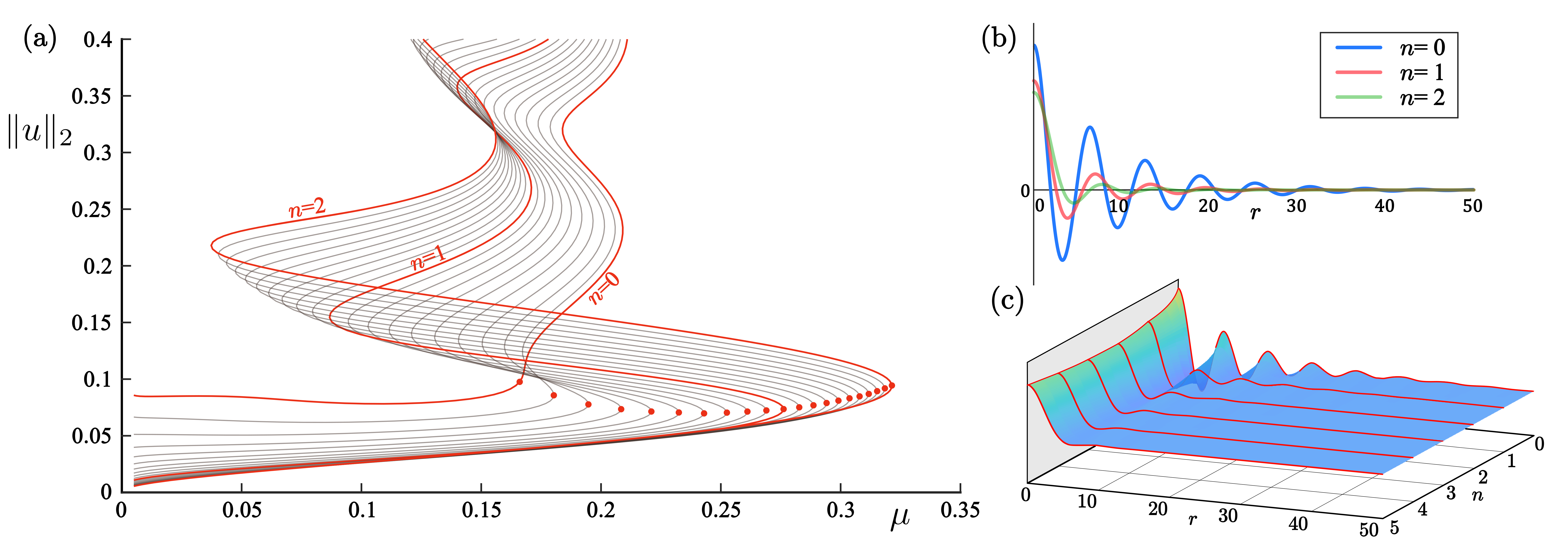
Figure 1: Spot A solutions to (1.3) are computed numerically for $\nu=1.6$ fixed and $\mu,n$ varying. (a) Bifurcation curves of Spot A patterns are plotted with respect to $\mu$ for $0\leq n\leq 2$, where each curve undergoes a fold bifurcation (red spot) and before exhibiting snaking behaviour. Radial profiles of numerical solutions to (1.3) at $\mu=0.05$ are plotted for (b) $n=0,1,2$, and (c) $0<n<5$. The red lines in panel (c) represent integer values of $n$.

Our investigation is also motivated by numerical studies of localised radial patterns. Using numerical continuation codes—such as those available at [5]—one can solve (1.3) to find localised spot A patterns for fixed values of $n$, $\nu$ and track their bifurcation curves as $\mu$ varies; see Figure 1(a). We observe that the bifurcation curves in Figure 1(a) continuously vary as the parameter $n$ changes; each branch grows until it reaches a fold bifurcation and then begins to exhibit snaking behaviour. As $n$ increases, the fold bifurcation becomes more pronounced, and the snaking oscillations become more distorted.

We emphasise here that the parameter $n$ does not just affect the radial profile of each localised pattern, but may also affect the asymptotic scaling of the pattern as it bifurcates from $\mu=0$. Furthermore, while there already exists a prediction for the change in the asymptotic scaling of the spot B solution, the transition between leading order radial functions (i.e. $J_{0}(r)$ when $n=1$ and $\frac{\sin(r)}{r}$ for $n=2$) is less clear, as shown in Figure 1(b-c). The aim of this present work is to extend the approach of [22, 26] to prove the existence of $(n+1)$-dimensional localised radial solutions of (1.2) near a Turing instability in a systematic fashion, such that the entire approach depends continuously on the dimension parameter $n$. We present a novel extension of standard techniques from radial spatial dynamics in order to gain a deeper understanding of the emergence of localised patterns in $(n+1)$ spatial dimensions. As a result of this approach, we not only prove the existence of spot A, spot B and ring patterns in (1.2) for certain values of $n>0$, but we also determine the explicit $n$-dependence of the core profile for each pattern.

The paper is organised as follows. We begin by presenting our main results in § 2, establishing the required hypotheses for (1.2) to undergo a non-degenerate Turing bifurcation and stating our results for the existence of $(n+1)$-dimensional spot and rings patterns. In § 3 we construct the core (§ 3.1) and far-field (§ 3.2-3.4) manifolds that localised radial solutions of (1.2) must intersect. We then employ asymptotic matching to identify intersections between the core and far-field manifolds (§ 3.5), proving our main result for stationary localised radial patterns in systems of the form (1.1) near a Turing bifurcation. Finally, we conclude in § 4 with a discussion of our results and future directions of study.

2 Main Results

In this paper, we assume that $n\in\mathbb{R}$, with $n>0$, and seek localised solutions to (1.2). Throughout we assume $\mathbf{D}(\mu)\in\mathbb{R}^{2\times 2}$ is an invertible matrix for all $\mu$ in some open interval $\mathcal{I}\subset\mathbb{R}$, and $\mathbf{f}\in C^{k}\big{(}\mathbb{R}^{2}\times\mathbb{R},\mathbb{R}^{2}\big{)}$ for $k\geq 3$. We assume that there exists some $\mathbf{u}^{*}\in\mathbb{R}^{2}$ with $\mathbf{f}(\mathbf{u}^{*},\mu)=\mathbf{0}$ for all $\mu\in\mathcal{I}$, such that $\mathbf{u}(r)\equiv\mathbf{u}^{*}$ is a uniform equilibrium for all $\mu\in\mathcal{I}$. Then, we restrict $\mu$ to a neighbourhood of $\mu^{*}$ in $\mathcal{I}$ and apply $\mathbf{D}(\mu)^{-1}$ to (1.2) to normalise the diffusive term $\Delta_{n}\mathbf{u}$.

We proceed by writing $\mathbf{D}(\mu)^{-1}\mathbf{f}(\mathbf{u},\mu)$ as a Taylor expansion about a fixed point $(\mathbf{u},\mu)=(\mathbf{u}^{*},\mu^{*})$, with $\mu^{*}\in\mathcal{I}$, so that (1.2) becomes

$$\mathbf{0}=\Delta_{n}\mathbf{u}-\mathbf{M}_{1}\mathbf{u}-\mu\mathbf{M}_{2}\mathbf{u}-\mathbf{Q}(\mathbf{u},\mathbf{u})-\mathbf{C}(\mathbf{u},\mathbf{u},\mathbf{u})+\mathcal{O}([|\mu|+|\mathbf{u}|]|\mu||\mathbf{u}|+|\mathbf{u}|^{4}).$$ (2.1)

Here we have defined $\mathbf{M}_{1}:=\mathbf{D}(\mu^{*})^{-1}D_{\mathbf{u}}\big{[}\mathbf{f}(\mathbf{u}^{*},\mu^{*})\big{]}$ and introduced $\mathbf{M}_{2}\in\mathbb{R}^{2\times 2}$, $\mathbf{Q}:\mathbb{R}^{2}\times\mathbb{R}^{2}\to\mathbb{R}^{2}$ and $\mathbf{C}:\mathbb{R}^{2}\times\mathbb{R}^{2}\times\mathbb{R}^{2}\to\mathbb{R}^{2}$, where $\mathbf{Q}$ and $\mathbf{C}$ are symmetric bilinear and trilinear maps, respectively. We note that the remainder terms do not affect the subsequent results and so we omit them from our analysis.

With the following hypothesis we make the assumption that (2.1), and hence (1.2), undergoes a nondegenerate Turing instability from the uniform equilibrium $\mathbf{u}=\mathbf{u}^{*}$ at the point $\mu=\mu^{*}$. In what follows $\mathbbm{1}_{m}$ will denote the $m\times m$ identity matrix.

Hypothesis 2.1.

1. (Turing Instability) We assume that $\mathbf{M}_{1}$ satisfies the following condition:

   $$\det\,\big{(}\mathbf{M}_{1}+k_{c}^{2}\mathbbm{1}_{2}\big{)}=0$$

   for some fixed $k_{c}\in\mathbb{R}^{+}$. Furthermore, the eigenvalue $\lambda=-k_{c}^{2}$ of $\mathbf{M}_{1}$ is algebraically double and geometrically simple with generalised eigenvectors $\hat{U}_{0},\hat{U}_{1}\in\mathbb{R}^{2}$, defined so that

   $$\bigg{(}\mathbf{M}_{1}+k_{c}^{2}\mathbbm{1}_{2}\bigg{)}\hat{U}_{0}=\mathbf{0},\qquad\bigg{(}\mathbf{M}_{1}+k_{c}^{2}\mathbbm{1}_{2}\bigg{)}\hat{U}_{1}=k_{c}^{2}\hat{U}_{0},\qquad\langle\hat{U}_{i}^{*},\hat{U}_{j}\rangle_{2}=\delta_{i,j},$$

   for each $i,j\in\{0,1\}$, where $\hat{U}_{0}^{*}$, $\hat{U}_{1}^{*}$ are the respective adjoint vectors for $\hat{U}_{0}$, $\hat{U}_{1}$.

2. (Linear non-degeneracy condition) We assume that $\mathbf{M}_{2}$ satisfies the following condition:

   $$\begin{split}c_{0}:={}&\frac{1}{4}\big{\langle}\hat{U}_{1}^{*},-\mathbf{M}_{2}\hat{U}_{0}\big{\rangle}_{2}\neq 0.\end{split}$$ (2.2)

3. (Quadratic non-degeneracy condition) We assume that $\mathbf{Q}$ satisfies the following condition:

   $$\begin{split}\gamma:=\big{\langle}\hat{U}_{1}^{*},\mathbf{Q}_{0,0}\big{\rangle}_{2}\neq 0,\\ \end{split}$$ (2.3)

   where $\mathbf{Q}_{i,j}:=\mathbf{Q}(\hat{U}_{i},\hat{U}_{j})$.

4. (Cubic non-degeneracy condition) We assume that $\mathbf{Q}$ and $\mathbf{C}$ satisfy the following condition:

   $$\begin{split}c_{3}:=&-\bigg{[}\bigg{(}\frac{5}{6}\big{[}\big{\langle}\hat{U}_{0}^{*},\mathbf{Q}_{0,0}\big{\rangle}_{2}+\big{\langle}\hat{U}_{1}^{*},\mathbf{Q}_{0,1}\big{\rangle}_{2}\big{]}+\frac{19}{18}\big{\langle}\hat{U}_{1}^{*},\mathbf{Q}_{0,0}\big{\rangle}_{2}\bigg{)}\big{\langle}\hat{U}_{1}^{*},\mathbf{Q}_{0,0}\big{\rangle}_{2}+\frac{3}{4}\big{\langle}\hat{U}_{1}^{*},\mathbf{C}_{0,0,0}\big{\rangle}_{2}\bigg{]}\neq 0,\end{split}$$ (2.4)

   where $\mathbf{Q}_{i,j}:=\mathbf{Q}(\hat{U}_{i},\hat{U}_{j})$ and $\mathbf{C}_{i,j,k}:=\mathbf{C}(\hat{U}_{i},\hat{U}_{j},\hat{U}_{k})$.

We briefly remark on the above Hypothesis.

Remark 2.2.

1. Hypothesis 2.1 $(i)$ gives that the linearisation of the right-hand-side of (1.1) about $(\mathbf{u},\mu)=(\mathbf{u}^{*},\mu^{*})$ has a zero eigenvalue, giving way to a Turing bifurcation. We fix $k_{c}=1$ without loss of generality, the wavenumber $k_{c}$ can be reintroduced into our solutions through a coordinate transformation.

2. The constant $c_{0}$ in Hypothesis 2.1 $(ii)$ determines the direction of bifurcation for localised radial patterns; localised patterns emerge for $\mu>0$ when $c_{0}>0$, and for $\mu<0$ when $c_{0}<0$. We assume that $c_{0}>0$, since we can otherwise define $\tilde{\mu}:=-\mu$ and $\tilde{c}_{0}:=-c_{0}>0$ so that localised patterns emerge for $\tilde{\mu}>0$.

3. The non-degeneracy conditions in Hypothesis 2.1 $(iii)$, $(iv)$ are sufficient, but not necessary, conditions for localised patterns to emerge. Spot A patterns require $\gamma\neq 0$ but not $c_{3}\neq 0$, ring patterns require $c_{3}\neq 0$ but not $\gamma\neq 0$, while spot B patterns require both $\gamma\neq 0$ and $c_{3}\neq 0$.

Remark 2.3.

We note that the quadratic-cubic Swift–Hohenberg equation (1.3) is contained within the framework of (2.1), where $\mathbf{u}=(u,(1+\Delta_{n})u)^{T}$, $\hat{U}_{0}=(1,0)^{T}$, $\hat{U}_{1}=(0,1)^{T}$, and

$$\mathbf{Q}(\mathbf{u},\mathbf{u})=\begin{pmatrix}0\\ \nu u^{2}\end{pmatrix},\qquad\mathbf{C}(\mathbf{u},\mathbf{u},\mathbf{u})=\begin{pmatrix}0\\ -u^{3}\end{pmatrix},\qquad\mathbf{M}_{1}=\begin{pmatrix}-1&1\\ 0&-1\end{pmatrix},\qquad\mathbf{M}_{2}=\begin{pmatrix}0&0\\ -1&0\end{pmatrix}.$$

Then, $c_{0}=\frac{1}{4}$, $\gamma=\nu$ and $c_{3}=\frac{3}{4}-\frac{19\nu^{2}}{18}$.

Following the approach of [22, 26], we employ tools from the radial spatial dynamics theory of Scheel [31] to prove the existence of localised radial solutions to (2.1). To do this, we construct two local invariant manifolds—the ‘core manifold’ $\mathcal{W}^{cu}_{-}(\mu)$ and the ‘far-field manifold’ $\mathcal{W}^{s}_{+}(\mu)$—over local intervals $r\in[0,r_{0}]$ and $r\in[r_{0},\infty)$, respectively, where the point $r_{0}>0$ is chosen to be large. The core manifold consists of all small-amplitude solutions of (2.1) that remain bounded as $r\to 0^{+}$, while the far-field manifold consists of all small-amplitude solutions of (2.1) that decay exponentially fast as $r\to\infty$. After constructing each manifold, we use asymptotic matching to find trajectories that lie on the intersection of both manifolds. These trajectories consist of solutions of (2.1) that are bounded for all $r\in[0,\infty)$ and decay exponentially fast as $r\to\infty$, thus defining localised radial solutions to (2.1).

To make use of the radial structure of (1.2), we introduce the following objects that will be useful when considering $(n+1)$-dimensional radial functions.

Definition 2.4.

We define the $k$-index Bessel operator $\mathcal{D}_{k}$ to be the nonautonomous differential operator

$$\mathcal{D}_{k}:u(r)\mapsto r^{-k}\,\partial_{r}\,(r^{k}u(r))=\left(\partial_{r}+\tfrac{k}{r}\right)u(r)$$ (2.5)

for any $k\in\mathbb{R}$ (see [14]) and we note that the following identities

$$\mathcal{D}_{i}\mathcal{D}_{j}=\mathcal{D}_{j+1}\mathcal{D}_{i-1},\qquad\qquad\mathcal{D}_{i}(r^{{j}}u(r))=r^{j}\mathcal{D}_{i+j}u(r),\qquad\qquad\Delta_{n}=\mathcal{D}_{n}\mathcal{D}_{0},$$ (2.6)

hold for all $i,j\in\mathbb{R}$, where $\Delta_{n}$ is the $(n+1)$-dimensional Laplace operator.

Additionally, we define the $(n+1)$-dimensional Bessel functions of the first and second kind to be

$$J^{(n)}_{\ell}(r):=2^{(\frac{n-1}{2})}\Gamma\left(\frac{n+1}{2}\right)r^{-(\frac{n-1}{2})}J_{\ell+\frac{n-1}{2}}(r),\qquad Y^{(n)}_{\ell}(r):=2^{(\frac{n-1}{2})}\Gamma\left(\frac{n+1}{2}\right)r^{-(\frac{n-1}{2})}Y_{\ell+\frac{n-1}{2}}(r),$$ (2.7)

respectively, where $J_{\nu}(r)$, $Y_{\nu}(r)$ are the respective $\nu$-th order Bessel functions of the first and second kind.

The Bessel operators $\mathcal{D}_{k}$, with $k\in\mathbb{Z}$, were recently introduced in [14] as the natural differential operators for planar functions of the form $\mathrm{e}^{\mathrm{i}k\theta}f_{k}(r)$. While the theory presented in [14] is restricted to functions of two-dimensional polar (or three-dimensional cylindrical) coordinates, the Bessel operators are also helpful in our study of radial functions in higher spatial dimensions.

The $(n+1)$-dimensional Bessel functions (also known as hyperspherical Bessel functions) $J_{\ell}^{(n)}(r),Y_{\ell}^{(n)}(r)$ were previously introduced in [39], and have recently been employed in the study of pattern formation in nonlocal transport models for cell interaction [19]; see also § 10 in [4] for more information. We briefly note some important properties of these functions.

Remark 2.5.

The $(n+1)$-dimensional Bessel functions $Z^{(n)}_{\ell}(r)\in\{J^{(n)}_{\ell}(r),Y^{(n)}_{\ell}(r)\}$ are defined so that

1. $J^{(n)}_{0}(0)=1$ for all $n>0$,

2. $\mathcal{D}_{n-1+\ell}\,Z_{\ell}^{(n)}(r)=Z_{\ell-1}^{(n)}$, $\mathcal{D}_{-\ell}\,Z_{\ell}^{(n)}(r)=-Z_{\ell+1}^{(n)}$ for all $n,\ell\in\mathbb{R}$,

3. $J_{\ell}^{(0)}(r)=\cos(r)$, $Y_{\ell}^{(0)}(r)=\sin(r)$, $J_{\ell}^{(1)}(r)=J_{\ell}(r)$, $Y_{\ell}^{(1)}(r)=Y_{\ell}(r)$, and $J_{\ell}^{(2)}(r)=j_{\ell}(r)$, $Y_{\ell}^{(2)}(r)=y_{\ell}(r)$, where $j_{\ell}(r),y_{\ell}(r)$ are $\ell$-th order spherical Bessel functions of the first and second kind, respectively.

Furthermore, the $(n+1)$-dimensional Bessel functions satisfy the following generalised form of Bessel’s equation

$$(\mathcal{D}_{n+\ell}\mathcal{D}_{-\ell}+1)r^{\alpha}Z_{\ell+\alpha}^{(n)}(r)=2\alpha\,r^{\alpha-1}\,Z_{\ell+\alpha-1}^{(n)}(r),$$

for any $n,\ell,\alpha\in\mathbb{R}$.

The functions $\{J_{0}^{(n)}(r),rJ_{1}^{(n)}(r),Y_{0}^{(n)}(r),rY_{1}^{(n)}(r)\}$ thus form a linearly independent set of solutions to the equation $(\Delta_{n}+1)^{2}u=0$, which corresponds to the linearisation of (2.1) at $\mu=0$. In Lemma 3.1 we use a variation-of-constants formula with this set of linear solutions in order to construct core manifold $\mathcal{W}^{cu}_{-}(\mu)$ on a bounded interval $r\in[0,r_{0}]$.

In order to construct the far-field manifold $\mathcal{W}^{s}_{+}(\mu)$, we introduce complex coordinates $A,B$ so that the system (2.1) is transformed into the radial normal form for an $(n+1)$-dimensional Hamiltonian–Hopf bifurcation. Upon introducing the far-field radial coordinate $s:=\mu^{\frac{1}{2}}r$, exponentially decaying solutions are then found to be $\mathcal{O}(\mu^{\frac{1}{2}})$-perturbations of the non-autonomous cubic Ginzburg–Landau equation

$$\left(\frac{\mathrm{d}}{\mathrm{d}s}+\frac{n}{2s}\right)^{2}A=c_{0}A+c_{3}|A|^{2}A,\qquad A\in\mathbb{C},\qquad s\in[0,\infty),$$ (2.8)

where $c_{0}$ and $c_{3}$ are defined in (2.2) and (2.4), respectively. Localised ring and spot B solutions require the existence of a nontrivial forward-bounded localised solution to (2.8), and so the authors of [22, 26] employed the following hypothesis.

Hypothesis 2.6.

Fix $n>0$. The equation

$$\left(\frac{\mathrm{d}}{\mathrm{d}s}+\frac{n}{2s}\right)^{2}A=A-A^{3},\qquad A\in\mathbb{R},\qquad s\in[0,\infty)$$ (2.9)

has a forward-bounded nontrivial localised solution $A(s)=q(s)$. In addition, the linearisation of (2.9) about $q(s)$ possesses no nontrivial solutions that are forward-bounded on $[0,\infty)$.

It is straightforward to prove this hypothesis when $n=2$ as the differential operator becomes the three-dimensional radial Laplacian and one can employ theory from the vast literature on elliptic PDEs (see Lemma 4.3 in [26] and the references therein). However, it is not clear that this result holds for any other values of $n>0$, this hypothesis was eventually proven in the case when $n=1$ by van den Berg et al. in [35] via a computer-assisted proof.

In this work, we present a simplified proof of Hypothesis 2.6 for any choice of $n>0$. Our proof relies on the following proposition which can be proven using standard elliptic PDE theory.

Proposition 2.7.

The equation

$$\Delta u=u-|\mathbf{x}|^{2-n}u^{3},\qquad u\in\mathbb{R},\qquad\mathbf{x}\in\mathbb{R}^{3}$$ (2.10)

has a positive radial ground state solution $u(\mathbf{x})=Q(|\mathbf{x}|)$ for any $n>0$. In addition, the linearisation of (2.10) about $Q(|\mathbf{x}|)$

$$\mathcal{L}\,v:=\left(-\Delta+1-3|\mathbf{x}|^{2-n}Q(|\mathbf{x}|)^{2}\right)v=0,\qquad v\in\mathbb{R},\qquad\mathbf{x}\in\mathbb{R}^{3}$$ (2.11)

possesses no nontrivial radial solutions that are bounded uniformly on $[0,\infty)$.

Proof.

Existence of a radial positive ground state follows from standard variational methods for $n>2$ (see for example [20, 21, 33]), and follows directly from [12] for $0<n\leq 2$. The nonexistence of bounded solutions to (2.11) follows from the proof of Lemma 2.1 in [10], where we use the fact that the two quantities $Q(r)$, $Q_{1}(r):=r\mathcal{D}_{\frac{4-n}{2}}Q(r)$ satisfy $\mathcal{L}Q(|\mathbf{x}|)=-2|\mathbf{x}|^{2-n}Q(|\mathbf{x}|)^{3}$ and $\mathcal{L}Q_{1}(|\mathbf{x}|)=-2Q(|\mathbf{x}|)$. ∎

In Lemma 3.4 we show that Proposition 2.7 implies Hypothesis 2.6 and thus guarantees the existence of localised ring and spot B solutions to (2.1) for $0<n<4$. We present our key result in the following theorem.

Theorem 2.8.

Fix $n>0$ and assume Hypotheses 2.1 (i-ii) hold. Then, there exist constants $\mu_{0},r_{0},r_{1}>0$ such that the system (2.1) has radially localised solutions for each $\mu\in(0,\mu_{0})$. Each respective solution decays at a rate $\mathcal{O}(r^{-\frac{n}{2}}\mathrm{e}^{-\sqrt{c_{0}\mu}\,r})$ as $r\to\infty$ and satisfies the following equations uniformly on bounded intervals $[0,r_{0}]$ as $\mu\to 0^{+}$.

1. (Spot A) If Hypothesis 2.1 (iii) holds, then we obtain

   $$\begin{split}\mathbf{u}_{A}(r)={}&(c_{0}\mu)^{\frac{1}{2}}\left(\frac{\sqrt{\pi}}{\nu_{n}\gamma}\right)\frac{1}{2^{\frac{n}{2}}\Gamma(\frac{n+1}{2})}J_{0}^{(n)}(r)\hat{U}_{0}+\mathcal{O}(\mu),\\ \end{split}$$ (2.12)

2. (Rings) If $n<4$ and Hypothesis 2.1 (iv) holds with $c_{3}<0$, then we obtain

   $$\begin{split}\mathbf{u}_{R}(r)={}&\pm(c_{0}\mu)^{\frac{4-n}{4}}\left(\frac{2\sqrt{\pi}q_{n}}{\sqrt{|c_{3}|}}\right)\frac{1}{2^{\frac{n}{2}}\Gamma(\frac{n+1}{2})}\left[rJ_{1}^{(n)}(r)\hat{U}_{0}+2J_{0}^{(n)}(r)\hat{U}_{1}\right]+\mathcal{O}(\mu^{\frac{6-n}{4}}+\mu^{\frac{4-n}{2}}),\\ \end{split}$$ (2.13)

3. (Spot B) If $n<4$ and Hypotheses 2.1 (iii-iv) hold with $c_{3}<0$, then we obtain

   $$\begin{split}\mathbf{u}_{B}(r)={}&-\mathrm{sgn}(\gamma)(c_{0}\mu)^{\frac{4-n}{8}}\left(\frac{\pi q_{n}}{\nu_{n}|\gamma|\sqrt{|c_{3}|}}\right)^{\frac{1}{2}}\frac{1}{2^{\frac{n-1}{2}}\Gamma(\frac{n+1}{2})}J_{0}^{(n)}(r)\hat{U}_{0}+\mathcal{O}(\mu^{\frac{8-n}{8}}+\mu^{\frac{4-n}{4}}),\\ \end{split}$$ (2.14)

Here, $\gamma,c_{0},c_{3}$ are defined in Hypothesis 2.1, $q_{n}:=\displaystyle\lim_{s\to 0}Q(s)$, where $Q(|\mathbf{x}|)$ is the positive radial ground state solution of (2.10),

$$\nu_{n}:=\left(\frac{3}{8}\right)^{\frac{n}{2}}\frac{\pi}{3\Gamma(\frac{n}{2})},$$ (2.15)

and $J^{(n)}_{\ell}(r)$ is the $(n+1)$-dimensional $\ell^{\mathrm{th}}$ order Bessel function of the first kind defined in (2.7).

Furthermore, for $c_{3}>0$, spot A solutions given by (2.12) undergo a fold bifurcation along the curve

$$\gamma=\pm(c_{0}\mu)^{\frac{1}{4}}\left(\frac{(\mu^{-\frac{1}{2}}r_{1})^{n-1}-r_{0}^{n-1}}{(n-1)(\mu^{-\frac{1}{2}}r_{1})^{n-1}\,r_{0}^{n-1}}\right)^{\frac{1}{2}}\,\left(\frac{|c_{3}|^{\frac{1}{2}}}{\nu_{n}}\right)(1+\mathrm{o}(1))$$ (2.16)

as $\mu\to 0^{+}$.

For planar patterns $\nu_{n}=\frac{1}{2}\sqrt{\frac{\pi}{6}}$ and for spherical patterns $\nu_{n}=\frac{\pi}{8}$, which are both in agreement with [22, 26]. While we are unable to derive a closed form expression for $q_{n}$ in the same way as for $\nu_{n}$, we can numerically compute its value for different choices of $n$. We present plots of both $\nu_{n}$ and $q_{n}$ in Figure 2.

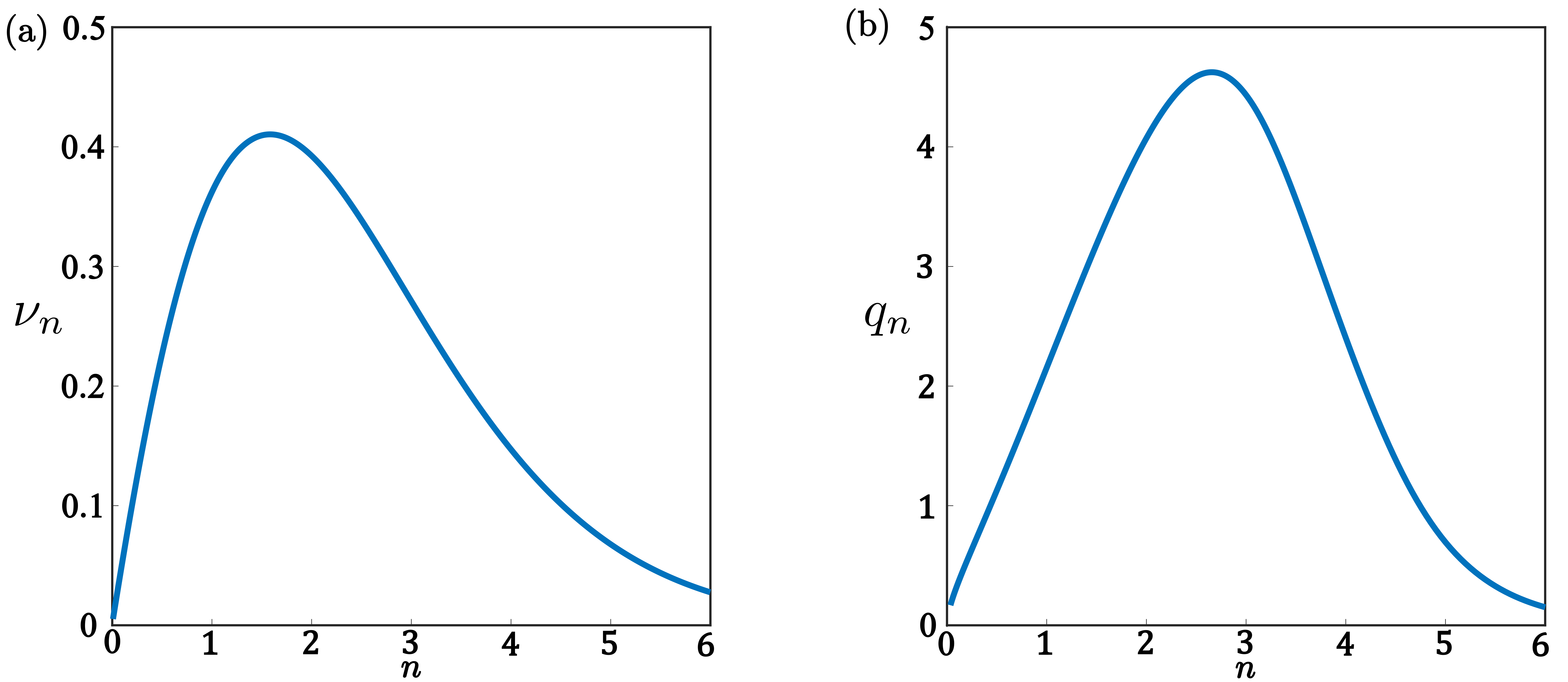
Figure 2: A plot of the values of (a) $\nu_{n}$ and (b) $q_{n}$ for $0<n<6$.

3 Proof of Theorem 2.8

We begin by expressing (2.1) as the following first-order system,

$$\frac{\textnormal{d}}{\textnormal{d}r}\mathbf{U}=\mathcal{A}(r)\mathbf{U}+\mathbf{F}(\mathbf{U},\mu),$$ (3.1)

where $\mathbf{U}:=(\mathbf{u},\mathcal{D}_{0}\mathbf{u})^{T}$, with

$$\mathcal{A}(r) =\begin{pmatrix}\mathbb{O}_{2}&\mathbbm{1}_{2}\\ \mathbf{M}_{1}&-\frac{n}{r}\mathbbm{1}_{2}\end{pmatrix},\quad\mathbf{F}(\mathbf{U};\mu)=\begin{pmatrix}\mathbf{0}\\ \displaystyle\mu\mathbf{M}_{2}\mathbf{u}+\mathbf{Q}(\mathbf{u},\mathbf{u})+\mathbf{C}(\mathbf{u},\mathbf{u},\mathbf{u})\end{pmatrix},$$

where we recall that $\mathbb{O}_{2}$ and $\mathbbm{1}_{2}$ denote the $2\times 2$ zero and identity matrices, respectively.

3.1 The Core Manifold

We construct the core manifold $\mathcal{W}_{-}^{cu}(\mu)$, for $0<\mu\ll 1$, which contains all small-amplitude solutions to (2.1) that remain bounded as $r\to 0$. This is a local invariant manifold, and so we determine it on a bounded interval $r\in[0,r_{0}]$, for some fixed $r_{0}>0$. We first note that, at the bifurcation point $\mu=0$, the linearisation of (3.1) about $\mathbf{U}=\mathbf{0}$, given by

$$\frac{\textnormal{d}}{\textnormal{d}r}\mathbf{V}=\mathcal{A}(r)\mathbf{V},$$ (3.2)

has solutions of the form

$$\mathbf{V}(r)=\sum_{j=1}^{4}d_{j}\mathbf{V}_{j}(r),$$ (3.3)

with

$$\begin{split}\mathbf{V}_{1}(r)&=\frac{\sqrt{\pi}}{2^{\frac{n}{2}}\Gamma(\frac{n+1}{2})}\begin{pmatrix}J^{(n)}_{0}(r)\hat{U}_{0}\\ -J^{(n)}_{1}(r)\hat{U}_{0}\end{pmatrix},\\ \mathbf{V}_{2}(r)&=\frac{\sqrt{\pi}}{2^{\frac{n}{2}}\Gamma(\frac{n+1}{2})}\begin{pmatrix}rJ^{(n)}_{1}(r)\hat{U}_{0}+2J^{(n)}_{0}(r)\hat{U}_{1}\\ [rJ^{(n)}_{0}(r)-(n-1)J_{1}^{(n)}(r)]\hat{U}_{0}-2J^{(n)}_{1}(r)\hat{U}_{1}\end{pmatrix},\\ \mathbf{V}_{3}(r)&=\frac{\sqrt{\pi}}{2^{\frac{n}{2}}\Gamma(\frac{n+1}{2})}\begin{pmatrix}Y^{(n)}_{0}(r)\hat{U}_{0}\\ -Y^{(n)}_{1}(r)\hat{U}_{0}\end{pmatrix},\\ \mathbf{V}_{4}(r)&=\frac{\sqrt{\pi}}{2^{\frac{n}{2}}\Gamma(\frac{n+1}{2})}\begin{pmatrix}rY^{(n)}_{1}(r)\hat{U}_{0}+2Y^{(n)}_{0}(r)\hat{U}_{1}\\ [rY^{(n)}_{0}(r)-(n-1)Y_{1}^{(n)}(r)]\hat{U}_{0}-2Y^{(n)}_{1}(r)\hat{U}_{1}\end{pmatrix}.\end{split}$$ (3.4)

To see how we arrive at the above solutions for $\mathbf{u}$, we recall that the system $\frac{\textnormal{d}}{\textnormal{d}r}\mathbf{V}=\mathcal{A}(r)\mathbf{V}$ is equivalent to

$$\left(\mathcal{D}_{n}\mathcal{D}_{0}-\mathbf{M}_{1}\right)\mathbf{u}=\mathbf{0}$$ (3.5)

where $\mathbf{V}=(\mathbf{u},\mathcal{D}_{0}\mathbf{u})^{T}$. Decomposing $\mathbf{u}=u_{1}\hat{U}_{0}+u_{2}\hat{U}_{1}$, we then obtain

$$\left(\mathcal{D}_{n}\mathcal{D}_{0}+1\right)u_{1}=u_{2},\qquad\qquad\left(\mathcal{D}_{n}\mathcal{D}_{0}+1\right)u_{2}=0,$$ (3.6)

which has solutions $u_{2}=2c_{2}J_{0}^{(n)}(r)+2c_{4}Y_{n}^{(n)}(r)$ and $u_{1}=c_{1}J_{0}^{(n)}(r)+c_{2}rJ_{1}^{(n)}(r)+c_{3}Y_{n}^{(n)}(r)+c_{4}rY_{1}^{(n)}(r)$.

We now present a standard result regarding the existence and parametrisation of $\mathcal{W}^{cu}_{-}(\mu)$ on the interval $[0,r_{0}]$, for $0<\mu\ll 1$. In what follows we will use the Landau symbol $\mathcal{O}_{r_{0}}(\cdot)$ with the meaning of the standard Landau symbol $\mathcal{O}(\cdot)$ except that the bounding constants may depend on the value of $r_{0}$.

Function	as $r\to 0$	as $r\to\infty$
$J^{(n)}_{\ell}(r)$	$\mathcal{O}\left(r^{\ell}\right)$	$\frac{2^{\frac{n}{2}}\Gamma\left(\frac{n+1}{2}\right)}{\sqrt{\pi}}r^{-\frac{n}{2}}\cos\left(r-\frac{n\pi}{4}-\frac{\ell\pi}{2}\right)+\mathcal{O}\left(r^{-(\frac{n+2}{2})}\right)$
$Y^{(n)}_{\ell}(r)$	$\mathcal{O}\left(r^{\ell}\left(\cot(\nu\pi)-\frac{2^{2\nu}\Gamma(\nu)\Gamma(\nu+1)}{r^{2\nu}\pi}\right)_{\nu=\ell+\frac{n-1}{2}}\right)$	$\frac{2^{\frac{n}{2}}\Gamma\left(\frac{n+1}{2}\right)}{\sqrt{\pi}}r^{-\frac{n}{2}}\sin\left(r-\frac{n\pi}{4}-\frac{\ell\pi}{2}\right)+\mathcal{O}\left(r^{-(\frac{n+2}{2})}\right)$

Table 1: Orders and expansions for $(n+1)$-dimensional $\ell$’th-order Bessel functions of the first and second kind as $r\to 0$ and $r\to\infty$, respectively, where $n\in\mathbb{R}$, $n\geq 0$; see [1, (9.1.10),(9.1.11), and §9.2].

Lemma 3.1.

For each fixed $r_{0}>0$, there are constants $\delta_{1},\delta_{2}>0$ such that the set $\mathcal{W}^{cu}_{-}(\mu)$ of solutions $\mathbf{U}(r)$ of (3.1) for which $\sup_{0\leq r\leq r_{0}}\|\mathbf{U}(r)\|<\delta_{1}$ is, for $|\mu|<\delta_{1}$, a smooth $2$ dimensional manifold. Furthermore, each $\mathbf{U}(r_{0})\in\mathcal{W}^{cu}_{-}(\mu)$ with $|\mathcal{P}^{cu}_{-}(r_{0})\mathbf{U}(r_{0})|<\delta_{2}$ can be written uniquely as

$$\begin{split}\mathbf{U}(r_{0})&=d_{1}\mathbf{V}_{1}(r_{0})+d_{2}\mathbf{V}_{2}(r_{0})+\mathbf{V}_{3}(r_{0})\mathcal{O}_{r_{0}}(|\mu||\mathbf{d}|+|\mathbf{d}|^{2})\\ &\qquad\qquad+\mathbf{V}_{4}(r_{0})\left[\left(\nu_{n}+\mathcal{O}\left(r_{0}^{-\frac{n}{2}}\right)\right)\gamma\,d_{1}^{2}+\mathcal{O}_{r_{0}}(|\mu||\mathbf{d}|+|d_{2}|^{2}+|d_{1}|^{3})\right],\end{split}$$ (3.7)

where $\gamma$ is defined in (2.3), $\nu_{n}$ is defined in (2.15) for all $n>0$, $\mathbf{d}:=\left(d_{1},d_{2}\right)\in\mathbb{R}^{2}$ with $|\mathbf{d}|<\delta_{2}$, and the right-hand side of (3.7) depends smoothly on $(\mathbf{d},\mu)$.

Proof.

This statement is proven in a similar way to several previously proven lemmata; see, for example, [22, Lemma 1] or [16, Lemma 4.1]. To do this, we first note that the linear adjoint problem $\frac{\textnormal{d}}{\textnormal{d}r}\mathbf{W}=-\mathcal{A}^{T}(r)\mathbf{W}$ has independent solutions of the form

$$\begin{split}\mathbf{W}_{1}&=\frac{\sqrt{\frac{\pi}{2}}}{2^{(\frac{n+1}{2})}\Gamma(\frac{n+1}{2})}\begin{pmatrix}r^{n}\left[rY^{(n)}_{0}(r)\hat{U}_{1}^{*}-2Y^{(n)}_{1}(r)\hat{U}_{0}^{*}\right]\\ -r^{n}\left[[rY^{(n)}_{1}(r)-(n-1)Y_{n}^{(n)}(r)]\hat{U}_{1}^{*}+2Y^{(n)}_{0}(r)\hat{U}_{0}^{*}\right]\end{pmatrix},\\ \mathbf{W}_{2}&=\frac{\sqrt{\frac{\pi}{2}}}{2^{(\frac{n+1}{2})}\Gamma(\frac{n+1}{2})}\begin{pmatrix}-r^{n}Y^{(n)}_{1}(r)\hat{U}_{1}^{*}\\ -r^{n}Y^{(n)}_{0}(r)\hat{U}_{1}^{*}\end{pmatrix},\\ \mathbf{W}_{3}&=\frac{\sqrt{\frac{\pi}{2}}}{2^{(\frac{n+1}{2})}\Gamma(\frac{n+1}{2})}\begin{pmatrix}-r^{n}\left[rJ^{(n)}_{0}(r)\hat{U}_{1}^{*}-2J^{(n)}_{1}(r)\hat{U}_{0}^{*}\right]\\ r^{n}\left[[rJ^{(n)}_{1}(r)-(n-1)J_{0}^{(n)}(r)]\hat{U}_{1}^{*}+2J^{(n)}_{0}(r)\hat{U}_{0}^{*}\right]\end{pmatrix},\\ \mathbf{W}_{4}&=\frac{\sqrt{\frac{\pi}{2}}}{2^{(\frac{n+1}{2})}\Gamma(\frac{n+1}{2})}\begin{pmatrix}r^{n}J^{(n)}_{1}(r)\hat{U}_{1}^{*}\\ r^{n}J^{(n)}_{0}(r)\hat{U}_{1}^{*}\end{pmatrix}.\end{split}$$ (3.8)

such that the relation

$$\langle\mathbf{W}_{i}(r),\mathbf{V}_{j}(r)\rangle_{4}=\delta_{i,j}$$ (3.9)

holds for all $r\in\mathbb{R}$, $i,j\in\{1,2,3,4\}$. For a given $\mathbf{d}=(d_{1},d_{2})\in\mathbb{R}^{2(N+1)}$, we consider the fixed-point equation

$$\begin{split}\mathbf{U}(r)&=\sum_{j=1}^{2}d_{j}\mathbf{V}_{j}(r)+\sum_{j=1}^{2}\mathbf{V}_{j}(r)\int_{r_{0}}^{r}\langle\mathbf{W}_{j}(s),\mathbf{F}(\mathbf{U}[s];\mu)\rangle_{4}\,\textnormal{d}s+\sum_{j=3}^{4}\mathbf{V}_{j}(r)\int_{0}^{r}\langle\mathbf{W}_{j}(s),\mathbf{F}(\mathbf{U}[s];\mu)\rangle_{4}\,\textnormal{d}s,\end{split}$$ (3.10)

on $C([0,r_{0}],\mathbb{R}^{4})$ and prove that (3.10) defines a contraction for sufficiently small $\mathbf{d}$ and $\mu$. Evaluating (3.10) at $r=r_{0}$, we arrive at

$$\mathbf{U}(r_{0})=\sum_{j=1}^{2}d_{j}\mathbf{V}_{j}(r_{0})+\sum_{j=3}^{4}\mathbf{V}_{j}(r_{0})\int_{0}^{r_{0}}\langle\mathbf{W}_{j}(s),\mathbf{F}(\mathbf{U}[s];\mu)\rangle_{4}\,\textnormal{d}s.$$ (3.11)

Then, we introduce

$$c_{j}\left(d_{1},d_{2};\mu\right):=\int_{0}^{r_{0}}\langle\mathbf{W}_{j}(s),\mathbf{F}(\mathbf{U}[s];\mu)\rangle_{4}\,\textnormal{d}s,$$ (3.12)

for $j=3,4$ so that we can write our small-amplitude core solution as

$$\mathbf{U}(r_{0})=d_{1}\mathbf{V}_{1}(r_{0})+d_{2}\mathbf{V}_{2}(r_{0})+c_{3}\left(d_{1},d_{2};\mu\right)\mathbf{V}_{3}(r_{0})+c_{4}\left(d_{1},d_{2};\mu\right)\mathbf{V}_{4}(r_{0}).$$ (3.13)

In order to arrive at (3.7), we apply a Taylor expansion to (3.12) about $|d_{1}|=|d_{2}|=\mu=0$ and find

$$\begin{split}c_{3}\left(d_{1},d_{2};\mu\right)&=\mathcal{O}_{r_{0}}\left(|\mu||\mathbf{d}|+|\mathbf{d}|^{2}\right),\\ c_{4}\left(d_{1},d_{2};\mu\right)&=\left[\nu_{n}+\mathcal{O}\left(r_{0}^{-\frac{n}{2}}\right)\right]\gamma\,d_{1}^{2}+\mathcal{O}_{r_{0}}\left(|\mu||\mathbf{d}|+|d_{2}|^{2}+|d_{1}|^{3}\right),\\ \end{split}$$ (3.14)

where $\gamma=\langle\hat{U}_{1}^{*},\mathbf{Q}(\hat{U}_{0},\hat{U}_{0})\rangle_{2}$ and

$$\nu_{n}:=\frac{1}{2}\left(\frac{\sqrt{\frac{\pi}{2}}}{2^{(\frac{n-1}{2})}\Gamma(\frac{n+1}{2})}\right)^{3}\int_{0}^{\infty}s^{n}(J_{0}^{(n)}(s))^{3}\,\textnormal{d}s.$$ (3.15)

Here, we have used the fact that

$$\int_{r_{0}}^{\infty}s^{n}(J_{0}^{(n)}(s))^{3}\,\textnormal{d}s=\mathcal{O}\left(r_{0}^{-\frac{n}{2}}\right)$$

for $n>0$ and $r_{0}\gg 1$ in order to determine the order of the remainder terms. We compute the explicit value of $\nu_{n}$, obtaining

$$\begin{split}\nu_{n}={}&\frac{1}{2}\left(\frac{\sqrt{\frac{\pi}{2}}}{2^{(\frac{n-1}{2})}\Gamma(\frac{n+1}{2})}\right)^{3}\int_{0}^{\infty}s^{n}(J_{0}^{(n)}(s))^{3}\,\textnormal{d}s,\\ ={}&\frac{\pi\sqrt{\pi}}{4\sqrt{2}}\int_{0}^{\infty}s^{1-(\frac{n-1}{2})}(J_{\frac{n-1}{2}}(s))^{3}\,\textnormal{d}s,\\ ={}&\left(\frac{3}{8}\right)^{\frac{n}{2}}\frac{\pi}{3\Gamma(\frac{n}{2})}.\\ \end{split}$$ (3.16)

This completes the proof. ∎

We conclude this section by noting the following. For sufficiently large $r_{0}$, we can use Table 1 to write (3.7) in terms of its elements $\mathbf{u}(r_{0}),\mathbf{v}(r_{0})\in\mathbb{R}^{2}$, where

$$\begin{split}\mathbf{u}(r_{0})&=r_{0}^{-\frac{n}{2}}\left[d_{2}r_{0}\left(1+\mathcal{O}(r_{0}^{-1})\right)\sin\left(y_{n}\right)+d_{1}\left(1+\mathcal{O}(r_{0}^{-1})\right)\cos\left(y_{n}\right)+\mathcal{O}_{r_{0}}(|\mu||\mathbf{d}|+|\mathbf{d}|^{2})\right]\hat{U}_{0}\\ &\qquad+2r_{0}^{-\frac{n}{2}}\Big{[}\gamma\,d_{1}^{2}\left(\nu_{n}+\mathcal{O}(r_{0}^{-\frac{n}{2}}+r_{0}^{-1})\right)\sin\left(y_{n}\right)+d_{2}\left(1+\mathcal{O}(r_{0}^{-1})\right)\cos\left(y_{n}\right)\\ &\hskip 233.3125pt+\mathcal{O}_{r_{0}}(|\mu||\mathbf{d}|+|d_{2}|^{2}+|d_{1}|^{3})\Big{]}\hat{U}_{1}\\ \mathbf{v}(r_{0})&=r_{0}^{-\frac{n}{2}}\left[d_{2}r_{0}\left(1+\mathcal{O}(r_{0}^{-1})\right)\cos\left(y_{n}\right)-d_{1}\left(1+\mathcal{O}(r_{0}^{-1})\right)\sin\left(y_{n}\right)+\mathcal{O}_{r_{0}}(|\mu||\mathbf{d}|+|\mathbf{d}|^{2})\right]\hat{U}_{0}\\ &\qquad+2r_{0}^{-\frac{n}{2}}\Big{[}\gamma\,d_{1}^{2}\left(\nu_{n}+\mathcal{O}(r_{0}^{-\frac{n}{2}}+r_{0}^{-1})\right)\cos\left(y_{n}\right)-d_{2}\left(1+\mathcal{O}(r_{0}^{-1})\right)\sin\left(y_{n}\right)\\ &\hskip 233.3125pt+\mathcal{O}_{r_{0}}(|\mu||\mathbf{d}|+|d_{2}|^{2}+|d_{1}|^{3})\Big{]}\hat{U}_{1}\\ \end{split}$$ (3.17)

Here we have written $y_{n}:=r_{0}-\frac{n\pi}{4}$, while the $\mathcal{O}_{r_{0}}(\cdot)$ remainders capture the higher order terms when $|\mathbf{d}|$ and $|\mu|$ are taken to be small.

3.2 The Far-Field Manifold

We now turn to parametrising the far-field manifold $\mathcal{W}_{+}^{s}(\mu)$, consisting of all small-amplitude solutions to (2.1) that decay to zero exponentially fast as $r\to\infty$. We introduce the variable $\sigma(r)\geq 0$ to take the place of the $\frac{1}{r}$ terms in (3.1). The result is the extended autonomous system

$$\begin{split}\frac{\textnormal{d}}{\textnormal{d}r}\mathbf{U}&=\mathcal{A}(\infty)\mathbf{U}+\widetilde{\mathbf{F}}(\mathbf{U};\mu,\sigma),\\ \frac{\textnormal{d}}{\textnormal{d}r}\sigma&=-\sigma^{2},\end{split}$$ (3.18)

with the property that $\sigma(r)=r^{-1}$ is an invariant manifold of (3.18), and by definition this invariant manifold recovers the non-autonomous system (3.1). To construct the far-field manifold $\mathcal{W}^{s}_{+}(\mu)$ we find the set of all small-amplitude solutions $(\mathbf{U},\sigma)(r)$ to (3.18) such that $\mathbf{U}(r)$ decays exponentially as $r\to\infty$. Then, evaluating at $\sigma(r_{0})=r_{0}^{-1}$, we restrict our solutions to the invariant subspace $\sigma(r)=r^{-1}$, such that $\mathbf{U}(r)$ is an exponentially decaying solution of (3.1).

Before attempting to find exponentially decaying solutions to (3.18), we first transform the system into the normal form for an $n$-dimensional Hamiltonian–Hopf bifurcation. We define complex amplitudes $\widetilde{A},\widetilde{B}$, which satisfy the following relations

$$\mathbf{u} =(\widetilde{A}+\overline{\widetilde{A}})\hat{U}_{0}+2\textnormal{i}(\widetilde{B}-\overline{\widetilde{B}})\hat{U}_{1}, \qquad\mathbf{v} =\big{[}\textnormal{i}(\widetilde{A}-\overline{\widetilde{A}})+(\widetilde{B}+\overline{\widetilde{B}})\big{]}\hat{U}_{0}-2(\widetilde{B}+\overline{\widetilde{B}})\hat{U}_{1},$$ (3.19)

$$\widetilde{A} =\frac{1}{2}\big{\langle}\hat{U}_{0}^{*},\mathbf{u}-\textnormal{i}\mathbf{v}\big{\rangle}_{2}-\frac{\textnormal{i}}{4}\big{\langle}\hat{U}_{1}^{*},\mathbf{v}\big{\rangle}_{2}, \qquad\widetilde{B} =-\frac{\textnormal{i}}{4}\big{\langle}\hat{U}_{1}^{*},\mathbf{u}-\textnormal{i}\mathbf{v}\big{\rangle}_{2},$$

such that (3.18) becomes

$$\begin{split}\frac{\textnormal{d}}{\textnormal{d}r}\widetilde{A}&=\textnormal{i}\widetilde{A}+\widetilde{B}-\frac{n}{2}\sigma\left(\widetilde{A}-\overline{\widetilde{A}}\right)-\frac{\mathrm{i}}{2}\mathcal{F}_{A}(\widetilde{A},\widetilde{B};\mu),\\ \frac{\textnormal{d}}{\textnormal{d}r}\widetilde{B}&=\mathrm{i}\widetilde{B}-\frac{n}{2}\sigma\left(\widetilde{B}+\overline{\widetilde{B}}\right)-\frac{1}{2}\mathcal{F}_{B}(\widetilde{A},\widetilde{B};\mu),\\ \frac{\textnormal{d}}{\textnormal{d}r}\sigma&=-\sigma^{2}.\end{split}$$ (3.20)

Here we have defined $\mathcal{F}_{A}:=\big{\langle}\hat{U}_{0}^{*}+\frac{1}{2}\hat{U}_{1}^{*},\mathcal{F}\big{\rangle}$, $\mathcal{F}_{B}:=\big{\langle}\frac{1}{2}\hat{U}_{1}^{*},\mathcal{F}\big{\rangle}$, and

$$\mathcal{F} =\mu\mathbf{M}_{2}\bigg{[}\big{(}\widetilde{A}+\overline{\widetilde{A}}\big{)}\hat{U}_{0}+2\textnormal{i}\big{(}\widetilde{B}-\overline{\widetilde{B}}\big{)}\hat{U}_{1}\bigg{]}+\mathbf{Q}_{0,0}\left(\widetilde{A}^{2}+2|\widetilde{A}|^{2}+\overline{\widetilde{A}}\,^{2}\right)$$

$$\quad+4\textnormal{i}\mathbf{Q}_{0,1}\left(\widetilde{A}\widetilde{B}+\overline{\widetilde{A}}\widetilde{B}-\widetilde{A}\overline{\widetilde{B}}-\overline{\widetilde{A}}\overline{\widetilde{B}}\right)-4\mathbf{Q}_{1,1}\left(\widetilde{B}^{2}-2|\widetilde{B}|^{2}+\overline{\widetilde{B}}\,^{2}\right)$$

$$\quad+\mathbf{C}_{0,0,0}\left(\widetilde{A}^{3}+3|\widetilde{A}|^{2}\widetilde{A}+3|\widetilde{A}|^{2}\overline{\widetilde{A}}+\overline{\widetilde{A}}\,^{3}\right)-8\textnormal{i}\mathbf{C}_{1,1,1}\left(\widetilde{B}^{3}-3|\widetilde{B}|^{2}\widetilde{B}+3|\widetilde{B}|^{2}\overline{\widetilde{B}}-\overline{\widetilde{B}}\,^{3}\right)$$

$$\quad+6\textnormal{i}\mathbf{C}_{0,0,1}\left(\widetilde{A}^{2}\widetilde{B}+2|\widetilde{A}|^{2}\widetilde{B}+\overline{\widetilde{A}}\,^{2}\widetilde{B}-\widetilde{A}^{2}\overline{\widetilde{B}}-2|\widetilde{A}|^{2}\overline{\widetilde{B}}-\overline{\widetilde{A}}\,^{2}\overline{\widetilde{B}}\right)$$

$$\quad-12\mathbf{C}_{0,1,1}\left(\widetilde{A}\widetilde{B}^{2}-2\widetilde{A}|\widetilde{B}|^{2}+\widetilde{A}\overline{\widetilde{B}}\,^{2}+\overline{\widetilde{A}}\widetilde{B}^{2}-2\overline{\widetilde{A}}|\widetilde{B}|^{2}+\overline{\widetilde{A}}\overline{\widetilde{B}}\,^{2}\right).$$

where we recall from Hypothesis 2.1 that $\mathbf{Q}_{i,j}:=\mathbf{Q}(\hat{U}_{i},\hat{U}_{j})$, $\mathbf{C}_{i,j,k}:=\mathbf{C}(\hat{U}_{i},\hat{U}_{j},\hat{U}_{k})$ for $i,j,k\in\{0,1\}$.

Remark 3.2.

In the coordinates $\widetilde{A},\widetilde{B}$, defined by (3.19), the core manifold (3.17) can be expressed as

$$\begin{split}\widetilde{A}(r_{0})&=\frac{1}{2}r_{0}^{-\frac{n}{2}}\mathrm{e}^{\mathrm{i}y_{n}}\left[d_{1}\left(1+\mathcal{O}(r_{0}^{-1})\right)-\mathrm{i}d_{2}r_{0}\left(1+\mathcal{O}(r_{0}^{-1})\right)+\mathcal{O}_{r_{0}}(|\mu||\mathbf{d}|+|\mathbf{d}|^{2})\right]\\ \widetilde{B}(r_{0})&=\frac{1}{2}r_{0}^{-\frac{n}{2}}\mathrm{e}^{\mathrm{i}y_{n}}\left[-\gamma\,d_{1}^{2}\left(\nu_{n}+\mathcal{O}\left(r_{0}^{-\frac{n}{2}}+r_{0}^{-1}\right)\right)-\mathrm{i}d_{2}\left(1+\mathcal{O}(r_{0}^{-1})\right)+\mathcal{O}_{r_{0}}(|\mu||\mathbf{d}|+|d_{2}|^{2}+|d_{1}|^{3})\right]\\ \end{split}$$ (3.21)

where we recall that $\nu_{n}=\left(\frac{3}{8}\right)^{\frac{n}{2}}\frac{\pi}{3\Gamma(\frac{n}{2})}$, $\gamma=\langle\hat{U}_{1}^{*},\mathbf{Q}_{0,0}\rangle_{2}$ and $y_{n}=r_{0}-\frac{n\pi}{4}$.

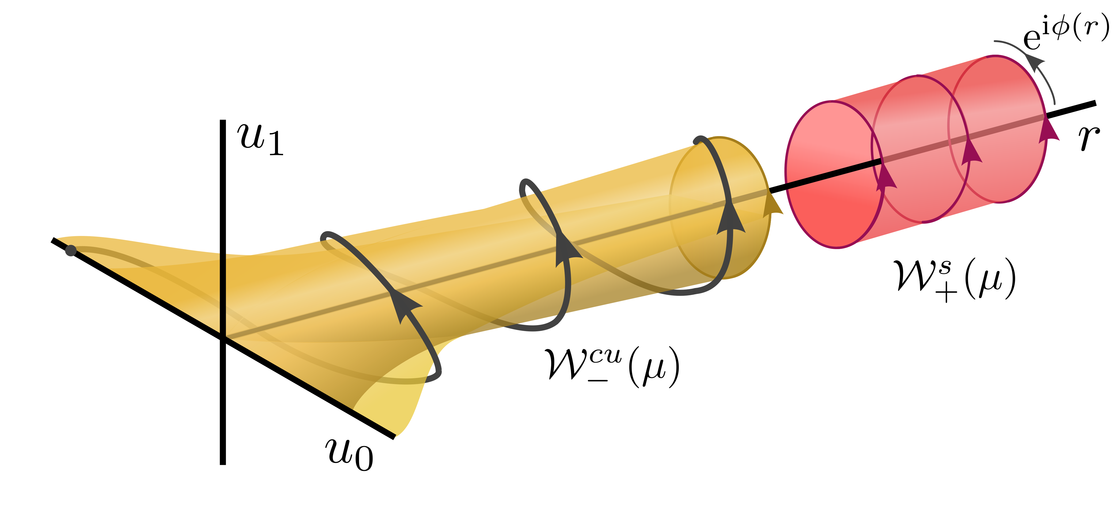
Figure 3: A diagram of the evolving shape of the core manifold $\mathcal{W}^{cu}_{-}(\mu)$ as $r$ increases, where $u_{i}:=\langle\hat{U}_{i}^{*},\mathbf{u}\rangle$ for $i=0,1$. The far-field manifold $\mathcal{W}^{s}_{+}(\mu)$ is constructed in a co-rotating frame with phase $\mathrm{e}^{\mathrm{i}\phi(r)}$.

We note that the core manifold $\mathcal{W}^{cu}_{-}(\mu)$ converges to a co-rotating two-dimensional manifold (3.21), with a co-rotating phase $\mathrm{e}^{\mathrm{i}(r_{0}-\frac{n\pi}{4})}$. We then expect the far-field manifold to possess a co-rotating phase $\mathrm{e}^{\mathrm{i}\phi(r)}$, where $\phi(r)$ is some perturbation from $(r-\frac{n\pi}{4})$; see Figure 3. We apply nonlinear normal form transformations to (3.20), as seen in [31, 22, 32], to remove the non-resonant terms from the right-hand side and the co-rotating phase $\mathrm{e}^{\mathrm{i}\phi(r)}$. For a more detailed proof of this result, see the analogous proof of Lemma 3.3 in Appendix A of [17].

Lemma 3.3.

There exists a change of coordinates

$$\begin{pmatrix}A\\ B\end{pmatrix}:=\textnormal{e}^{-\textnormal{i}\phi(r)}\left[\mathbbm{1}+\mathcal{T}(\sigma)\right]\begin{pmatrix}\widetilde{A}\\ \widetilde{B}\end{pmatrix}+\mathcal{O}((|\mu|+|\widetilde{A}|+|\widetilde{B}|)(|\widetilde{A}|+|\widetilde{B}|)),$$ (3.22)

such that (3.20) becomes

$$\begin{split}\frac{\textnormal{d}}{\textnormal{d}r}A&=-\frac{n}{2}\sigma A+B+R_{A}(A,B,\sigma,\mu),\\ \frac{\textnormal{d}}{\textnormal{d}r}B&=-\frac{n}{2}\sigma B+c_{0}\,\mu A+c_{3}|A|^{2}A+R_{B}(A,B,\sigma,\mu),\\ \frac{\textnormal{d}}{\textnormal{d}r}\sigma&=-\sigma^{2},\end{split}$$ (3.23)

where we recall from Hypothesis 2.1 that $c_{0}=\frac{1}{4}\big{\langle}\hat{U}_{1}^{*},-\mathbf{M}_{2}\hat{U}_{0}\big{\rangle}_{2}$ and

$$\begin{split}c_{3}={}&-\bigg{[}\bigg{(}\frac{5}{6}\big{[}\big{\langle}\hat{U}_{0}^{*},\mathbf{Q}_{0,0}\big{\rangle}_{2}+\big{\langle}\hat{U}_{1}^{*},\mathbf{Q}_{0,1}\big{\rangle}_{2}\big{]}+\frac{19}{18}\big{\langle}\hat{U}_{1}^{*},\mathbf{Q}_{0,0}\big{\rangle}_{2}\bigg{)}\big{\langle}\hat{U}_{1}^{*},\mathbf{Q}_{0,0}\big{\rangle}_{2}+\frac{3}{4}\big{\langle}\hat{U}_{1}^{*},\mathbf{C}_{0,0,0}\big{\rangle}_{2}\bigg{]}.\end{split}$$

The coordinate change (3.22) is polynomial in $(A,B,\sigma)$ and smooth in $\mu$, and $\mathcal{T}(\sigma)=\mathcal{O}(\sigma)$ is linear and upper triangular for each $\sigma$. The remainder terms satisfy

$$R_{A/B}=\mathcal{O}([|\mu|^{2}+|\sigma|^{3}+(|A|+|B|)^{2}]|B|+[|\mu|^{2}+|\sigma|^{3}+|A|^{3}]|A|),$$ (3.24)

while $\phi(r)$ satisfies

$$\frac{\textnormal{d}}{\textnormal{d}r}\phi=1+\mathcal{O}\left(|\mu|+|\sigma|^{2}\right),\qquad\phi(0)=0.$$

Having transformed our equations into the radial normal form (3.23) for an $n$-dimensional Hamiltonian–Hopf bifurcation, we also introduce the unconstrained variable $\kappa(r)$ to take the place of $\sqrt{\mu}$ so that the normal form (3.23) is extended to the following system,

$$\begin{split}\frac{\textnormal{d}}{\textnormal{d}r}A&=-\frac{n}{2}\sigma A+B+R_{A}(A,B,\sigma,\kappa),\\ \frac{\textnormal{d}}{\textnormal{d}r}B&=-\frac{n}{2}\sigma B+c_{0}\,\kappa^{2}A+c_{3}|A|^{2}A+R_{B}(A,B,\sigma,\kappa),\\ \frac{\textnormal{d}}{\textnormal{d}r}\sigma&=-\sigma^{2},\\ \frac{\textnormal{d}}{\textnormal{d}r}\kappa&=0\end{split}$$ (3.25)

where we have

$$R_{A/B}=\mathcal{O}([\kappa^{4}+|\sigma|^{3}+(|A|+|B|)^{2}]|B|+[\kappa^{4}+|\sigma|^{3}+|A|^{3}]|A|).$$ (3.26)

The remainder of this section is focused on characterising exponentially decaying trajectories for the dynamical system (3.25), restricted to the invariant subspace $\{(\sigma,\kappa)=(r^{-1},\sqrt{\mu})\}$. We characterise such trajectories for $r\geq r_{1}\mu^{-\frac{1}{2}}$ with $r_{1}\ll 1$ fixed (the rescaling chart, see § 3.3), and then for $r_{0}\leq r\leq r_{1}\mu^{-\frac{1}{2}}$ (the transition chart, see § 3.4). Following this, we seek intersections between the far-field trajectories and the core manifold $\mathcal{W}^{cu}_{-}(\mu)$ via asymptotic matching at the point $r=r_{0}$ (see § 3.5). Any trajectories that lie along these intersections will remain bounded as $r\to 0^{+}$ while decaying exponentially fast as $r\to\infty$, thus characterising localised radial solutions to (2.1).

The methods presented in the rest of this section are analogous to several previous studies of localised radial patterns, and so we present only condensed proofs of each result. For more detailed exposition on this approach, see [18, 26, 22, 16, 17].

3.3 The Rescaling Chart

We now define rescaling coordinates in order to find exponentially decaying solutions for sufficiently large values of $r$; that is, we introduce

$$A_{R}:=\kappa^{-1}A,\quad B_{R}:=\kappa^{-2}B,\quad\sigma_{R}:=\kappa^{-1}\sigma,\quad\kappa_{R}:=\kappa,\quad s:=\kappa r.$$ (3.27)

These coordinates are the standard rescaling coordinates seen in [26]. Then, we can write (3.25) in the rescaling chart as,

$$\begin{split}\frac{\textnormal{d}}{\textnormal{d}s}A_{R}&=-\frac{n}{2}\sigma_{R}A_{R}+B_{R}+|\kappa_{R}|^{-2}R_{A}(\kappa_{R}A_{R},\kappa^{2}_{R}B_{R},\kappa_{R}\sigma_{R},\kappa_{R}),\\ \frac{\textnormal{d}}{\textnormal{d}s}B_{R}&=-\frac{n}{2}\sigma_{R}B_{R}+c_{0}\,A_{R}+c_{3}|A_{R}|^{2}A_{R}+|\kappa_{R}|^{-3}R_{B}(\kappa_{R}A_{R},\kappa^{2}_{R}B_{R},\kappa_{R}\sigma_{R},\kappa_{R}),\\ \frac{\textnormal{d}}{\textnormal{d}s}\sigma_{R}&=-\sigma_{R}^{2},\\ \frac{\textnormal{d}}{\textnormal{d}s}\kappa_{R}&=0\end{split}$$ (3.28)

where

$$\begin{split}|\kappa_{R}|^{-2}R_{A}={}&|\kappa_{R}|^{2}\mathcal{O}([\kappa_{R}^{2}+|\kappa_{R}||\sigma_{R}|^{3}+(|A_{R}|+\kappa_{R}|B_{R}|)^{2}]|B_{R}|+[|\kappa_{R}|+|\sigma_{R}|^{3}+|A_{R}|^{3}]|A_{R}|),\\ |\kappa_{R}|^{-3}R_{B}={}&|\kappa_{R}|\mathcal{O}([\kappa_{R}^{2}+|\kappa_{R}||\sigma_{R}|^{3}+(|A_{R}|+\kappa_{R}|B_{R}|)^{2}]|B_{R}|+[|\kappa_{R}|+|\sigma_{R}|^{3}+|A_{R}|^{3}]|A_{R}|).\end{split}$$ (3.29)

Evaluating (3.28) on the invariant subspace $\{\sigma_{R}=s^{-1},\;\kappa_{R}=0\}$, we obtain the cubic nonautonomous complex Ginzburg–Landau equation

$$\mathcal{D}_{\frac{n}{2}}\mathcal{D}_{\frac{n}{2}}A_{R}(s)=c_{0}A_{R}(s)+c_{3}|A_{R}(s)|^{2}A_{R}(s),\qquad A_{R}\in\mathbb{C},\qquad s\in[0,\infty),$$ (3.30)

where, with a slight abuse of notation, we write $\mathcal{D}_{k}u(s)=(\frac{\mathrm{d}}{\mathrm{d}s}+\frac{k}{s})u(s)$ for any $k\in\mathbb{R}$. The equation (3.30) possesses $S^{1}$-symmetry, and so we reduce to the real subspace $A_{R}\in\mathbb{R}$ and consider solutions of the real Ginzburg–Landau equation

$$\mathcal{D}_{\frac{n}{2}}\mathcal{D}_{\frac{n}{2}}A_{R}(s)=c_{0}A_{R}(s)+c_{3}A_{R}(s)^{3},\qquad A_{R}\in\mathbb{R},\qquad s\in[0,\infty).$$ (3.31)

We present the following lemma regarding the existence of a nondegenerate solution to (3.31), which is required for the existence of ring and spot B solutions. We hence impose the restriction $0<n<4$, as required for such solutions in Therorem 2.8.

Lemma 3.4.

Fix $0<n<4$, assume that $c_{3}<0$. Then, the Ginzburg–Landau equation (3.31) has a forward-bounded localised solution $A_{R}(s)=\hat{q}(s):=|c_{3}|^{-\frac{1}{2}}\sqrt{c_{0}}q(\sqrt{c_{0}}s)$, with constants $q_{n}>0$, $p_{n}\neq 0$, which depend only on $n$, such that

$$q(s)=\begin{cases}q_{n}s^{\frac{2-n}{2}}\left(1+\mathcal{O}(s)\right),&s\to 0,\\ (p_{n}+\mathcal{O}(\mathrm{e}^{-s}))s^{-\frac{n}{2}}\mathrm{e}^{-s},&s\to\infty.\end{cases}$$ (3.32)

In addition, the linearisation of (3.31) about $\hat{q}(s)$ does not possess a nontrivial solution that is forward-bounded on $[0,\infty)$. If $c_{3}>0$, then the only forward-bounded solution of (3.31) on $[0,\infty)$ is $A_{R}(s)\equiv 0$.

Proof.

We begin by noting that bounded localised solutions of (3.31) must also satisfy

$$\begin{split}0={}&\int_{0}^{\infty}A_{R}(s)\left\{-\mathcal{D}_{\frac{n}{2}}\mathcal{D}_{\frac{n}{2}}A_{R}(s)+c_{0}A_{R}(s)+c_{3}|A_{R}(s)|^{2}A_{R}(s)\right\}\,s^{n}\,\mathrm{d}s\\ ={}&\int_{0}^{\infty}\left\{|\mathcal{D}_{\frac{n}{2}}A_{R}(s)|^{2}+c_{0}|A_{R}(s)|^{2}+c_{3}|A_{R}(s)|^{4}\right\}\,s^{n}\,\mathrm{d}s,\end{split}$$

and so we see that either $c_{3}<0$ or $A_{R}\equiv 0$. Assuming that $c_{3}<0$, we note that finding forward-bounded localised solutions to (3.31) is equivalent to finding radially-symmetric ground state solutions to

$$\Delta\hat{u}=\hat{u}-|\mathbf{x}|^{2-n}\hat{u}^{3},\qquad\hat{u}(\mathbf{x})\in\mathbb{R},\qquad\mathbf{x}\in\mathbb{R}^{3}.$$ (3.33)

where $\hat{u}(\mathbf{x})=|c_{3}|^{\frac{1}{2}}c_{0}^{\frac{n-4}{4}}|\mathbf{x}|^{\frac{n-2}{2}}A_{R}(c_{0}^{-\frac{1}{2}}|\mathbf{x}|)$. The key result here is that

$$\mathcal{D}_{\frac{n}{2}}\mathcal{D}_{\frac{n}{2}}\left(s^{\frac{2-n}{2}}u(s)\right)=s^{\frac{2-n}{2}}\mathcal{D}_{1}\mathcal{D}_{1}u(s)=s^{\frac{2-n}{2}}\Delta_{2}u(s)$$

which follows from the identities presented in (2.6). Hence the existence and non-degeneracy of $\hat{q}(s)$ follows from Proposition 2.7. Finally, the asymptotic behaviour of $q(s)$ in (3.32) can be found by noting that $q(s)$ is a solution of the rescaled equation

$$\mathcal{D}_{\frac{n}{2}}\mathcal{D}_{\frac{n}{2}}\hat{A}(s)=\hat{A}(s)-\hat{A}(s)^{3},$$ (3.34)

for which we can write down a variation-of-constants formula and apply a standard fixed-point argument in each limit. ∎

We note that spot A solutions do not persist as $\mathcal{O}(\mu^{\frac{1}{2}})$ perturbations from the localised solution in Lemma 3.4, but rather remain close to the linear flow of (3.31).

Remark 3.5.

For sufficiently small values of $A_{R}$, solutions of (3.31) remain close to exponentially decaying solutions of the linear equation

$$\mathcal{D}_{\frac{n}{2}}\mathcal{D}_{\frac{n}{2}}A_{R}(s)=c_{0}A_{R}(s),\qquad A_{R}\in\mathbb{R},\qquad s\in[0,\infty).$$ (3.35)

which have the explicit form $A_{R}(s)=s^{-\frac{n}{2}}\mathrm{e}^{-\sqrt{c_{0}}\,s}$.

We present the following lemma.

Lemma 3.6.

For each fixed choice of $r_{1}>0$, there are constants $a_{0},\kappa_{0}>0$ such that there exist exponentially decaying solutions to (3.28) for $s\in[r_{1},\infty)$, with the following evaluations at $s=r_{1}$ for all $\mu<\kappa_{0}$, $|a|<a_{0}$.

1. If $|A_{R}|=\mathcal{O}(a)$ as $|(a,\mu)|\to 0^{+}$, then

   $$(A_{R},B_{R},\sigma_{R},\kappa_{R})(r_{1})=\bigg{(}ar_{1}^{-\frac{n}{2}}A_{0},-\sqrt{c_{0}}ar_{1}^{-\frac{n}{2}}A_{0},r_{1}^{-1},\mu^{\frac{1}{2}}\bigg{)}.$$ (3.36)

2. If $c_{3}<0$, $n<4$ and $|A_{R}|=\mathcal{O}(1)$ as $|(a,\mu)|\to 0^{+}$, then

   $$(A_{R},B_{R},\sigma_{R},\kappa_{R})(r_{1})=\bigg{(}r_{1}^{\frac{2-n}{2}}\,A_{1},r_{1}^{-\frac{n}{2}}\,A_{1},r_{1}^{-1},\mu^{\frac{1}{2}}\bigg{)}.$$ (3.37)

   Here we have defined

   $$A_{0}:=\textnormal{e}^{\textnormal{i}Y}(1+\mathcal{O}(\mu^{\frac{1}{2}}+a^{2})),\qquad A_{1}:=|c_{3}|^{-\frac{1}{2}}c_{0}^{\frac{4-n}{4}}q_{n}\,\textnormal{e}^{\textnormal{i}Y}(1+\mathcal{O}(\mu^{\frac{1}{2}})),$$

   and $Y\in\mathbb{R}$ is arbitrary.

Proof.

We first note that $\kappa_{R}$ acts as a parameter, and $\Gamma_{c}:=\{(\sigma_{R},\kappa_{R})=(\tfrac{1}{s},\sqrt{c})\}$ is an invariant subspace of (3.28) for any fixed $c\geq 0$. Evaluating (3.28) on $\Gamma_{0}$, we arrive at the system

$$\begin{split}\mathcal{D}_{\frac{n}{2}}A_{R}(s)&=B_{R}(s),\\ \mathcal{D}_{\frac{n}{2}}B_{R}(s)&=c_{0}\,A_{R}(s)+c_{3}|A_{R}(s)|^{2}A_{R}(s),\\ \end{split}$$

which reduces to the complex cubic non-autonomous Ginzburg–Landau equation (3.30).

1. Assuming $|A_{R}|=\mathcal{O}(|a|)$ with $|a|\ll 1$ and recalling Remark 3.5, the equation (3.30) possesses an exponentially decaying solution for $s\in[r_{1},\infty)$ of the form

   $$\left(A_{R},B_{R},\sigma_{R},\kappa_{R}\right)(s)=\left(as^{-\frac{n}{2}}\mathrm{e}^{\sqrt{c_{0}}(r_{1}-s)}A_{0},-\sqrt{c_{0}}as^{-\frac{n}{2}}\mathrm{e}^{\sqrt{c_{0}}(r_{1}-s)}A_{0},s^{-1},\mu^{\frac{1}{2}}\right),$$ (3.38)

   for some $a\in\mathbb{R}$, $|a|\ll 1$, where the $\mathcal{O}(\mu^{\frac{1}{2}}+a^{2})$ terms are due to the $\mathcal{O}(|\kappa_{R}|)$ and $\mathcal{O}(|A_{R}|^{2}A_{R})$ terms in (3.28).

2. Assuming that $c_{3}<0$ and $n<4$, it follows from Lemma 3.4 that the equation (3.30) possesses an exponentially decaying solutions for $s\in[r_{1},\infty)$ of the form

   $$\left(A_{R},B_{R},\sigma_{R},\kappa_{R}\right)(s)=\left(\hat{q}(s)\,\mathrm{e}^{\mathrm{i}Y}(1+\mathcal{O}(\mu^{\frac{1}{2}})),\mathcal{D}_{\frac{n}{2}}\hat{q}(s)\,\mathrm{e}^{\mathrm{i}Y}(1+\mathcal{O}(\mu^{\frac{1}{2}})),\tfrac{1}{s},\mu^{\frac{1}{2}}\right),$$ (3.39)

   where the $\mathcal{O}(\mu^{\frac{1}{2}})$ terms are due to the $\mathcal{O}(|\kappa_{R}|)$ terms in (3.28).

Evaluating (3.38) and (3.39) at $s=r_{1}\ll 1$ and (in the case of $(ii)$) applying the asymptotic properties of $\hat{q}(s)=|c_{3}|^{-\frac{1}{2}}\sqrt{c_{0}}q(\sqrt{c_{0}}s)$ from (3.32), we arrive at our final result. ∎

We conclude this subsection by noting that upon inverting the rescaling transformation (3.27), exponentially decaying solutions to (3.25) evaluated at $r=r_{1}\mu^{-\frac{1}{2}}$ either take the form,

$$(A,B,\sigma,\kappa)(r_{1}\mu^{-\frac{1}{2}})=\bigg{(}a\mu^{\frac{1}{2}}r_{1}^{-\frac{n}{2}}A_{0},-\sqrt{c_{0}}a\mu r_{1}^{-\frac{n}{2}}A_{0},\mu^{\frac{1}{2}}r_{1}^{-1},\mu^{\frac{1}{2}}\bigg{)},$$ (3.40)

or, if $c_{3}<0$ and $n<4$,

$$(A,B,\sigma,\kappa)(r_{1}\mu^{-\frac{1}{2}})=\bigg{(}\mu^{\frac{1}{2}}r_{1}^{\frac{2-n}{2}}\,A_{1},\mu r_{1}^{-\frac{n}{2}}\,A_{1},\mu^{\frac{1}{2}}r_{1}^{-1},\mu^{\frac{1}{2}}\bigg{)},$$ (3.41)

for sufficiently small values of $a,\mu$.

3.4 The Transition Chart

In the previous subsection we parametrised the set of exponentially decaying solutions to (3.25) for $r>r_{1}\mu^{-\frac{1}{2}}$. Now, in order to match these exponentially decaying solutions with the core manifold described in §3.1, we must track the trajectories associated with (3.40) and (3.41) backwards through the ‘transition’ region $r_{0}\leq r\leq r_{1}\mu^{-\frac{1}{2}}$. This leads to the following result.

Lemma 3.7.

For each fixed choice of $0<r_{1},r_{0}^{-1}\ll 1$, there are constants $a_{0},\kappa_{0}>0$ such that solutions of (3.25), evaluated at $r=r_{0}$, $\kappa(r_{0})=\mu^{\frac{1}{2}}$, for initial values (3.40-3.41) are given by the following forms for all $\mu<\kappa_{0}$, $|a|<a_{0}$ and $Y\in\mathbb{R}$.

1. For initial value (3.40), we obtain a solution of the form

   $$\begin{split}A(r_{0})&=\mu^{\frac{2-n}{4}}r_{0}^{-\frac{n}{2}}a\mathrm{e}^{\mathrm{i}Y}(1+\xi_{0}),\\ B(r_{0})&=-\sqrt{c_{0}}\mu^{\frac{4-n}{4}}r_{0}^{-\frac{n}{2}}a\left[1+\frac{c_{3}}{\sqrt{c_{0}}}\frac{a^{2}}{\mathcal{E}^{2}_{n}(\mu)}\right]\mathrm{e}^{\mathrm{i}Y}(1+\xi_{0}).\\ \end{split}$$ (3.42)

2. For initial value (3.41) with $c_{3}<0$ and $n<4$, we obtain a solution of the form

   $$\begin{split}A(r_{0})&=|c_{3}|^{-\frac{1}{2}}c_{0}^{\frac{4-n}{4}}q_{n}\mu^{\frac{4-n}{4}}r_{0}^{\frac{2-n}{2}}\textnormal{e}^{\textnormal{i}Y}(1+\xi_{1}),\\ B(r_{0})&=|c_{3}|^{-\frac{1}{2}}c_{0}^{\frac{4-n}{4}}q_{n}\mu^{\frac{4-n}{4}}r_{0}^{-\frac{n}{2}}\textnormal{e}^{\textnormal{i}Y}(1+\xi_{1}).\\ \end{split}$$ (3.43)

3. Additionally, for initial value (3.41) with $c_{3}<0$ and $n<4$, we also obtain a solution of the form

   $$\begin{split}A(r_{0})&=a|c_{3}|^{-\frac{1}{2}}c_{0}^{\frac{4-n}{4}}q_{n}\mu^{\frac{4-n}{8}}r_{0}^{-\frac{n}{2}}\textnormal{e}^{\textnormal{i}Y}(1+\xi_{2}),\\ B(r_{0})&=|c_{3}|^{-\frac{1}{2}}c_{0}^{\frac{4-n}{4}}q_{n}\mu^{\frac{4-n}{4}}r_{0}^{-\frac{n}{2}}\textnormal{e}^{\textnormal{i}Y}(1+\xi_{2}).\\ \end{split}$$ (3.44)

Here we have defined the nonlinear function

$$\mathcal{E}_{n}(\mu):=\mu^{\frac{n-1}{4}}\left(\frac{(n-1)(\mu^{-\frac{1}{2}}r_{1})^{n-1}r_{0}^{n-1}}{\left(\mu^{-\frac{1}{2}}r_{1}\right)^{n-1}-r_{0}^{n-1}}\right)^{\frac{1}{2}}=\begin{cases}\mathcal{O}_{r_{0},r_{1}}(1),&0<n<1,\\ \mathcal{O}_{r_{0},r_{1}}(|\log(\mu)|^{-\frac{1}{2}}),&n=1,\\ \mathcal{O}_{r_{0},r_{1}}(\mu^{\frac{n-1}{4}}),&n>1,\\ \end{cases}$$

and introduced

$$\xi_{0}:=\mathcal{O}(\mu^{\frac{1}{2}}+a^{2}+r_{1}+r_{0}^{-1}),\qquad\xi_{1}:=\mathcal{O}(\mu^{\frac{1}{2}}+r_{1}+r_{0}^{-1}),\qquad\xi_{2}:=\mathcal{O}(\mu^{\frac{n}{2}}+\mu^{\frac{4-n}{8}}+|a|+r_{1}+r_{0}^{-1}),$$

for the remainder terms in (3.42-3.44).

Proof.

We begin by solving (3.25) for $\kappa(r)$ and $\sigma(r)$ explicitly, giving

$$\kappa(r)=\kappa\left(r_{1}\mu^{-\frac{1}{2}}\right)=\mu^{\frac{1}{2}},\quad\quad\sigma(r)=\frac{1}{\left(r-r_{1}\mu^{-\frac{1}{2}}\right)+\sigma\left(r_{1}\mu^{-\frac{1}{2}}\right)^{-1}}=\frac{1}{r}.$$

Our approach is then as follows. Given some fixed choice of $R_{-},R_{+}>0$ with $R_{-}<R_{+}$, we integrate backwards over $R_{-}\leq r\leq R_{+}$, such that (3.25) (evaluated at $\kappa=\mu^{\frac{1}{2}}$, $\sigma=\frac{1}{r}$) then becomes the integral equation

$$\begin{split}A(r)&=A(R_{+})+\int_{R_{+}}^{r}\left\{-\frac{n}{2p}A(p)+B(p)+R_{A}(A(p),B(p),p^{-1},\mu^{\frac{1}{2}})\right\}\,\mathrm{d}p,\\ B(r)&=B(R_{+})+\int_{R_{+}}^{r}\left\{-\frac{n}{2p}B(p)+c_{0}\,\mu A(p)+c_{3}|A(p)|^{2}A(p)+R_{B}(A(p),B(p),p^{-1},\mu^{\frac{1}{2}})\right\}\,\mathrm{d}p.\\ \end{split}$$ (3.45)

For sufficiently small values of $(A(R_{+}),B(R_{+}))$, we can apply the contraction mapping principle to show that (3.45) has a unique solution $(A,B)$ in an appropriate small ball centred at the origin in $C([R_{-},R_{+}],\mathbb{C}^{2})$; see, for example, [30]. Furthermore, we can express the unique solution to (3.45) evaluated at the point $r=R_{-}$ as a perturbation from $(A(R_{+}),B(R_{+}))$.

For each initial value (3.40, 3.41), we utilise this approach in conjunction with appropriate choices of $R_{-}$, $R_{+}$ and coordinate transformations for $(A,B)$ in order to obtain our expressions for $(A(r_{0}),B(r_{0}))$.

1. We begin by considering solutions with initial data (3.40). We introduce the following transition coordinates

   $$A_{T}:=r^{\frac{n}{2}}A,\qquad B_{T}:=r^{\frac{n}{2}}B,$$ (3.46)

   and integrate over $r_{0}\leq r\leq r_{1}\mu^{-\frac{1}{2}}$, so that (3.45) is replaced by

   $$\begin{split}A_{T}(r)&=a\mu^{\frac{2-n}{4}}A_{0}+\int_{r_{1}\mu^{-\frac{1}{2}}}^{r}\left\{B_{T}(p)+R_{A,T}(A_{T},B_{T};p,\mu^{\frac{1}{2}})\right\}\,\mathrm{d}p,\\ B_{T}(r)&=-\sqrt{c_{0}}a\mu^{\frac{4-n}{4}}A_{0}+\int_{r_{1}\mu^{-\frac{1}{2}}}^{r}\left\{c_{0}\,\mu A_{T}(p)+c_{3}p^{-n}|A_{T}(p)|^{2}A_{T}(p)+R_{B,T}(A_{T},B_{T};p,\mu^{\frac{1}{2}})\right\}\,\mathrm{d}p,\\ \end{split}$$

   where

   $$\begin{split}R_{A,T}(A_{T},B_{T};r,\mu^{\frac{1}{2}})={}&r^{\frac{n}{2}}R_{A}(r^{-\frac{n}{2}}A_{T},r^{-\frac{n}{2}}B_{T},r^{-1},\mu^{\frac{1}{2}}),\\ ={}&\mathcal{O}([\mu^{2}+r^{-3}+r^{-n}(|A_{T}|+|B_{T}|)^{2}]|B_{T}|+[\mu^{2}+r^{-3}+r^{-\frac{3n}{2}}|A_{T}|^{3}]|A_{T}|),\\ R_{B,T}(A_{T},B_{T};r,\mu^{\frac{1}{2}})={}&r^{\frac{n}{2}}R_{B}(r^{-\frac{n}{2}}A_{T},r^{-\frac{n}{2}}B_{T},r^{-1},\mu^{\frac{1}{2}}),\\ ={}&\mathcal{O}([\mu^{2}+r^{-3}+r^{-n}(|A_{T}|+|B_{T}|)^{2}]|B_{T}|+[\mu^{2}+r^{-3}+r^{-\frac{3n}{2}}|A_{T}|^{3}]|A_{T}|).\end{split}$$

   For sufficiently small values of $\mu$, we obtain a unique solution $(A_{T},B_{T})$ whose evaluation at the point $r=r_{0}$ has the following form

   $$A_{T}(r_{0})=\mu^{\frac{2-n}{4}}a\mathrm{e}^{\mathrm{i}Y}(1+\xi_{0}),\quad B_{T}(r_{0})=-\sqrt{c_{0}}\mu^{\frac{4-n}{4}}a\left[1+\frac{c_{3}}{\sqrt{c_{0}}}\frac{a^{2}}{\mathcal{E}_{n}(\mu)^{2}}\right]\mathrm{e}^{\mathrm{i}Y}(1+\xi_{0}).$$ (3.47)

   where we define $\mathcal{E}_{n}(\mu)$ such that

   $$\frac{1}{\mathcal{E}_{n}(\mu)^{2}}=\mu^{\frac{1-n}{2}}\int_{r_{1}\mu^{-\frac{1}{2}}}^{r_{0}}p^{-n}\,\mathrm{d}p=\frac{(r_{1}\mu^{-\frac{1}{2}})^{n-1}-r_{0}^{n-1}}{(n-1)(r_{0}r_{1})^{n-1}}.$$

2. We now consider solutions with initial values (3.41). We introduce the following transition coordinates

   $$\widetilde{A}_{T}:=r^{\frac{n-2}{2}}A,\qquad\widetilde{B}_{T}:=r^{\frac{n}{2}}B,$$ (3.48)

   and integrate over $r_{0}\leq r\leq r_{1}\mu^{-\frac{1}{2}}$, so that (3.45) is replaced by

   $$\begin{split}\widetilde{A}_{T}(r)&=\mu^{\frac{4-n}{4}}A_{1}+\int_{r_{1}\mu^{-\frac{1}{2}}}^{r}\left\{-p^{-1}\widetilde{A}_{T}(p)+p^{-1}\widetilde{B}_{T}(p)+R_{A,T}(\widetilde{A}_{T},\widetilde{B}_{T};p,\mu^{\frac{1}{2}})\right\}\,\mathrm{d}p,\\ \widetilde{B}_{T}(r)&=\mu^{\frac{4-n}{4}}A_{1}+\int_{r_{1}\mu^{-\frac{1}{2}}}^{r}\left\{c_{0}\,\mu p\widetilde{A}_{T}(p)+c_{3}p^{3-n}|\widetilde{A}_{T}(p)|^{2}\widetilde{A}_{T}(p)+R_{B,T}(\widetilde{A}_{T},\widetilde{B}_{T};p,\mu^{\frac{1}{2}})\right\}\,\mathrm{d}p.\\ \end{split}$$

   where

   $$\begin{split}R_{A,T}(\widetilde{A}_{T},\widetilde{B}_{T};r,\mu^{\frac{1}{2}})={}&r^{\frac{n-2}{2}}R_{A}(r^{\frac{2-n}{2}}\widetilde{A}_{T},r^{-\frac{n}{2}}\widetilde{B}_{T},r^{-1},\mu^{\frac{1}{2}}),\\ ={}&\mathcal{O}(r^{-1}[\mu^{2}+r^{-3}+r^{-n}(r|\widetilde{A}_{T}|+|\widetilde{B}_{T}|)^{2}]|\widetilde{B}_{T}|+[\mu^{2}+r^{-3}+r^{\frac{3(2-n)}{2}}|\widetilde{A}_{T}|^{3}]|\widetilde{A}_{T}|),\\ R_{B,T}(\widetilde{A}_{T},\widetilde{B}_{T};r,\mu^{\frac{1}{2}})={}&r^{\frac{n}{2}}R_{B}(r^{\frac{2-n}{2}}\widetilde{A}_{T},r^{-\frac{n}{2}}\widetilde{B}_{T},r^{-1},\mu^{\frac{1}{2}}),\\ ={}&\mathcal{O}([\mu^{2}+r^{-3}+r^{-n}(r|\widetilde{A}_{T}|+|\widetilde{B}_{T}|)^{2}]|\widetilde{B}_{T}|+r[\mu^{2}+r^{-3}+r^{\frac{3(2-n)}{2}}|\widetilde{A}_{T}|^{3}]|\widetilde{A}_{T}|).\end{split}$$

   For sufficiently small values of $\mu$, we obtain a unique solution $(\widetilde{A}_{T},\widetilde{B}_{T})$ whose evaluation at the point $r=r_{0}$ has the following form

   $$\widetilde{A}_{T}(r_{0})=|c_{3}|^{-\frac{1}{2}}c_{0}^{\frac{4-n}{4}}q_{n}\mu^{\frac{4-n}{4}}\textnormal{e}^{\textnormal{i}Y}(1+\xi_{1}),\quad\widetilde{B}_{T}(r_{0})=|c_{3}|^{-\frac{1}{2}}c_{0}^{\frac{4-n}{4}}q_{n}\mu^{\frac{4-n}{4}}\textnormal{e}^{\textnormal{i}Y}(1+\xi_{1}).$$ (3.49)

3. Finally, we consider solutions with initial values (3.41) which transition between $(\widetilde{A}_{T},\widetilde{B}_{T})$ and $(A_{T},B_{T})$ coordinates during their evolution in $r$, as observed in [26]. To do this we introduce some $a>0$ such that $r_{0}<a\mu^{-\frac{4-n}{8}}<r_{1}\mu^{-\frac{1}{2}}$. We then consider the transition coordinates $(\widetilde{A}_{T},\widetilde{B}_{T})$ as defined in (3.48) and integrate over $a\mu^{-\frac{4-n}{8}}\leq r\leq r_{1}\mu^{-\frac{1}{2}}$, so that (3.45) is replaced by

   $$\begin{split}\widetilde{A}_{T}(r)&=\mu^{\frac{4-n}{4}}A_{1}+\int_{r_{1}\mu^{-\frac{1}{2}}}^{r}\left\{-p^{-1}\widetilde{A}_{T}(p)+p^{-1}\widetilde{B}_{T}(p)+R_{A,T}(\widetilde{A}_{T},\widetilde{B}_{T};p,\mu^{\frac{1}{2}})\right\}\,\mathrm{d}p,\\ \widetilde{B}_{T}(r)&=\mu^{\frac{4-n}{4}}A_{1}+\int_{r_{1}\mu^{-\frac{1}{2}}}^{r}\left\{c_{0}\,\mu p\widetilde{A}_{T}(p)+c_{3}p^{3-n}|\widetilde{A}_{T}(p)|^{2}\widetilde{A}_{T}(p)+R_{B,T}(\widetilde{A}_{T},\widetilde{B}_{T};p,\mu^{\frac{1}{2}})\right\}\,\mathrm{d}p.\\ \end{split}$$

   As we saw previously, for sufficiently small values of $\mu$ we obtain a unique solution for $(\widetilde{A}_{T},\widetilde{B}_{T})$ whose evaluation at the point $r=a\mu^{-\frac{4-n}{8}}$ has the following form

   $$\widetilde{A}_{T}(a\mu^{-\frac{4-n}{8}})=\mu^{\frac{4-n}{4}}\widetilde{A}_{1},\quad\widetilde{B}_{T}(a\mu^{-\frac{4-n}{8}})=\mu^{\frac{4-n}{4}}\widetilde{A}_{1},$$ (3.50)

   where we have defined $\widetilde{A}_{1}:=|c_{3}|^{-\frac{1}{2}}c_{0}^{\frac{4-n}{4}}q_{n}\,\textnormal{e}^{\textnormal{i}Y}(1+\mathcal{O}(\mu^{\frac{4-n}{8}}+r_{1}))$. Transforming into the other transition coordinates $(A_{T},B_{T})$, defined in (3.46), and integrating over $r_{0}\leq r\leq a\mu^{-\frac{4-n}{8}}$, (3.45) is again replaced by

   $$\begin{split}A_{T}(r)&=a\mu^{\frac{4-n}{8}}\widetilde{A}_{1}+\int_{a\mu^{-\frac{4-n}{8}}}^{r}\left\{B_{T}(p)+R_{A,T}(A_{T},B_{T};p,\mu^{\frac{1}{2}})\right\}\,\mathrm{d}p,\\ B_{T}(r)&=\mu^{\frac{4-n}{4}}\widetilde{A}_{1}+\int_{a\mu^{-\frac{4-n}{8}}}^{r}\left\{c_{0}\,\mu A_{T}(p)+c_{3}p^{-n}|A_{T}(p)|^{2}A_{T}(p)+R_{B,T}(A_{T},B_{T};p,\mu^{\frac{1}{2}})\right\}\,\mathrm{d}p,\\ \end{split}$$

   Finally, for sufficiently small values of $\mu$ we obtain a unique solution for $(A_{T},B_{T})$ whose evaluation at the point $r=r_{0}$ has the following form

   $$A_{T}(r_{0})=a|c_{3}|^{-\frac{1}{2}}c_{0}^{\frac{4-n}{4}}q_{n}\mu^{\frac{4-n}{8}}\textnormal{e}^{\textnormal{i}Y}(1+\xi_{2}),\quad B_{T}(r_{0})=|c_{3}|^{-\frac{1}{2}}c_{0}^{\frac{4-n}{4}}q_{n}\mu^{\frac{4-n}{4}}\textnormal{e}^{\textnormal{i}Y}(1+\xi_{2}).$$ (3.51)

Inverting the transformations (3.46,3.48) brings us to the desired result. ∎

3.5 Matching Core and Far-field Manifolds

In the previous subsection we have obtained a parametrisation for exponentially-decaying trajectories of (3.18), which lie on the far-field manifold $\mathcal{W}^{s}_{+}(\mu)$, evaluated at the fixed point $r=r_{0}$. We now seek intersections of these trajectories with the parametrisation of the core manifold $\mathcal{W}^{cu}_{-}(\mu)$, evaluated at $r=r_{0}$, defined in (3.17).

We begin by applying (3.22) to the core parametrisation (3.21), such that the core manifold $\mathcal{W}^{cu}_{-}(\mu)$ can be expressed as

$$\begin{split}\widetilde{A}(r_{0})&=\frac{1}{2}r_{0}^{-\frac{n}{2}}\mathrm{e}^{\mathrm{i}Y_{n}}\left[d_{1}\left(1+\mathcal{O}(r_{0}^{-1})\right)-\mathrm{i}d_{2}r_{0}\left(1+\mathcal{O}(r_{0}^{-1})\right)+\mathcal{O}_{r_{0}}(|\mu||\mathbf{d}|+|\mathbf{d}|^{2})\right]\\ \widetilde{B}(r_{0})&=-\frac{1}{2}r_{0}^{-\frac{n}{2}}\mathrm{e}^{\mathrm{i}Y_{n}}\left[\gamma\,d_{1}^{2}\left(\nu_{n}+\mathcal{O}\left(r_{0}^{-\frac{n}{2}}+r_{0}^{-1}\right)\right)+\mathrm{i}d_{2}\left(1+\mathcal{O}(r_{0}^{-1})\right)+\mathcal{O}_{r_{0}}(|\mu||\mathbf{d}|+|d_{2}|^{2}+|d_{1}|^{3})\right]\\ \end{split}$$ (3.52)

where we recall $\nu_{n}=\left(\frac{3}{8}\right)^{\frac{n}{2}}\frac{\pi}{3\Gamma(\frac{n}{2})}$, $\gamma=\langle\hat{U}_{1}^{*},\mathbf{Q}(\hat{U}_{0},\hat{U}_{0})\rangle_{2}$ and introduce $Y_{n}=-\frac{n\pi}{4}+\mathcal{O}(|\mu|r_{0}+r_{0}^{-2})$.

Lemma 3.8.

For each fixed choice of $0<r_{1},r_{0}^{-1}\ll 1$, there is a constant $\kappa_{0}>0$ such that intersections between the core manifold (3.52) and respective far-field trajectories (3.42-3.44) satisfy the following conditions for all $\mu<\kappa_{0}$.

1. For (3.42) with $\gamma\neq 0$, we obtain $Y=Y_{n}$ and

   $$d_{1}=(c_{0}\mu)^{\frac{1}{2}}\frac{1}{\nu_{n}\gamma}\left(1+\mathcal{O}\left(r_{0}^{-1}+r_{1}+\mu^{\frac{1}{2}}+\mu^{\frac{n}{2}}\right)\right)\qquad d_{2}=\mu\,\mathcal{O}\left(r_{0}^{-1}+r_{1}+\mu^{\frac{1}{2}}+\mu^{\frac{n}{2}}\right).$$ (3.53)

2. For (3.42) with $\gamma=\mu^{\frac{n}{4}}\mathcal{E}_{n}(\mu)^{-1}\tilde{\gamma}$, we obtain $Y=Y_{n}$ and

   $$d_{1}=\frac{2\left[\nu_{n}\widetilde{\gamma}\,\pm\sqrt{\nu_{n}^{2}\widetilde{\gamma}^{2}-\sqrt{c_{0}}c_{3}}\right]}{c_{3}}\,\mu^{\frac{2-n}{4}}\mathcal{E}_{n}(\mu)\left(1+\mathrm{o}(1)\right),\qquad d_{2}=\mu^{\frac{4-n}{4}}\mathcal{E}_{n}(\mu)\,\mathrm{o}(1).$$ (3.54)

3. For (3.43) with $c_{3}<0$ and $n<4$, we obtain $Y=Y_{n}+(2\pm 1)\frac{\pi}{2}$ and

   $$d_{1}=\mu^{\frac{4-n}{4}}\mathcal{O}\left(r_{0}^{-1}+r_{1}+\mu^{\frac{1}{2}}+\mu^{\frac{4-n}{4}}\right),\qquad d_{2}=\pm\frac{2q_{n}}{\sqrt{|c_{3}|}}(c_{0}\mu)^{\frac{4-n}{4}}\left(1+\mathcal{O}\left(r_{0}^{-1}+r_{1}+\mu^{\frac{1}{2}}+\mu^{\frac{4-n}{4}}\right)\right).$$ (3.55)

4. For (3.44) with $c_{3}<0$ and $n<4$, we obtain $Y=Y_{n}+(\mathrm{sgn}(\gamma)-1)\frac{\pi}{2}$ and

   $$d_{1}=-\mathrm{sgn}(\gamma)\sqrt{\frac{2q_{n}}{\nu_{n}|\gamma|\sqrt{|c_{3}|}}}(c_{0}\mu)^{\frac{4-n}{8}}\,\left(1+\mathcal{O}(r_{0}^{-1}+r_{1}+\mu^{\frac{4-n}{8}})\right),\qquad d_{2}=\mu^{\frac{4-n}{4}}\mathcal{O}\left(r_{0}^{-1}+r_{1}+\mu^{\frac{4-n}{8}}\right).$$ (3.56)

Proof.

We consider each case separately:

1. Setting the far-field trajectory (3.42) and the core parametrisation (3.52) equal to each other, we look to solve

   $$\begin{split}2\mu^{\frac{2-n}{4}}a\mathrm{e}^{\mathrm{i}(Y-Y_{n})}(1+\xi_{0})={}&d_{1}\left(1+\mathcal{O}(r_{0}^{-1})\right)-\mathrm{i}d_{2}r_{0}\left(1+\mathcal{O}(r_{0}^{-1})\right)+\mathcal{O}_{r_{0}}(|\mu||\mathbf{d}|+|\mathbf{d}|^{2}),\\ 2\sqrt{c_{0}}\,g_{n}(a,\mu)\mathrm{e}^{\mathrm{i}(Y-Y_{n})}(1+\xi_{0})={}&\gamma\,d_{1}^{2}\left(\nu_{n}+\mathcal{O}\left(r_{0}^{-\frac{n}{2}}+r_{0}^{-1}\right)\right)+\mathrm{i}d_{2}\left(1+\mathcal{O}(r_{0}^{-1})\right)\\ &\hskip 108.405pt+\mathcal{O}_{r_{0}}(|\mu||\mathbf{d}|+|d_{2}|^{2}+|d_{1}|^{3}),\end{split}$$ (3.57)

   where $g_{n}(a,\mu):=\mu^{\frac{4-n}{4}}a(1+\frac{c_{3}}{\sqrt{c_{0}}}\mathcal{E}_{n}(\mu)^{-2}a^{2})$. We introduce the following coordinate transformations

   $$d_{1}=\sqrt{c_{0}}\mu^{\frac{1}{2}}\widetilde{d}_{1},\qquad d_{2}=c_{0}\mu\widetilde{d}_{2},\qquad a=\frac{\sqrt{c_{0}}}{2}\mu^{\frac{n}{4}}\widetilde{a},\qquad Y=Y_{n}+\widetilde{Y},$$ (3.58)

   so that (3.57) becomes

   $$\begin{split}\widetilde{a}\mathrm{e}^{\mathrm{i}\widetilde{Y}}(1+\xi_{0})={}&\widetilde{d}_{1}\left(1+\mathcal{O}(r_{0}^{-1})\right)+\mathcal{O}_{r_{0}}(\mu^{\frac{1}{2}}),\\ \widetilde{a}\mathrm{e}^{\mathrm{i}\widetilde{Y}}(1+\xi_{0})={}&\gamma\,\widetilde{d}_{1}^{2}\left(\nu_{n}+\mathcal{O}\left(r_{0}^{-\frac{n}{2}}+r_{0}^{-1}\right)\right)+\mathrm{i}\widetilde{d}_{2}\left(1+\mathcal{O}(r_{0}^{-1})\right)+\mathcal{O}_{r_{0}}(\mu^{\frac{1}{2}}+\mu^{\frac{n}{2}}\mathcal{E}_{n}(\mu)^{-2}).\end{split}$$ (3.59)

   We note that the final remainder term in (3.59) can be estimated by $\mathcal{O}_{r_{0}}(\mu^{\kappa})$ for some $\kappa>0$ for each choice of $n>0$ and, in particular,

   $$\mathcal{O}_{r_{0}}(\mu^{\frac{n}{2}}\mathcal{E}_{n}(\mu)^{-2})=\begin{cases}\mathcal{O}_{r_{0}}(\mu^{\frac{n}{2}}),&0<n<1,\\ \mathcal{O}_{r_{0}}(\mu^{\frac{1}{2}}|\log(\mu)|),&n=1,\\ \mathcal{O}_{r_{0}}(\mu^{\frac{1}{2}}),&n>1.\\ \end{cases}$$

   Then, taking $\mu,r_{1},r_{0}^{-1}\ll 1$, we obtain the leading-order system

   $$\begin{split}\widetilde{a}\mathrm{e}^{\mathrm{i}\widetilde{Y}}&=\widetilde{d}_{1},\qquad\widetilde{a}\mathrm{e}^{\mathrm{i}\widetilde{Y}}=\nu_{n}\widetilde{\gamma}\,\widetilde{d}_{1}^{2}+\mathrm{i}\widetilde{d}_{2}.\end{split}$$

   which has a solution of the form

   $$\widetilde{d}_{1}=\widetilde{a}=\frac{1}{\nu_{n}\gamma},\qquad\widetilde{d}_{2}=0,\qquad\widetilde{Y}=0.$$

2. In the case when $\gamma=\mu^{\frac{n}{4}}\mathcal{E}_{n}(\mu)^{-1}\tilde{\gamma}$, we instead introduce the following coordinate transformations

   $$d_{1}=\sqrt{c_{0}}\mu^{\frac{2-n}{4}}\mathcal{E}_{n}(\mu)\widetilde{d}_{1},\qquad d_{2}=c_{0}\mu^{\frac{4-n}{4}}\mathcal{E}_{n}(\mu)\widetilde{d}_{2},\qquad a=\frac{\sqrt{c_{0}}}{2}\mathcal{E}_{n}(\mu)\widetilde{a},\qquad Y=Y_{n}+\widetilde{Y},$$ (3.60)

   so that (3.57) becomes

   $$\begin{split}\widetilde{a}\mathrm{e}^{\mathrm{i}\widetilde{Y}}(1+\xi_{0})={}&\widetilde{d}_{1}\left(1+\mathcal{O}(r_{0}^{-1})\right)+\mathcal{O}_{r_{0}}(\mu^{\frac{1}{4}}),\\ \widetilde{a}\left[1+\frac{c_{3}\sqrt{c_{0}}}{4}\widetilde{a}^{2}\right]\mathrm{e}^{\mathrm{i}\widetilde{Y}}(1+\xi_{0})={}&\tilde{\gamma}\,\widetilde{d}_{1}^{2}\left(\nu_{n}+\mathcal{O}\left(r_{0}^{-\frac{n}{2}}+r_{0}^{-1}\right)\right)+\mathrm{i}\widetilde{d}_{2}\left(1+\mathcal{O}(r_{0}^{-1})\right)+\mathcal{O}_{r_{0}}(\mu^{\frac{1}{2}}).\end{split}$$ (3.61)

   Note, here we have estimated $\mathcal{O}_{r_{0}}(\mu^{\frac{2-n}{4}}\mathcal{E}_{n}(\mu))$ as $\mathcal{O}_{r_{0}}(\mu^{\frac{1}{4}})$, since

   $$\mathcal{O}_{r_{0}}(\mu^{\frac{2-n}{4}}\mathcal{E}_{n}(\mu))=\begin{cases}\mathcal{O}_{r_{0}}(\mu^{\frac{2-n}{4}}),&0<n<1,\\ \mathcal{O}_{r_{0}}(\mu^{\frac{1}{4}}|\log(\mu)|^{-\frac{1}{2}}),&n=1,\\ \mathcal{O}_{r_{0}}(\mu^{\frac{1}{4}}),&n>1.\\ \end{cases}$$

   Then, taking $0<\mu,r_{1},r_{0}^{-1}\ll 1$, we obtain the leading-order system

   $$\begin{split}\widetilde{a}\mathrm{e}^{\mathrm{i}\widetilde{Y}}&=\widetilde{d}_{1},\\ \widetilde{a}\left[1+\frac{\sqrt{c_{0}}c_{3}}{4}\widetilde{a}^{2}\right]\mathrm{e}^{\mathrm{i}\widetilde{Y}}&=\nu_{n}\widetilde{\gamma}\,\widetilde{d}_{1}^{2}+\mathrm{i}\widetilde{d}_{2},\end{split}$$

   which has solutions of the form

   $$\widetilde{d}_{1}=\widetilde{a}=\frac{2\left[\nu_{n}\widetilde{\gamma}\,\pm\sqrt{\nu_{n}^{2}\widetilde{\gamma}^{2}-\sqrt{c_{0}}c_{3}}\right]}{\sqrt{c_{0}}c_{3}},\qquad\widetilde{d}_{2}=0,\qquad\widetilde{Y}=0.$$ (3.62)

3. Setting the far-field trajectory (3.43) and the core parametrisation (3.52) equal to each other, we look to solve

   $$\begin{split}2q_{n}\mu^{\frac{4-n}{4}}r_{0}\textnormal{e}^{\textnormal{i}(Y-Y_{n})}(1+\xi_{1})&=d_{1}\left(1+\mathcal{O}(r_{0}^{-1})\right)-\mathrm{i}d_{2}r_{0}\left(1+\mathcal{O}(r_{0}^{-1})\right)+\mathcal{O}_{r_{0}}(|\mu||\mathbf{d}|+|\mathbf{d}|^{2}),\\ 2q_{n}\mu^{\frac{4-n}{4}}\textnormal{e}^{\textnormal{i}(Y-Y_{n})}(1+\xi_{1})&=-\gamma\,d_{1}^{2}\left(\nu_{n}+\mathcal{O}\left(r_{0}^{-\frac{n}{2}}+r_{0}^{-1}\right)\right)-\mathrm{i}d_{2}\left(1+\mathcal{O}(r_{0}^{-1})\right)\\ &\hskip 151.76964pt+\mathcal{O}_{r_{0}}(|\mu||\mathbf{d}|+|d_{2}|^{2}+|d_{1}|^{3}).\end{split}$$ (3.63)

   We introduce the following coordinate transformations

   $$d_{1}=2q_{n}\mu^{\frac{4-n}{4}}r_{0}\widetilde{d}_{1},\qquad d_{2}=2q_{n}\mu^{\frac{4-n}{4}}\widetilde{d}_{2},\qquad Y=Y_{n}+\widetilde{Y},$$ (3.64)

   so that (3.63) becomes

   $$\begin{split}\textnormal{e}^{\textnormal{i}\widetilde{Y}}(1+\xi_{1})&=\widetilde{d}_{1}\left(1+\mathcal{O}(r_{0}^{-1})\right)-\mathrm{i}\widetilde{d}_{2}\left(1+\mathcal{O}(r_{0}^{-1})\right)+\mathcal{O}_{r_{0}}(\mu^{\frac{4-n}{4}}),\\ \textnormal{e}^{\textnormal{i}\widetilde{Y}}(1+\xi_{1})&=-\mathrm{i}\widetilde{d}_{2}\left(1+\mathcal{O}(r_{0}^{-1})\right)+\mathcal{O}_{r_{0}}(\mu^{\frac{4-n}{4}}).\end{split}$$ (3.65)

   Then, taking $0<\mu,r_{1},r_{0}^{-1}\ll 1$, we obtain the leading-order system

   $$\begin{split}\textnormal{e}^{\textnormal{i}\widetilde{Y}}&=\widetilde{d}_{1}-\mathrm{i}\widetilde{d}_{2},\qquad\textnormal{e}^{\textnormal{i}\widetilde{Y}}=-\mathrm{i}\widetilde{d}_{2}.\end{split}$$

   which has solutions of the form

   $$\widetilde{d}_{1}=0,\qquad\widetilde{d}_{2}=\pm 1,\qquad\widetilde{Y}=\frac{(2\pm 1)\pi}{2}.$$

4. Setting the far-field trajectory (3.44) and the core parametrisation (3.52) equal to each other, we look to solve

   $$\begin{split}2aq_{n}\mu^{\frac{4-n}{8}}\textnormal{e}^{\textnormal{i}(Y-Y_{n})}(1+\xi_{2})&=d_{1}\left(1+\mathcal{O}(r_{0}^{-1})\right)-\mathrm{i}d_{2}r_{0}\left(1+\mathcal{O}(r_{0}^{-1})\right)+\mathcal{O}_{r_{0}}(|\mu||\mathbf{d}|+|\mathbf{d}|^{2}),\\ 2q_{n}\mu^{\frac{4-n}{4}}\textnormal{e}^{\textnormal{i}(Y-Y_{n})}(1+\xi_{2})&=-\gamma\,d_{1}^{2}\left(\nu_{n}+\mathcal{O}\left(r_{0}^{-\frac{n}{2}}+r_{0}^{-1}\right)\right)-\mathrm{i}d_{2}\left(1+\mathcal{O}(r_{0}^{-1})\right)\\ &\hskip 151.76964pt+\mathcal{O}_{r_{0}}(|\mu||\mathbf{d}|+|d_{2}|^{2}+|d_{1}|^{3}).\end{split}$$ (3.66)

   We introduce the following coordinate transformations

   $$d_{1}=\mu^{\frac{4-n}{8}}\widetilde{d}_{1},\qquad d_{2}=\mu^{\frac{4-n}{4}}\widetilde{d}_{2},\qquad Y=Y_{n}+\widetilde{Y},$$ (3.67)

   so that (3.66) becomes

   $$\begin{split}2aq_{n}\textnormal{e}^{\textnormal{i}\widetilde{Y}}(1+\xi_{2})&=\widetilde{d}_{1}\left(1+\mathcal{O}(r_{0}^{-1})\right)+\mathcal{O}_{r_{0}}(\mu^{\frac{4-n}{8}}),\\ 2q_{n}\textnormal{e}^{\textnormal{i}\widetilde{Y}}(1+\xi_{2})&=-\gamma\,\widetilde{d}_{1}^{2}\left(\nu_{n}+\mathcal{O}\left(r_{0}^{-\frac{n}{2}}+r_{0}^{-1}\right)\right)-\mathrm{i}\widetilde{d}_{2}\left(1+\mathcal{O}(r_{0}^{-1})\right)+\mathcal{O}_{r_{0}}(\mu^{\frac{4-n}{4}}).\end{split}$$ (3.68)

   Then, taking $0<\mu,r_{1},r_{0}^{-1}\ll 1$, we obtain the leading-order system

   $$\begin{split}2aq_{n}\textnormal{e}^{\textnormal{i}\widetilde{Y}}=\widetilde{d}_{1},\qquad 2q_{n}\textnormal{e}^{\textnormal{i}\widetilde{Y}}=-\nu_{n}\gamma\widetilde{d}_{1}^{2}-\mathrm{i}\widetilde{d}_{2},\end{split}$$

   which has a solution of the form

   $$\widetilde{d}_{1}=-\mathrm{sgn}(\gamma)\sqrt{\frac{2q_{n}}{\nu_{n}|\gamma|}},\qquad\widetilde{d}_{2}=0,\qquad a=\sqrt{\frac{1}{2q_{n}\nu_{n}|\gamma|}},\qquad\widetilde{Y}=\frac{(\mathrm{sgn}(\gamma)-1)\pi}{2}.$$

Having determined the leading order solution in each case, we now apply the implicit function theorem to solve (3.59, 3.61, 3.65, 3.68) uniquely for all $0<\mu,r_{1},r_{0}^{-1}\ll 1$. Inverting the respective coordinate transformations (3.58, 3.60, 3.64, 3.67), we arrive at our result. ∎

4 Discussion

In this paper, we have proven that localised $(n+1)$-dimensional radial patterns emerge from non-degenerate Turing bifurcations in general two-component reaction-diffusion systems. Extending the approach of [22, 26], we determined that spot A patterns emerge for all values of the dimension parameter $n>0$, where the core profile depends continuously on $n$ and possesses a fixed asymptotic scaling $\mu^{\frac{1}{2}}$. In contrast, we found that ring and spot B patterns only emerge for $0<n<4$, where their core profiles depend continuously on $n$ and they possess an asymptotic scaling $\mu^{\frac{4-n}{4}}$, $\mu^{\frac{4-n}{8}}$, respectively. The core profile for each pattern depends on $(n+1)$-dimensional Bessel functions $J^{(n)}_{\ell}(r)$, which can be written in terms of standard Bessel functions; this highlights the connection between core profiles of two-dimensional and three-dimensional radial patterns that was previously unclear. Our results agree with previous findings in [22, 26], while providing a proof for the previously unproven existence of three-dimensional rings and presenting simplified proofs for spot B patterns and solutions of the non-autonomous Ginzburg–Landau equation (3.30).

We briefly discuss the intuition behind the asymptotic scaling $\mu^{\frac{4-n}{4}}$ for localised rings and the corresponding requirement that $0<n<4$. As mentioned previously, this scaling was predicted in [26] through a formal analysis, however the intuition for this scaling was not explored further. In the derivation for localised ring patterns $\mathbf{u}_{R}(r)$, we seek solutions that satisfy the far-field scaling $|\mathbf{u}_{R}(r)|=\mathcal{O}(\mu^{\frac{1}{2}})$ when $r=\mathcal{O}(\mu^{-\frac{1}{2}})$. If we suppose that our solution satisfies $|\mathbf{u}_{R}(r)|=\mathcal{O}(\mu^{\alpha}\,|rJ_{1}^{(n)}(r)|)$ for some $\alpha>0$, then (using Table 1) $|\mathbf{u}_{R}(r)|=\mathcal{O}(\mu^{\alpha}\,r^{\frac{2-n}{2}})$ for large values of $r$. Furthermore, for $r=\mathcal{O}(\mu^{-\frac{1}{2}})$ we obtain $|\mathbf{u}_{R}(r)|=\mathcal{O}(\mu^{\alpha+\frac{n-2}{4}})$ and so rings must satisfy $\alpha+\frac{n-2}{4}=\frac{1}{2}$. Hence, the far-field profile is always smaller than $\mathcal{O}(\mu^{\frac{1}{2}})$ if $n>4$. We note that localised rings may still emerge for $n>4$, except they will not satisfy the standard far-field scaling. Instead, localised patterns with the form $|\mathbf{u}(r)|=\mathcal{O}(\mu^{\alpha}\,|rJ_{1}^{(n)}(r)|)$ for $n>4$, either must satisfy $|\mathbf{u}(r)|=\mathcal{O}(\mu^{\kappa})$ with $\kappa>\frac{1}{2}$ in the region $r=\mathcal{O}(\mu^{-\frac{1}{2}})$, or $|\mathbf{u}(r)|=\mathcal{O}(\mu^{\frac{1}{2}})$ in the region $r=\mathcal{O}(\mu^{-\beta})$ with $\beta<\frac{1}{2}$. We leave this approach for future study.

While we have considered the emergence of localised radial patterns from an $(n+1)$-dimensional Turing instability, very little is understood of their behaviour away from this bifurcation point. As seen in Figure 1(a), spot A patterns may undergo snaking behaviour as they move away from their bifurcation point. This is behaviour is known as homoclinic snaking (first introduced in [40]) when $n=0$, which has been the subject of over two decades of research, (see [9]) but is still not well-understood for $n>0$. While there has been some numerical studies of the bifurcation structure of spots in two and three dimensions [25, 13], and analytical results regarding ring patterns in $n$-spatial dimensions [6], this topic still requires further investigation.

A natural next step in this analysis would be to consider the stability of localised radial patterns for various spatial dimensions. In particular, the transition of localised one-dimensional patterns to axisymmetric patterns (and from axisymmetric to spherically-symmetric) would be an interesting phenomenon to explore. Our current approach could also be extended to higher-dimensional symmetries, such as the dihedral patterns considered in [16, 17]. This would require some kind of formulation of $(n+1)$-dimensional spherical harmonics that vary continuously with respect to $n$. Being able to describe the transition of more general patterns into their higher- or lower-dimensional counterparts would an extremely powerful tool for understanding pattern formation in nature.

• Acknowledgments. The author gratefully acknowledges support from the Alexander von Humboldt foundation, and would like to thank David Lloyd for his comments on an earlier draft of this manuscript.

References

- [1] M. Abramowitz and I. Stegun. Handbook of Mathematical Functions with Formulas, Graphs, and Mathematical Tables. Dover, New York, 1972.
- [2] M. Alber, T. Glimm, H. G. E. Hentschel, B. Kazmierczak, and S. A. Newman. Stability of n-dimensional patterns in a generalized turing system: implications for biological pattern formation. Nonlinearity, 18(1):125, oct 2004.
- [3] L. J. S. Allen, B. M. Bolker, Y. Lou, and A. L. Nevai. Asymptotic profiles of the steady states for an SIS epidemic reaction-diffusion model. Discrete and Continuous Dynamical Systems, 21(1):1–20, 2008.
- [4] J. Avery and J. Avery. Generalized Sturmians And Atomic Spectra. World Scientific Publishing Company, 2006.
- [5] D. Avitabile. Numerical Computation of Coherent Structures in Spatially-Extended Systems, may 2020.
- [6] J. J. Bramburger, D. Altschuler, C. I. Avery, T. Sangsawang, M. Beck, P. Carter, and B. Sandstede. Localized radial roll patterns in higher space dimensions. SIAM Journal on Applied Dynamical Systems, 18(3):1420–1453, 2019.
- [7] J. J. Bramburger, D. J. Hill, and D. J. B. Lloyd. Localized multi-dimensional patterns, 2024. arXiv preprint.
- [8] T. Bánsági, V. K. Vanag, and I. R. Epstein. Tomography of reaction-diffusion microemulsions reveals three-dimensional turing patterns. Science, 331(6022):1309–1312, 2011.
- [9] A. Champneys. Editorial to Homoclinic snaking at 21: in memory of Patrick Woods. IMA Journal of Applied Mathematics, 86(5):845–855, 10 2021.
- [10] S.-M. Chang, S. Gustafson, K. Nakanishi, and T.-P. Tsai. Spectra of linearized operators for NLS solitary waves. SIAM Journal on Mathematical Analysis, 39(4):1070–1111, 2008.
- [11] M. G. Clerc, S. Echeverría-Alar, and M. Tlidi. Localised labyrinthine patterns in ecosystems. Scientific Reports, 11(1):18331, Sep 2021.
- [12] W.-Y. Ding and W.-M. Ni. On the existence of positive entire solutions of a semilinear elliptic equation. Archive for Rational Mechanics and Analysis, 91(4):283–308, Dec 1986.
- [13] D. Gomila and E. Knobloch. Curvature effects and radial homoclinic snaking. IMA Journal of Applied Mathematics, 86(5):1094–1111, 08 2021.
- [14] M. D. Groves and D. J. Hill. On function spaces for radial functions, 2024. arXiv preprint.
- [15] D. J. Hill. Existence of localized radial patterns in a model for dryland vegetation. IMA Journal of Applied Mathematics, 87(3):315–353, 05 2022.
- [16] D. J. Hill, J. J. Bramburger, and D. J. B. Lloyd. Approximate localised dihedral patterns near a Turing instability. Nonlinearity, 36(5):2567, 2023.
- [17] D. J. Hill, J. J. Bramburger, and D. J. B. Lloyd. Dihedral rings of patterns emerging from a turing bifurcation. Nonlinearity, 37(3):035015, feb 2024.
- [18] D. J. Hill, D. J. B. Lloyd, and M. R. Turner. Localised radial patterns on the surface of a ferrofluid. J. Nonlinear Sci., 31(79), 2021.
- [19] T. J. Jewell, A. L. Krause, P. K. Maini, and E. A. Gaffney. Patterning of nonlocal transport models in biology: The impact of spatial dimension. Mathematical Biosciences, 366:109093, 2023.
- [20] P. Lions. The concentration-compactness principle in the calculus of variations. the locally compact case, part 1. Annales de l’Institut Henri Poincaré C, Analyse non linéaire, 1(2):109–145, 1984.
- [21] P. Lions. The concentration-compactness principle in the calculus of variations. the locally compact case, part 2. Annales de l’Institut Henri Poincaré C, Analyse non linéaire, 1(4):223–283, 1984.
- [22] D. Lloyd and B. Sandstede. Localized radial solutions of the Swift-Hohenberg equation. Nonlinearity, 22(2):485–524, 2009.
- [23] D. Lloyd, B. Sandstede, D. Avitabile, and A. Champneys. Localized hexagon patterns of the planar Swift-Hohenberg equation. SIAM J. Appl. Dyn. Syst., 7(3):1049–1100, 2008.
- [24] L. A. Lugiato and R. Lefever. Spatial dissipative structures in passive optical systems. Phys. Rev. Lett., 58:2209–2211, May 1987.
- [25] S. McCalla and B. Sandstede. Snaking of radial solutions of the multi-dimensional swift–hohenberg equation: A numerical study. Physica D: Nonlinear Phenomena, 239(16):1581–1592, 2010.
- [26] S. McCalla and B. Sandstede. Spots in the Swift-Hohenberg equation. SIAM J. Appl. Dyn. Syst., 12(2):831–877, 2013.
- [27] J. McSloy, W. Firth, G. Harkness, and G.-L. Oppo. Computationally determined existence and stability of transverse structures. II. Multipeaked cavity solitons. Physical Review E, 66(4):046606, 2002.
- [28] Y. Menesguen, S. Barbay, X. Hachair, L. Leroy, I. Sagnes, and R. Kuszelewicz. Optical self-organization and cavity solitons in optically pumped semiconductor microresonators. Physical Review A, 74(2):023818, 2006.
- [29] E. Meron, H. Yizhaq, and E. Gilad. Localized structures in dryland vegetation: Forms and functions. Chaos: An Interdisciplinary Journal of Nonlinear Science, 17(3):037109, 2007.
- [30] B. Sandstede. Convergence estimates for the numerical approximation of homoclinic solutions. IMA J. Numer. Anal., 17(3):437–462, 1997.
- [31] A. Scheel. Radially symmetric patterns of reaction-diffusion systems. Mem. Amer. Math. Soc., 165(786):viii+86, 2003.
- [32] A. Scheel and Q. Wu. Small-amplitude grain boundaries of arbitrary angle in the Swift-Hohenberg equation. Z. Angew. Math. Mech., 94(3):203–232, 2014.
- [33] C. Stuart. Bifurcation for variational problems when the linearisation has no eigenvalues. Journal of Functional Analysis, 38(2):169–187, 1980.
- [34] M. Tlidi, S. Gopalakrishnan, M. Taki, and K. Panajotov. Optical crystals and light-bullets in Kerr resonators. Chaos, Solitons & Fractals, 152:111364, 2021.
- [35] J. van den Berg, C. Groothedde, and J. Williams. Rigorous computation of a radially symmetric localized solution in a Ginzburg-Landau problem. SIAM J. Appl. Dyn. Syst., 14(1):423–447, 2015.
- [36] R. A. Van Gorder, V. Klika, and A. L. Krause. Turing conditions for pattern forming systems on evolving manifolds. Journal of Mathematical Biology, 82(1):4, Jan 2021.
- [37] V. K. Vanag and I. R. Epstein. Stationary and oscillatory localized patterns, and subcritical bifurcations. Physical Review letters, 92(12):128301, 2004.
- [38] J. von Hardenberg, E. Meron, M. Shachak, and Y. Zarmi. Diversity of vegetation patterns and desertification. Physical Review Letters, 87:198101, 2001.
- [39] Z. Wen and J. Avery. Some properties of hyperspherical harmonics. Journal of Mathematical Physics, 26(3):396–403, 03 1985.
- [40] P. Woods and A. Champneys. Heteroclinic tangles and homoclinic snaking in the unfolding of a degenerate reversible hamiltonian–hopf bifurcation. Physica D: Nonlinear Phenomena, 129(3):147–170, 1999.
- [41] Y. R. Zelnik, E. Meron, and G. Bel. Gradual regime shifts in fairy circles. Proceedings of the National Academy of Sciences, 112(40):12327–12331, 2015.