Demystifying amortized causal discovery with transformers

Abstract

Supervised learning approaches for causal discovery from observational data often achieve competitive performance despite seemingly avoiding explicit assumptions that traditional methods make for identifiability. In this work, we investigate CSIvA [1], a transformer-based model promising to train on synthetic data and transfer to real data. First, we bridge the gap with existing identifiability theory and show that constraints on the training data distribution implicitly define a prior on the test observations. Consistent with classical approaches, good performance is achieved when we have a good prior on the test data, and the underlying model is identifiable. At the same time, we find new trade-offs. Training on datasets generated from different classes of causal models, unambiguously identifiable in isolation, improves the test generalization. Performance is still guaranteed, as the ambiguous cases resulting from the mixture of identifiable causal models are unlikely to occur (which we formally prove). Overall, our study finds that amortized causal discovery still needs to obey identifiability theory, but it also differs from classical methods in how the assumptions are formulated, trading more reliance on assumptions on the noise type for fewer hypotheses on the mechanisms.

1 Introduction

Causal discovery aims to uncover the underlying causal relationships between variables of a system from pure observations, which is crucial for answering interventional and counterfactual queries when experimentation is impractical or unfeasible [2, 3, 4]. Unfortunately, causal discovery is inherently ill-posed [5]: unique identification of causal directions requires restrictive assumptions on the class of structural causal models (SCMs) that generated the data [6, 7, 8]. These theoretical limitations often render existing methods inapplicable, as the underlying assumptions are usually untestable or difficult to verify in practice [9].

Recently, supervised learning algorithms trained on synthetic data have been proposed to overcome the need for specific hypotheses, which restrains the application of classical causal discovery methods to real-world problems [1, 10, 11, 12, 13]. Seminal work from Lopez-Paz et al. [10] argues that this learning-based approach to causal discovery would allow dealing with complex data-generating processes and would greatly reduce the need for explicitly crafting identifiability conditions a-priori: despite this ambitious goal, the output of these methods is generally considered unreliable, as no theoretical guarantee is provided. A pair of non-identifiable structural causal models can be associated with different causal graphs $\mathcal{G}\neq\tilde{\mathcal{G}}$, while entailing the same joint distribution $p$ on the system’s variables. It is thus unclear how a learning algorithm presented with observational data generated from $p$ would be able to overcome these theoretical limits and correctly identify a unique causal structure. However, the available empirical evidence seems not to care about impossibility results, as these methods yield surprising generalization results on several synthetic benchmarks. Our work aims to bridge this gap by studying the performance of a transformer architecture for causal discovery through the lens of the theory of identifiability from observational data. Specifically, we analyze the CSIvA (Causal Structure Induction via Attention) model for causal discovery [1], focusing on bivariate graphs, as they offer a controlled yet non-trivial setting for the investigation. As our starting point, we provide closed-form examples that identify the limitations of CSIvA in recovering causal structures of linear non-Gaussian and nonlinear additive noise models, which are notably identifiable, and demonstrate the expected failures through empirical evidence. These findings suggest that the class of structural causal models that can be identified by CSIvA is inherently dependent on the specific class of SCMs observed during training. Thus, the need for restrictive hypotheses on the data-generating process is intrinsic to causal discovery, both in the traditional and modern learning-based approaches: assumptions on the test distribution either are posited when selecting the algorithm (traditional methods) or in the choice of the training data (learning-based methods). To address this limitation, we theoretically and empirically analyze when training CSIvA on datasets generated by multiple identifiable SCMs with different structural assumptions improves its generalization at test time. In summary:

• We show that the class of structural causal models that CSIvA can identify is defined by the class of SCMs observed through samples during the training. We reinforce the notion that identifiability in causal discovery inherently requires assumptions, which must be encoded in the training data in the case of learning-based approaches.

• To overcome this limitation, we study the benefits of CSIvA training on mixtures of causal models. We analyze when algorithms learned on multiple models are expected to identify broad classes of SCMs (unlike many classical methods). Empirically, we show that training on samples generated by multiple identifiable causal models with different assumptions on mechanisms and noise distribution results in significantly improved generalization abilities.

Closely related works and their relation with CSIvA.

In this paper, we study amortized inference of causal graphs, i.e. optimization of an inference model to directly predict a causal structure from newly provided data. This is the first work that attempts to understand the connection between identifiability theory and amortized inference, while several algorithms have been proposed. In the context of purely observational data, Lopez-Paz et al. [10] defines a distribution regression problem [14] mapping the kernel mean embedding of the data distribution to a causal graph, while Li et al. [11] relies on equivariant neural network architectures. More recently, Lippe et al. [12] and Lorch et al. [13] proposed learning on interventional data, in addition to observations (in the same spirit as CSIvA). Despite different algorithmic implementations, the target object of estimation of most of these methods is the distribution over the space of all possible graphs, conditional on the input dataset (similarly, the ENCO algorithm in Lippe et al. [12] models the conditional distribution of individual edges). This justifies our choice of restricting our study to the CSIvA architecture (despite this being a clear limitation), as in the infinite observational sample limit, these methods approximate the same distribution. Methods necessarily requiring interventional data [15, 16, 17], and learning-based algorithms unsuitable for amortized inference [18, 19, 20, 21, 22] are out of the scope of this work.

2 Background and motivation

We start introducing structural causal models (SCMs), an intuitive framework that formalizes causal relations. Let $X$ be a set of random variables in $\mathbb{R}$ defined according to the set of structural equations:

$$X_{i}\coloneqq f_{i}(X_{\operatorname{PA}^{\mathcal{G}}_{i}},N_{i}),\hskip 5.69054pt\forall i=1,\ldots,k.$$ (1)

$N_{i}\in\mathbb{R}$ are noise random variables. The function $f_{i}$ is the causal mechanism mapping the set of direct causes $X_{\operatorname{PA}^{\mathcal{G}}_{i}}$ of $X_{i}$ and the noise term $N_{i}$, to $X_{i}$’s value. The causal graph $\mathcal{G}$ is a directed acyclic graph (DAG) with nodes $X=\{X_{1},\ldots,X_{k}\}$, and edges $\{X_{j}\rightarrow X_{i}:X_{j}\in X_{\operatorname{PA}^{\mathcal{G}}_{i}}\}$, with $\operatorname{PA}^{\mathcal{G}}_{i}$ indices of the parent nodes of $X_{i}$ in $\mathcal{G}$. The causal model induces a density $p_{X}$ over the vector $X$.

2.1 Causal discovery from observational data

Causal discovery from observational data is the inference of the causal graph $\mathcal{G}$ from a dataset of i.i.d. observations of the random vector $X$. In general, without restrictive assumptions on the mechanisms and the noise distributions, the direction of edges in the graph $\mathcal{G}$ is not identifiable, i.e. it can not be found from the population density $p_{X}$. In particular, it is possible to identify only a Markov equivalence class, which is the set of graphs encoding the same conditional independencies as the density $p_{X}$. To clarify with an example, consider the causal graph $X_{1}\rightarrow X_{2}$ associated with a structural causal model inducing a density $p_{X_{1},X_{2}}$. If the model is not identifiable, there exists an SCM with causal graph $X_{2}\to X_{1}$ that entails the same joint density $p_{X_{1},X_{2}}$. The set $\{X_{1}\rightarrow X_{2},X_{2}\rightarrow X_{1}\}$ is the Markov equivalence class of the graph $X_{1}\rightarrow X_{2}$, i.e. the set of all graphs with $X_{1},X_{2}$ mutually dependent. Clearly, in this setting, even the exact knowledge of $p_{X_{1},X_{2}}$ cannot inform us about the correct causal direction.

Definition 1 (Identifiable causal model).

Consider a structural causal model with underlying graph $\mathcal{G}$ and $p_{X}$ joint density of the causal variables. We say that the model is identifiable from observational data if the density $p_{X}$ can not be entailed by a structural causal model with graph $\tilde{\mathcal{G}}\neq\mathcal{G}$.

We define the post-additive noise model (post-ANM) as the causal model with the set of equations:

$$X_{i}\coloneqq f_{2,i}(f_{1,i}(X_{\operatorname{PA}^{\mathcal{G}}_{i}})+N_{i}),\hskip 2.84526pt\forall i=1,\ldots,d,$$ (2)

with $f_{2,i}$ invertible map and mutually independent noise terms. When $f_{2,i}$ is a nonlinear function, the post-ANM amounts to the identifiable post-nonlinear model (PNL) [8]. When $f_{2,i}$ is the identity function and $f_{1,i}$ nonlinear, it simplifies to the nonlinear additive noise model (ANM)[7, 23], which is known to be identifiable, and is described by the set of structural equations:

$$X_{i}\coloneqq f_{1,i}(X_{\operatorname{PA}^{\mathcal{G}}_{i}})+N_{i}.$$ (3)

If, additionally, we restrict the mechanisms $f_{1,i}$ to be linear and the noise terms $N_{i}$ to a non-Gaussian distribution, we recover the identifiable linear non-Gaussian additive model or LiNGAM [6]:

$$X_{i}=\sum_{j\in\operatorname{PA}_{i}^{\mathcal{G}}}\alpha_{j}X_{j}+N_{i},\hskip 10.00002pt\alpha_{j}\in\mathbb{R}.$$ (4)

2.2 Motivation and problem definition

Causal discovery from observational data relies on specific assumptions, which can be challenging to verify in practice [9]. To address this, recent methods leverage supervised learning for the amortized inference of causal graphs [1, 10, 11, 12, 13, 16, 24], optimizing an inference model to directly predict a causal structure from a provided dataset. While these approaches aim to reduce reliance on explicit identifiability assumptions, they often lack a clear connection to the existing causal discovery theory, making their outputs generally unreliable. We illustrate this limitation through an example.

Example 1.

We consider the CSIvA transformer architecture proposed by Ke et al. [1], which can learn a map from observational data to a causal graph. The authors of the paper show that, in the infinite sample regime, the CSIvA architecture exactly approximates the conditional distribution $p(\cdot|\mathcal{D})$ over the space of possible graphs, given a dataset $\mathcal{D}$. Identifiability theory in causal discovery tells us that if the class of structural causal models that generated the observations is sufficiently constrained, then there is only one graph that can fit the data within that class. For example, consider the case of a dataset that is known to be generated by a nonlinear additive noise model, and let $p(\cdot|\mathcal{D},\textnormal{ANM})$ be the conditional distribution that incorporates this prior knowledge on the SCM: then $p(\cdot|\mathcal{D},\textnormal{ANM})$ concentrates all the mass on a single point $\mathcal{G}^{*}$, the true graph underlying the $\mathcal{D}$ observations. Instead, in the absence of restrictions on the structural causal model, all the graphs in a Markov equivalence class are equally likely to be the correct solution given the data. Hence, $p(\cdot|\mathcal{D})$, the distribution learned by CSIvA, assigns equal probability to each graph in the Markov equivalence class of $\mathcal{G}^{*}$.

Our arguments of Example 1 are valid for all learning methods that approximate the conditional distribution over the space of graphs given the input data [1, 10, 11, 12, 13], and suggest that these algorithms are at most informative about the equivalence class of the causal graph underlying the observations. However, the available empirical evidence does not seem to highlight these limitations, as in practice these methods can infer the true causal DAG on several synthetic benchmarks. Thus, further investigation is necessary if we want to rely on their output in any meaningful sense. In this work, we analyze these "black-box" approaches through the lens of established theory of causal discovery from observational data (causal inference often lacks experimental data, which we do not consider). We study in detail the CSIvA architecture [1] (see Appendix A), a variation of the transformer neural network [25] for the supervised learning of algorithms for amortized causal discovery. This model is optimized via maximum likelihood estimation, i.e. finding $\Theta$ that minimizes $-\mathbf{E}_{\mathcal{G},\mathcal{D}}[\ln\hat{p}(\mathcal{G}|\mathcal{D};\Theta)]$, where $\hat{p}(\mathcal{G}|\mathcal{D};\Theta)$ is the conditional distribution of a graph $\mathcal{G}$ given a dataset $\mathcal{D}$ parametrized by $\Theta$. We limit the analysis to CSIvA as it is a simple yet competitive end-to-end approach to learning causal models. While this is clearly a limitation of the paper, our theoretical and empirical conclusions exemplify both the role of theoretical identifiability in modern approaches and the new opportunities they provide. Additionally, it fits well within a line of works arguing that specifically transformers can learn causal concepts [26, 27, 28] and identify different assumptions in context [29].

3 Experimental results through the lens of theory

In this section, we present a comprehensive analysis of causal discovery with transformers and its relation to the theoretical boundaries of causal discovery from observational data. We show that suitable assumptions must be encoded in the training distribution to ensure the identifiability of the test data, and we additionally study the effectiveness of training on mixtures of causal models to overcome these limitations, improving generalization abilities.

3.1 Experimental design

We concentrate our research on causal models of two variables, causally related according to one of the two graphs $X\rightarrow Y$, $Y\rightarrow X$. Bivariate models are the simplest non-trivial setting with a well-known theory of causality inference [7, 8, 23], but also amenable to manipulation. This allows for comprehensive training and analysis of diverse SCMs and facilitates a clear interpretation of the results.

Datasets.

Unless otherwise specified, in our experiments we train CSIvA on a sample of $15000$ synthetically generated datasets, consisting of $1500$ i.i.d. observations. Each dataset is generated according to a single class of SCMs, defined by the mechanism type and the noise terms distribution. The coefficients of the linear mechanisms are sampled in the range $[-3,-0.5]\cup[0.5,3]$, removing small coefficients to avoid close-to-unfaithful effects [30]. Nonlinear mechanisms are parametrized according to a neural network with random weights, a strategy commonly adopted in the literature of causal discovery [1, 9]. The post-nonlinearity of the PNL model consists of a simple map $z\mapsto z^{3}$. Noise terms are sampled from common distributions and a randomly generated density that we call mlp, previously adopted in Montagna et al. [9], defined by a standard Gaussian transformed by a multilayer perceptron (MLP) (Appendix B.2). We name these datasets mechanism-noise to refer to their underlying causal model. For example, data sampled from a nonlinear ANM with Gaussian noise are named nonlinear-gaussian. More details on the synthetic data generation schema are found in Appendix B.2. All data are standardized by their empirical variance to remove opportunities to learn shortcuts [31, 32, 33].

Metric and random baseline.

As our metric we use the structural Hamming distance (SHD), which is the number of edge removals, insertions or flips to transform one graph to another. In the context of bivariate causal graphs with a single edge, this is simply an error count, so correct inference corresponds to $\textnormal{SHD}=0$, and an incorrect prediction gives $\textnormal{SHD}=1$. Additionally, we define a reference random baseline, which assigns a causal direction according to a fair coin, achieving $\textnormal{SHD}=0.5$ in expectation. Each architecture we analyze in the experiments is trained $3$ times, with different parameter initialization and training samples: the SHD presented in the plots is the average of each of the $3$ models on $1500$ distinct test datasets of $1500$ points each, and the error bars are $95\%$ confidence intervals.

We detail the training hyperparameters in Appendix B.1. Next, we analyze our experimental results, starting by investigating how well CSIvA generalizes on distributions unseen during training.

3.2 Warm up: is CSIvA capable of in and out-of-distribution generalization?

In-distribution generalization.

First, we investigate the generalization of CSIvA on datasets sampled from the structural casual model that generates the train distribution, with mechanisms and noise distributions fixed between training and testing. We call this in-distribution generalization. As a benchmark, we present the performance of several state-of-the-art approaches from the literature on causal discovery: we consider the DirectLiNGAM, and NoGAM algorithms [34, 35], respectively designed for the inference on LiNGAM and nonlinear ANM generated data. The results of Figure 1 show that CSIvA can properly generalize to unseen samples from the training distribution: the majority of the trained models present SHD close to zero and comparable to the relative benchmark algorithm.

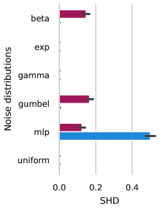
(a) Linear

(b) Nonlinear

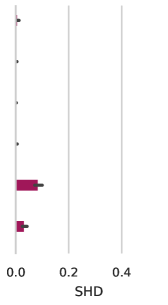
(c) PNL${}^{\textnormal{\ref{ft:pnl}}}$

Figure 1: In-distribution generalization of CSIvA trained and tested on data generated according to the same structural causal models, fixing mechanisms, and noise distributions between training and testing). As baselines for comparison, we use DirectLiNGAM on linear SCMs and NoGAM on nonlinear ANM (we use their causal-learn and dodiscover implementations). CSIvA performance is clearly non-trivial and generalizing well.

Out-of-distribution generalization.

In practice, we generally do not know the SCM defining the test distribution, so we are interested in CSIvA’s ability to generalize to data sampled from a class of causal models that is unobserved during training. We call this out-of-distribution generalization (OOD). We study OOD generalization to different noise terms, analyzing the network performance on datasets generated from causal models where the mechanisms are fixed with respect to the training, while the noise distribution varies (e.g., given linear-mlp training samples, testing occurs on linear-uniform data). Orthogonally to these experiments, we empirically validate CSIvA’s OOD generalization over different mechanism types (linear, nonlinear, post-nonlinear), while leaving the noise distribution (mlp) fixed across test and training. In Figure 2(a), we observe that CSIvA cannot generalize across the different mechanisms, as the SHD of a network tested on unseen causal mechanisms approximates that of the random baseline. Further, Figure 2(b) shows that out-of-distribution generalization across noise terms does not work reliably, and it is hard to predict when it might occur.

Implications.

CSIvA generalizes well to test data generated by the same class of SCMs used for training, in line with the findings in Ke et al. [1], which validates our implementation and training procedure. However, it struggles when the test data are out-of-distribution, not generated by causal models with the same mechanisms and noise terms it was trained on. While training on a wider class of SCMs might overcome this limitation, it requires caution. The identifiability of causal graphs indeed results from the interplay between the data-generating mechanisms and noise distribution. However, as we argue in our Example 1, the class of causal models that a supervised learning algorithm can identify is generally not clear. In what follows, we investigate this point and its implications for CSIvA, showing that the identifiability of the test samples can be ensured by imposing suitable assumptions on the class of SCMs generating the training distribution.

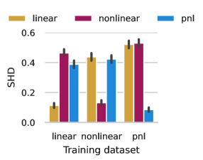
(a) Mechanisms

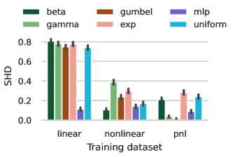
(b) Noise distributions

Figure 2: Out-of-distribution generalisation. We train three CSIvA models on data sampled from SCMs with linear, nonlinear additive, and post-nonlinear mechanisms; and noise fixed mlp noise distribution. In Figure (a) we test across different noise distributions, with test mechanisms fixed from training. In Figure (b) we test each network on different mechanisms and fixed mlp noise. CSIvA struggles to generalize to unseen causal mechanisms and often displays degraded performance over new noise distributions.

3.3 How does CSIvA relate to identifiability theory for causal graphs?

The CSIvA algorithm does not make structural assumptions about the causal model underlying the input data. This implies that the output of this method is unclear: as CSIvA targets the conditional distribution $p(\cdot|\mathcal{D})$ over the space of graphs, in the absence of restrictions on the functional mechanisms and the distribution of the noise terms, the causal graph $X\to Y$ is indistinguishable from $Y\to X$, as they are both equally likely to underlie the joint density $p_{X,Y}$ generating the data. As we discuss in Example 1, the graphical output of the trained architecture could at most identify the equivalence class of the true causal graph. Yet, our experiments of Section 3.2 show that CSIvA is capable of good in-distribution generalization, often inferring the correct DAG at test time. We explain this seeming contradiction with the following hypothesis, which motivates the analysis in the remainder of this section.

Hypothesis 1.

The class of structural causal models that can be identified by CSIvA is defined by the class of structural causal models underlying the generation of the training data.

To support and clarify our statement, we present the following example, adapted from Hoyer et al. [7].

Example 2.

Consider the causal model $Y=f(X)+N,$ where $f(X)=-X$ and $p_{X},p_{N}$ are Gumbel densities $p_{X}(x)=\operatorname{exp}(-x-\operatorname{exp}(-x))$ and $p_{N}(n)=\operatorname{exp}(-n-\operatorname{exp}(-n))$. This model satisfies the assumptions of the LiNGAM, so it is identifiable, in the sense that a backward linear model with the same distribution does not exist. However, in this special case, we can build a backward nonlinear additive noise model $X=g(Y)+\tilde{N}$ with independent noise terms: taking $p_{Y}(y)=\operatorname{exp}(-y-2\log(1+\operatorname{exp}(-y)))$ to be the density of a logistic distribution, $p_{\tilde{N}}(\tilde{n})=\operatorname{exp}(-2\tilde{n}-\operatorname{exp}(-\tilde{n}))$ and $g(y)=\log(1+\operatorname{exp}(-y))$; we see that $p_{X,Y}$ can factorize according to two opposite causal directions, as $p_{X,Y}(x,y)=p_{N}(y-f(x))p_{X}(x)=p_{\tilde{N}}(x-g(y))p_{Y}(y)$. Given a dataset $\mathcal{D}$ of observations from the forward linear model, causal discovery methods like DirectLiNGAM [34] can provably identify the correct causal direction $X\rightarrow Y$, assuming that sufficient samples are provided. Instead, the behavior of CSIvA seems hard to predict: given that the network approximates the conditional distribution $p(\cdot|\mathcal{D})$ over the possible graphs, for $\mathcal{D}$ with arbitrary many samples we have $p(X\rightarrow Y|\mathcal{D})=p(Y\rightarrow X|\mathcal{D})=0.5$. On the other hand, given the prior knowledge that the data-generating SCM is a linear non-gaussian additive noise model, we have $p(X\rightarrow Y|\mathcal{D},\textnormal{LiNGAM})=1$, because the LiNGAM is identifiable. In this sense, the class of structural causal models that CSIvA correctly infers appears to be determined by the structural causal models underlying the generation of the training data. Under our Hypothesis 1, training CSIvA exclusively on LiNGAM-generated data is equivalent to learning the distribution $p(\cdot|\mathcal{D},\textnormal{LiNGAM})$, such that the network should be able to identify the forward linear model, whereas it could only infer the equivalence class of the causal graph if its training datasets include observations from a nonlinear additive noise model.

The empirical results of Figure 3(a) show that CSIvA behaves according to our hypothesis: when training exclusively occurs on datasets $\{\mathcal{D}_{i,\to}\}_{i}$ generated by the forward linear-gumbel model of Example 2, the network can identify the causal direction of test data generated according to the same SCM. Similarly, the transformer trained on datasets $\{\mathcal{D}_{i,\leftarrow}\}_{i}$ from the backward nonlinear model of the example can generalize to test data coming from the same distribution. According to our claim, instead, the network that is trained on the union of the training samples $\{\mathcal{D}_{i,\to}\}_{i}\cup\{\mathcal{D}_{i,\leftarrow}\}_{i}$ from the forward and backward models (50:50 ratio in Figure 3(a)) displays the same test SHD (around $0.5$) as a random classifier assigning the causal direction with equal probability.

Further, we investigate CSIvA’s relation with known identifiability theory by training and testing the architecture on data from a linear Gaussian model, which is well-known to be unidentifiable. Not surprisingly, the results of Figure 3(b) show that none of the algorithms that we learn can infer the causal order of linear Gaussian models with test SHD any better than a random baseline.

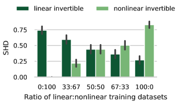
(a) Invertible data

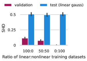
(b) Linear Gaussian test data

Figure 3: Experiments on identifiability theory. In Figure (a) we test the performance on linear-Gaussian data. Models are trained with different ratios of samples from linear and nonlinear SCMs with Gaussian noise terms. The validation results showcase that the networks were trained successfully. Figure (b) shows the SHD of models trained on different ratios of linear and nonlinear invertible data of Example 2. CSIvA behaves according to identifiability theory, failing to predict on linear Gaussian models and invertible data (50:50 ratio).

Implications.

Our experiments show that CSIvA learns algorithms that closely follow identifiability theory for causal discovery. In particular, while the method itself does not require explicit assumptions on the data-generating process, the chosen training data ultimately determines the class of causal models identifiable during inference. Notably, previous work has argued that supervised learning approaches in causal discovery would help with "dealing with complex data-generating processes and greatly reduce the need of explicitly crafting identifiability conditions a-priori", Lopez-Paz et al. [10]. In the case of CSIvA, this expectation does not appear to be fulfilled, as the assumptions still need to be encoded explicitly in the training data. However, this observation opens two new important questions: (1) Can we train a single network to encompass multiple (or even all) identifiable causal structures? (2) How much ambiguity might exist between these identifiable models?

3.4 A low-dimensions argument in favor of learning from multiple causal models

Example 2 of the previous section shows that elements of distinct classes of identifiable structural causal models, such as LiNGAM and nonlinear ANM, may become non-identifiable when we consider their union. In this section, we show that in the class of post-additive noise models given by equation (2) (obtained as the union of the LiNGAM, the nonlinear ANM, and the post-nonlinear model), the set of distributions that is non-identifiable is negligible. Our proposition extends the results of Hoyer et al. [7], which are limited to the case of linear and nonlinear additive noise models, and Zhang and Hyvärinen [8], which provides the conditions of identifiability of the post-ANM without bounding the set of non-identifiable distributions.

Let $X,Y$ be a pair of random variables generated according to the causal direction $X\rightarrow Y$ and the post-additive noise model structural equation:

$$Y=f_{2}(f_{1}(X)+N_{Y}),$$ (5)

where $N_{Y}$ and $X$ are independent random variables, and $f_{2}$ is invertible. If the SCM is non-identifiable, the data-generating process can be described by a backward model with the structural equation:

$$X=g_{2}(g_{1}(Y)+N_{X}),$$ (6)

$N_{X}$ independent from $Y$, and $g_{2}$ invertible. We introduce the random variables $\tilde{X},\tilde{Y}$, such that the forward and backward equations can be rewritten as

$$\begin{split}Y=f_{2}(\tilde{Y}),\hskip 10.00002pt\tilde{Y}\coloneqq f_{1}(X)+N_{Y},\\ X=g_{2}(\tilde{X}),\hskip 10.00002pt\tilde{X}\coloneqq g_{1}(Y)+N_{X}.\\ \end{split}$$

We note that this implies that the following invertible additive noise models on $\tilde{X},\tilde{Y}$ hold:

$$\tilde{Y}=h_{Y}(\tilde{X})+N_{Y},\hskip 10.00002pth_{Y}\coloneqq f_{1}\circ g_{2},$$ (7)

$$\tilde{X}=h_{X}(\tilde{Y})+N_{X},\hskip 10.00002pth_{X}\coloneqq g_{1}\circ f_{2}.$$ (8)

Proposition 1 (Adapted from Hoyer et al. [7]).

Let $p_{N_{Y}},h_{X},h_{Y}$ be fixed, and define $\nu_{Y}\coloneqq\log p_{N_{Y}}$, $\xi\coloneqq\log p_{\tilde{X}}$. Suppose that $p_{N_{Y}}$ and $p_{\tilde{X}}$ are strictly positive densities, and that $\nu_{Y},\xi,f_{1},f_{2},g_{1},$ and $g_{2}$ are three times differentiable. Further, assume that for a fixed pair $h_{Y},\nu_{Y}$ exists $\tilde{y}\in\mathbb{R}$ s.t. $\nu^{\prime\prime}_{Y}(\tilde{y}-h_{Y}(\tilde{x}))h^{\prime}_{Y}(\tilde{x})\neq 0$ is satisfied for all but a countable set of points $\tilde{x}\in\mathbb{R}$. Then, the set of all densities $p_{\tilde{X}}$ of $\tilde{X}$ such that both equations (5) and (6) are satisfied is contained in a 2-dimensional space.

Implications.

Our result is closely related to Theorem 1 of Hoyer et al. [7], which we simply generalize to the post-ANM. Intuitively, it says that the space of all continuous distributions such that the bivariate post-ANM is non-identifiable is contained in a 2-dimensional space. As the space of continuous distributions of random variables is infinite-dimensional, we conclude that the post-ANM is generally identifiable, which suggests that the setting of Example 2 is rather artificial. Our results provide a theoretical ground for training causal discovery algorithms on datasets generated from multiple identifiable SCMs. This is particularly appealing in the case of CSIvA, given the poor OOD generalization ability observed in our experiments of Section 3.2.

3.5 Can we train CSIvA on multiple causal models for better generalization?

In this section, we investigate the benefits of training over multiple causal models, i.e. on samples generated by a combination of classes of identifiable SCMs characterized by different mechanisms and noise terms distribution. Our motivation is as follows: given that our empirical evidence shows that CSIvA is capable of in-distribution generalization, whereas dramatically degrades the performance when testing occurs out-of-distribution, it is thus desirable to increase the class of causal models represented in the training datasets. We separately study the effects of training over multiple mechanisms and multiple noise distributions and compare the testing performance against architectures trained on samples of a single SCM.

(a) Linear test data

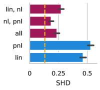
(b) Nonlinear test data

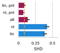
(c) PNL test data

Figure 4: Mixture of causal mechanisms. We train four models on samples from structural casual models with different mechanism types. We compare their test SHD (the lower, the better) against networks trained on datasets generated according to a single type of mechanism. The dashed line indicates the test SHD of a model trained on samples with the same mechanisms as test SCM. Training on multiple causal models with different mechanisms (mixed bars) always improves performance compared to training on single SCMs.

Mixture of causal mechanisms.

We consider four networks optimized by training of CSIvA on datasets generated from pairs (or triples) of distinct SCMs, with fixed mlp noise and which differ in terms of their mechanisms type: linear and nonlinear; nonlinear and post-nonlinear; linear and post-nonlinear; linear, nonlinear and post-nonlinear. The number of training datasets for each architecture is fixed ($15000$) and equally split between the causal models with different mechanism types. The results of Figure 4 show that the networks trained on mixtures of mechanisms all present significantly better test SHD compared to CSIvA models trained on a single mechanism type. We find that learning on multiple SCMs improves the SHD from $\sim 0.5$ to $\sim 0.2$ both on linear and nonlinear test data (Figures 4(a) and 4(b)), and even better accuracy is achieved on post-nonlinear samples, as shown in Figure 4(c).

Mixture of noise distributions.

Next, we analyze the test performance of three CSIvA networks optimized on samples from structural causal models that have different distributions for their noise terms, while keeping the mechanism types fixed. Figure 5 shows that training over different noises (beta, gamma, gumbel, exponential, mlp, uniform) always results in a network that is agnostic with respect to the noise distributions of the SCM generating the test samples, always achieving SHD $<0.1$, with the exception of datasets with mlp error terms ($0.2$ average SHD on nonlinear and pnl data).

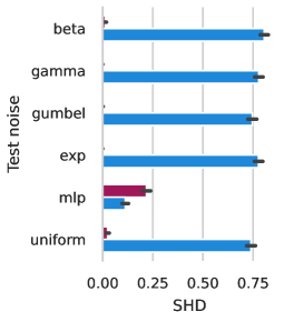
(a) Linear test data

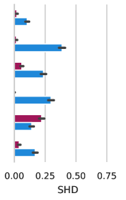
(b) Nonlinear test data

(c) PNL test data

Figure 5: Mixture of noise distributions. We train three networks on samples from SCMs with different noise terms distributions and fixed mechanism types: linear, nonlinear, and post-nonlinear. We present their test SHD (the lower, the better) on data from SCMs with the mechanisms fixed with respect to training, and noise terms changing between each dataset. Training on multiple causal models with different noises (all distributions bars) always improves performance compared to training on single SCMs with fixed mlp noise (only mlp bars).

Implications.

We have shown that learning on mixtures of SCMs with different noise term distributions and mechanism types leads to models generalizing to a much broader class of structural causal models during testing. Hence, combining datasets generated from multiple models looks like a promising framework to overcome the limited out-of-distribution generalization abilities of CSIvA observed in Section 3.2. However, it is easier to incorporate prior assumptions on the class of causal mechanisms (linear, non-linear, post-non-linear) compared to the noise distributions (which are potentially infinite). This introduces a trade-off between amortized inference and classical methods for causal discovery: for example, RESIT, NoGAM, and CAM [23, 35, 36] algorithms require no assumptions on the noise type, but only work for a limited class of mechanisms (nonlinear).

4 Conclusion

In this work, we investigate the interplay between identifiability theory and supervised learning for amortized inference of causal graphs, using CSIvA as the ground of our study. Consistent with classical algorithms, we demonstrate that good performance can be achieved if (i) we have a good prior on the structural causal model generating the test data (ii) the setting is identifiable. In particular, prior knowledge of the test distribution is encoded in the training data in the form of constraints on the structural causal model underlying their generation. With these results, we highlight the need for identifiability theory in modern learning-based approaches to causality, while past works have mostly disregarded this connection. Further, our findings provide the theoretical ground for training on observations sampled from multiple classes of identifiable SCMs, a strategy that improves test generalization to a broad class of causal models. Finally, we highlight an interesting new trade-off regarding identifiability: traditional methods like LiNGAM, RESIT, and PNL require strong restrictions on the structural mechanisms underlying the data generation (linear, nonlinear or post-nonlinear) while generally being agnostic relative to the noise terms distribution. Training on mixtures of causal models instead offers an alternative that is less reliant on assumptions on the mechanisms, while incorporating knowledge about all possible noise distributions in the training data is practically impossible to achieve. We leave it to future work to reproduce our analysis on a wider class of architectures, as well as extending our study to interventional data with more than two nodes.

Appendix A Learning to induce: causal discovery with transformers

A.1 A supervised learning approach to causal discovery

First, we describe the training procedure for the CSIvA architecture, which aims to learn the distribution of causal graphs conditioned on observational and/or interventional datasets. We omit interventional datasets from the discussion as they are not of interest to our work. Training data are generated from the joint distribution $p_{\mathcal{G},\mathcal{D}}$ between a graph $\mathcal{G}$ and a dataset $\mathcal{D}$. First, we sample a set of directed acyclic graphs $\{\mathcal{G}^{i}\}_{i=1}^{n}$ with nodes $X_{1},\ldots,X_{d}$, from a distribution $p_{\mathcal{G}}$. Then, for each graph we sample a dataset of $m$ observations of the graph nodes $\mathcal{D}^{i}=\{x_{1}^{j},\ldots,x_{d}^{j}\}_{j=1}^{m}$, $i=1,\ldots,n$. Hence, we build a training dataset $\{\mathcal{G}^{i},\mathcal{D}^{i}\}_{i=1}^{n}$.

The CSIvA model defines a distribution $\hat{p}_{\mathcal{G}|\mathcal{D}}(\cdot;\Theta)$ of graphs conditioned on the observational data and parametrized by $\Theta$. Given an invertible map $\mathcal{G}\mapsto A$ from a graph to its binary adjacency matrix representation of $d\times d$ entries (where $A_{ij}=1$ iff $X_{i}\rightarrow X_{j}$ in $\mathcal{G}$), we consider an equivalent estimated distribution $\hat{p}_{A|\mathcal{D}}(\cdot;\Theta)$, which has the following autoregressive form:

$$\hat{p}_{A,\mathcal{D}}(A|\mathcal{D};\Theta)=\prod_{l=1}^{d^{2}}\sigma(A_{l};\rho=f_{\Theta}(A_{1},\ldots,A_{l-1},\mathcal{D})),$$

where $\sigma(\cdot;\rho)$ is a Bernoulli distribution parametrized by $\rho$. $\rho$ itself is a function of $f_{\Theta}$ defined by the encoder-decoder transformer architecture, taking as input previous elements of the matrix $A$ (here represented as a vector of $d^{2}$ entries) and the dataset $\mathcal{D}$. $\Theta$ is optimized via maximum likelihood estimation, i.e. $\Theta^{*}=\operatorname*{argmin}_{\Theta}-\mathbf{E}_{\mathcal{G},\mathcal{D}}[\ln\hat{p}(\mathcal{G}|\mathcal{D};\Theta)]$, which corresponds to the usual cross-entropy loss for the Bernoulli distribution. Training is achieved using stochastic gradient descent, in which each gradient update is performed using a pair $(\mathcal{D}^{i},A^{i})$, $i=1\ldots,d$. In the infinite sample limit, we have $\hat{p}_{\mathcal{G}|\mathcal{D}}(\cdot;\Theta^{*})=p_{\mathcal{G}|\mathcal{D}}(\cdot)$, while in the finite-capacity case, it is only an approximation of the target distribution.

A.2 CSIvA architecture

In this section, we summarize the architecture of CSIvA, a transformer neural network that can learn a map from data to causally interpreted graphs, under supervised training.

Transformer neural network.

Transformers [25] are a popular neural network architecture for modeling structured, sequential data data. They consist of an encoder, a stack of layers that learns a representation of each element in the input sequence based on its relation with all the other sequence’s elements, through the mechanism of self-attention, and a decoder, which maps the learned representation to the target of interest. Note that data for causal discovery are not sequential in their nature, which motivates the adaptations introduced by Ke et al. [1] in their CSIvA architecture.

CSIvA embeddings.

Each element $x_{i}^{j}$ of an input dataset is embedded into a vector of dimensionality $E$. Half of this vector is allocated to embed the value $x_{i}^{j}$ itself, while the other half is allocated to embed the unique identity for the node $X_{i}$. We use a node-specific embedding because the values of each node may have very different interpretations and meanings. The node identity embedding is obtained using a standard 1D transformer positional embedding over node indices. The value embedding is obtained by passing $x_{i}^{j}$, through a multi-layer perceptron (MLP).

CSIvA alternating attention.

Similarly to the transformer’s encoder, CSIvA stacks a number of identical layers, performing self-attention followed by a nonlinear mapping, most commonly an MLP layer. The main difference relative to the standard encoder is in the implementation of the self-attention layer: as transformers are in their nature suitable for the representation of sequences, given an input sample of $D$ elements, self-attention is usually run across all elements of the sequence. However, data for causal discovery are tabular, rather than sequential: one option would be to unravel the $n\times d$ matrix of the data, where $n$ is the number of observations and $d$ the number of variables, into a vector of $n\cdot d$ elements, and let this be the input sequence of the encoder. CSIvA adopts a different strategy: the self-attention in each encoder layer consists of alternate passes over the attribute and the sample dimensions, known as alternating attention [37]. As a clarifying example, consider a dataset $\{(x_{1}^{i},x_{2}^{i})\}_{i=1}^{n}$ of $n$ i.i.d. samples from the joint distribution of the pair of random variables $X_{1},X_{2}$. For each layer of the encoder, in the first step (known as attention between attributes), attention operates across all nodes of a single sample $(x_{1}^{i},x_{2}^{i})$ to encode the relationships between the two nodes. In the second step (attention between samples), attention operates across all samples $(x_{k}^{1},\ldots,x_{k}^{n}),k\in\{1,2\}$ of a given node, to encode information about the distribution of single node values.

CSIvA encoder summary.

The encoder produces a summary vector $s_{i}$ with $H$ elements for each node $X_{i}$, which captures essential information about the node’s behavior and its interactions with other nodes. The summary representation is formed independently for each node and involves combining information across the $n$ samples. This is achieved with a method often used with transformers that involves a weighted average based on how informative each sample is. The weighting is obtained using the embeddings of a summary "sample" $n+1$ to form queries, and embeddings of node’s samples $\{x_{i}^{j}\}_{j=1}^{n}$ to provide keys and values, and then using standard key-value attention.

CSIvA decoder.

The decoder uses the summary information from the encoder to generate a prediction of the adjacency matrix $A$ of the underlying $\mathcal{G}$. It operates sequentially, at each step producing a binary output indicating the prediction $\hat{A}_{i,j}$ of $A_{i,j}$, proceeding row by row. The decoder is an autoregressive transformer, meaning that each prediction $\hat{A}_{i,j}$ is obtained based on all elements of $A$ previously predicted, as well as the summary produced by the encoder. The method does not enforce acyclicity, although Ke et al. [1] shows that in cyclic outputs genereally don’t occur, in practice.

Appendix B Training details

B.1 Hyperparameters

In Table 1 we detail the hyperparameters of the training of the network of the experiments. We define an iteration as a gradient update over a batch of $5$ datasets. Models are trained until convergence, using a patience of $5$ (training until five consecutive epochs without improvement) on the validation loss - this always occurs before the $25$-th epoch (corresponding to $\approx 150000$ iterations). The batch size is limited to $5$ due to memory constraints.

Hypeparameter	Value
Hidden state dimension	64
Encoder transformer layers	8
Decoder transformer layers	8
Num. attention heads	8
Optimizer	Adam
Learning rate	$10^{-4}$
Samples per dataset ($n$)	$1500$
Num. training datasets	$15000$
Num. iterations	$<150000$
Batch size	$5$

Table 1: Hyperparameters for the training of the CSIvA models of the experiments in Section 3.

B.2 Synthetic data

In this section, we provide additional details on the synthetic data generation, which was performed with the causally Python library [9]. Our data-generating framework follows that of Montagna et al. [9], an extensive benchmark of causal discovery methods on different classes of SCMs.

Causal mechanisms.

The nonlinear mechanisms of the PNL model and the nonlinear ANM model are generated by a neural network with one hidden layer with $10$ hidden units, with a parametric ReLU activation function. The network weights are randomly sampled according to a standard Gaussian distribution. The linear mechanisms are generated by sampling the regression coefficients in the range $[-3,-0.5]\cup[0.5,3]$.

Distribution of the noise terms.

We generated datasets from structural causal models with the following distribution of the noise terms: Beta, Gamma, Gaussian (for nonlinear data), Gumbel, Exponential, and Uniform. Additionally, we define the mlp distribution by nonlinear transformations of gaussian samples from a guassian distribution centered at zero and with standard deviation $\sigma$ uniformly sampled between $0.5$ and $1$. The nonlinear transformation is parametrized by a neural network with one hidden layer with $100$ units, and sigmoid activation function. The weights of the network are uniformly sampled in the range $[-1.5,1.5]$. We additionally standardized the output of each mlp sample by the empirical variance computed over all samples.

Data are standardized with their empirical variance, which removes the presence of shortcuts which could be learned by the network, notably varsortability [32] and score-sortability [33].

B.3 Computer resources

Our experiments were run on a local computing cluster, using any and all available GPUs (all NVIDIA). For replication purposes, GTX 1080 Ti’s are entirely suitable, as the batch size was set to match their memory capacity, when working with bivariate graphs. All jobs ran with $10\mathrm{GB}$ of RAM and $4$ CPU cores. The results presented in this paper were produced after $145$ days of GPU time, of which $68$ were on GTX 1080 Ti’s, $13$ on RTX 2080 Ti’s, $11$ on A10s, $19$ on A40s, and $35$ on RTX 3090s. Together with previous experiments, while developing our code and experimental design, we used 376 days of GPU time (for reference, at a total cost of $492.14$ Euros), similarly split across whichever GPUs were available at the time: $219$ on GTX 1080 Ti’s, $38$ on RTX 2080 Ti’s, $18$ on A10s, $63$ on RTX 3090s, $31$ on A40s, and $6$ on A100s.

Appendix C Further experiments

We present our experimental results on one further question, to help clarify the results in the main text of the paper. Our aim is to understand when to make tradeoffs between computational resources, and having models that have been trained on a wider variety of SCMs. We compare training on multiple SCMs to single-SCM training, when all models see the same amount of training data from each SCM type as a non-mixed model (i.e. a mixed network trains on $15,000$ linear datasets and $15,000$ PNL datasets, instead of $15,000$ divided between the two SCM types).

In the main text of this paper, we compare neural networks trained on a mix of structural causal models (e.g. noise distributions, or mechanism types), to models trained on a single mechanism-noise combination, where all models have the same amount of training data, $15,000$ datasets. In mixed training, we split these evenly, so a "lin, nl" model is trained on $7,500$ datasets from linear SCMs, and $7,500$ from nonlinear SCMs. Our results in this framework are promising, and show that for many combinations of SCM types, we can train one model instead of two, and achieve good progress, while making a $50\%$ savings on training costs. However, if our training budget is high/unlimited, we should also ask whether there is a downside to mixed training - can we achieve the same performance as a model trained on a single SCM type? Fig. 6 shows good results in this direction - the models trained with the same number of datasets per SCM type as an unmixed model had similar (or even better, for PNL data) performance as the un-mixed model trained on the same SCM type as the test data. These mixed models are also significantly more useful than having 2 or 3 separate models per SCM type, as they have good across-the-board performance. However, if we used the same computational resources to train 3 separate networks (one for each mechanism type) and wanted to use them for causal discovery on a dataset with unknown assumptions, we would be left with the rather difficult task of deciding which model to trust.

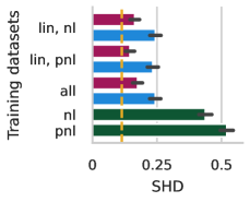
(a) Linear test data

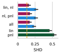
(b) Nonlinear test data

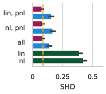
(c) PNL test data

Figure 6: Mixtures of causal mechanisms, with varying amounts of training data. We train eight models on samples from structural casual models with different mechanisms. Four (in purple), were trained on $15,000$ samples for each SCM type (so the "lin,nl" model saw $30,000$ samples in total, and the "all" model saw $45,000$), and the other four (blue) are the same as in Fig. 4, and were trained on $15,000$ samples in total, evenly split between the SCM types they were trained on. We compare their test SHD (the lower, the better) against networks trained on datasets generated according to a single type of mechanism. The dashed line indicates the test SHD of a model trained on samples with the same mechanisms as the test SCM. Training on multiple causal models with different mechanisms (mixed bars) always improves performance compared to training on single SCMs.

Appendix D Theoretical results and proofs

Before stating the proof of Proposition 1, we show under which condition the pair of random variables $X,Y$ satisfies the forward and backward models of equations (5), (6): this is relevant for our discussion, as the proof of Proposition 1 consists of showing that this condition is almost never satisfied.

Notation.

We adopt the following notation: $\nu_{X}\coloneqq\log p_{N_{X}}$, $\nu_{Y}\coloneqq\log p_{N_{Y}}$, $\xi\coloneqq\log p_{\tilde{X}}$, $\eta\coloneqq\log p_{\tilde{Y}}$, and $\pi\coloneqq\log p_{\tilde{X},\tilde{Y}}$.

Theorem 1 (Theorem 1 of Zhang and Hyvärinen [8]).

Assume that $X,Y$ satisfies both causal relations of equations (5) and (6). Further, suppose that $p_{N_{Y}}$ and $p_{\tilde{X}}$ are positive densities on the support of $N_{Y}$ and $\tilde{X}$ respectively, and that $\nu_{Y},\xi,f_{1},f_{2},g_{1},$ and $g_{2}$ are third order differentiable. Then, for each pair $(\tilde{x},\tilde{y})$ satisfying $\nu^{\prime\prime}_{Y}(\tilde{y}-h_{Y}(\tilde{x}))h_{Y}(\tilde{x})\neq 0$, the following differential equation holds:

$$\xi^{\prime\prime\prime}=\xi^{\prime\prime}\left(\frac{h^{\prime\prime}_{Y}}{h^{\prime}_{Y}}-\frac{\nu^{\prime\prime\prime}_{Y}h^{\prime}_{Y}}{\nu^{\prime\prime}_{Y}}\right)+\frac{\nu^{\prime\prime\prime}_{Y}\nu^{\prime}_{Y}h^{\prime\prime}_{Y}h^{\prime}_{Y}}{\nu^{\prime\prime}_{Y}}-\frac{\nu^{\prime}_{Y}(h^{\prime\prime}_{Y})^{2}}{h^{\prime}_{Y}}-2\nu^{\prime\prime}_{Y}h^{\prime\prime}_{Y}h^{\prime}_{Y}+\nu^{\prime}_{Y}h^{\prime\prime\prime}_{Y},$$

and $h_{X}$ is constrained in the following way:

$$\frac{1}{h^{\prime}_{X}}=\frac{\xi^{\prime\prime}+\nu^{\prime\prime}_{Y}(h^{\prime}_{Y})^{2}-\nu^{\prime}_{Y}h^{\prime\prime}_{Y}}{\nu^{\prime\prime}_{Y}h^{\prime}_{Y}},$$ (9)

where the arguments of the functions have been left out for clarity.

Proof of Theorem 1.

We demonstrate separately the two statements of the theorem.

Part 1.

Given that equations (5) and (6) hold, this implies that the forward and backward models on $\tilde{X},\tilde{Y}$ of equations (7) and (8) are also valid, namely that:

$$\tilde{Y}=h_{Y}(\tilde{X})+N_{Y},$$

$$\tilde{X}=h_{X}(\tilde{Y})+N_{X}.$$

These are the structural equations of two causal models, associated with the forward $\tilde{X}\rightarrow\tilde{Y}$ and backward $\tilde{Y}\rightarrow\tilde{X}$ graphs, respectively. Applying the Markov factorization of the distribution according to the forward direction, we get:

$$p_{{\tilde{X},\tilde{Y}}}(\tilde{x},\tilde{y})=p_{{\tilde{Y}|\tilde{X}}}(\tilde{y}|\tilde{x})p_{{\tilde{X}}}(\tilde{x})=p_{{N_{Y}}}(\tilde{y}-h_{Y}(\tilde{x}))p_{{\tilde{X}}}(\tilde{x}),$$

which implies

$$\pi(\tilde{x},\tilde{y})=\nu_{Y}(\tilde{y}-h_{Y}(\tilde{x}))+\xi(\tilde{x}),$$ (10)

for any $\tilde{x},\tilde{y}$. Similarly, the Markov factorization on the backward model implies:

$$\pi(\tilde{x},\tilde{y})=\nu_{X}(\tilde{x}-h_{X}(\tilde{y}))+\eta(\tilde{y}).$$ (11)

From (11), we have that:

$$\frac{\partial^{2}}{\partial\tilde{x}^{2}}\pi(\tilde{x},\tilde{y})=\nu^{\prime\prime}_{X}(\tilde{x}-h_{X}(\tilde{y}))$$

$$\frac{\partial^{2}}{\partial\tilde{x}\partial\tilde{y}}\pi(\tilde{x},\tilde{y})=-\nu^{\prime\prime}_{X}(\tilde{x}-h_{X}(\tilde{y}))h^{\prime}_{X}(\tilde{y}),$$

which implies

$$\frac{\partial}{\partial\tilde{x}}\left(\frac{\frac{\partial^{2}}{\partial\tilde{x}^{2}}\pi(\tilde{x},\tilde{y})}{\frac{\partial^{2}}{\partial\tilde{x}\partial\tilde{y}}\pi(\tilde{x},\tilde{y})}\right)=0.$$ (12)

Computing the same set of partial derivatives from (10), we find:

$$\frac{\partial^{2}}{\partial\tilde{x}^{2}}\pi(\tilde{x},\tilde{y})=\nu^{\prime\prime}_{Y}(\tilde{y}-h_{Y}(\tilde{x}))(h^{\prime}_{Y}(\tilde{x}))^{2}-\nu^{\prime}_{Y}(\tilde{y}-h_{Y}(\tilde{x}))h^{\prime\prime}_{Y}(\tilde{x})+\xi^{\prime\prime}(\tilde{x})$$

$$\frac{\partial^{2}}{\partial\tilde{x}\partial\tilde{y}}\pi(\tilde{x},\tilde{y})=-\nu^{\prime\prime}_{Y}(\tilde{y}-h_{Y}(\tilde{x}))h^{\prime}_{Y}(\tilde{x}).$$

from which follows:

$$\begin{split}\frac{\partial}{\partial\tilde{x}}\left(\frac{\frac{\partial^{2}}{\partial\tilde{x}^{2}}\pi(\tilde{x},\tilde{y})}{\frac{\partial^{2}}{\partial\tilde{x}\partial\tilde{y}}\pi(\tilde{x},\tilde{y})}\right)&=-2h^{\prime\prime}_{Y}+\frac{\nu^{\prime}_{Y}h^{\prime\prime\prime}_{Y}}{\nu^{\prime\prime}_{Y}h^{\prime}_{Y}}-\frac{\xi^{\prime\prime\prime}}{\nu^{\prime\prime}_{Y}h^{\prime}_{Y}}+\frac{\nu^{\prime\prime\prime}_{Y}\nu^{\prime}_{Y}h^{\prime\prime}_{Y}}{(\nu^{\prime\prime}_{Y})^{2}}-\frac{\nu^{\prime}_{Y}(h^{\prime\prime}_{Y})^{2}}{\nu^{\prime\prime}_{Y}(h^{\prime}_{Y})^{2}}+\frac{\xi^{\prime\prime}\nu^{\prime\prime\prime}_{Y}h^{\prime\prime}_{Y}}{(\nu^{\prime\prime}_{Y})^{2}\nu^{\prime\prime}_{Y}(h^{\prime}_{Y})^{2}}\\ &=0.\end{split}$$

where we drop the input arguments for conciseness. The equality with $0$ is given by the equality with (12). Manipulating the above expression, the first claim follows.

Part 2.

Next, we prove the constraint derived on $h_{X}$. To do this, we exploit the fact that $\tilde{Y}$ is independent of $N_{X}$, which implies the following condition [38]:

$$\frac{\partial^{2}}{\partial\tilde{y}\partial n_{x}}\log p(\tilde{y},n_{x})=0,$$ (13)

for any $(\tilde{y},n_{x})$. According to equations (7), (8), we have that:

$$\tilde{Y}=h_{Y}(\tilde{X})+N_{Y},$$

$$N_{X}=\tilde{X}-h_{X}(\tilde{Y}),$$

such that we can define an invertible map $\Phi:(\tilde{y},n_{x})\mapsto(\tilde{x},n_{Y})$. It is easy to show that the Jacobian of the transformation has determinant $|J_{\Phi}|=1$, such that

$$p(\tilde{y},n_{Y})=p(\tilde{x},n_{Y}),$$

where $(\tilde{x},n_{Y})=\Phi^{-1}(\tilde{y},n_{X})$. Thus, being $\tilde{X},N_{Y}$ independent random variables, we have that:

$$\log p(\tilde{y},n_{X})=\log p(\tilde{x})+\log p(n_{Y})=\xi(\tilde{x})+\nu_{Y}(n_{Y}).$$

Given that $\tilde{X}=h_{X}(\tilde{Y})+N_{X}$, we have that

$$\frac{\partial^{2}}{\partial\tilde{y}\partial\tilde{n}_{X}}\log p(\tilde{x})=\xi^{\prime\prime}h^{\prime}_{X},$$

while $N_{Y}=\tilde{Y}-h_{Y}(\tilde{X})$ implies

$$\frac{\partial^{2}}{\partial\tilde{y}\partial\tilde{n}_{X}}\log p(n_{Y})=-\nu^{\prime\prime}_{Y}h^{\prime}_{Y}+\nu^{\prime\prime}_{Y}h^{\prime}_{X}(h^{\prime}_{Y})^{2}-\nu^{\prime}_{Y}h^{\prime}_{X}h^{\prime\prime}_{Y},$$

such that

$$\log p(\tilde{x},n_{Y})=\xi^{\prime\prime}h^{\prime}_{X}+-\nu^{\prime\prime}_{Y}h^{\prime}_{Y}+\nu^{\prime\prime}_{Y}h^{\prime}_{X}(h^{\prime}_{Y})^{2}-\nu^{\prime}_{Y}h^{\prime}_{X}h^{\prime\prime}_{Y},$$

which must be equal to zero, being equal to the LHS of (13). Thus, we conclude that

$$\frac{1}{h^{\prime}_{X}}=\frac{\xi^{\prime\prime}+\nu^{\prime\prime}_{Y}(h^{\prime}_{Y})^{2}-\nu^{\prime}_{Y}h^{\prime\prime}_{Y}}{\nu^{\prime\prime}_{Y}h^{\prime}_{Y}},$$

proving the claim. ∎

D.1 Proof of Proposition 1

Proof.

Under the hypothesis that equations (5), (6) hold, i.e. when the data generating process satisfy both a forward and a backward model, by Theorem 1 we have that:

$$\xi^{\prime\prime\prime}(\tilde{x})=\xi^{\prime\prime}(\tilde{x})G(\tilde{x},\tilde{y})+H(\tilde{x},\tilde{y}),$$ (14)

where

$$G(\tilde{x},\tilde{y})=\left(\frac{h^{\prime\prime}_{Y}}{h^{\prime}_{Y}}-\frac{\nu^{\prime\prime\prime}_{Y}h^{\prime}_{Y}}{\nu^{\prime\prime}_{Y}}\right),$$

$$H(\tilde{x},\tilde{y})=\frac{\nu^{\prime\prime\prime}_{Y}\nu^{\prime}_{Y}h^{\prime\prime}_{Y}h^{\prime}_{Y}}{\nu^{\prime\prime}_{Y}}-\frac{\nu^{\prime}_{Y}(h^{\prime\prime}_{Y})^{2}}{h^{\prime}_{Y}}-2\nu^{\prime\prime}_{Y}h^{\prime\prime}_{Y}h^{\prime}_{Y}+\nu^{\prime}_{Y}h^{\prime\prime\prime}_{Y}.$$

Define $z\coloneqq\xi^{\prime\prime\prime}$, such that the above equation can be written as $z^{\prime}(\tilde{x})=z(\tilde{x})G(\tilde{x},\tilde{y})+H(\tilde{x},\tilde{y})$. given that such function $z$ exists, it is given by:

$$z(\tilde{x})=z(\tilde{x}_{0})e^{\int_{\tilde{x}_{0}}^{\tilde{x}}G(t,y)dt}+\int_{\tilde{x}_{0}}^{\tilde{x}}e^{\int_{\hat{t}}^{\tilde{x}}G(t,y)dt}H(\hat{t},y)d\hat{t}.$$ (15)

Let $\tilde{y}$ such that $\nu^{\prime\prime}_{Y}(\tilde{y}-h_{Y}(\tilde{x}))h^{\prime}_{Y}(\tilde{x})\neq 0$ holds for all but countable values of $\tilde{x}$. Then, $z$ is determined by $z(\tilde{x}_{0})$, as we can extend equation (15) to all the remaining points. The set of all functions $\xi$ satisfying the differential equation (14) is a 3-dimensional affine space, as fixing $\xi(\tilde{x}_{0}),\xi^{\prime\prime}(\tilde{x}_{0}),\xi^{\prime\prime}(\tilde{x}_{0})$ for some point $\tilde{x}_{0}$ completely determines the solution $\xi$. Moreover, given $\nu_{Y},h_{X},h_{Y}$ fixed, $\xi^{\prime\prime}$ is specified by (9) of theorem 1, which implies:

$$\xi^{\prime\prime}=\frac{\nu^{\prime\prime}_{Y}h^{\prime}_{Y}}{h^{\prime}_{X}}+\nu^{\prime}_{Y}h^{\prime\prime}_{Y}-\nu^{\prime\prime}_{Y}(h^{\prime}_{Y})^{2},$$

which confines $\xi$ solutions of (14) to a 2-dimensional affine space. ∎

References

- Ke et al. [2022] Nan Rosemary Ke, Silvia Chiappa, Jane X. Wang, Jorg Bornschein, Anirudh Goyal, Melanie Rey, Theophane Weber, Matthew Botvinick, Michael Curtis Mozer, and Danilo Jimenez Rezende. Learning to Induce Causal Structure. In International Conference on Learning Representations, September 2022. URL https://openreview.net/forum?id=hp_RwhKDJ5.
- Peters et al. [2017] Jonas Peters, Dominik Janzing, and Bernhard Schölkopf. Elements of Causal Inference: Foundations and Learning Algorithms. Adaptive Computation and Machine Learning. The MIT Press, Cambridge, Mass, 2017. ISBN 978-0-262-03731-0.
- Pearl [2009] Judea Pearl. Causality. Cambridge University Press, Cambridge, 2nd edition, 2009.
- Spirtes [2010] Peter Spirtes. Introduction to causal inference. Journal of Machine Learning Research, 11(54):1643–1662, 2010. URL http://jmlr.org/papers/v11/spirtes10a.html.
- Glymour et al. [2019] Clark Glymour, Kun Zhang, and Peter Spirtes. Review of causal discovery methods based on graphical models. Frontiers in Genetics, 10, 2019. ISSN 1664-8021. doi: 10.3389/fgene.2019.00524. URL https://www.frontiersin.org/articles/10.3389/fgene.2019.00524.
- Shimizu et al. [2006] Shohei Shimizu, Patrik O. Hoyer, Aapo Hyvärinen, and Antti Kerminen. A linear non-gaussian acyclic model for causal discovery. Journal of Machine Learning Research, 7:2003–2030, dec 2006. ISSN 1532-4435.
- Hoyer et al. [2008] Patrik Hoyer, Dominik Janzing, Joris M Mooij, Jonas Peters, and Bernhard Schölkopf. Nonlinear causal discovery with additive noise models. In D. Koller, D. Schuurmans, Y. Bengio, and L. Bottou, editors, Advances in Neural Information Processing Systems, volume 21. Curran Associates, Inc., 2008. URL https://proceedings.neurips.cc/paper/2008/file/f7664060cc52bc6f3d620bcedc94a4b6-Paper.pdf.
- Zhang and Hyvärinen [2009] Kun Zhang and Aapo Hyvärinen. On the identifiability of the post-nonlinear causal model. In Proceedings of the Twenty-Fifth Conference on Uncertainty in Artificial Intelligence, UAI ’09, page 647–655, Arlington, Virginia, USA, 2009. AUAI Press. ISBN 9780974903958.
- Montagna et al. [2023a] Francesco Montagna, Atalanti Mastakouri, Elias Eulig, Nicoletta Noceti, Lorenzo Rosasco, Dominik Janzing, Bryon Aragam, and Francesco Locatello. Assumption violations in causal discovery and the robustness of score matching. In A. Oh, T. Neumann, A. Globerson, K. Saenko, M. Hardt, and S. Levine, editors, Advances in Neural Information Processing Systems, volume 36, pages 47339–47378. Curran Associates, Inc., 2023a. URL https://proceedings.neurips.cc/paper_files/paper/2023/file/93ed74938a54a73b5e4c52bbaf42ca8e-Paper-Conference.pdf.
- Lopez-Paz et al. [2015] David Lopez-Paz, Krikamol Muandet, Bernhard Schölkopf, and Ilya Tolstikhin. Towards a learning theory of cause-effect inference. In Proceedings of the 32nd International Conference on International Conference on Machine Learning - Volume 37, ICML’15, page 1452–1461. JMLR.org, 2015.
- Li et al. [2020] Hebi Li, Qi Xiao, and Jin Tian. Supervised Whole DAG Causal Discovery, June 2020.
- Lippe et al. [2022] Phillip Lippe, Taco Cohen, and Efstratios Gavves. Efficient neural causal discovery without acyclicity constraints. In International Conference on Learning Representations, 2022. URL https://openreview.net/forum?id=eYciPrLuUhG.
- Lorch et al. [2022] Lars Lorch, Scott Sussex, Jonas Rothfuss, Andreas Krause, and Bernhard Schölkopf. Amortized inference for causal structure learning. In Alice H. Oh, Alekh Agarwal, Danielle Belgrave, and Kyunghyun Cho, editors, Advances in Neural Information Processing Systems, 2022. URL https://openreview.net/forum?id=eV4JI-MMeX.
- Szabo et al. [2016] Zoltan Szabo, Bharath Sriperumbudur, Barnabas Poczos, and Arthur Gretton. Learning theory for distribution regression. Journal of Machine Learning Research, 17:1–40, 09 2016.
- Brouillard et al. [2020] Philippe Brouillard, Sébastien Lachapelle, Alexandre Lacoste, Simon Lacoste-Julien, and Alexandre Drouin. Differentiable causal discovery from interventional data. In H. Larochelle, M. Ranzato, R. Hadsell, M.F. Balcan, and H. Lin, editors, Advances in Neural Information Processing Systems, volume 33, pages 21865–21877. Curran Associates, Inc., 2020. URL https://proceedings.neurips.cc/paper_files/paper/2020/file/f8b7aa3a0d349d9562b424160ad18612-Paper.pdf.
- Ke et al. [2023] Nan Rosemary Ke, Olexa Bilaniuk, Anirudh Goyal, Stefan Bauer, Hugo Larochelle, Bernhard Schölkopf, Michael Curtis Mozer, Christopher Pal, and Yoshua Bengio. Neural causal structure discovery from interventions. Transactions on Machine Learning Research, 2023. ISSN 2835-8856. URL https://openreview.net/forum?id=rdHVPPVuXa. Expert Certification.
- Scherrer et al. [2022] Nino Scherrer, Olexa Bilaniuk, Yashas Annadani, Anirudh Goyal, Patrick Schwab, Bernhard Schölkopf, Michael C. Mozer, Yoshua Bengio, Stefan Bauer, and Nan Rosemary Ke. Learning neural causal models with active interventions, 2022.
- Lachapelle et al. [2020] Sébastien Lachapelle, Philippe Brouillard, Tristan Deleu, and Simon Lacoste-Julien. Gradient-based neural dag learning. In International Conference on Learning Representations, 2020. URL https://openreview.net/forum?id=rklbKA4YDS.
- Ng et al. [2020] Ignavier Ng, AmirEmad Ghassami, and Kun Zhang. On the role of sparsity and dag constraints for learning linear dags. In Proceedings of the 34th International Conference on Neural Information Processing Systems, NIPS ’20, Red Hook, NY, USA, 2020. Curran Associates Inc. ISBN 9781713829546.
- Zheng et al. [2018] Xun Zheng, Bryon Aragam, Pradeep Ravikumar, and Eric P. Xing. Dags with no tears: Continuous optimization for structure learning. In Neural Information Processing Systems, 2018. URL https://api.semanticscholar.org/CorpusID:53217974.
- Zhang et al. [2022] Zhen Zhang, Ignavier Ng, Dong Gong, Yuhang Liu, Ehsan M Abbasnejad, Mingming Gong, Kun Zhang, and Javen Qinfeng Shi. Truncated matrix power iteration for differentiable DAG learning. In Alice H. Oh, Alekh Agarwal, Danielle Belgrave, and Kyunghyun Cho, editors, Advances in Neural Information Processing Systems, 2022. URL https://openreview.net/forum?id=I4aSjFR7jOm.
- Bello et al. [2022] Kevin Bello, Bryon Aragam, and Pradeep Kumar Ravikumar. DAGMA: Learning DAGs via m-matrices and a log-determinant acyclicity characterization. In Alice H. Oh, Alekh Agarwal, Danielle Belgrave, and Kyunghyun Cho, editors, Advances in Neural Information Processing Systems, 2022. URL https://openreview.net/forum?id=8rZYMpFUgK.
- Peters et al. [2014] Jonas Peters, Joris M. Mooij, Dominik Janzing, and Bernhard Schölkopf. Causal discovery with continuous additive noise models. J. Mach. Learn. Res., 15(1):2009–2053, jan 2014. ISSN 1532-4435.
- Löwe et al. [2020] Sindy Löwe, David Madras, Richard S. Zemel, and Max Welling. Amortized causal discovery: Learning to infer causal graphs from time-series data. In CLEaR, 2020. URL https://api.semanticscholar.org/CorpusID:219955853.
- Vaswani et al. [2017] Ashish Vaswani, Noam Shazeer, Niki Parmar, Jakob Uszkoreit, Llion Jones, Aidan N Gomez, Łukasz Kaiser, and Illia Polosukhin. Attention is all you need. In I. Guyon, U. Von Luxburg, S. Bengio, H. Wallach, R. Fergus, S. Vishwanathan, and R. Garnett, editors, Advances in Neural Information Processing Systems, volume 30. Curran Associates, Inc., 2017. URL https://proceedings.neurips.cc/paper_files/paper/2017/file/3f5ee243547dee91fbd053c1c4a845aa-Paper.pdf.
- Jin et al. [2024] Zhijing Jin, Yuen Chen, Felix Leeb, Luigi Gresele, Ojasv Kamal, Zhiheng Lyu, Kevin Blin, Fernando Gonzalez Adauto, Max Kleiman-Weiner, Mrinmaya Sachan, et al. Cladder: A benchmark to assess causal reasoning capabilities of language models. Advances in Neural Information Processing Systems, 36, 2024.
- Zhang et al. [2024] Jiaqi Zhang, Joel Jennings, Agrin Hilmkil, Nick Pawlowski, Cheng Zhang, and Chao Ma. Towards causal foundation model: on duality between causal inference and attention, 2024.
- Scetbon et al. [2024] Meyer Scetbon, Joel Jennings, Agrin Hilmkil, Cheng Zhang, and Chao Ma. Fip: a fixed-point approach for causal generative modeling, 2024.
- Gupta et al. [2023] Shantanu Gupta, Cheng Zhang, and Agrin Hilmkil. Learned causal method prediction, 2023.
- Uhler et al. [2012] Caroline Uhler, G. Raskutti, Peter Bühlmann, and B. Yu. Geometry of the faithfulness assumption in causal inference. The Annals of Statistics, 41, 07 2012. doi: 10.1214/12-AOS1080.
- Geirhos et al. [2020] Robert Geirhos, Jörn-Henrik Jacobsen, Claudio Michaelis, Richard Zemel, Wieland Brendel, Matthias Bethge, and Felix Wichmann. Shortcut learning in deep neural networks. Nature Machine Intelligence, 2:665–673, 11 2020. doi: 10.1038/s42256-020-00257-z.
- Reisach et al. [2021] Alexander G. Reisach, Christof Seiler, and Sebastian Weichwald. Beware of the simulated dag! causal discovery benchmarks may be easy to game. In Neural Information Processing Systems, 2021. URL https://api.semanticscholar.org/CorpusID:239998404.
- Montagna et al. [2023b] Francesco Montagna, Nicoletta Noceti, Lorenzo Rosasco, and Francesco Locatello. Shortcuts for causal discovery of nonlinear models by score matching, 2023b.
- Shimizu et al. [2011] Shohei Shimizu, Takanori Inazumi, Yasuhiro Sogawa, Aapo Hyvarinen, Yoshinobu Kawahara, Takashi Washio, Patrik Hoyer, and Kenneth Bollen. DirectLiNGAM: A direct method for learning a linear non-gaussian structural equation model. Journal of Machine Learning Research, 12, 01 2011.
- Montagna et al. [2023c] Francesco Montagna, Nicoletta Noceti, Lorenzo Rosasco, Kun Zhang, and Francesco Locatello. Causal discovery with score matching on additive models with arbitrary noise. In 2nd Conference on Causal Learning and Reasoning, 2023c. URL https://openreview.net/forum?id=rVO0Bx90deu.
- Bühlmann et al. [2014] Peter Bühlmann, Jonas Peters, and Jan Ernest. CAM: Causal additive models, high-dimensional order search and penalized regression. The Annals of Statistics, 42(6), dec 2014. URL https://doi.org/10.1214%2F14-aos1260.
- Kossen et al. [2021] Jannik Kossen, Neil Band, Clare Lyle, Aidan Gomez, Tom Rainforth, and Yarin Gal. Self-attention between datapoints: Going beyond individual input-output pairs in deep learning. In A. Beygelzimer, Y. Dauphin, P. Liang, and J. Wortman Vaughan, editors, Advances in Neural Information Processing Systems, 2021. URL https://openreview.net/forum?id=wRXzOa2z5T.
- Lin [1997] Juan Lin. Factorizing multivariate function classes. In M. Jordan, M. Kearns, and S. Solla, editors, Advances in Neural Information Processing Systems, volume 10. MIT Press, 1997. URL https://proceedings.neurips.cc/paper_files/paper/1997/file/8fb21ee7a2207526da55a679f0332de2-Paper.pdf.