Cross Far- and Near-Field Channel Measurement and Modeling in Extremely Large-scale Antenna Array (ELAA) Systems
Abstract
Technologies like ultra-massive multiple-input-multiple-output (UM-MIMO) and reconfigurable intelligent surfaces (RISs) are of special interest to meet the key performance indicators of future wireless systems including ubiquitous connectivity and lightning-fast data rates. One of their common features, the extremely large-scale antenna array (ELAA) systems with hundreds or thousands of antennas, give rise to near-field (NF) propagation and bring new challenges to channel modeling and characterization. In this paper, a cross-field channel model for ELAA systems is proposed, which improves the statistical model in 3GPP TR 38.901 by refining the propagation path with its first and last bounces and differentiating the characterization of parameters like path loss, delay, and angles in near- and far-fields. A comprehensive analysis of cross-field boundaries and closed-form expressions of corresponding NF or FF parameters are provided. Furthermore, cross-field experiments carried out in a typical indoor scenario at 300 GHz verify the variation of MPC parameters across the antenna array, and demonstrate the distinction of channels between different antenna elements. Finally, detailed generation procedures of the cross-field channel model are provided, based on which simulations and analysis on NF probabilities and channel coefficients are conducted for , , , and uniform planar arrays at different frequency bands.
Index Terms:
6G and beyond, Extremely large-scale antenna array, Near field, Channel measurement, Channel modeling.I Introduction
In light of enormous spatial multiplexing and beamforming gain, ultra-massive multiple-input-multiple-output (UM-MIMO) and reconfigurable intelligent surfaces (RISs) are of special interests since they effectively increase the communication range and enhance the capacity to meet the key performance indicators of sixth generation (6G) communications [1, 2]. These technologies both feature extremely large-scale antenna array (ELAA) systems that are equipped with hundreds or thousands of antennas. For such a large aperture size, different from massive MIMO for fifth generation (5G) communications, new features like near-field (NF) propagation and spatial non-stationarity arise and bring new challenges to channel modeling and characterization [3, 4].
In wireless communications, the electromagnetic (EM) radiation field is divided into the far-field (FF) region and the radiative NF region111The near-field region is subdivided into reactive NF and radiative NF. Since EM waves in the reactive NF are induced fields and do not set off from the antenna, we only refer to the radiative NF in this article.. The basis of the near- and far-field (NF-FF) demarcation is various. In the FF region, the EM field is usually approximated by planar waves, whereas the planar wavefront model (PWM) may fail for wireless communication systems with ELAAs. Therefore, most boundaries are defined by the impact of PWM on channel characteristics such as amplitude and phase. For instance, the most classic NF-FF boundary, Rayleigh distance [5], is defined by the distance between transmitter (Tx) and receiver (Rx) beyond which the maximum phase error across the antenna aperture by using the PWM is less than . Furthermore, by considering different arrival angles across elements in the antenna array, the variation of the projected aperture is taken into account in NF-FF demarcation [6]. Besides, other criteria for NF-FF demarcation are based on the impact on beamforming [7, 8] or system performance such as channel capacity [6, 9].
Despite these researches on NF-FF demarcation, the effect of cross near- and far-fields has not been implemented in MIMO channel models with ELAA systems. In this paper, we adapt the cluster-based statistical channel model in 3GPP TR 38.901 [10] to cross-field characterization of MIMO channels. Specifically, as scatterers are likely to be located in near- or far-field of the antenna array at Tx or Rx, we divide EM wave propagation into three parts, separated by its first and last bounce. For the propagation from the Tx to the first bounce scatterer (FBS), and that from the last bounce scatterer (LBS) to the Rx, multi-path component (MPC) parameters including propagation time and departure/arrival angles are characterized in near- and far-fields, respectively.
Since far-field and near-field MPC parameters are generated separately, the NF-FF demarcation is first implemented by comparing the NF-FF boundary with the relative location of the scatterer to the antenna array. Specially, the NF-FF boundary is not shared by all MPC parameters. Instead, each parameter defines its own NF-FF boundary, on account of the effect of its approximation by PWM on channel coefficients.
The main contributions of this work are summarized as follows:
-
•
A cross far- and near-field channel model for ELAA systems is developed. Based on the refined model framework where the EM wave propagation is divided by FBS and LBS, we improve the cluster-based statistical channel model in 3GPP TR 38.901 by differentiating the characterization of parameters including path loss, propagation time and departure/arrival angles in FF and NF.
-
•
Confirmatory cross-field experiments are carried out in a typical indoor scenario at 300 GHz. Equipped with a displacement platform and a rotator, the sounding system supports angular-resolved measurement of a virtual planar array with sub-millimeter precision. The analysis of the measurement result verifies the variation of MPC parameters across the antenna array, and demonstrates the distinction of channels between different antenna elements in the scenario where scatterers are located in the cross-field of the array.
-
•
Detailed generation procedure of the cross-field channel model for ELAA systems is provided, based on the comprehensive analysis of cross-field boundaries and closed-form characterization of parameters. Channel simulations and analysis on NF probabilities and channel coefficients for , , , and uniform planar arrays (UPAs) at sub-6 GHz and mmWave frequency bands are then carried out in a UMa scenario.
The remainder of this paper is organized as follows. The cross-field MIMO channel model framework is first introduced in Section II, followed by the analysis of closed-form cross-field boundaries and characterization of parameters in Section III. In Section IV, a probative measurement with virtual uniform planar array at 300 GHz is carried out and the measurement results are discussed. We then elaborate the implementation of the cross-field MIMO channel model and the simulation result in Section V. Finally, the paper is concluded in Section VI.
II Cross-field Channel Model Framework
Before jumping into the analysis of NF-FF boundaries for each parameter, the channel model framework based on twin scatterers is first introduced. This starts with the notations in the single-input-single-output (SISO) channel model, which is then extended to the proposed MIMO channel model.
II-A Channel Model based on Twin Scatterers
A SISO channel model, simplified by omitting the change of channel coefficients caused by time variation and frequency offset of the subcarrier, is expressed as
| (1) |
where there are one line-of-sight (LoS) cluster () and non-line-of-sight (NLoS) clusters () from the transmitter (Tx) to the receiver (Rx).
Each NLoS cluster is related with a pair of scatterers, named by twin scatterers, i.e., one first-bounce scatterer (FBS) and one last-bounce scatterer (LBS). As a result, each NLoS path is divided into three parts, represented by the vector from Tx to FBS , the vector from FBS to LBS , and the vector from LBS to Rx . In the cluster, there are paths (e.g., for the LoS path, ). The delay of each path is denoted as , while indicates the azimuth angle of departure (AoD), zenith angle of departure (ZoD), azimuth angle of arrival (AoA) and zenith angle of arrival (ZoA) of the path. represents the path gain.
We first consider the cluster parameter. Due to the division of the propagation path, the delay of the cluster is also composed of three parts correspondingly, i.e., . The first part from Tx to FBS determines , as well as angles of departure and . where and denotes the speed of light. Take the position of Tx as the origin, the spherical coordinate (, , ) defines the position of FBS relative to Tx, which is equivalent to . For the second part, the virtual path between FBS and LBS, we only consider the influence of distance on the second term in the cluster delay by , while the direction is neglected. The third part from LBS to Rx determines , as well as angles of arrival and . where . The spherical coordinate (, , ) defines the position of LBS relative to Rx, which is equivalent to . The cluster gain is denoted as .
For each path in the cluster, the cluster power is equally divided, i,e, the path gain is for . The delay and angles of each path are generated based on the corresponding cluster parameter and intra-cluster spreads, by following the procedures in 3GPP TR 38.901.
II-B Multiple-Input-Multiple-Output Channel Model
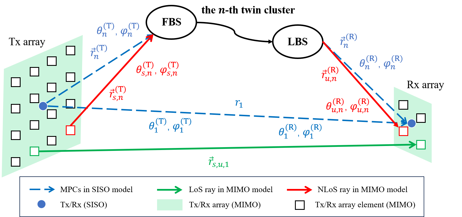
Before path generation inside each cluster, we need to consider different cluster parameters at each element. Therefore, we introduce the index for Tx element, , and the index for Rx element, . Then, we need to extend the clusters’ delay departure angle (, ), arrival angle (, ), gain , and number of path in the SISO model to cluster parameters at different antenna elements, , , , , , and .
| Symbol | Meaning |
| Index of cluster | |
| Index of path | |
| Index of antenna element at Tx | |
| Index of antenna element at Rx | |
| Carrier frequency | |
| Wavelength | |
| Ricean K-factor | |
| Time of arrival (delay) | |
| Power | |
| Zenith and azimuth angles | |
| Antenna pattern | |
| Cross-polarization power ratio | |
| Unit vector at the direction | |
| Motion of Rx |
Refer to the channel model for large antenna array in Section 7.6.2 of 3GPP TR 38.901, the general form of the cross-field MIMO channel model is composed of channel impulse responses of element-to-element links, as
| (2) | ||||
where
| (3) | ||||
and
| (4) | ||||
We apply the twin-scatterer-based framework and separate the propagation path into three parts. The first part goes from the element at Tx to the th FBS, which is characterized by distance , azimuth angle of departure and zenith angle of departure . The last part goes from the th LBS to the element at Rx, which is characterized by distance , azimuth angle of departure and zenith angle of departure . In the middle of the twin scatterer, the link from FBS to LBS is regarded as a virtual path, whose path length is fixed by . Therefore, the total time of arrival from the (, )th element at Tx to the element at Rx is , and the departure and arrival angles are indicated by .
II-C Cross-Field MIMO Channel Modeling
The major difference between NF and FF MIMO channel is the characterization of path parameters, which is array-level under FF assumption and element-level in the NF case. To model the parameters in the cross-field, the evaluation of parameters is different based on whether a scatterer is in the NF or FF region of an antenna array. The partition is based on the comparison of the NF/FF boundary and the distance between the scatter and the array center.
First, since the propagation path is divided into three parts by Tx, FBS, LBS and Rx, NF/FF regions are distinguished respectively for parameters between the FBS and Tx array (for instance , , ), and those between the LBS and the Rx array (for instance , , ).
Second, different parameters, i.e., path length and angles, do not share the same NF/FF boundary. Instead, the NF-FF boundary is specific for each parameter and its corresponding approximation method. In particular, for each approximation method of a parameter, we first calculate the magnitude/phase error between the approximation and the ground truth given by the spherical-wave model (SWM). Then, we derive the corresponding NF-FF boundary by limiting this error to the maximum tolerance of magnitude/phase error.
III Large- and Small-scale Parameters in Cross-Field
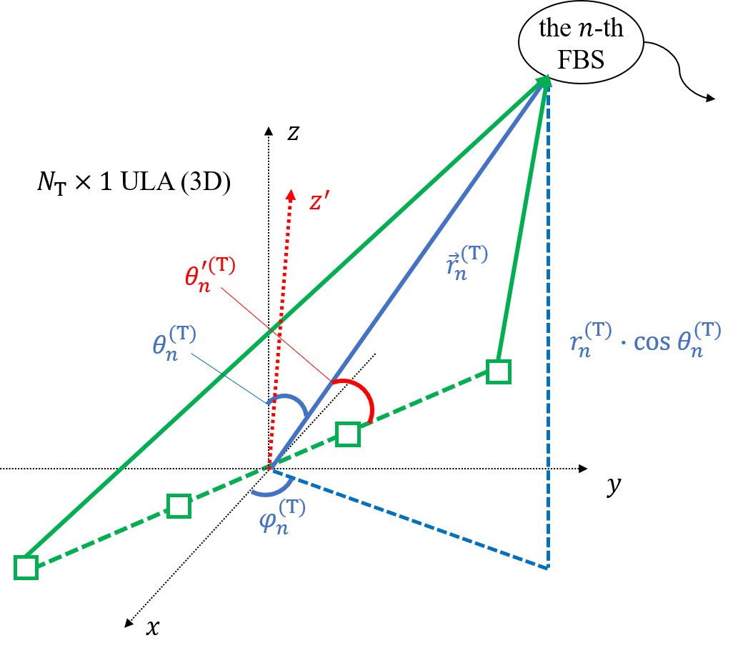
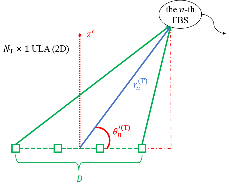
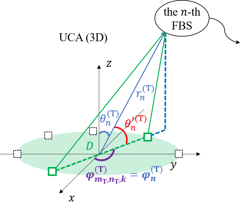
In this section, we determine the large- and small-scale parameters in the cross-field and derive respective NF-FF boundaries for each parameter. The following analysis is by default specific to parameters between FBS and a UPA at Tx, with element spacing . The index of antenna element can be equivalently replaced by (,). The analysis for other antenna array types, like uniform linear array (ULA) and uniform circular array (UCA) is also provided in this section. The analysis is similar for parameters between LBS and arrays at Rx.
III-A Delay in Cross-Field
The following discussion mainly focuses on the approximation of the propagation length from the (, )th element (, ) in Tx-UPA to the FBS, . The corersponding delay (or propagation time) can be derived by .
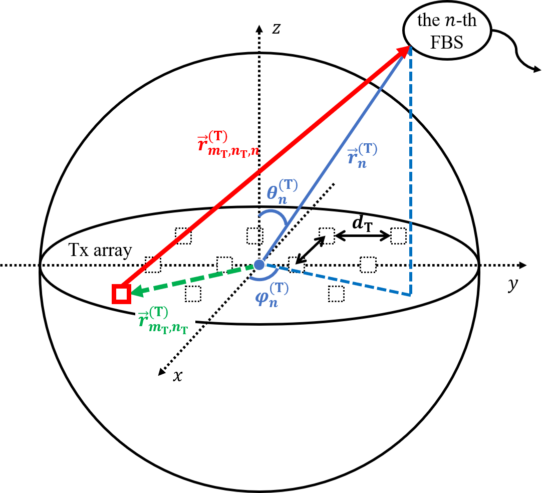
The vector from the Tx-UPA center to the FBS is represented by . In the local coordinate system shown in Fig. 2, where the UPA lies in the -plane and the center of UPA is the origin, (, , ) indicates the spherical coordinate of the FBS. Note that is the zenith angle rather than the elevation angle. Denote the vector as
| (5a) | ||||
| (5b) | ||||
where is a unit vector.
The vector from the Tx-UPA center to the (, )th antenna element is represented by . Since the element spacing is , the Cartesian coordinate of the element in the local coordinate system is (, , 0), where and . We denote the vector
| (6) |
The vector from the (, )th antenna element to the FBS is represented by , which can be derived by . Then the accurate distance between the (, )th antenna element and the th FBS is expressed as
| (7) | ||||
which is based on the spherical wave model. For a UPA with element spacing , the components in the formula can be specified as
| (8) | ||||
| (9) |
For a ULA along the -axis with element spacing , the components in the formula can be specified as
| (10) |
| (11) |
III-A1 Taylor approximation
By two-variable Taylor expansion in terms of (, ), the approximation can be derived as follows.
To start with, the Taylor approximation (planar wave assumption) is the first two terms of Taylor expansion, whose general form is
| (12) |
In this case, the deviation comes from the third term of the Taylor expansion, as
| (13) |
The Taylor approximation is the first three terms of Taylor expansion, whose general form is
| (14) |
In this case, the deviation comes from the fourth term of the Taylor expansion, as
| (15) |
Taking the ULA along -axis as example, by restricting the phase deviation to , the FF approximation is valid when
| (16) |
The FF approximation is valid when
| (17) |
where is the antenna array size. Among different pairs of angles, the worst case is
| (18) |
for the FF approximation and
| (19) |
for the FF approximation.
For the UPA case, . For the UCA case, is the diameter of the circle.
III-A2 Sub-array approximation
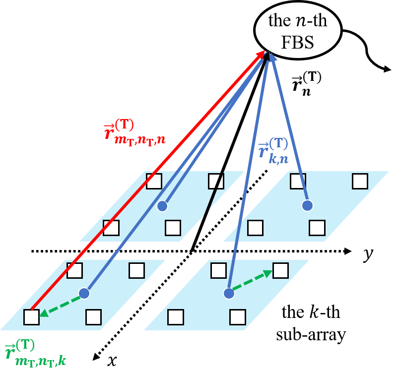
Aside from the Taylor approximation, another method is to divide the antenna array into sub-arrays, so that planar wave assumption is valid inside each sub-array [11, 8]. Specifically, first, the center of each sub-array is accurately determined by the geometric relation. Then, taking the sub-array center as the reference, the path length from the scatterer to elements in the sub-array is approximated by planar wave assumption. Detailed expressions are as follows. Assume and denote the number of sub-arrays in two directions, then each sub-array contains elements. First, for the th subarray (), the vector from the sub-array center to the FBS, , is accurately calculated. Then, for each element in the th sub-array, vector represents the position of the (, )th element relative to the Tx-UPA center. Finally, the Taylor approximation is used to calculate the distance between the (, )th element to the FBS.
III-A3 Evaluation and comparison
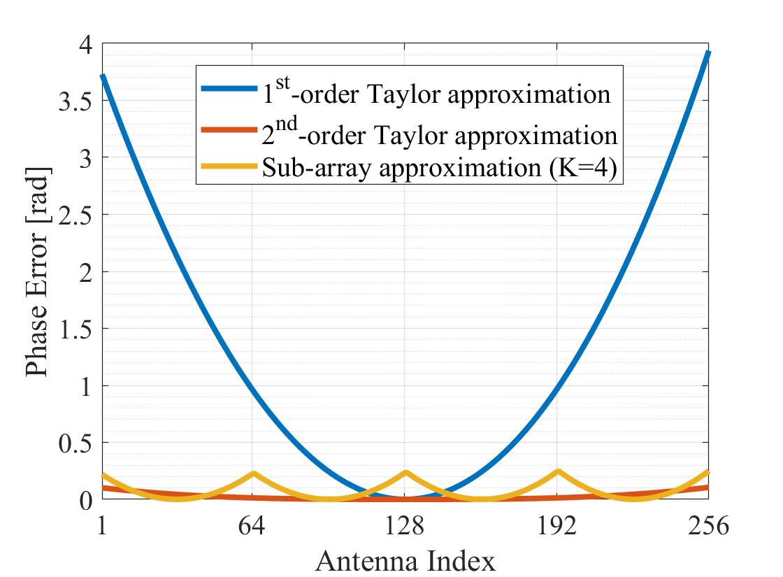
Take a ULA along -axis as an example, assume the carrier frequency is 100 GHz, the element spacing is half-wavelength, the number of elements is 256. The FBS position relative to Tx is defined by = (5 m, , ). Sub-array number is , with 64 elements in each sub-array. Under this setting,
-
•
The NF-FF boundary of the Taylor approximation (planar wave assumption), i.e., Rayleigh distance, is 97.5375 m.
-
•
The NF-FF boundary of the Taylor approximation, i.e., Fresnel distance, is 2.6778 m, which is far less than that of the Taylor approximation.
-
•
The NF-FF boundary of the Taylor approximation inside each sub-array is 5.9535 m, which is close to the distance from the scatterer to the array center 5 m.
Figure 4 shows the comparison of three approximation methods in terms of the phase error at each antenna element. Specifically, using the Taylor approximation (planar wave assumption), when the array expands to more than 56 elements, the phase error exceeds and degrades significantly. Using the sub-array division method, the change of phase error is the same inside each sub-array. However, since the center of each sub-array is accurate, and the division of sub-arrays guarantees the feasibility of planar wave assumption, the maximum phase error is always smaller than . In contrast, the increment of phase error is obviously slowed down using the Taylor approximation. In this example, the phase error exceeds when the number of antenna elements in a ULA reaches 386, which is superfluous in the practical case.
| Method | Taylor approximation | Sub-array division | ||||
| Prons | direct calculation, free of other steps |
|
||||
| bounded maximum path length (phase) error | ||||||
| Cons |
|
|
||||
|
||||||
| The Taylor approximation (planar wave assumption) is used inside each sub-array. | ||||||
III-B Zenith and Azimuth Angles in Cross-Field
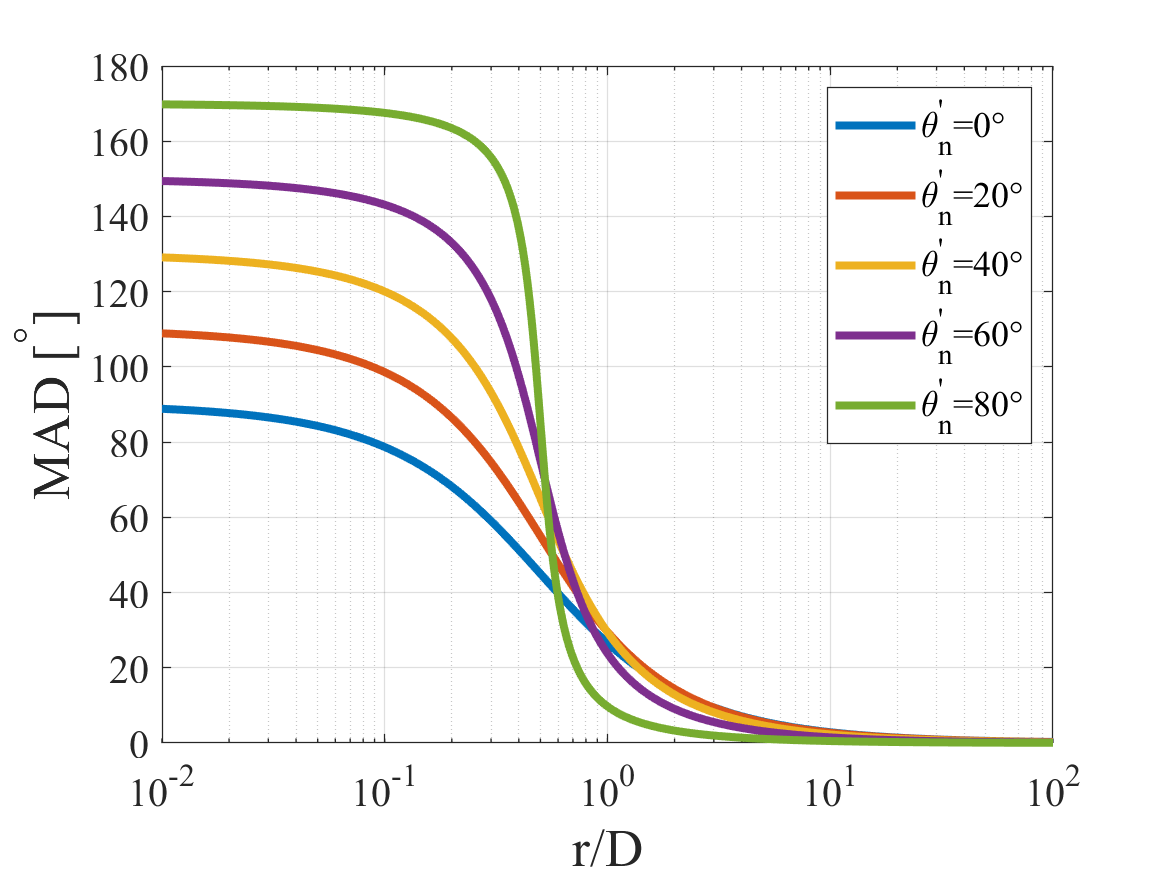
Given the antenna array size and the position of the scatterer (characterized by the distance between the scatterer and the array center , zenith angle , and azimuth angle ), we first explore how the actual angle at elements across the array differs from the angle at the array center. We define its maximum difference as the Maximum Angle Difference (MAD).
Similar to the definition of Rayleigh distance and Fresnel distance, which derive the NF-FF boundaries of path length by restricting the maximum phase difference to , we first obtain the express of MAD and then derive the NF-FF boundary of angles by restricting it to half of the half-power beamwidth (HPBW).
III-B1 Zenith angle in the ULA case
First, take the ULA along the -axis as the example, the expression of MAD is derived from the geometric relation, as
| (20) |
Note that since when , is an elevation angle with the range of . In contrast, in Fig. 5 is a zenith angle with the range of . In the same coordinate system, the sum of the elevation angle and the zenith angle is . However, in the ULA case, is not in the same coordinate system with and thus cannot be simply calculated by . Instead, is defined by the angle between the ULA and the vector .
When is fixed, MAD is monotonically decreasing with the ratio , as shown in Fig. 6.
By restricting
| (21) |
where is the vertical half-power beamwidth, we derive the lower bound of the distance between the scatterer and the array center (or the ratio ), as
| (22) |
which can be regarded as the NF-FF boundary of the zenith angle. If (22) is valid, we can assume that the zenith angle of the scatter at any antenna element is the same as the zenith angle at the array center, otherwise, the zenith angle should be accurately calculated.
III-B2 Zenith angle in UPA and UCA cases
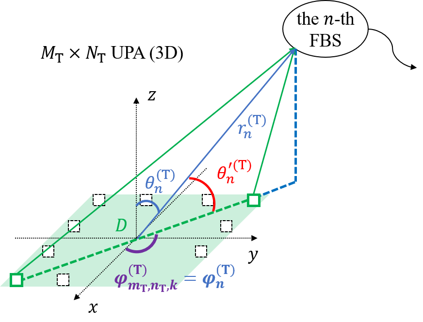
The aforementioned derivation is based on the ULA. In the case of UPA, as shown in Fig. 7(a), the worst case happens when the projection of coincides with the vector from the array center to the farest element, i.e.,
| (23) |
In this case, we can substitute
| (24) |
into the derivation in the ULA case and reuse (20) and (22). Still, note that the definition of is defined as the elevation angle under the local coordinate system that regards the UPA as the -plane (i.e., the normal vector of the UPA is the -axis), and thus can be derived by . If the UPA does not lie in the -plane, we need to calculate as minus the angle between and the normal vector of the UPA.
Similarly, in the case of UCA, as shown in Fig. 7(b), we can substitute
| (25) |
into (20) and (22), where is the radius of the UCA. Still, the definition of is defined as the elevation angle under the local coordinate system that regards the UCA as the -plane, i.e., the normal vector of the UCA is the -axis. If the UCA does not lie in the -plane, we need to calculate as minus the angle between and the normal vector of the UCA.
III-B3 Azimuth angle
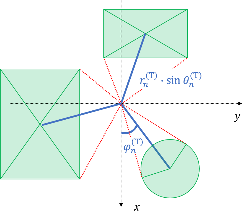
The aforementioned derivation is targeted at the zenith/elevation angle. For the azimuth angle, we can observe the projection of the scatterer on the -plane as shown in Fig. 7(c). The maximum azimuth angle difference occurs at four vertex of the UPA. Therefore, we can simply calculate the azimuth angle difference at these four positions and take their maximum, as
| (26) | ||||
In the case of UCA, as shown in Fig. 7(c), the maximum azimuth angle difference is half of the angle between two tangent lines of the UCA with radius , i.e., .
The value of MAD is then compared with half of the horizontal HPBW. If
| (27) |
we can assume that the azimuth angle of the scatterer at any antenna element is the same as that at the array cente. Otherwise, the azimuth angle should be accurately calculated.
III-C Path Gain in Cross-Field
While the antenna gain difference is larger than 3 dB across the array resulting from the deviation of incident angles that exceeds half of the half-power beamwidth (HPBW), another smaller-scale path gain deviation that should be involved in cross-field channel modeling is the gain reduction factor of the waveguides in the near-field [12, 13]. In specific, the free-space path loss of the vertically incident ray at each element can be statistically modeled by
| (28a) | |||
| (28b) | |||
where is the cross-field factor associated with the wavelength (or equivalently the frequency ), the distance from the scatter to the perpendicular array, and the coordinate of the element relative to the center (, ). The constant reference distance is a model parameter. In the proposed cross-field MIMO channel model, it can applied to the LoS ray when antenna arrays are face-to-face. Though, the significance of this gain variation is so far inconclusive, and more efforts are required to generalize the model to arbitrary postures of antenna arrays.
III-D Evaluation and Discussions
In the near-field channel modeling, for each parameter of the cluster, i.e., path length (or delay) and angles, we use the NF-FF boundary to determine whether the corresponding approximation method of the parameter is valid. The approximation of the parameter is valid in the FF field, otherwise, we require a more accurate calculation of the parameter. The following table summarizes the NF-FF boundaries corresponding to the approximation method of small-scale parameters.
| Parameter | FF approximation | Max deviation w.r.t array center | NF-FF boundary (BS-FBS as the example) |
| Path length | approx. (12) | in path length, or in phase | general: (16); worst: (18) |
| Path length | approx. (14) | in path length, or in phase | general: (17); worst: (19) |
| Zenith angle | same as that at array center | (22) | |
| Horizontal angle | same as that at array center | (27) |
Since antennas are usually/nearly omni-directional in the horizontal direction, we can assume the horizontal angle at each element remains the same as that at the array center.
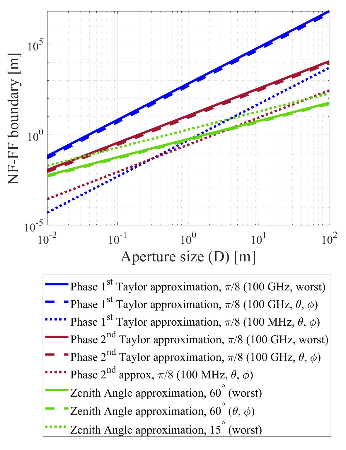
Take carrier frequency GHz, azimuth angle of departure , zenith angle of departure , max phase deviation , vertical HPBW at Tx (in other words, max zenith angle difference ) as the example, Fig. 8 compares the NF-FF boundaries, i.e., (16), (17), and (22), under different antenna array size .
Meanwhile, NF-FF boundaries in the worst case are also depicted in the same figure. The worst/largest NF-FF boundaries of path length, (18) and (19), are derived by traversing the value of angles (, ), while the worst/largest NF-FF boundary of zenith angle is derived by traversing the value of angles (, ) at . For arbitrary , the NF-FF boundary of the zenith angle becomes larger/worse when gets smaller.
As we can observe from the result,
-
•
NF-FF boundaries, in terms of distance between the scatterer and the array center ( or ), is proportional to the power of antenna array size . Specifically, the NF-FF boundary of the zenith angle is proportional to , the NF-FF boundary of path length using the Taylor approximation is proportional to , and the NF-FF boundary of path length using the Taylor approximation is proportional to . As a result, when the antenna array size grows, the FF approximation is more likely to fail for the path length with and then for the zenith angle.
-
•
The NF-FF boundaries of angles are independent of the carrier frequency (or wavelength), while the NF-FF boundaries of path length are relevant to the carrier frequency.
-
•
For the NF-FF boundary of path loss, at 100 GHz, the boundary at specific angles (blue/red long dashed lines) is close to the worst boundary (blue/red solid line). In contrast, the order of the carrier frequency directly affects the order of the boundary, which means the frequency is more influential to the boundary than the angles. For instance, when the frequency decreases from 100 GHz to 100 MHz, the order of the boundary decreases correspondingly (blue/red short dashed line).
-
•
For the NF-FF boundary of angles, at 100 GHz, the boundary at specific angles (green long dashed lines) is close to the worst boundary (green solid line). The boundary does not change with frequency. However, the value of the HPBW is more influential to the boundary than the value of angles (green short dashed line).
IV Cross-Field Channel Measurement and Result
In this section, we describe the measurement conducted in the cross near- and far-field scenario.
IV-A Channel Measurement System
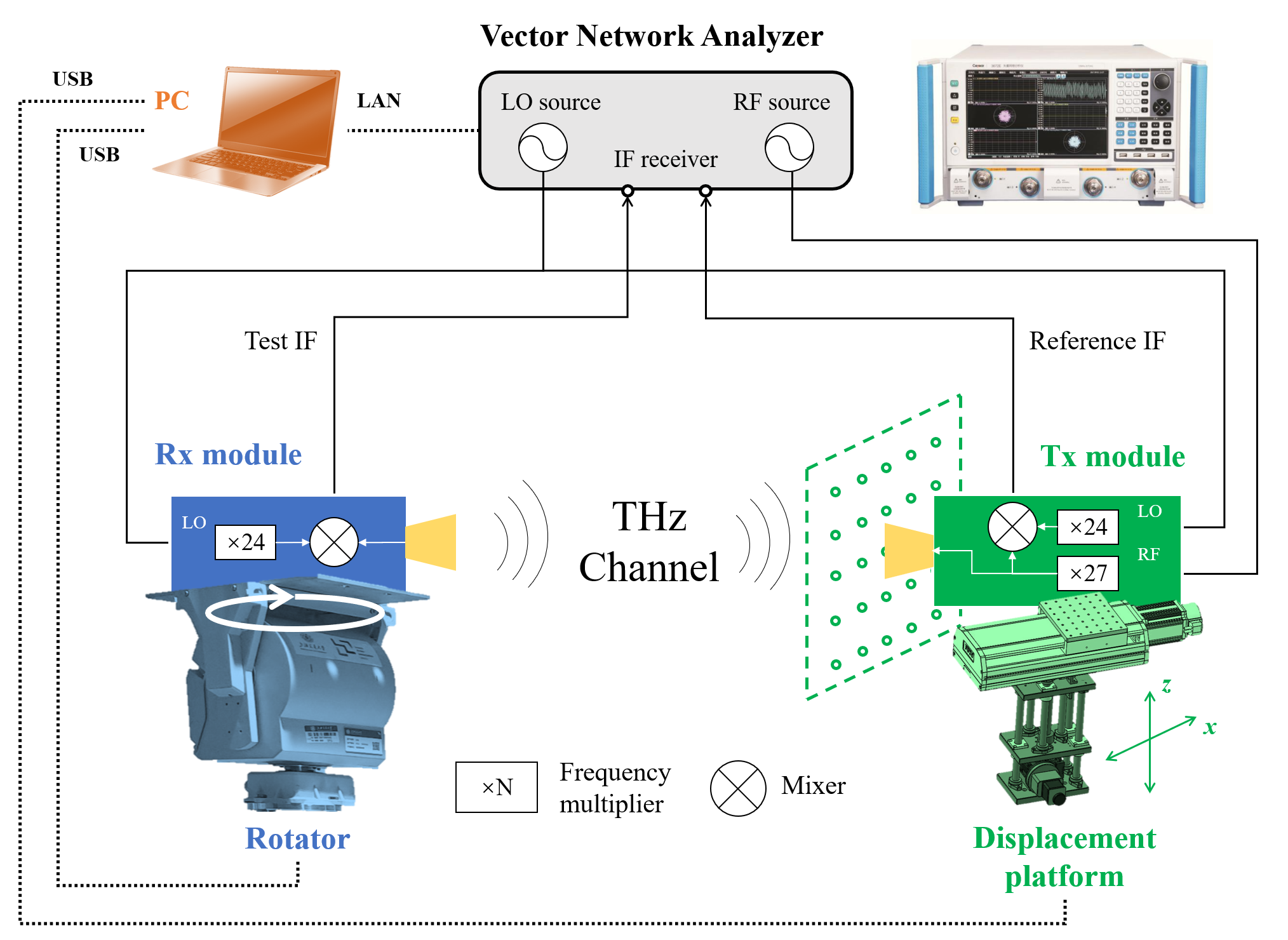
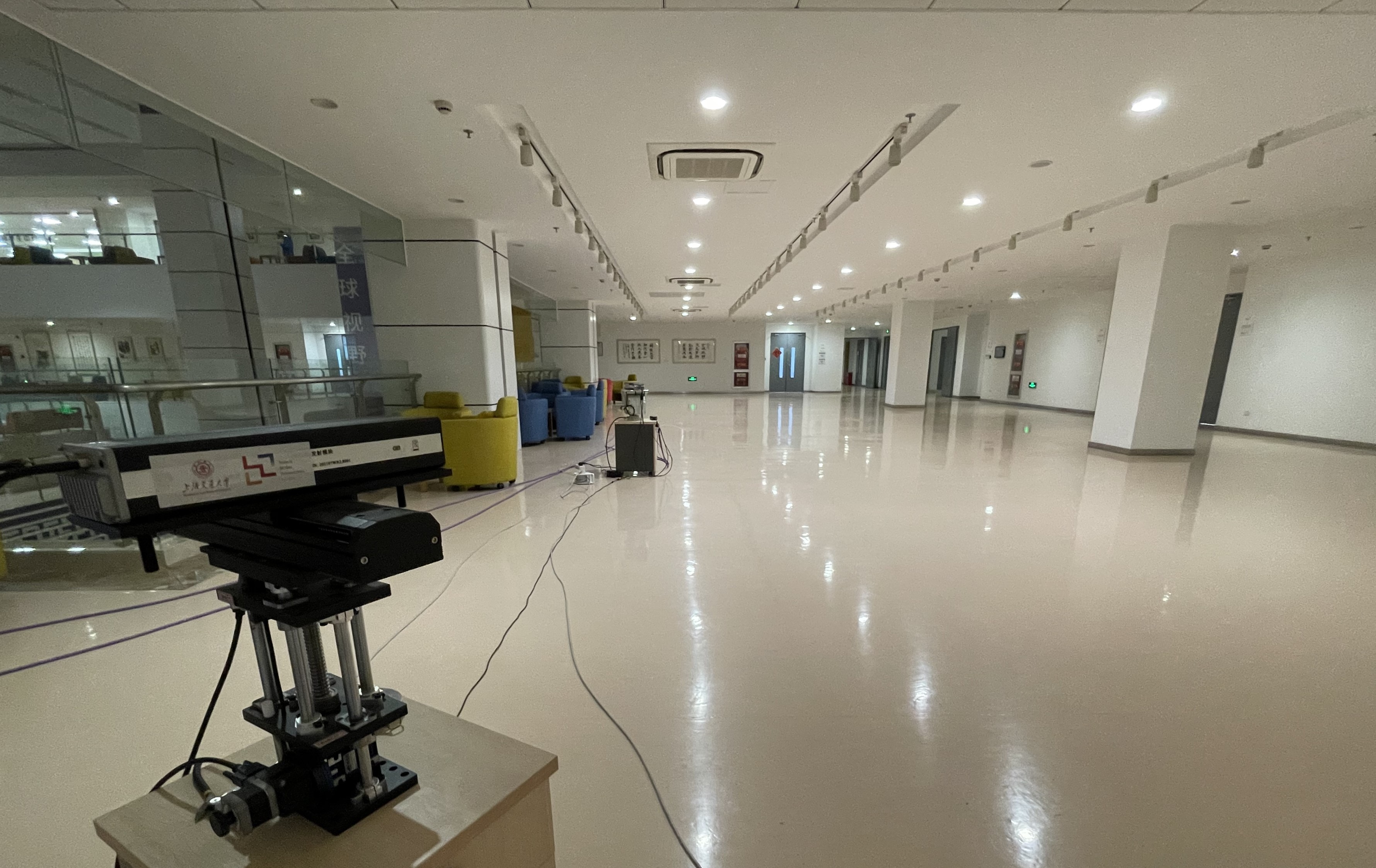
The THz MISO channel measurement system is composed of three parts, as shown in Fig. 9, including the computer (PC) as the control platform, the Ceyear 3672C vector network analyzer (VNA), the displacement platform carrying the THz transmitter (Tx) module, and the rotator carrying the THz receiver (Rx) module.
The measuring part consists of Tx and Rx modules and the VNA. The VNA generates radio frequency (RF) and local oscillator (LO) sources. The RF signal is multiplied by 27 to reach the carrier frequencies. The LO signal is multiplied by 24. As designed, the mixed intermediate frequency (IF) signal has a frequency of 7.6 MHz. Two IF signals at Tx and Rx modules, i.e., the reference IF signal and the test IF signal, are sent back to the VNA, and the transfer function of the device under test (DUT) is calculated as the ratio of the two frequency responses. The DUT contains not only the wireless channel, but also the device, cables, and waveguides. To eliminate their influence, the system calibration procedure is conducted, which is described in detail in our previous works [14, 15].
The mechanical part is composed of the displacement platform and the rotator. The displacement platform carries the Tx module to move linearly in the -axis (horizontally) and the -axis (vertically). The rotator carries the Rx module to scan the horizontal plane to receive angular-resolved multi-path components (MPCs). The PC alternately controls the movement of Tx through the displacement platform, the movement of Rx through the rotator, and the measuring process through the VNA. The measurement starts from the virtual antenna element in Tx at the left bottom corner, and all elements in the UPA are scanned first horizontally (in the -axis) and then vertically (in the -axis). At each element in Tx, the Rx scans horizontally and measures the THz channel once per angle.
IV-B Measurement Deployment
| Parameter | Measurement 1 | Measurement 2 | |
| Frequency band | 260-320 GHz | ||
| Bandwidth | 60 GHz | ||
| Time resolution | 16.7 ps | ||
| Space resolution | 5 mm | ||
| Sweeping interval | 30 MHz | 10 MHz | |
| Sweeping points | 2001 | 6001 | |
| Maximum excess delay | 33.3 ns | 100 ns | |
| Maximum path length | 10 m | 30 m | |
| Notation | Tx1-Rx1 | Tx2-Rx2 | Tx3-Rx3 |
| Tx gain / HPBW | 25 dBi / 8∘ | 7 dBi / 60∘ | |
| Tx antenna array type | 88 UPA | 22 UPA | |
| Tx antenna element spacing | 8 mm | 56 mm | 48 mm |
| Tx aperture size | 0.0792 m | 0.0679 m | |
| Rayleigh distance | 12.1259 m | 8.9088 m | |
| Rx gain / HPBW | 25 dBi / 8∘ | ||
| Rx angular scan | 0∘:2∘:90∘ | 0∘:2∘:358∘ | |
In this measurement, we investigate the THz frequency band ranging from 260 GHz to 320 GHz, which covers a substantially large bandwidth of 60 GHz. As a result, the time and space resolution is 16.7 ps and 5 mm, respectively. Key parameters of the measurement are summarized in Table IV.
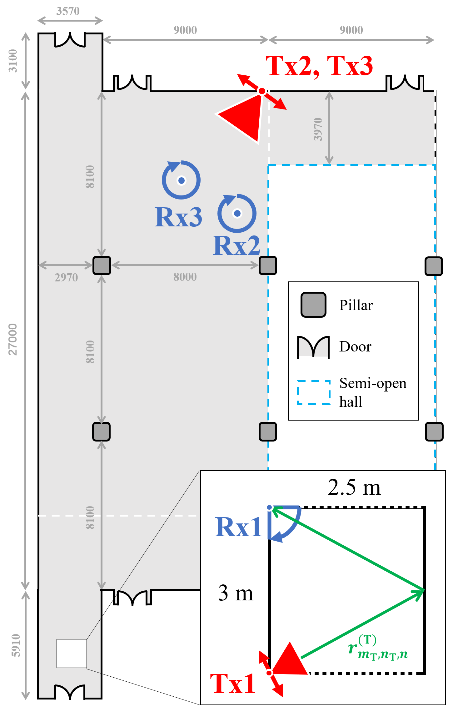
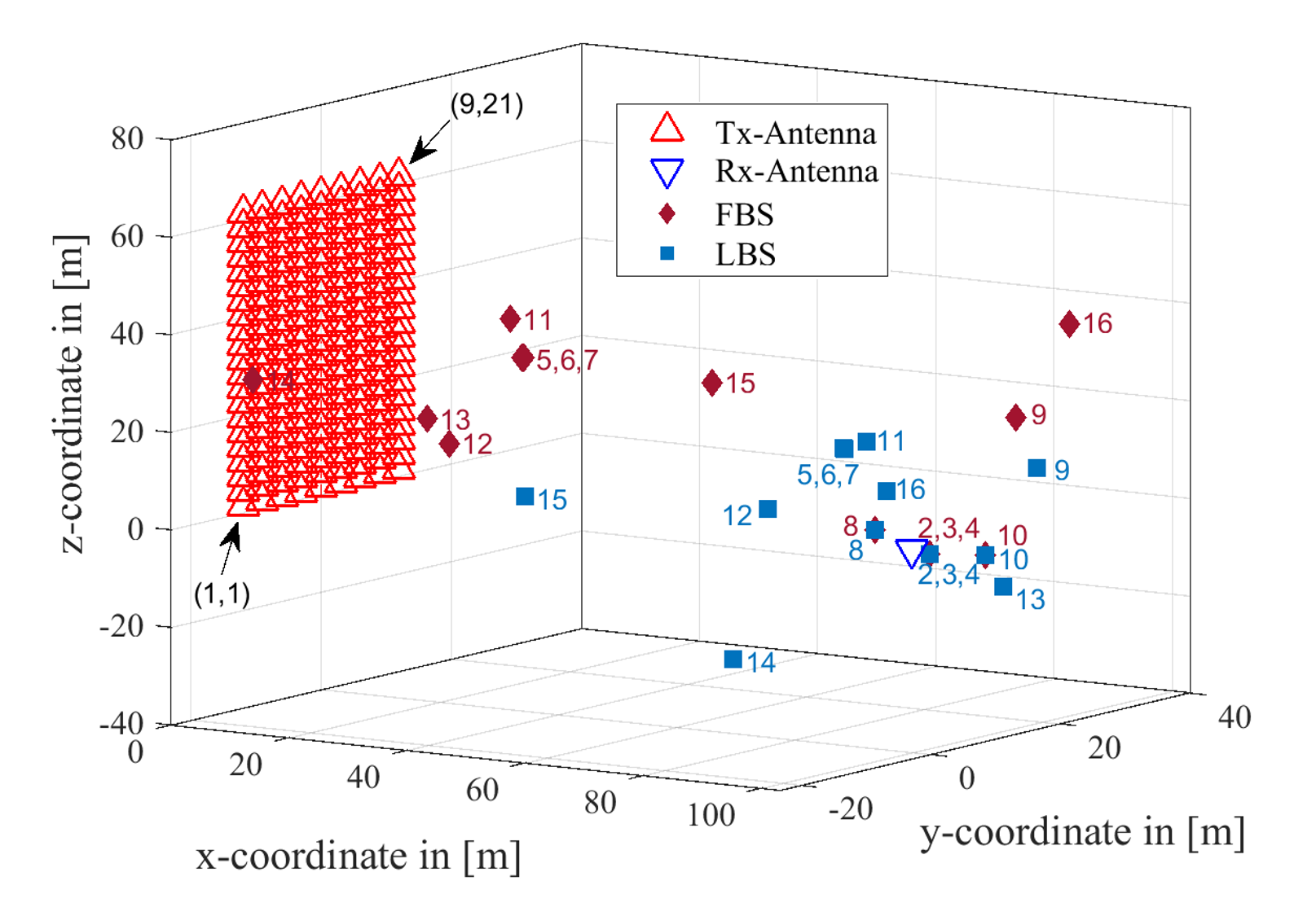
First, a small-scale measurement, from Tx1 to Rx1, is carried out, as shown in Fig. 10(b). The goal of the measurement is to investigate the cluster parameter from scatterers (the wall, in this deployment) in the near-field region. A virtual UPA with elements is measured at Tx, with the element spacing of 8 mm. In this case, the aperture size reaches 79.2 mm, which corresponds to the Rayleigh distance of 12.1259 m. The scale of the scenario is 2.5 m 3 m, which guarantees that the reflection happens in the near-field region. Furthermore, the small scale of the scenario enables the reduction of the maximum detectable path length to 10 m, corresponding to the frequency sweeping interval of 30 MHz and sweeping points of 2001 for each channel measurement. To increase the angular resolution, at Rx, the rotator scans from to with the step of . Furthermore, high-directive antennas are integrated at both Tx and Rx modules, with gains of around 25 dBi.
Then, another measurement is carried out in a larger-scale scenario, as shown by Tx2-Rx2 and Tx3-Rx3 in Fig. 10(a) and (b). Different from the setup in the first measurement, the maximum detectable path length is increased to 30 m, corresponding to the frequency sweeping interval of 10 MHz and sweeping points of 6001 for each channel measurement. Besides, the scan range of arrival angles covers to . Under this circumstance, the measuring time at each antenna element is multiplied by 12. Therefore, in this measurement, we decrease the number of virtual antenna element positions from 88 to 22, while the scale of the antenna array remains at 79.2 mm (and 67.9 m for comparison). Moreover, another antenna with a larger half-power beamwidth (HPBW), , is equipped at Tx.
IV-C Measurement Results
IV-C1 Measurement 1
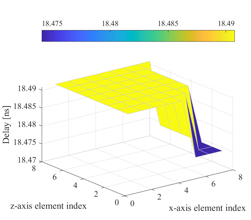
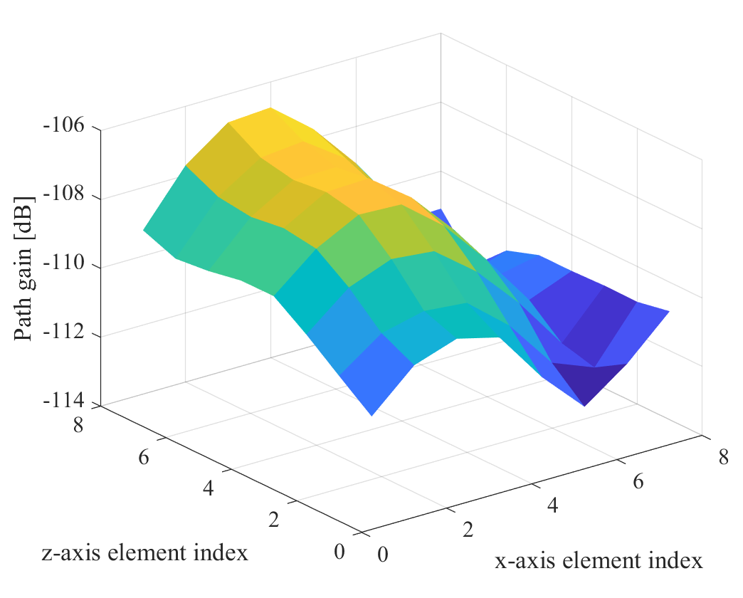
The sample with the greatest path gain in the PDAP is regarded as the wall-reflected ray from the Tx to the Rx. Fig. 11 illustrates the variation, across elements in the UPA, of delay, arrival angle, and path gain of the wall-reflected ray, respectively. First, due to symmetry, the distance from each element at Tx to the scatterer is half of the total path length. As shown in Fig. 11(a), the variation in distance from elements at Tx to the scatterer exceeds 2.5 mm, which is half of the path length resolution. The deviation is larger than of the wavelength, 0.065 mm, which accords with the analysis in the near-field region as summarized in Table III.
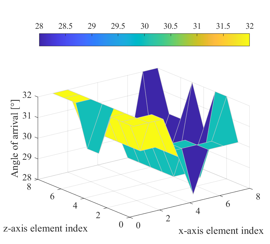
Second, the theoretical variation in the departure angle is about across 64 elements at Tx. Due to the reflection, scattering, and influence of antenna radiation patterns, the variation in the arrival angle reaches and results in a -dB variation in path gain of the measured MPC, as shown in Fig. 11(b) and (c). Despite the inevitable superposition of power inside the received beam in the practical measurement, in the simulation of cross-field channels, the departure/arrival angle of the MPC should still be carefully modeled when scatterers are in the near-field region, as the antenna gain differs in the antenna radiation pattern at different angles.
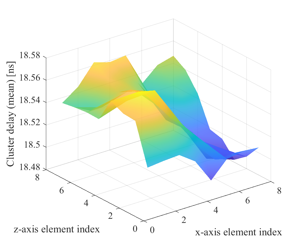
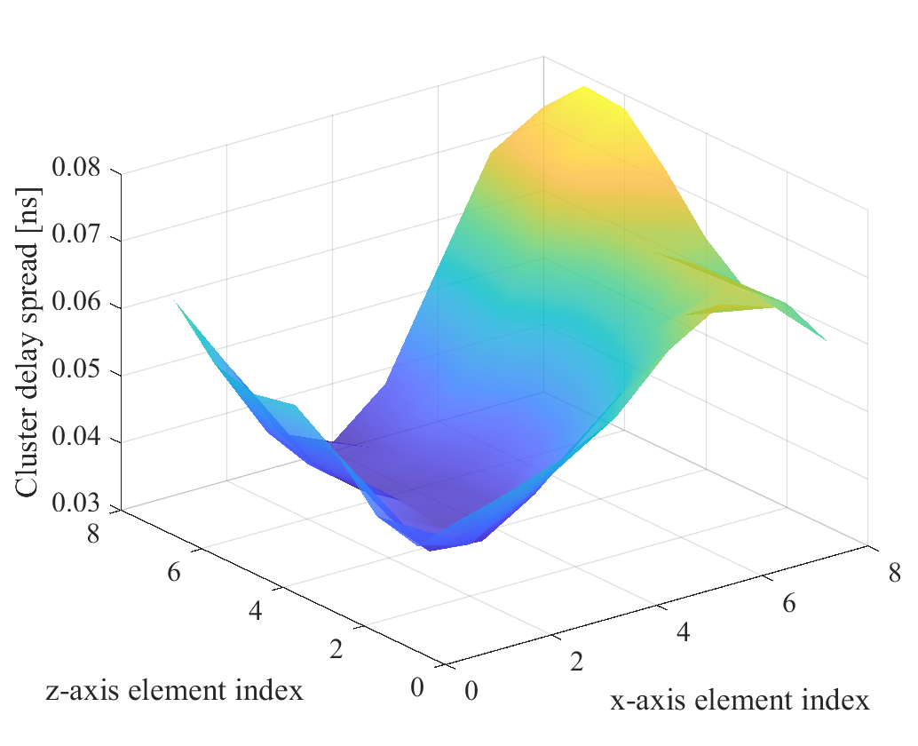
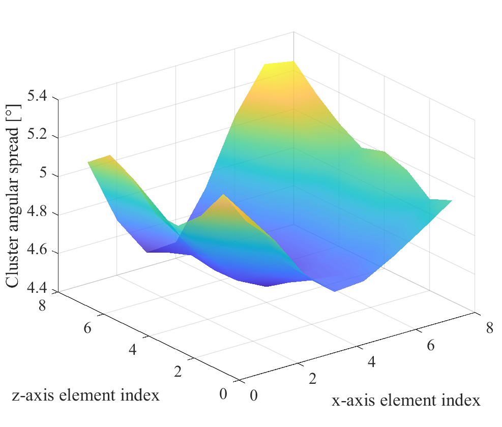
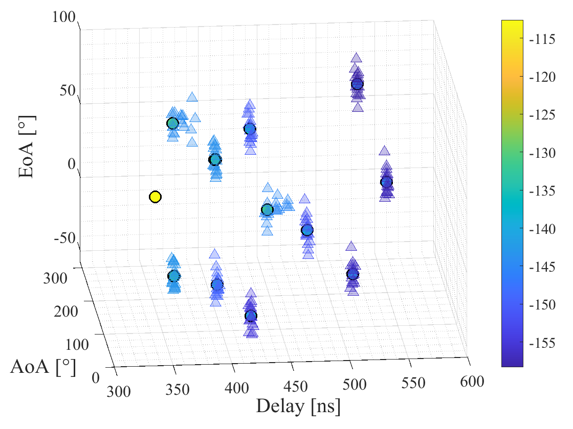
Furthermore, considering the cluster of MPCs around the wall-reflected ray, cluster parameters also vary across different elements at Tx, as summarized in Fig. 12.
IV-C2 Measurement 2
In the measurement in a larger indoor scenario, power-delay-angle profiles (PDAPs) are basically the same at four Tx antenna elements for Tx2-Rx2 and Tx3-Rx3 channels, respectively. 8-14 clusters are observed from Tx2 to Rx2, and 9-13 clusters are observed from Tx3 to Rx3, while the difference in the number of clusters comes from the difference in received power and the classification method which distinguishes MPCs and noise samples by thresholding [14].
The channel from the th antenna element at Tx to the Rx () is represented by , complex gain. We denote , and calculate the transmitter spatial correlation matrix as
| (29) |
where is the complex conjugate transpose of the matrix. where is the Frobenius norm. Assume there are adequate antennas at the receiver, the effective degrees of freedom (EDoF) is constrained by the transmitter spatial correlation matrix, which is calculated by
| (30) |
The Rayleigh distance is 12.1 m for the antenna array at Tx2, and the counterpart is 8.9 m for the antenna array at Tx3. According to the PDAP results, more scatterers are located in the NF region for Tx2-Rx2 transmission than for Tx3-Rx3 transmission. Correspondingly, the EDoF constrained by the Tx antenna array is 3.3460 for Tx2, and the counterpart is 3.3031 for Tx3, which are close to 4, the number of antenna elements at Tx. These values indicate the low correlation between antenna elements at Tx for near-field and cross-field channels, and the necessity of element-level modeling of channels with scatterers in the near-field region, even though the physical array size is small.
V Cross-field MIMO Channel Model Generation
In this section, detailed generation procedures of the cross-field MIMO channel model are described, and simulation results are discussed.
V-A Generation Procedure
As illustrated in Figure 13, the procedure is based on the model in 3GPP TR 38.901, while modified steps are described as follows.
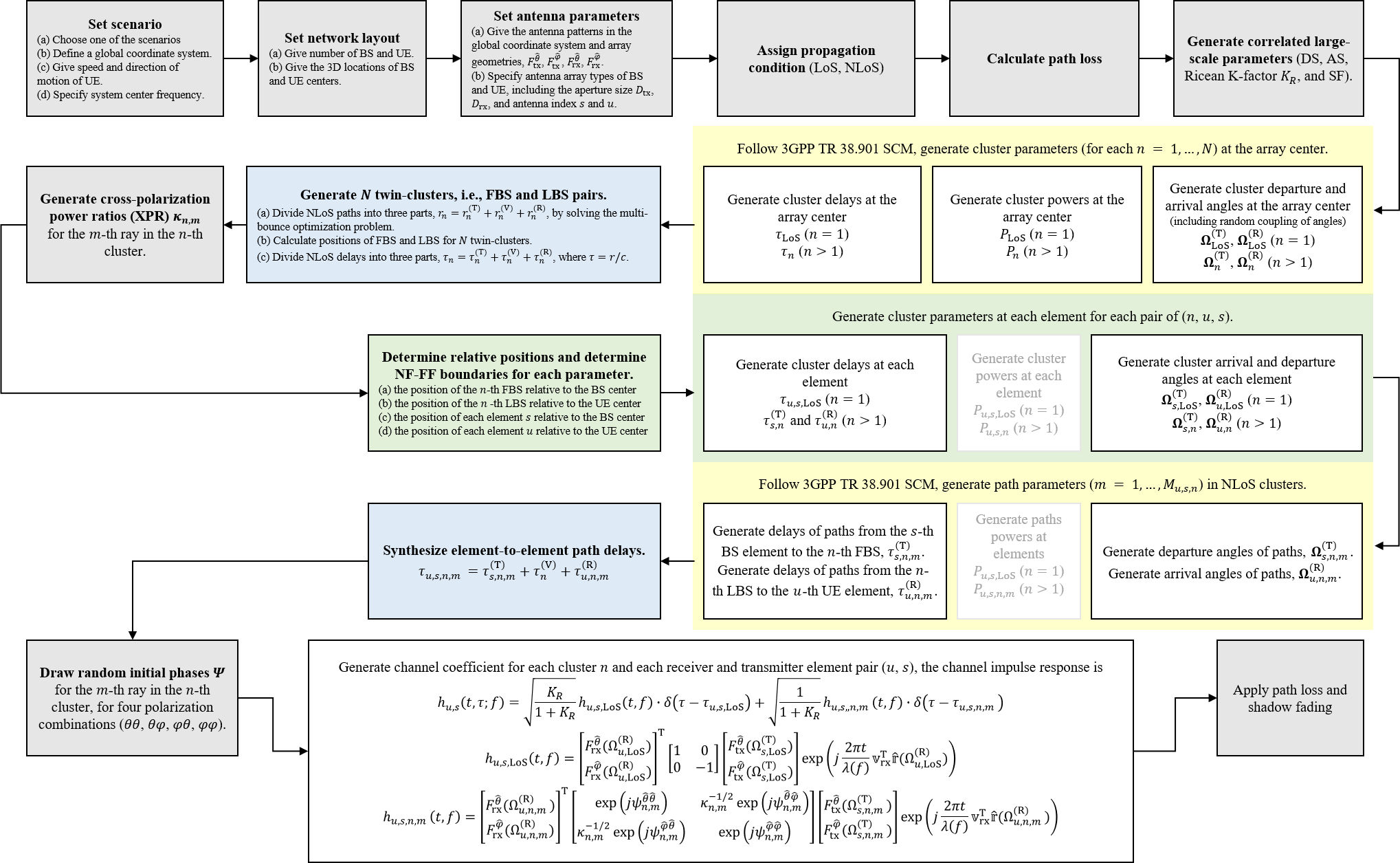
Step 7: Follow 3GPP TR 38.901 SCM, generate cluster parameters (), while includes (a) cluster delays, and , (b) cluster powers, and , and (c) cluster departure and arrival angles (including random coupling of angles), , , , .
Step 8: Generate twin scatterers, i.e., first-bounce-scatterer (FBS) and last-bounce-scatterer (LBS) pairs, while includes (a) divide NLoS paths into three parts, , by solving the multi-bounce optimization problem. (b) calculate positions of FBS and LBS for twin scatterers, and (c) divide NLoS delays into three parts, , where .
Step 10: Determine relative positions in the local coordinate system where the UPA lies in the -plane, including (a) the position of the th FBS relative to the BS center is denoted as , which is determined by length and angles . The corresponding unit vector is denoted as , and , (b) the position of the th LBS relative to the UE center is denoted as , which is determined by length and angles . The corresponding unit vector is denoted as , and , (c) the position of each element relative to the BS center, , is determined by the array structure, and (d) the position of each element relative to the UE center, , is determined by the array structure.
Step 11: Generate cluster delays at each element, , and . For the distance between the th FBS and the th BS element, , and the distance between the th LBS and the th UE element, , conduct the following steps respectively. (Take as example) If ,
| (31) |
otherwise, if ,
| (32) |
otherwise, accurately calculate . Finally, .
Step 12: Generate cluster arrival and departure angles at each element , , , and . For the elevation angle of departure from the th BS element to the th FBS and the elevation angle of arrival from the th LBS to the th UE element . (Take as example) If
then
| (33) |
otherwise, accurately calculate
| (34) |
where , , represent the coordinate of the vector in the Cartesian LCS. For the azimuth angle of departure from the th BS element to the th FBS and the azimuth angle of arrival from the th LBS to the th UE element . (Take as example) If
then
| (35) |
otherwise, accurately calculate
| (36) |
Step 13: Follow 3GPP TR 38.901 SCM, generate path parameters () in NLoS clusters at each (,) pair and (,) pair, including (a) delays of paths () from the th BS element to the th FBS, , (b) delays of paths () from the th LBS to the th UE element, , (c) departure angles of paths, , and (d) arrival angles of paths, .
Step 14: Synthesize element-to-element path delays by .
V-B Simulation Results
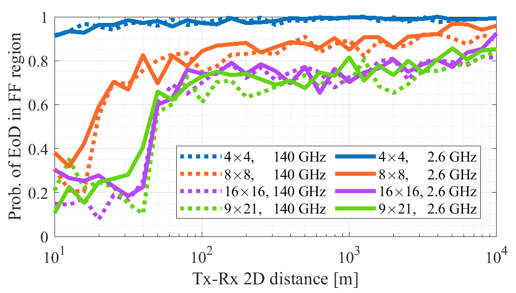
We first measures the statistical probabilities for the scatter to be in the near-field of the antenna array, in terms of MPC parameters, namely the delay and angles. Following the procedure described in Section V-A, we simulate the MISO channel in a UMa scenario at 2.6 GHz and 140 GHz. The Rx’s height is 2.5 m. Four types of antenna array are equipped at Tx respectively, namely , , , and UPA. The antenna element spacing is 3 m, much larger than the wavelength, and thus the largest two ELAAs span an area of 45 m 45 m, and 24 m 60 m. The center of the Tx array is 25 m high for , , and UPA. The UPA represents the scenario where antennas are hidden in construction elements [16]. In this case, the height of the Tx array center is 31.5 m to ensure that every antenna element is higher than Rx. We simulate each antenna element as a custom antenna with 3-dB beamwidth of both vertically and horizontally.
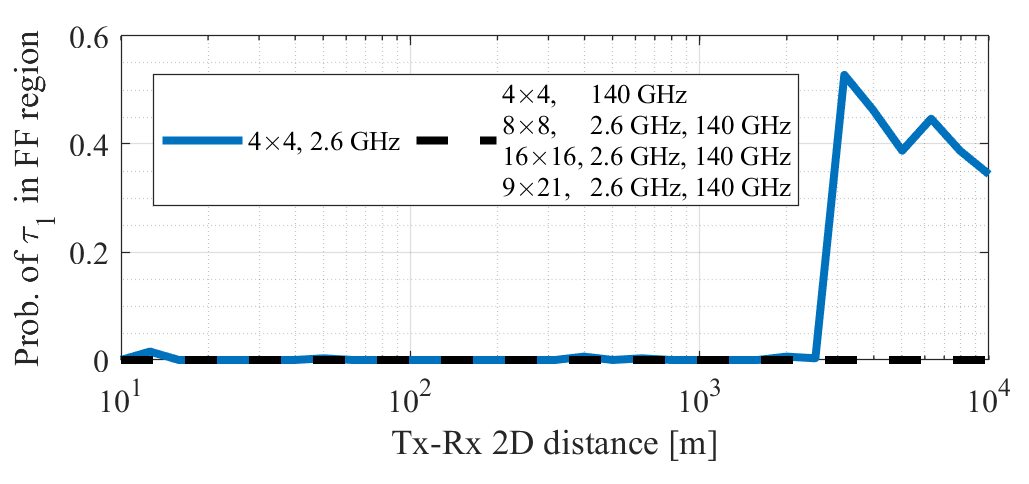
Fig. 14 shows one of the simulation results. In each trial, 15 pair of twin scatterers are generated, and the simulation with the same setup is repeated by 20 times. We calculate the statistical probability for the FBS located in the FF region, with respect to the path length from Tx antenna to FBS (or ), the azimuth angle of departure (AoD), and the elevation angle of departure (EoD), respectively. The 2D Tx-Rx distance, varies from 10 m to 10 km.
The results are summarized as follows. First, the FBS is always in the FF region in terms of AoD, and the value of AoD can be regarded as the same across the ELAA at either 2.6 GHz or 140 GHz.
Second, the probability that an FBS is in the FF region in terms of EoD becomes higher as Rx gets away from Tx. It is also verified that the NF-FF boundary in terms of angles is unrelated with the carrier frequency. More specifically, as shown in Fig. 15(a), at a certain range of , the FF probability rises rapidly and then saturates. Besides, the larger the antenna aperture size, the lower the likelihood that an FBS is in the FF region where the EoD from the Tx to the FBS should be calculated element-by-element. For instance, for ELAA than spans 45 m 45 m ( UPA) or 24 m 60 m ( UPA), when the 2D Tx-Rx distance is 30 m, 70%-80% of the FBS are in the NF region.
Third, as shown in Fig. 15(b), in all cases at 140 GHz, FBS is in the NF region of the Tx antenna array in terms of delay or path length. By contrast, at 2.6 GHz, the large wavelength narrows down the NF region. Even though, for the antenna aperture larger than 21 m 21 m ( UPA), all simulated FBS are located in the near-field region. In this case, the path length (or propagation time ) between the Tx antenna and the FBS should be calculated with a more accurate approximation. When the antenna aperture is reduced to 9 m 9 m ( UPA), and the 2D distance between Tx and Rx is larger than 3 km, there is a 40%-50% likelihood that an FBS falls in the FF region in terms of the path length (or propagation time ).
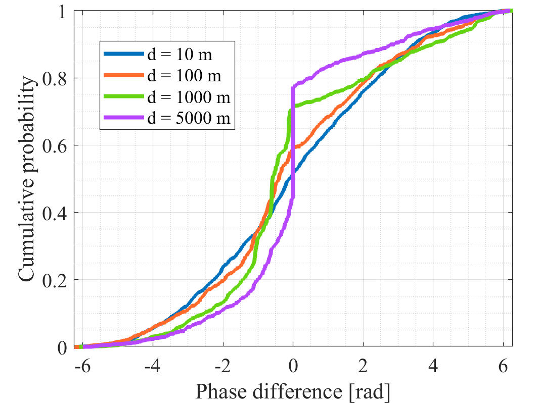
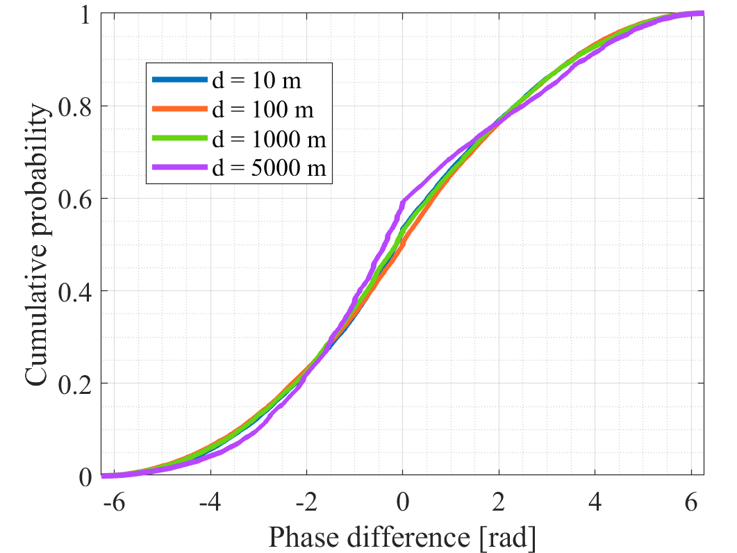
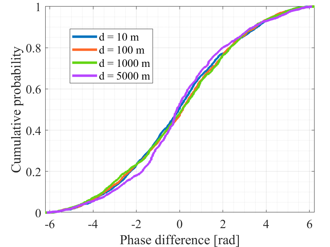
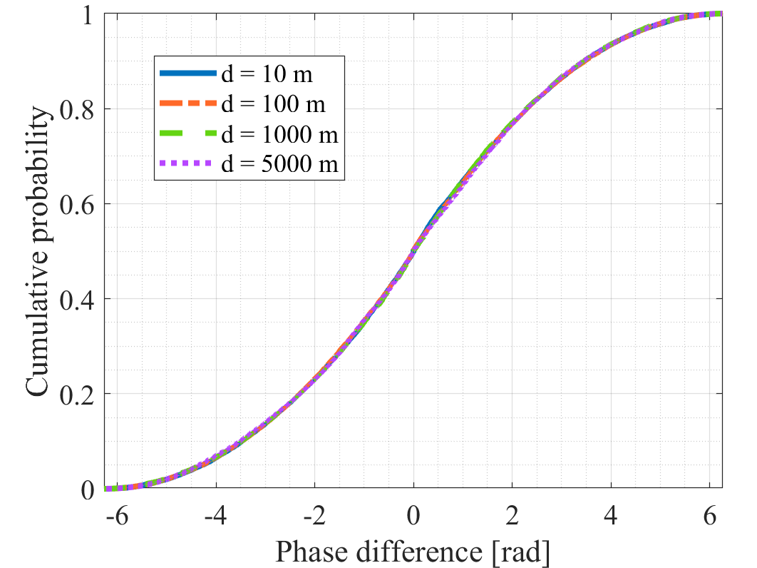
Then, we compare the proposed cross-field modeling with the far-field modeling of channels in ELAA systems. Fig. 16 shows the difference of phase for all paths and element-to-element links between CF and FF characterization. First, as the 2D distance between Tx and Rx increases, the phase difference between cross-field and pure far-field model is attenuated since there is a higher probability for scatterers to be located in the far-field. Second, as compared in Fig. 16(a)(b) and (c)(d), the larger the antenna array, the more the deviation between CF and FF modeling. Third, as compared in Fig. 16(a)(c) and (b)(d), the higher the frequency, the more the deviation between CF and FF modeling. Overall, as the cross-field phenomena become significant for ELAA systems, the distribution of phase difference tends to the normal distribution between and .
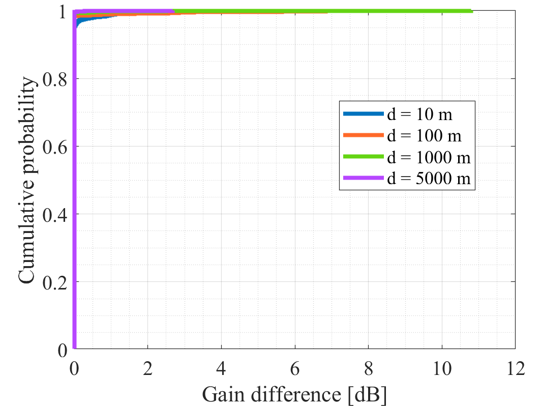
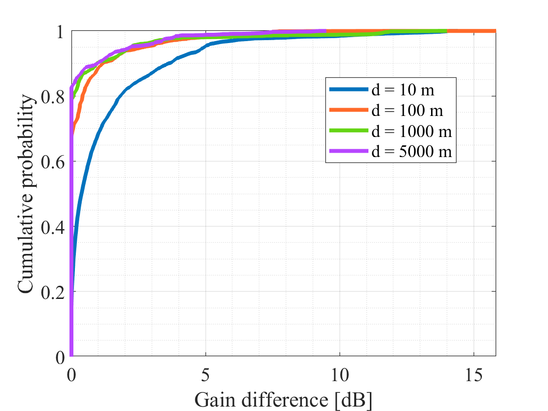
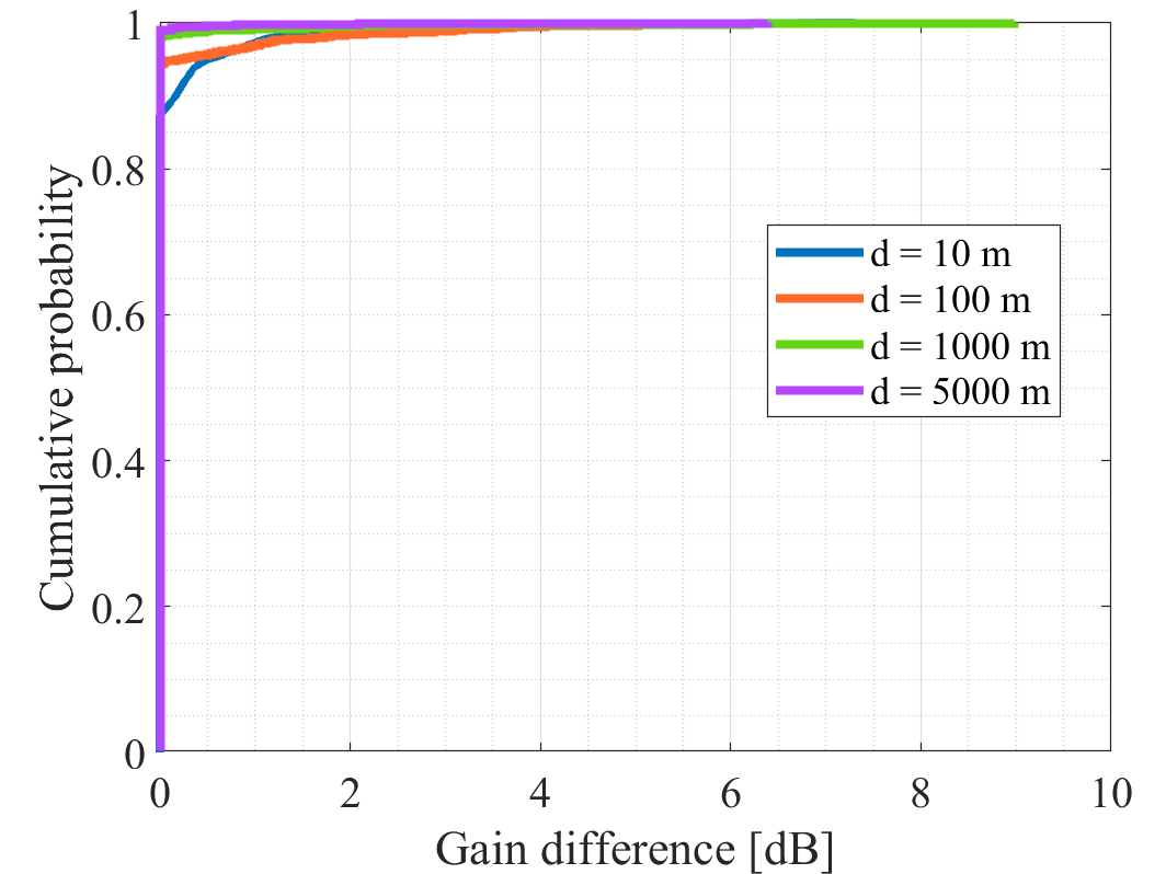
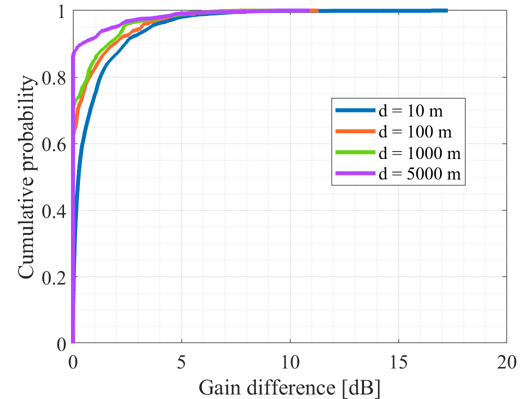
For the difference of gain for all paths and element-to-element links between CF and FF, as illustrated in Fig. 17. The size of antenna array is more significant then the frequency band. Still, the farther then distance, the less the difference between CF and FF characterization.
VI Conclusion
In this paper, we propose a cross near- and far-field MIMO channel model for ELAA systems. This starts with the introduction of the channel model framework based on twin-scatterer, i.e., the EM wave propagation is divided into three parts, separated by its first and last bounce. Then we provide a comprehensive analysis and closed-form expressions of cross-field boundaries and MPC parameters. By comparing the distance between the scatterer and the antenna array with the NF-FF boundary, far-field and near-field MPC parameters are generated separately. The analysis is verified by a cross-field channel measurement carried out in a small indoor scenario at 300 GHz, which also demonstrates the necessity of element-level modeling of MIMO channels when we have scatterers located in the near-field region. Furthermore, detailed channel generation procedures are provided, and simulations are conducted in a UMa scenario with , , , and UPAs at Tx at 2.6 GHz and 140 GHz. It turns out that element-level characterization of path length (or propagation time) in the near-field is indispensable for ELAA systems. Even for small antenna aperture like 9 m 9 m and 2D Tx-Rx distance larger than 3 km, there is also a 50%-60% likelihood that a scatterer falls in the near-field region in terms of the path length. By contrast, at least 70%-80% of elevation angle is in the near-field for ELAA systems that span as large as 45 m 45 m or 24 m 60 m when the 2D Tx-Rx distance is less than 30 m. Moreover, channel coefficients are compared between the proposed cross-field model and the original far-field model. While the difference in gain is limited to several decibels, the phase could deviate by at most a whole period of , which motivates the careful characterization of MPC parameters in cross-field modeling.
References
- [1] I. F. Akyildiz and J. M. Jornet, “Realizing ultra-massive MIMO (1024 1024) communication in the (0.06–10) terahertz band,” Nano Communication Networks, vol. 8, pp. 46–54, 2016.
- [2] W. Saad, M. Bennis, and M. Chen, “A Vision of 6G Wireless Systems: Applications, Trends, Technologies, and Open Research Problems,” IEEE Network, vol. 34, no. 3, pp. 134–142, 2020.
- [3] M. Cui, Z. Wu, Y. Lu, X. Wei, and L. Dai, “Near-field MIMO communications for 6G: Fundamentals, challenges, potentials, and future directions,” IEEE Communications Magazine, vol. 61, no. 1, pp. 40–46, 2022.
- [4] C. Han, Y. Wang, Y. Li, Y. Chen, N. A. Abbasi, T. Kürner, and A. F. Molisch, “Terahertz Wireless Channels: A Holistic Survey on Measurement, Modeling, and Analysis,” IEEE Communications Surveys & Tutorials, vol. 24, no. 3, pp. 1670–1707, Jun. 2022.
- [5] K. T. Selvan and R. Janaswamy, “Fraunhofer and Fresnel Distances: Unified derivation for aperture antennas,” IEEE Antennas and Propagation Magazine, vol. 59, no. 4, pp. 12–15, 2017.
- [6] H. Lu and Y. Zeng, “Communicating With Extremely Large-Scale Array/Surface: Unified Modeling and Performance Analysis,” IEEE Transactions on Wireless Communications, vol. 21, no. 6, pp. 4039–4053, 2022.
- [7] E. Björnson, Ö. T. Demir, and L. Sanguinetti, “A Primer on Near-Field Beamforming for Arrays and Reconfigurable Intelligent Surfaces,” in Proc. of Asilomar Conference on Signals, Systems, and Computers, pp. 105–112, 2021.
- [8] M. Cui, L. Dai, R. Schober, and L. Hanzo, “Near-Field Wideband Beamforming for Extremely Large Antenna Array,” arXiv preprint arXiv:2109.10054, 2021.
- [9] S. Sun, R. Li, X. Liu, L. Xue, C. Han, and M. Tao, “How to Differentiate between Near Field and Far Field: Revisiting the Rayleigh Distance,” arXiv preprint arXiv:2309.13238, 2023.
- [10] 3GPP, “Study on channel model for frequencies from 0.5 to 100 GHz,” 3rd Generation Partnership Project (3GPP), Technical Report (TR) 38.901, Dec. 2019, version 16.1.0.
- [11] Y. Chen, L. Yan, and C. Han, “Hybrid Spherical- and Planar-Wave Modeling and DCNN-Powered Estimation of Terahertz Ultra-Massive MIMO Channels,” IEEE Transactions on Communications, vol. 69, no. 10, pp. 7063–7076, 2021.
- [12] Y. Wang, S. Sun, and C. Han, “Far- and Near-Field Channel Measurements and Characterization in the Terahertz Band Using a Virtual Antenna Array,” IEEE Communications Letters, vol. 28, no. 5, pp. 1186–1190, 2024.
- [13] L. Xiao, Y. Xie, P. Wu, and J. Li, “Near-Field Gain Expression for Aperture Antenna and Its Application,” IEEE Antennas and Wireless Propagation Letters, vol. 20, no. 7, pp. 1225–1229, 2021.
- [14] Y. Wang, Y. Li, Y. Chen, Z. Yu, and C. Han, “0.3 THz Channel Measurement and Analysis in an L-shaped Indoor Hallway,” in Proc. of IEEE ICC, pp. 1–6, Jun. 2022.
- [15] Y. Li, Y. Wang, Y. Chen, Z. Yu, and C. Han, “Channel Measurement and Analysis in an Indoor Corridor Scenario at 300 GHz,” in Proc. of IEEE ICC, pp. 1–6, Jun. 2022.
- [16] E. Björnson, L. Sanguinetti, H. Wymeersch, J. Hoydis, and T. Marzetta, “Massive MIMO is a reality—What is next?” Digital Signal Processing, vol. 94, pp. 3–20, 06 2019.