Hidden Markov modelling of spatio-temporal dynamics of measles in 1750–1850 Finland
Abstract
Real world spatio-temporal datasets, and phenomena related to them, are often challenging to visualise or gain a general overview of. In order to summarise information encompassed in such data, we combine two well known statistical modelling methods. To account for the spatial dimension, we use the intrinsic modification of the conditional autoregression, and incorporate it with the hidden Markov model, allowing the spatial patterns to vary over time. We apply our method into parish register data considering deaths caused by measles in Finland in 1750–1850, and gain novel insight of previously undiscovered infection dynamics. Five distinctive, reoccurring states describing spatially and temporally differing infection burden and potential routes of spread are identified. We also find that there is a change in the occurrences of the most typical spatial patterns circa 1812, possibly due to changes in communication routes after major administrative transformations in Finland.
1 Introduction
Describing, visualising, and modelling spatio-temporal panel data is often challenging, particularly in high-dimensional settings with numerous time points and spatial areas. Conditional autoregressive models (CAR) (Besag,, 1974) and their variants, such as intrinsic conditional autoregressive models (ICAR), are frequently employed to describe areal data. Although it is possible to extend CAR models to spatio-temporal settings (Clayton and Bernardinelli,, 1996), these interaction models can become computationally intensive with high-dimensional data where spatial and temporal effects are not separable (Knorr-Held,, 2000). Approximate methods like INLA (Rue et al.,, 2009) may be computationally efficient alternatives to asymptotically exact Bayesian estimation via Markov chain Monte Carlo (MCMC), but these methods typically impose some restrictions on the model structure and the number of hyperparameters (Bakka et al.,, 2018). The potential bias of these approximations is also challenging to quantify in specific cases, although in many typical settings the approximation bias has been found to be negligible (Ogden,, 2016; Rue et al.,, 2017). Furthermore, visualising and interpreting the results of these interaction models may be complex: with time-varying spatial effects and a large number of time points, a substantial number of static maps are required to convey information about the estimated (or observed) spatial dynamics.
In life course research, hidden Markov models have been suggested as a probabilistic method to condense information of complex, multidomain life courses into a few interpretable latent states (Helske et al.,, 2018; Helske and Helske,, 2019). In these applications, given a common data generating process, individuals are assumed to be independent, having their own latent trajectories. In contrast, in spatio-temporal panel data, individuals share a spatial dependency structure which should be accounted for.
In Amorós et al., (2020), hidden Markov models are utilised in a spatio-temporal setting to detect influenza outbreaks, and in Knorr-Held and Richardson, (2003), they are used to identify meningococcal disease incidences. Both studies use two states to identify the endemic and epidemic, or endemic and hyperendemic, phases of the infections but do not aim to deeply analyse the underlying dynamics of the diseases. Employing more states may aid in discovering latent phenomena related to the epidemics. Amorós et al., (2020) include the spatial dependence in the epidemic state as temporally independent ICAR components and omit it in the endemic state, whereas Knorr-Held and Richardson, (2003) account for the spatial dependency as ICAR in both states but consider it as time-invariant.
In this paper, we propose a Bayesian hidden Markov model with a state-dependent spatial correlation structure as an unsupervised learning method for decomposing the spatio-temporal variation in the data into relatively few interpretable latent components. We illustrate our approach by modelling the spatio-temporal occurrence of measles in 18th- and 19th-century Finland.
Our model offers important insights into the historical measles epidemics in Finland. The extremely low population size coupled with hundreds of sparsely spaced small towns makes it challenging for epidemics to remain fully endemic (Keeling and Grenfell,, 1997). Thus, it is probable that fadeouts and reintroductions dominated the infection dynamics in Finland, implying that changes in the transmission sources could have strongly affected these dynamics. Finland and Sweden are separated by a large geographical barrier, the Gulf of Bothnia, and this, as well as the Russian border on the east, must have influenced the trade connections and the movement of people. The annexation of Finland to Russia, after a war in 1808–1809, resulted in the transfer of the capital from the western position of Turku to a more eastern location of Helsinki, increasing dramatically trade and social communication on the latter area, and drastically altering Finland’s connectivity to other countries (Ojala and Räihä,, 2017). We exploit our method to describe the reoccurring and presumably significantly foreign connection driven patterns of the epidemics in a compact yet informative way.
2 Data and methods
2.1 Data
Finland has a long history in collecting demographic and health-related data, with local parishes systematically maintaining records of baptisms, burials, and causes of death from 1749 onwards. Also earlier, albeit incomplete, records exist (Pitkänen,, 1977). Even though death diagnostics were symptom-based, the distinctive features of certain diseases allowed for relatively accurate diagnoses. One of those infections is measles, which we focus on. According to our data, measles accounted for approximately 2% of all deaths during our study period from 1750 to 1850. The population of Finland was roughly in 1750, and grew to over 1.6 million by 1850 (Tilastollinen päätoimisto,, 1899; Voutilainen et al.,, 2020). However, the healthcare system was primitive and virtually non-existent before the 19th century, lagging behind in development compared to the other Nordic countries and Europe until the 20th century (Saarivirta et al.,, 2009, 2012).
Communication within Finland and between neighbouring countries, combined with limited knowledge of infections and a poor healthcare system, were factors that enabled recurring epidemics of various diseases, including measles. While armed conflicts between countries were not uncommon, wars and border changes affected, among many other things, the common welfare of people. Finland had been part of Sweden for centuries, but already in 1721, Russia annexed the southeastern parts of Finland, or Old Finland, including the significant trading center of Vyborg. After the Finnish War in 1808–-1809, the rest of Finland became an autonomous grand duchy of Russia. In 1812, Old Finland was united with the new autonomous Finland, and the capital of Finland was moved from Turku on the southwestern coast to Helsinki on the southern coast, impacting markets and trade connections (Ojala and Räihä,, 2017). Being a remarkable transformation, the administrative change, however, left also many things unchanged. For example, the demographic records collected during the Swedish administration were still maintained in a similar way as before.
We analyse information obtained from parish records, using monthly data from January 1750 to December 1850 from different towns located in the southern half of Finland. The observations are dichotomous, indicating whether at least one death caused by measles was recorded. Thus, the data contains zeros for towns and months with no recorded deaths, and ones for those with recorded cases. Corresponding data, covering a different time span, has been used in Pasanen et al., (2023), which also describes the handling of the data in more detail. Other studies analysing data based on the same registers but covering different areas or time periods, or being aggregated to a different level, include, for example, Ketola et al., (2021) and Briga et al., (2021, 2022).
The data come with a significant amount of missing observations for several reasons. These include misdiagnoses, varying personal practices in maintaining the registers (Pitkänen,, 1977), and loss of records due to fires and other conditions over time. There are a total of time points, each having observations from – sites simultaneously, so no month has information from all the sites at once. From another perspective, only one town has no missing observations at all, whereas all observations are missing from towns. Overall, at the beginning of the time series, the missingness is approximately 70%, decreasing steadily to about 20% at the end of the time series, so that 40% of all data are missing.
2.2 Hidden Markov Models
Discrete time hidden Markov models (HMM) (Rabiner,, 1989) are statistical models for temporal, or other sequentially ordered data, consisting of two essential components. There are, firstly, the hidden stochastic Markov process describing the unobserved, yet often interesting, part of the model, and secondly, the observed process dependent on the hidden component. With the word ”state”, often appearing in the terminology, we refer to some discrete, prevailing situations related to the phenomenon of interest, for example, two states could be the presence and absence of a disease. Next, we introduce the method in more detail.
The first component of the model is the hidden stochastic process , with the state space , i.e., having values from to . Usually the temporal dependency of the process encompasses only one previous time point so that it satisfies the first-order Markov property
| (1) |
The hidden process may also meet some other order Markov condition, meaning that the current state depends on as many preceding states as is the degree of the Markov chain, but we do not consider those cases here. For the states we use consecutive numbering as labels for simplicity. Between two preceding time points it is possible to stay at the current state or to switch to another state. The probabilities of different transitions between the states are collected into a transition matrix , where each element where Additionally, initial state probabilities , describe the probabilities to start from each state at the first time point .
As a second component, we have the observed process , , where depends only on the current state of the hidden process. In consequence, the observations are conditionally independent:
| (2) |
Each state is associated with parameters of the observational distribution and thus we can also write . Of the parameters some may depend on the value of the state , while others may be shared between the states. Finally, we can define an emission matrix , where . Now the HMM can be defined by the set .
Often the hidden process and state-dependent parameters, describing the features of particular states, are the main interest of hidden Markov modelling, but since we do not directly observe the hidden process, we have to estimate it based on the observations gained from the non-hidden process. The general idea of the dependencies between the states, parameters and observations in HMMs is visualised in Figure 1.
While various methods have been suggested for estimating the number of states, , for example, Pohle et al., (2017), typically it is treated as known, fixed value when analysing the HMM results. The interpretation (”labelling”) of the hidden states is then based on the estimated model parameters , and on the hidden state trajectory , given the observations . As an example, consider HMM consisting of binary observations and two states, with , , , , and . From these, we see that we always start from state one which is relatively persistent state () emitting mostly zeros, whereas we are more likely to observe ones when the hidden process is in state two. Based on this, if the observations were related, for example, to the occurrence of some disease, we could label the first state as endemic state and the second state as epidemic state. We could also gain further understanding from the estimated state trajectory, from which we could see, for example, that state one is more common during winter, whereas state two occurs only during summer months. This could lead us to conclude that the transmission probability of our disease is higher during summer than winter, and thus further guide us to find reasons for that.
To perform fully Bayesian estimation of the HMM parameters and the corresponding latent states, we first run an MCMC targeting the marginal posterior of the model parameters, , where . For this we need the marginal likelihood , which can be computed with the forward part of the forward-backward algorithm (Baum and Petrie,, 1966; Rabiner,, 1989, and the references therein). The latent states can then be sampled in the post-processing stage given the posterior samples of . This marginalisation approach commonly used with latent variable models allows much more efficient sampling than the approaches where the estimation is based on the joint posterior , and is also strictly necessary when using efficient Hamiltonian Monte Carlo type of MCMC algorithms which rely on the differentiability of the posterior.
The marginal likelihood approach is also convenient with respect to missing data. When computing the emission probabilities , i.e., the conditional probabilities of the observations given the current state and the model parameters, we set for all if the observation is missing. This means that as we do not gain any new information about the states due to the missing observation at time , we essentially skip the contribution of at the marginal likelihood computation in forward algorithm at that time point (Zucchini and MacDonald,, 2009).
The likelihood and the posterior density of the hidden Markov models typically contain multiple modes. Some of these modes can be due to the label-switching problem (Jasra et al.,, 2005) but in complex models true local modes can also be present. In maximum likelihood setting the model parameters are often estimated by repeating the estimation several times with varying starting values for the optimisation algorithm, with the best solution declared as a global mode, while ignoring the other modes. In Bayesian setting multimodality of the posterior can pose both computational (convergence of the MCMC algorithms) and interpretability challenges. For example, it is difficult to interpret (label) and visualise the hidden states if the corresponding observational density is multimodal. These issues have to be taken into consideration when using HMMs.
The complexity of the response variables is not limited to scalars, but they can be multidimensional as well. In our case they are vectors containing spatially dependent elements. This means that the states, as well as the parameters, should allow for spatial structure.
2.3 Intrinsic conditional autoregressive models
Next we introduce the intrinsic conditional autoregressive (ICAR) model, which is a special case of the conditional autoregressive (CAR) model (Besag,, 1974), especially meant for spatial analysis to depict the amount of dependency between different locations. These models are based on a spatial division of a larger area, employing a neighbourhood definition for the generated subareas, and combining both of these with a Gaussian distribution in order to quantify the amount of the spatial dependency. This method does not offer information on the direction of the effects, i.e., the causal relationships, but only on the total amount of dependency.
For the spatial division, denote each areal unit or site of a regional entity with , and correspondingly its neighbour with . To account for the contiguity of the sites, let be an matrix for the binary neighbourhood so that the elements in it are
Additionally, denote with an diagonal matrix indicating the amounts of neighbours of each site so that
Now, we employ a variable to express the intensity of the dependency between each site and its neighbours. In case of the CAR model, we have
| (3) |
where the precision matrix has to be symmetric and positive definite for the distribution to have a proper joint probability density. This can be achieved with the matrices and by setting
| (4) |
where is a precision parameter of the variables , depicts the amount of spatial correlation, and is an identity matrix.
In case of ICAR model, we assume that , which results in improper distribution, which cannot be used as a model for the data, but as a prior distribution for spatial dependency, as is done for example in the Besag York Mollié (BYM) models (Besag et al.,, 1991). The parameters are not identifiable without further constraints, as adding a constant to all of them does not change their density. A common way to avoid the identifiability problem is to restrict them to sum to zero over the sites.
Some reasons to employ the improper distribution of ICAR instead of the proper of the CAR, are the facts that, firstly, to account significant amount of spatial association, the parameter most likely has to be close to one, and, secondly, the width of the posterior spatial pattern might be limited in the case of CAR (Banerjee et al.,, 2015). Thus, in some cases, it might be convenient to choose ICAR in the first place.
2.4 HMM with ICAR
In our approach, we combine the HMM and the spatial ICAR model, introduced above, thus enabling the HMM analysis of spatio-temporal data sets. We apply our method to the historical Finnish parish register data to study the dynamics of the measles epidemics. More precisely, our response variable is dichotomous, indicating the presence of at least one measles induced death observation in town in time point .
As before, we denote each site with , and each time point with . In this setting, the probability of observing at least one death caused by measles in site and time point can be modeled as
| (5) |
where the states
| (6) |
The notation means the row including all columns of the matrix . As we are using our method to study the occurrences and absences of deaths, Bernoulli distribution is a natural choice for the model. With other kinds of response variables also the distribution should be changed, for example Poisson distribution for counts. In formula 5, which corresponds to the in Equation 2, the logit link function maps the combination of the explanatory terms onto a probability scale required by the Bernoulli distribution. Also the link function should be changed to an appropriate one when using a different distribution. The four explanatory terms describe the state specific constants, the local constants, the intensity of spatial interaction between the site and its neighbours, and a monthly seasonal variation. The formula 6 defines the connection between the underlying states and the transition matrix .
The state specific constant , , sets a base level for the nationwide probability of observing at least one death in each state . In order to reduce the common, yet problematic, multimodality encountered with HMMs, we define the state specific constants so that they are monotonically increasing in a similar way as described in Bürkner and Charpentier, (2020). Due to this, our states are ordered based on the general incidence level. In our case, to begin with, we define the constants for the first and last state, and , respectively. We use these two to scale the ones for the other states. We do this by defining a simplex of S components, i.e., a vector summing to one, with the first term fixed to zero, and defining the rest of the constants as
| (7) |
As we are using a Bayesian approach, this allows us to employ informative priors for the constants of the first and last state, and .
To allow local deviations from the nationwide base level, we add a site dependent constant , which in turn is constant over the states. As we set the mean of the local constants to zero to improve model identifiability and MCMC sampling efficiency, we also gain a more straightforward interpretation of the state dependent constant as a nationwide average level. The local terms are not spatially dependent by definition, but aim to capture any heterogeneous features of the sites, for example, differing population sizes or communication intensities in our case.
The actual spatial dependence between the sites is introduced in the third term, . The dependency is achieved via the ICAR structure outlined above, i.e., adapting the formulas 3 and 4, and letting , where , and . To employ the ICAR component, we need a definition for the neighbourhood. Here two regions are considered as neighbours if they share a border. Other definitions, for example, based on the distance from the centers of the sites, could be used as well. In practice, the matrices and are constructed according to our neighbourhood definition in order to access the covariance of the spatial terms. The state specific spatial term is zero on average over the sites to guarantee identifiability using soft constraint as in Morris et al., (2019).
The final component in the model is a monthly average deviation additional to all the other components. It is constrained to sum to zero over a year.
As mentioned in subsection 2.1, our data are missing a large number of observations. However, as long as we assume they are missing at random, the HMM is a convenient approach to work with such imperfect data sets. Due to the hidden level, the observations do not depend on time, conditioned on the states, which is not the case when modelling dependencies only on the observed level. Now, the likelihood can be calculated without the missing observations by computing over only the observed sites at time . Thus, the absent information can be omitted while estimating the model, yet the model provides estimates for all sites and time points.
To fit the model we use a Bayesian approach, which on its behalf allows smooth handling of missing data and inclusion of prior information. This procedure requires setting prior distributions for the unknown parameters, and for the full model they are
where denotes a normal distribution truncated at , and denotes the components from to of the vector , omitting the first component since it is zero. The priors for the state specific constants and are chosen based on the data, to roughly match with the th and th percentiles of the monthly averages of the observed death occurrences. The row sums of the transition matrix are one, as well as the sums of the parameters and , which is achieved with the Dirichlet priors. In our case, the number of time points is and the number of sites . For our final model, we set the number of states to be .
3 Results
The model is estimated with MCMC using cmdstanr (Gabry and Češnovar,, 2022), which is an R interface (R Core Team,, 2023) for the probabilistic programming language Stan for statistical inference (Stan Development Team,, 2024). Posterior samples are drawn using NUTS sampler (Hoffman and Gelman,, 2014; Betancourt,, 2018) with four chains. Each chain consists of iterations, the first being discarded as warm-up. The computation with parallel chains takes approximately 30 hours. The estimation is done on a supercomputer node with four cores of Xeon Gold 6230 GHz processors, each core allocated GB of RAM. According to the MCMC diagnostics of the cmdstanr (Vehtari et al.,, 2021), the model converges without any divergences. The statistics are all below , and the bulk effective sample sizes are roughly between and , the most inefficient one being , which corresponds to a town and month that, while not associated with a missing observation itself, is missing five out of six of the neighbouring observations. The R and Stan codes and the data used for the analysis are available on GitHub (https://github.com/tihepasa/spatialHMM).
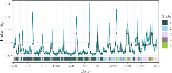
The data, aggregated temporally, the predicted probabilities of observing at least one death caused by measles, and the state trajectories that depict the path of the most probable states are illustrated in Figure 2. The predictions are computed according to the model as logit, followed by taking an average over all the sites. It appears that State 1 is predominantly prevalent before the year 1813, while States 2, 3 and 5 are emphasised during the remainder of the study period. State 5 emerges for the first time in 1793, whereas States 2 and 3 have a few occurrences since the beginning. State 4, on the other hand, appears throughout the whole study period. In general, State 1 is the most likely during % of the months, State 2 during % of the months, and States 3 and 4 during % and % of the months, respectively, leaving State 5 prevailing during % of the months. The probabilities of the estimated most likely states to be the actual most likely states always range between %, with approximately % of all of the probabilities being over %, and only five, randomly distributed in terms of time, falling below %.
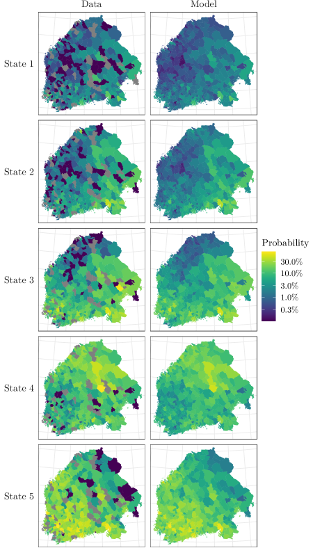
The spatial dimension of the states can be seen in Figure 3, which presents the estimated local probabilities and the corresponding data of observing at least one death caused by measles in each state. The probabilities are computed in accordance with the model, as in the temporal case above, aggregated over time, and displayed on a logarithmic scale to facilitate easier comparison both between and within the states. The smallest probabilities are associated with State 1, which seems to be common during the periods when the proportion of the observed deaths is low, see Figure 2. In States 1, 2 and 3, the probabilities seem to be larger in the southeastern parts of the country, and as moving from State 1 to the others the increased probabilities spread wider covering almost the whole study area in State 3. In State 4, the highest probabilities are located in the northern regions, and in State 5, they are concentrated in the southwestern half of the area.
According to the transition probabilities, shown in Table 1, it is most likely to remain in the current state. If we disregard this possibility, the most probable transitions are from State 1 to State 2, from State 2 to State 1, from States 3 and 4 to State 2, and from State 5 to State 4. The estimates of the initial state probabilities , along with other scalar parameters, can be found from Table 2. State 3 appears to be the starting point for the state trajectory in these data. However, the posterior distributions of the initial probabilities are quite wide. This is attributable to the fact that there is only one state trajectory to estimate, and an estimation based on a single observation does not provide much information.
| State 1 | State 2 | State 3 | State 4 | State 5 | |
|---|---|---|---|---|---|
| State 1 | 0.97 | 0.02 | 0.01 | 0.00 | 0.00 |
| (0.95, 0.98) | (0.01, 0.03) | (0.00, 0.02) | (0.00, 0.01) | (0.00, 0.01) | |
| State 2 | 0.04 | 0.91 | 0.02 | 0.02 | 0.00 |
| (0.02, 0.07) | (0.88, 0.95) | (0.01, 0.05) | (0.01, 0.04) | (0.00, 0.01) | |
| State 3 | 0.01 | 0.03 | 0.91 | 0.02 | 0.02 |
| (0.00, 0.03) | (0.01, 0.07) | (0.87, 0.95) | (0.01, 0.05) | (0.01, 0.05) | |
| State 4 | 0.02 | 0.05 | 0.02 | 0.89 | 0.02 |
| (0.00, 0.06) | (0.02, 0.10) | (0.00, 0.05) | (0.83, 0.93) | (0.00, 0.05) | |
| State 5 | 0.01 | 0.01 | 0.04 | 0.08 | 0.87 |
| (0.00, 0.03) | (0.00, 0.03) | (0.01, 0.010) | (0.03, 0.16) | (0.78, 0.94) |
The scalar constants , controlling the base levels of the probabilities to observe at least one death caused by measles in each state, are all negative in logit-scale and differ between the states distinctively, see Table 2. When these are transformed into a probability scale, the base probabilities range from % in State 1 to % in State 5.
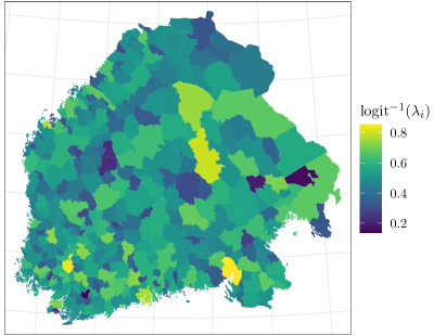
The local constants , independent of the state, are shown in Figure 4. As expected, there are no visible spatial patterns in these parameters aimed to capture spatially independent differences of the sites. The deviation of the constants is 0.59, see also Table 2, suggesting that there is some non-spatial heterogeneity between the towns. For instance, in State 5, the 5% and 95% quantiles for the posterior mean of the local probabilities are with median .
| mean | sd | 2.5% | 97.5% | ess bulk | ess tail | ||
|---|---|---|---|---|---|---|---|
| 0.17 | 0.14 | 0.01 | 0.52 | 17657 | 5620 | 1.00 | |
| 0.17 | 0.14 | 0.01 | 0.53 | 18953 | 5898 | 1.00 | |
| 0.33 | 0.18 | 0.05 | 0.73 | 20350 | 6151 | 1.00 | |
| 0.17 | 0.14 | 0.00 | 0.53 | 15146 | 6368 | 1.00 | |
| 0.17 | 0.14 | 0.01 | 0.53 | 16702 | 7113 | 1.00 | |
| -4.55 | 0.04 | -4.64 | -4.47 | 3595 | 5045 | 1.00 | |
| -3.87 | 0.04 | -3.96 | -3.79 | 4056 | 7210 | 1.00 | |
| -2.76 | 0.03 | -2.82 | -2.69 | 4229 | 6986 | 1.00 | |
| -2.43 | 0.03 | -2.49 | -2.36 | 1011 | 4169 | 1.00 | |
| -1.68 | 0.03 | -1.74 | -1.61 | 3109 | 5485 | 1.00 | |
| 0.59 | 0.03 | 0.53 | 0.65 | 2941 | 5410 | 1.00 | |
| 0.89 | 0.03 | 0.82 | 0.96 | 1368 | 2622 | 1.00 |
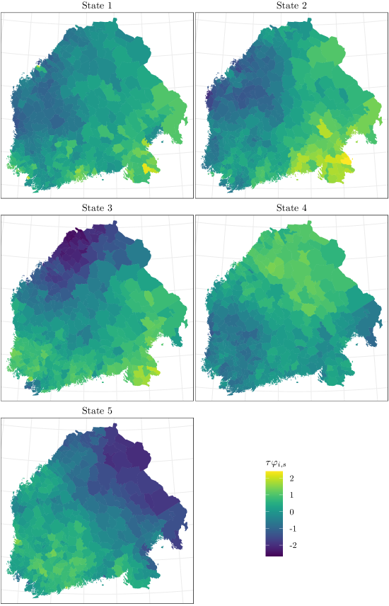
The spatial dependence in the spread of measles is accounted for by the spatial terms . The deviation parameter is constant for all the sites and states and is estimated to be , see also Table 2. The state-specific spatial terms are shown in Figure 5. The spatial patterns are similar to those of the estimated probabilities to observe at least one death caused by measles in Figure 3.
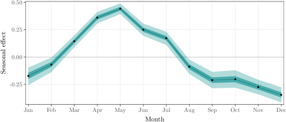
To capture the yearly temporal variation, the model includes a seasonal component , which is shown in Figure 6. These monthly terms sum to zero over a year, i.e., they depict an average monthly variation additional to the other components of the model. The effect of the month increases from January to peak in May and decreases after that until December. The effect is positive, thereby increasing the probability of observing a death caused by measles, from March to July, and negative or decreasing the risk otherwise. A somewhat similar pattern, with a peak in May, was also identified in (Pasanen et al.,, 2023) for measles during 1820–1850 in Finland.
While our HMM was estimated as homogeneous in terms of the transition matrix , Figure 2 suggests that the probability of observing deaths by measles changed around 1810. Before this, the hidden State 1 with the lowest baseline probabilities is the most prominent, after which the pattern of the hidden states appears to change considerably, both in terms of the baseline probability (transitioning from State 1 to State 2) and more frequent occurrences in the west coast (State 3). Therefore, as an additional analysis, we aimed to identify the most probable point in time where the spatio-temporal dynamics of measles changed regimes. For this purpose, we estimated a two-state left-to-right HMM, where the observations consisted of a thousand posterior samples of the state trajectories of our main model. All trajectories were modeled jointly so that they shared the same model parameters (state-specific categorical emission probabilities and the single transition probability from State 1 to State 2), but each trajectory had a separate hidden state process.
From the sampled state trajectories of this left-to-right model, we computed the distribution of the most probable change point, which was identified as November 1812 (with a 95% posterior interval from September 1812 to February 1813). Table 3 displays the estimated emission matrix of this model. From this, we can conclude that the major changes were the increased probabilities of States 2, 3, and 5 and the decreased probability of State 1 after November 1812. This finding aligns well with the associated administrative changes that led to transferring the capital towards the east, and to altering the trade connections (Ojala and Räihä,, 2017).
| State 1 | State 2 | State 3 | State 4 | State 5 | |
|---|---|---|---|---|---|
| Before | 0.69 | 0.12 | 0.05 | 0.11 | 0.02 |
| (0.69, 0.69) | (0.12, 0.13) | (0.05, 0.05) | (0.11, 0.12) | (0.02, 0.02) | |
| After | 0.04 | 0.39 | 0.34 | 0.14 | 0.09 |
| (0.04, 0.04) | (0.39, 0.39) | (0.33, 0.34) | (0.14, 0.14) | (0.09, 0.10) |
Determining the number of states in HMM is not a trivial task, and there is no definitive procedure for that, even though some suggestions exist (e.g., Pohle et al.,, 2017). In our case, we utilised five states, although a corresponding model was also estimated with four and six states. With six states there were several modes and convergence issues not only between but also within the chains. The model with four states, on the other hand, passed the convergence criteria but was not chosen here. Given that the states exhibited clear differences when there were five of them, we opted for the model with a greater number of hidden states. Presumably, this more detailed model also depicts the underlying phenomena more realistically in this context, since the epidemics are not discrete but continuous processes both in space and time.
For comparison, the supplementary material contains figures (Supplementary Figures 1–5) and tables (Supplementary Tables 1–2) for the four-state model, corresponding the ones represented here for the five-state model in Figures 2–6 and Tables 1–2. Based on Figures 2 and 3 and Supplementary Figures 1 and 2, it seems that States 1 and 2 of the five-state model have merged into State 1 of the four-state model, but otherwise the states correspond to each other.
4 Discussion
In this study, we illustrated the usage of the hidden Markov models in spatio-temporal analysis. Our aim was to gain information on the historical Finnish measles epidemics as a spatial and temporal process by modelling the probability of observing at least one death caused by measles in each town and month. The proposed HMM approach allowed us to summarise the information of data that are otherwise complicated and challenging to understand.
Using reported fatalities of measles in Finns throughout 1750–1850, and the Bayesian hidden Markov model with state-dependent spatial correlation structure, we identified five reoccurring epidemic states in Finland. The epidemics were characterised by two states of low burden of infection (States 1 and 2), and three states of higher infectious burden (States 3, 4 and 5), covering different parts of Finland (see Figure 3).
Our analyses revealed also a distinctive change in the epidemic dynamics between November 1812 and February 1813, matching well with the changes caused by the war between Sweden and Russia over the area of Finland in 1808–1809, and the imposed large administrative changes, including the transfer of the capital from Turku to Helsinki, in 1812. These transformations strengthened the eastern influence and trade connections (Ojala and Räihä,, 2017). The most notable change in the estimated state trajectory after the annexation of Finland by Russia was the replacement of State 1 with a generally higher death observation probability of State 2 as a non-epidemic state. Also the likelihood of States 3 and 5 increased, reflecting the higher infection burden at southern Finland and Karelian Isthmus, or south-western Finland, respectively. The view of the strengthened eastern influence is further supported by the increase of the infection burden especially in the eastern towns during the low epidemic states (Figure 3), possibly indicating persistent infectious pressure from the closest city in the area, Saint Petersburg. Overall, infections became more common across whole Finland after the war.
The dynamics of measles and other contagious infections are sensitive to population size (Keeling and Grenfell,, 1997). Due to the clear abrupt change in infection dynamics, we can perhaps safely rule out the role of gradual population increase (Voutilainen et al.,, 2020) here as the main driver of the change of the epidemics. Especially sparsely populated areas without endemic measles infections follow the changes of adjacent larger populations (Keeling and Grenfell,, 1997; Grenfell and Harwood,, 1997; Rohani et al.,, 2003; Ketola et al.,, 2021). Epidemics are affected by transport networks, geographical obstacles and borders (Vora et al.,, 2008). Finland and Sweden are separated by a large geographical barrier: The Gulf of Bothnia is 80–150 kilometers wide and 700 kilometers long, and obviously restricting the movement of people—and infections. Sea on the other side and the Russian border on the other side seem to have kept the infectious burden smaller in pre-war Finland compared with the post-war era when contacts to Russia and elsewhere increased (Ojala and Räihä,, 2017). During the history of nations, the borders have changed due to wars and the directions of transport and trade have shifted frequently, but the dynamics of epidemics due to such regime shifts have not been closely followed. Luckily, in our case, the administrative changes did not modify the data collection procedures of parishes so that we had data of the deaths available. This allowed us to study more closely the dynamics of epidemics due to changing transmission networks.
When it comes to the local transmission routes inside Finland, the definition of the proximity between the towns plays a crucial role. Other relevant definitions for the neighbourhood could be road or water connections instead of or in addition to the border sharing we used. As during longer time periods the areal structure is rarely static due to wars and other environmental changes, it would be interesting to extend the model into a case in which the spatial structure and neighbours can vary in time. This would require some further specifications for the state-specific spatial coefficients, as allowing several spatial structures within one state could result in having not only , but the number of different structures times , states. To set the specifications and try this kind of approach in practice, one should have further information about the spatial structure and the changes in it, but technically it could be implemented with our model. Additionally, within a fixed spatial structure one could estimate if some neighbouring towns did not interact at all so that there were actually discontinuities, as in Balocchi and Jensen, (2019).
As mentioned in section 1, there are several ways to model and estimate spatio-temporal connections. It would be natural to consider the phenomena as a continuous process instead of merely inspecting a collection of discrete states. One attractive way for this kind of more detailed analysis would be to fit a model without any hidden states, using random walks so that , where , and . In this case the spatio-temporal parameter may be seen as an interaction parameter of the temporal and spatial terms, as described for example in Clayton and Bernardinelli, (1996). However, given the large number of time points, spatial units, and iterations needed for the convergence of the MCMC, this kind of model is computationally infeasible to estimate in our case. Additional downside would be that due to the parameter profusion, the results would not be as interpretable or offer such a straightforward insight as our hidden Markov model.
We allowed for simplified, yet hopefully easy to understand, temporal dependency structure for the model via the parameters that depend on the state. Our method is especially convenient when there is a reason to suspect a presence of recurring patterns in the underlying phenomena. In other words, as we allow all potential transitions between our states so that it is possible to return to any of the previously occurred states later in time, also the latent process consists of repeated patterns. This enables finding the spatio-temporal epidemic dynamics and transmission routes illustrated by the repeated peak and fade-out patterns. In addition to the state-specific constants and spatial terms , also the local constant , deviation parameter and the seasonal term could depend on state if seen appropriate. To avoid multimodality and convergence problems, we did not include those further complexities in our model.
While our focus was on binary data, other observational distributions could be used and mixed, for example, a joint model of Poisson and Gaussian responses. There are previous indications of the profitability of the dichotomisation considering the last 30 years of our data (Pasanen et al.,, 2023). The model may also be extended to a case with exogenous covariates for the observational distributions or for the transition probabilities.
Acknowledgements
Tiia-Maria Pasanen was supported by the Finnish Cultural Foundation, the Emil Aaltonen Foundation and the Research Council of Finland grant 331817. Jouni Helske was supported by the Research Council of Finland grants 331817 and 355153. Tarmo Ketola was supported by the Research Council of Finland grant 278751. The authors wish to acknowledge CSC – IT Center for Science, Finland, for computational resources. The authors also thank Virpi Lummaa and Harri Högmander.
References
- Amorós et al., (2020) Amorós, R., Conesa, D., López-Quílez, A., and Martinez-Beneito, M.-A. (2020). A spatio-temporal hierarchical Markov switching model for the early detection of influenza outbreaks. Stochastic environmental research and risk assessment, 34(2):275–292.
- Bakka et al., (2018) Bakka, H., Rue, H., Fuglstad, G.-A., Riebler, A., Bolin, D., Illian, J., Krainski, E., Simpson, D., and Lindgren, F. (2018). Spatial modeling with R-INLA: A review. WIREs Computational Statistics, 10(6):e1443.
- Balocchi and Jensen, (2019) Balocchi, C. and Jensen, S. T. (2019). Spatial modeling of trends in crime over time in Philadelphia. The Annals of Applied Statistics, 13(4):2235–2259.
- Banerjee et al., (2015) Banerjee, S., Carlin, B., and Gelfand, A. (2015). Hierarchical Modeling and Analysis for Spatial Data, Second Edition. Chapman & Hall/CRC Monographs on Statistics & Applied Probability. Taylor & Francis.
- Baum and Petrie, (1966) Baum, L. E. and Petrie, T. (1966). Statistical inference for probabilistic functions of finite state Markov chains. The annals of mathematical statistics, 37(6):1554–1563.
- Besag, (1974) Besag, J. (1974). Spatial interaction and the statistical analysis of lattice systems. Journal of the Royal Statistical Society: Series B (Methodological), 36(2):192–225.
- Besag et al., (1991) Besag, J., York, J., and Mollié, A. (1991). Bayesian image restoration, with two applications in spatial statistics. Annals of the institute of statistical mathematics, 43:1–20.
- Betancourt, (2018) Betancourt, M. (2018). A Conceptual Introduction to Hamiltonian Monte Carlo.
- Briga et al., (2022) Briga, M., Ketola, T., and Lummaa, V. (2022). The epidemic dynamics of three childhood infections and the impact of first vaccination in 18th and 19th century Finland. medRxiv. [Preprint]. Posted October 31, 2022 [accessed May 25, 2023].
- Briga et al., (2021) Briga, M., Ukonaho, S., Pettay, J. E., Taylor, R. J., Ketola, T., and Lummaa, V. (2021). The seasonality of three childhood infections in a pre-industrial society without schools. medRxiv. [Preprint]. Posted October 18, 2021 [accessed September 29, 2023].
- Bürkner and Charpentier, (2020) Bürkner, P.-C. and Charpentier, E. (2020). Modelling monotonic effects of ordinal predictors in bayesian regression models. British Journal of Mathematical and Statistical Psychology, 73(3):420–451.
- Clayton and Bernardinelli, (1996) Clayton, D. and Bernardinelli, L. (1996). Bayesian methods for mapping disease risk. In Geographical and Environmental Epidemiology: Methods for Small Area Studies. Oxford University Press.
- Gabry and Češnovar, (2022) Gabry, J. and Češnovar, R. (2022). cmdstanr: R Interface to ’CmdStan’. https://mc-stan.org/cmdstanr/, https://discourse.mc-stan.org.
- Grenfell and Harwood, (1997) Grenfell, B. and Harwood, J. (1997). (Meta)population dynamics of infectious diseases. Trends in Ecology & Evolution, 12(10):395–399.
- Helske and Helske, (2019) Helske, S. and Helske, J. (2019). Mixture hidden Markov models for sequence data: The seqHMM package in R. Journal of Statistical Software, 88(3):1–32.
- Helske et al., (2018) Helske, S., Helske, J., and Eerola, M. (2018). Combining sequence analysis and hidden Markov models in the analysis of complex life sequence data. Sequence analysis and related approaches: Innovative methods and applications, pages 185–200.
- Hoffman and Gelman, (2014) Hoffman, M. D. and Gelman, A. (2014). The No-U-Turn sampler: Adaptively setting path lengths in Hamiltonian Monte Carlo. Journal of Machine Learning Research, 15(1):1593–1623.
- Jasra et al., (2005) Jasra, A., Holmes, C. C., and Stephens, D. A. (2005). Markov chain Monte Carlo methods and the label switching problem in Bayesian mixture modeling. Statistical Science, 20(1):50 – 67.
- Keeling and Grenfell, (1997) Keeling, M. J. and Grenfell, B. T. (1997). Disease Extinction and Community Size: Modeling the Persistence of Measles. Science, 275(5296):65–67.
- Ketola et al., (2021) Ketola, T., Briga, M., Honkola, T., and Lummaa, V. (2021). Town population size and structuring into villages and households drive infectious disease risks in pre-healthcare Finland. Proceedings of the Royal Society B: Biological Sciences, 288(1949):20210356.
- Knorr-Held, (2000) Knorr-Held, L. (2000). Bayesian modelling of inseparable space-time variation in disease risk. Statistics in Medicine, 19(17-18):2555–2567.
- Knorr-Held and Richardson, (2003) Knorr-Held, L. and Richardson, S. (2003). A hierarchical model for space–time surveillance data on meningococcal disease incidence. Journal of the Royal Statistical Society Series C: Applied Statistics, 52(2):169–183.
- Morris et al., (2019) Morris, M., Wheeler-Martin, K., Simpson, D., Mooney, S. J., Gelman, A., and DiMaggio, C. (2019). Bayesian hierarchical spatial models: Implementing the Besag York Mollié model in stan. Spatial and Spatio-temporal Epidemiology, 31:100301.
- Ogden, (2016) Ogden, H. (2016). On asymptotic validity of naive inference with an approximate likelihood.
- Ojala and Räihä, (2017) Ojala, J. and Räihä, A. (2017). Navigation Acts and the integration of North Baltic shipping in the early nineteenth century. International Journal of Maritime History, 29(1):26–43.
- Pasanen et al., (2023) Pasanen, T.-M., Helske, J., Högmander, H., and Ketola, T. (2023). Spatio-temporal modeling of co-dynamics of smallpox, measles and pertussis in pre-healthcare Finland.
- Pitkänen, (1977) Pitkänen, K. (1977). The reliability of the registration of births and deaths in Finland in the eighteenth and nineteenth centuries: Some examples. Scandinavian Economic History Review, 25(2):138–159.
- Pohle et al., (2017) Pohle, J., Langrock, R., Van Beest, F. M., and Schmidt, N. M. (2017). Selecting the number of states in hidden Markov models: pragmatic solutions illustrated using animal movement. Journal of Agricultural, Biological and Environmental Statistics, 22:270–293.
- R Core Team, (2023) R Core Team (2023). R: A Language and Environment for Statistical Computing. R Foundation for Statistical Computing, Vienna, Austria.
- Rabiner, (1989) Rabiner, L. R. (1989). A tutorial on hidden Markov models and selected applications in speech recognition. Proceedings of the IEEE, 77(2):257–286.
- Rohani et al., (2003) Rohani, P., Green, C., Mantilla-Beniers, N., and Grenfell, B. (2003). Ecological interference between fatal diseases. Nature, 422(6934):885–888.
- Rue et al., (2009) Rue, H., Martino, S., and Chopin, N. (2009). Approximate Bayesian inference for latent Gaussian models by using integrated nested Laplace approximations. Journal of the Royal Statistical Society: Series B (Statistical Methodology), 71(2):319–392.
- Rue et al., (2017) Rue, H., Riebler, A., Sørbye, S. H., Illian, J. B., Simpson, D. P., and Lindgren, F. K. (2017). Bayesian computing with inla: A review. Annual Review of Statistics and Its Application, 4(Volume 4, 2017):395–421.
- Saarivirta et al., (2009) Saarivirta, T., Consoli, D., and Dhondt, P. (2009). Suomen terveydenhuoltojärjestelmän ja sairaaloiden kehittyminen. Vaatimattomista oloista modernin terveydenhuollon eturintamaan. Kasvatus & Aika, 3(4).
- Saarivirta et al., (2012) Saarivirta, T., Consoli, D., and Dhondt, P. (2012). The evolution of the Finnish health-care system early 19th century and onwards. International Journal of Business and Social Sciences, 3(6):243–257.
- Stan Development Team, (2024) Stan Development Team (2024). Stan modeling language users guide and reference manual, version 2.34.
- Tilastollinen päätoimisto, (1899) Tilastollinen päätoimisto (1899). Pääpiirteet Suomen väestötilastosta vuosina 1750-1890: 1: Väestön tila. SVT: Suomen virallinen tilasto VI. Väkiluvun-tilastoa 29. Table 1 A.
- Vehtari et al., (2021) Vehtari, A., Gelman, A., Simpson, D., Carpenter, B., and Bürkner, P.-C. (2021). Rank-Normalization, Folding, and Localization: An Improved for Assessing Convergence of MCMC (with Discussion). Bayesian Analysis, 16(2):667–718.
- Vora et al., (2008) Vora, A., Burke, D. S., and Cummings, D. A. T. (2008). The impact of a physical geographic barrier on the dynamics of measles. Epidemiology and Infection, 136(5):713–720.
- Voutilainen et al., (2020) Voutilainen, M., Helske, J., and Högmander, H. (2020). A Bayesian reconstruction of a historical population in Finland, 1647–1850. Demography, 57(3):1171–1192.
- Zucchini and MacDonald, (2009) Zucchini, W. and MacDonald, I. (2009). Hidden Markov Models for Time Series: An Introduction Using R. Chapman and Hall/CRC.