Active gel model for one-dimensional cell migration coupling actin flow and adhesion dynamics

Abstract

Migration of animal cells is based on the interplay between actin polymerization at the front, adhesion along the cell-substrate interface, and actomyosin contractility at the back. Active gel theory has been used before to demonstrate that actomyosin contractility is sufficient for polarization and self-sustained cell migration in the absence of external cues, but did not consider the dynamics of adhesion. Likewise, migration models based on the mechanosensitive dynamics of adhesion receptors usually do not include the global dynamics of intracellular flow. Here we show that both aspects can be combined in a minimal active gel model for one-dimensional cell migration with dynamic adhesion. This model demonstrates that load sharing between the adhesion receptors leads to symmetry breaking, with stronger adhesion at the front, and that bistability of migration arises for intermediate adhesiveness. Local variations in adhesiveness are sufficient to switch between sessile and motile states, in qualitative agreement with experiments.

I Introduction

In multicellular organisms like ourselves, each and every cell has the ability to actively move Bodor et al. (2020). While cell migration of all cells plays an essential role during development, most cell types become quiescent in the mature organism, except for special situations like wound healing and immune surveillance. Reawakening of the ability of locomotion enables metastatic tumor cells to spread throughout the body Stuelten et al. (2018). Single-cell motility relies on the interplay between many proteins, but the main ones are filamentous actin, the motor protein non-muscle myosin II, and the adhesion receptors of the integrin-family. The main cellular processes contributing to cell migration are the formation of actin-driven protrusion at the leading edge, force transmission onto the substrate mediated by integrin-based cell-matrix adhesion, and retraction of the rear by actomyosin contraction Abercrombie (1980). It is a striking observation that single cells can switch between sessile and motile states and also between different directions of migration Verkhovsky et al. (1999); Ziebert et al. (2012); Lavi et al. (2016); Ron et al. (2020); Amiri et al. (2023). To explain this bistable migration behaviour in the absence of external cues, one has to identify the underlying mechanisms for spontaneous symmetry breaking (SSB).

To simplify both experimental observation and theoretical modeling, cells can be placed on one-dimensional (1D) tracks Maiuri et al. (2012, 2015); Hennig et al. (2020); Schreiber et al. (2021); Amiri et al. (2023), reducing the effective dimensionality of the problem. Such 1D tracks can be made e.g. with microcontact printing, laser lithography or microfluidics. A natural framework to describe cell migration in 1D is active gel theory Kruse et al. (2005); Jülicher et al. (2007); Prost et al. (2015). This model class can represent both polymerization and contractility in one coherent mathematical framework. In particular, active gel theory has been used to demonstrate that actomyosin contractility can be a mechanism for SSB that leads to self-sustrained cell motility, namely through an instability during which myosin localizes to the rear of the cell Recho et al. (2013). Due to the spatial nature of the model, intracellular flows and concentration fields are accessible and can be compared to experiments Recho et al. (2015). Furthermore, the effects of external perturbations, such as optogenetics Wittmann et al. (2020), can be incorporated into active gel models as local perturbations Drozdowski et al. (2021, 2023), again allowing for a comparison of experiment and theory.

An alternative mechanisms for SSB is the dynamics of adhesion. Adhesion receptors like the integrins are known to bind and rupture with mechanosensitive rates Humphrey et al. (2014). It is well known that non-linear adhesion rates lead to bifurcations in the adhesion dynamics Bell (1978); Erdmann and Schwarz (2004a), which in turn lead to non-trivial adhesion profiles and stick-slip motion of cell adhesion Sabass and Schwarz (2010); Schwarz and Safran (2013). In general, stick-slip motion is typical for sliding friction with non-linear dynamics Schallamach (1963); Filippov et al. (2004). Several bond models have been suggested to explain cell movement on 1D lines Sens (2020); Ron et al. (2020); Amiri et al. (2023). However, such models focus on the left and right cell edges and do not represent intracellular actin flow. The interplay between actin flow and adhesion dynamics is usually present in molecular clutch models Chan and Odde (2008); Bangasser et al. (2013); Oria et al. (2017); Elosegui-Artola et al. (2018); Alonso-Matilla et al. (2023), but this model class usually assumes that SSB has already occured and in general combines many individual rules to a complicated simulation framework.

Here we aim at representing both intracellular flow and adhesion dynamics in a transparent active gel model that allows us to perform a comprehensive mathematical analysis, using the powerful tools available for partial differential equations. Recently, a somewhat similar approach has been presented by extending the myosin-driven active gel model by adhesion dynamics, leading to oscillatory states and stick-slip migration Lo et al. (2024). However, in this model adhesion played only a minor role, while in practise, it might play a dominant role for SSB. Experimentally, it is not clear if one process dominates over the other. While some studies indicate that the cell front forms first via enhanced actin polymerization Pollard and Borisy (2003); Ridley et al. (2003), others suggest an increase in rear contractility as main mechanism Cramer (2010); Yam et al. (2007); Barnhart et al. (2015). In both cases, the onset of polarization is assigned to the actomyosin system. In contrast, Hennig et al. hypothesized that a spontaneous loss of adhesion at one cell edge is responsible for the observed sudden decrease in traction of cells on 1D tracks Hennig et al. (2020). This in turn causes the retraction of the prospective rear and initiates migration without pre-established cytoskeletal polarity.

To investigate the role of adhesion dynamics in the context of contractility-based cell migration, here we propose a minimal 1D active gel model in which an explicit adhesion field is coupled to the intracellular flow of actin. The adhesion density is treated as a reaction-diffusion system, where mechanosensitive bonds are subject to load sharing, which is known to be an essential non-linear effect leading to stick-slip in cell adhesion Bell (1978); Schwarz and Safran (2013). In combination with symmetric edge polymerization, this approach constitutes a minimal model for a novel and simple motility mechanism for 1D cell migration, where SSB results from the adhesion dynamics. For intermediate adhesiveness, robust motility exists in a bistable regime and our model predicts adhesion and intracellular flow profiles in very good agreement with experimental observations.

Having established this mechanism in our 1D-framework allows us to numerically study motility initiation by applying local perturbations to the adhesion density, similar to what has been demonstrated before for optogenetics Drozdowski et al. (2021, 2023). We show that nonlinear perturbations are required to switch from sessile to motile states and, in doing so, demonstrate the potential fundamental role of adhesion by forming the prospective rear. Furthermore, the interaction with a structured environment, e.g. a spatially varying concentration of ligands in the substrate, can be incorporated. In general, the model correctly recapitulates haptotactic behaviour Ricoult et al. (2015) and we describe its predictions for cells on patterned lines Schreiber et al. (2021); Amiri et al. (2023).

This work is structured as follows. In section II we introduce our model, derive consistent boundary conditions for the adhesion density and formulate a dimensionless boundary value problem (BVP). We then explain step-by-step the underlying polarization mechanism and how polarity is converted into directed migration by polymerization-driven flow. We show that active forces and adhesion-mediated friction have to be balanced and that motility is only possible in an intermediate regime of adhesiveness. In section III we analyse the effect of external perturbations, and in section IV we conduct a numerical study of cells on patterned lines to explore the full range of behaviour predicted by our model.

II Minimal model for adhesion-based motility

II.1 Model definition

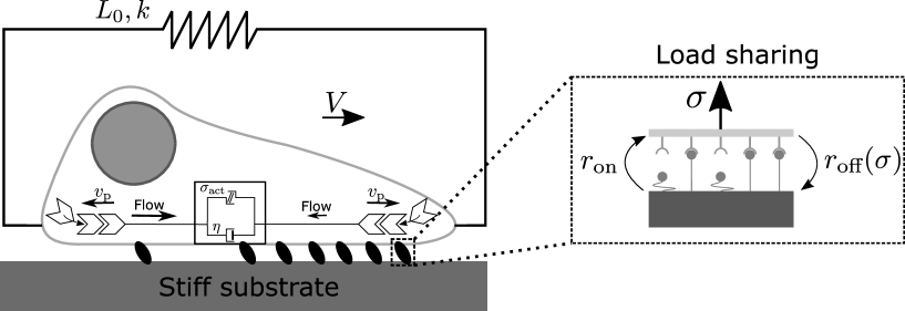
Figure 1: Schematic sketch of the 1D model: actomyosin contraction and edge polymerization of actin drive retrograde flow of a viscous bulk. Substrate friction is created by adhesion complexes, which are formed by binding/unbinding of mechanosensitive bonds, subject to load sharing, cf. the zoomed-in sketch. The cell length is a dynamic quantity and couples the two edges elastically.

In the following we aim to identify the minimal set of assumptions required to model the interplay between intracellular flow and adhesion during 1D cell migration. Fig. 1 sketches the main elements. We model the passive response of the cytoskeleton as a purely viscous, infinitely compressible fluid, which is locally subjected to an active stress $\sigma_{\rm{act}}$, modeling the effect of actomyosin contraction, which here is taken to be constant. The constitutive stress equation then reads

$$\sigma(x,t)=\eta\partial_{x}v(x,t)+\sigma_{\rm{act}},$$ (1)

with the viscosity $\eta$ and the actin flow velocity $v(x,t)$. In the molecular clutch model, the actin flow is coupled to the external substrate by receptor-ligand bonds mediated by proteins of the integrin-family, slowing down the retrograde flow and allowing for force transmission onto the substrate Chan and Odde (2008); Giannone et al. (2009); Oria et al. (2017). Assuming a linear relation between friction and local density of closed adhesion bonds $a(x,t)$ Sabass and Schwarz (2010); Ron et al. (2020); Schreiber et al. (2021), local force balance implies

$$\partial_{x}\sigma(x,t)=\xi v(x,t)\left(a_{0}+a(x,t)\right).$$ (2)

$\xi$ is an effective friction coefficient and $a_{0}$ represents a baseline level of friction caused by other, non-specific dissipative interactions between actin, membrane and substrate. Combining equations Eq. 1 and Eq. 2 yields a single stress equation

$$\frac{\eta}{\xi}\partial_{x}\left(\frac{\partial_{x}\sigma(x,t)}{a_{0}+a(x,t)}\right)=\sigma(x,t)-\sigma_{\rm{act}}.$$ (3)

Single integrin bonds cluster to focal complexes and mature into so-called focal adhesions by recruiting further adapter proteins. We use a reaction-diffusion system Barnhart et al. (2011); Löber et al. (2014) to describe the effective evolution of the adhesion density

$$\partial_{t}a(x,t)=r_{\rm{on}}-r_{\rm{off}}(x,t)a(x,t)+D\partial_{x}^{2}a(x,t).$$ (4)

In a coarse-grained manner, we assume a dense distribution of ligands on the substrate and describe adhesion as a continuous field. Because the plasma membrane acts as a reservoir for adhesion molecules, it is sufficient to only consider the density of closed bonds. They are assumed to attach with a constant rate $r_{\rm{on}}$, while the dissociation rate $r_{\rm{off}}$ is mechanosensitive and increases exponentially under load Bell (1978); Janeš et al. (2022). Using the principle of load sharing, the local stress is distributed among the bonds at each position, corresponding to the force per bond typically used in models for adhesion sites Bell (1978); Erdmann and Schwarz (2004a, b); Sens (2020), such that

$$r_{\rm{off}}(x,t)=r_{0}\ {\rm{exp}}\left(\frac{|\sigma(x,t)|}{f_{0}\left(a_{0}+a(x,t)\right)}\right).$$ (5)

A small decrease in $a$ increases the force per bond on the remaining ones, which in turn facilitates detachment and can result in a rupture cascade Erdmann and Schwarz (2004a, b). We assume here the same baseline friction $a_{0}$, avoiding a divergence of the off-rate for very small adhesion densities. $f_{0}$ represents the characteristic force scale at which single bonds tend to rupture. The off-rate without load is given by $r_{0}$.

The effective diffusion constant $D$ accounts for thermal fluctuations and steric effects due to the finite size of adhesion proteins. It stabilizes the system Barnhart et al. (2011); Löber et al. (2014) and ensures continuous adhesion profiles. However, compared to the binding processes, the effective diffusion should be slow. Because adhesions stay stationary relative to the substrate, while the migrating cell moves over them Zaidel-Bar et al. (2004), advection does not occur in the lab frame of reference.

To close the equations for stress and adhesion density, we have to formulate appropriate boundary conditions (BCs). Since we deal with a moving cell, the positions of the right and left boundary $l_{\pm}(t)$, corresponding to the cell edges, as well as the cell length, $L(t)=l_{+}(t)-l_{-}(t)$, will vary over time. However, due to volume regulation of cells, the typical cell size should not vary much. We therefore apply symmetric and elastic stress BCs Recho et al. (2013); Drozdowski et al. (2021)

$$\sigma(l_{\pm},t)=-k\frac{L(t)-L_{0}}{L_{0}},$$ (6)

with effective spring constant $k$ and reference length $L_{0}$, which both result from volume regulation.

Actin predominantly polymerizes in the vicinity of the plasma membrane, i.e. at the left and right boundaries in our model. Non-motile cells show symmetric polymerization that is matched by retrograde flow. In motile cells, polymerization induces membrane protrusions at the leading edge, while depolymerization is observed in the bulk and rear of the cell. Since our effective 1D description is an average over the height and width of the lamellipodium, we assume the same constant polymerization velocity $v_{\rm{p}}$ pointing outward at the two boundaries. Bulk depolymerization, which is necessary for conservation of total actin mass, is neglected Jülicher et al. (2007) in agreement with the assumptions of an infinitely compressible gel. Then, polymerization offsets the movement of the cell edges and the flow velocity of the gel like

$$\dot{l}_{\pm}(t)=v(l_{\pm},t)\pm v_{\rm{p}}.$$ (7)

Finally, starting from a system of reaction-diffusion equations for bound and unbound adhesion sites and assuming conservation of the total number of binding sites, we can derive BCs for $a(x,t)$ by taking the limit of an infinite reservoir of unbound sites (cf. A) and obtain

$$\partial_{x}a(l_{\pm},t)=-\frac{\dot{l}_{\pm}(t)}{D}a(l_{\pm},t).$$ (8)

Because closed bonds are not advected, but only diffuse, the ratio of edge movement and diffusion arises here.

II.2 Non-dimensionalisation

We non-dimensionalize the equations by rescaling length by $L_{0}$, time by the inverse off-rate without load $1/r_{0}$ , stress by the effective spring constant $k$, and adhesion density by $k/(L_{0}^{2}\xi r_{0})$. By transforming to the internal coordinate of the cell, $u=(x-l_{-})/L$, we can map the moving BVP to the unit interval with stationary boundaries. Then, the global movement of the cell is absorbed in the advection velocity field $\tilde{v}=\dot{G}/L+\dot{L}/L(u-1/2)$ with the cell’s center position $G=(l_{+}+l_{-})/2$. The full nondimensional BVP reads

$$\frac{\mathcal{L}^{2}}{L^{2}}\partial_{u}\frac{\partial_{u}\sigma(u,t)}{\mathcal{A}+a(u,t)}=\sigma(u,t)-\sigma_{\rm{act}},$$ (9)

$$\sigma(u_{\pm},t)=-(L(t)-1),$$ (10)

$$\dot{l}_{\pm}(t)=\frac{1}{L}\frac{\partial_{u}\sigma(u_{\pm},t)}{\mathcal{A}+a(u_{\pm},t)}\pm v_{\rm{p}},$$ (11)

$$\partial_{t}a(u,t)-\tilde{v}(u,t)\partial_{u}a(u,t)=\mathcal{R}-{\rm{exp}}{\left(\frac{1}{\mathcal{F}}\frac{|\sigma(u,t)|}{\mathcal{A}+a(u,t)}\right)}a(u,t)+\frac{\mathcal{D}}{L^{2}}\partial_{u}^{2}a(u,t),$$ (12)

$$\partial_{u}a(u_{\pm},t)=-\frac{La(u_{\pm},t)}{\mathcal{D}}\dot{l}_{\pm}(t).$$ (13)

In addition to $\sigma_{\rm{act}}$ and $v_{\rm{p}}$, our model is described by five dimensionless parameters: $\mathcal{L}=\sqrt{\eta r_{0}/k}$ describes the viscous time scale relative to the binding time. $\mathcal{R}=\xi L_{0}^{2}r_{\rm{on}}/k$ determines the binding rate. $\mathcal{F}=f_{0}/(\xi L_{0}^{2}r_{0})$ represent the typical rupture force of closed bonds and $\mathcal{A}=a_{0}\xi L_{0}^{2}r_{0}/k$ corresponds to the baseline friction. Lastly, $\mathcal{D}=D/(L_{0}^{2}r_{0})$ is the effective diffusion of closed bonds and should be small compared to $\mathcal{R}$.

For the remainder of this article, we use a dimensionless polymerization speed of $v_{\rm{p}}=0.1$, which corresponds to $0.1\ \mu$m/s as typical order of magnitude experimentally observed for various cell types Barnhart et al. (2011); Schreiber et al. (2021). The estimates of the other parameters are available in B and imply $\mathcal{L}=1.0$, $\sigma_{\rm{act}}=0.1$ and $\mathcal{F}=0.16$. The diffusion $\mathcal{D}$ and baseline friction $\mathcal{A}$ are effective parameters and cannot be directly inferred from experiments. They serve a regularizing function and, as we will show in the following section, should be sufficiently small. We use $\mathcal{D}=0.01$ and $\mathcal{A}=0.1$. $\mathcal{R}$ acts as main continuation parameter and is not fixed to a specific value. The expected value is of the order of one.

II.3 Adhesion-based mechanism for polarization

Without polymerization a homogeneous stress state, determined by the active stress $\sigma(u)=\sigma_{\rm{act}}$, satisfies equations Eq. 9 and Eq. 10 independently of the adhesion density. As a result, there is no actin flow, leading to $\dot{l}_{\pm}=0$ and $\tilde{v}=0$. The steady state of the adhesion is implicitly described by the equation

$$0=\mathcal{R}-{\rm{exp}}\left(\frac{1}{\mathcal{F}}\frac{\sigma_{\rm{act}}}{\mathcal{A}+a(u)}\right)a(u)+\frac{\mathcal{D}}{L^{2}}\partial_{u}^{2}a(u),$$ (14)

where the BCs simplify to $\partial_{u}a(u_{\pm})=0$. First, we analyse uniform solutions, $\partial_{u}a=0$, such that the diffusion term vanishes. Eq. 14 then characterizes the local balance of binding and unbinding.

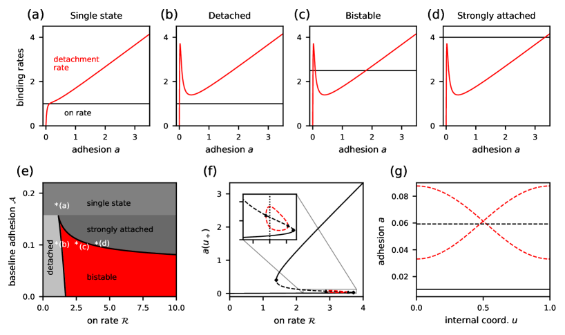
Figure 2: Adhesion-based polarization mechanism without polymerization and for constant stress. (a)-(d) Four qualitatively different scenarios for the local steady state adhesion density depending on the baseline friction $\mathcal{A}$, and the on-rate $\mathcal{R}$ (shown as the black horizontal line). (e) The corresponding phase diagram exhibits four regions, where the thick black line indicates the loci of saddle-node bifurcations. (f) Steady state bifurcation diagram including inhomogeneous solutions. The adhesion density at the leading edge $a(u_{+})$ is shown as a function of the on-rate $\mathcal{R}$, obtained by numerical continuation. Black lines belong to homogeneous states, red ones are associated with polarized states. Solid/dashed lines indicate stable/unstable states. Diamonds represents saddle-node and triangles pitchfork bifurcations. (g) Corresponding adhesion profiles at $\mathcal{R}=3.0$ in (f). Solid/dashed states are stable/unstable.

Fig. 2(a)-(d) illustrates the four qualitatively distinct cases which arise in this situation when varying $\mathcal{R}$ (black horizontal lines) and $\mathcal{A}$, i.e. binding and unbinding. In (a), the unbinding rate increases monotonically with $a$ and the only feasible steady state occurs at the intersection of the two curves at low adhesion. Since the baseline adhesion $\mathcal{A}$ is large, load sharing is suppressed for small $a$. Reducing baseline adhesion $\mathcal{A}$ below a critical value in Fig. 2(b), the detachment rate becomes non-monotonous in $a$ due to load sharing. Nonetheless, with the chosen on-rate $\mathcal{R}=1.0$, only one state is accessible. We term this low adhesion state ”detached”. As the on-rate increases in Fig. 2(c), we enter a regime of multiple solutions through a saddle-node bifurcation. Now the system displays bistability between the detached and a strongly attached state. With an even larger on-rate in Fig. 2(d), only the strongly attached state persists. In Fig. 2(e), we present the full phase diagram. The thick black lines indicate the loci of saddle-node bifurcations, where two solutions emerge, when transitioning from (b) to (c), and, subsequently, annihilate each other from (c) to (d). This analysis is similar to the bifurcation analysis of the standard model for adhesion contacts with mechanosensitive dissociation rates Bell (1978); Erdmann and Schwarz (2004a); Sens (2020), but differs in the existence of a baseline friction.

To investigate the behaviour of steady states in the full, spatially resolved model, we performed numerical continuation of the homogeneous state Doedel et al. (2007). We consider the adhesion density at the right cell edge $a(u_{+})$ in order to capture spatially inhomogeneous and symmetry-broken solutions of equation Eq. 14. In the bifurcation diagram in Fig. 2(f), we plot it as a function of the on-rate $\mathcal{R}$. The black curves represent the discussed homogeneous steady states, where stable (unstable) states are indicated by solid (dashed) lines. The existence of this bistable regime forms the basis of the polarization mechanism presented here: different regions of the cell might be locally in balance either in the detached or attached state. The diffusion term then introduces a spatial coupling and connects these different regions to form smooth adhesion profiles. Because diffusion generally suppresses spatial inhomogeneities, it must be sufficiently slow for such solutions to exist. For the standard value $\mathcal{D}=0.01$ used here, two inhomogeneous branches (red) bifurcate from the unstable homogeneous branch, where the upper (lower) branch is associated with more adhesion at the right (left) edge of the cell. The further the system deviates from the homogeneous state, the stronger the polarization becomes. Corresponding adhesion profiles at $\mathcal{R}=3.0$ are shown in Fig. 2(g), where the adhesion density at the one cell edge exceeds twice that at the other edge.

The emergence of pitchfork bifurcations and the corresponding solutions’ symmetry with respect to the cell’s midpoint, reflects the left-right symmetry inherent in the underlying equations. This symmetry is subsequently spontaneously broken, with stronger polarization as diffusion slows down. As it is typical for diffusive systems, higher order modes with additional peaks emerge when diffusion is reduced further. However, in the context of motility, only the first mode, which is depicted here, is relevant.

So far, our analysis has focused only on adhesion, neglecting its coupling to cell mechanics. Most importantly, the analysis from Fig. 2 indicates that adhesion might lead to rich dynamics. However, if not complemented by other processes, the only stable solution is a sessile state without persistent SSB. Linear stability analysis (not shown) shows that without a finite value of the polymerization velocity $v_{\rm{p}}$, the adhesion density is a second-order effect around the homogeneous stress base state $\sigma(u)=\sigma_{\rm{act}}$. Specifically, adhesion does not influence the steady state cell length $L$. Through finite volume simulations Guyer et al. (2009), we confirmed the global stability of the homogeneous state and observed the expected exponential relaxation in its proximity (not shown), in agreement to previous results without the additional adhesion field Drozdowski et al. (2021). Symmetry broken initial conditions result in a transient directed movement, but the cell eventually comes to a rest because all polarized states are unstable (cf. Fig. 2(g)). We now show that stable SSB and persistent motility can be obtained by combining the binding dynamics analysed above with symmetric edge polymerization.

II.4 Motile solutions in presence of polymerisation

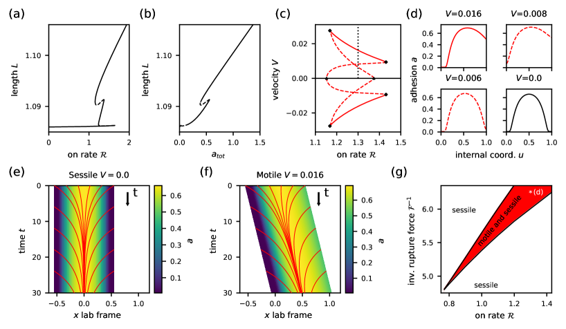
Figure 3: Polymerization stabilizes migration in the full model. (a) Steady state cell length $L$ of sessile states as function of the on-rate $\mathcal{R}$ demonstrates multistability. (b) Cell length $L$ as function of the integrated adhesion density $a_{\rm{tot}}$ shows an overall linear relation, but also multistability. For intermediate adhesiveness, three stable sessile states exist: weakly, moderately and strongly attached. (c) Bistability in the cell velocity $V$ between motile states in red and the three sessile states ($V=0$) in black. Diamonds represent saddle-node and triangles pitchfork bifurcations. (d) Corresponding adhesion profiles at $\mathcal{R}=1.3$. (e) Kymograph of the sessile state. Adhesion density is color-coded and retrograde actin flow is indicated by red lines. (f) Kymograph of the stable motile state. (g) Phase diagram in on-rate $\mathcal{R}$ (”binding”) and inverse rupture force $\mathcal{F}^{-1}$ (”unbinding”) shows bistable region, in which stable migration occurs. Thick black lines indicate the loci of the saddle-node bifurcations on the motile branches (red) in (c).

Now considering the full system, equations Eq. 9-Eq. 13, any finite polymerization velocity $v_{\rm{p}}>0$ induces flow at the boundaries. Consequently, $\partial_{u}\sigma(u)\neq 0$, and a constant stress profile is no longer a valid solution of the problem. The adhesion density then becomes pertinent in the stress equation Eq. 9, in particular impacting the steady state solutions. In this sense, polymerization disrupts the uniform solution and adhesion can emerge as a first order effect around the former uniform steady state. Despite the feedback loop between stress $\sigma$ and adhesion $a$ via the mechanosensitive off-rate, the fundamental structure of steady-state solutions in Fig. 2(f), characterized by the presence of multiple solutions and the appearance of asymmetric branches, remains intact. Therefore, we can understand the mechanism underlying motility based on the analysis in the preceding section.

In Fig. 3(a), the cell length $L$ is depicted as a function of the on-rate $\mathcal{R}$, now with a finite polymerization velocity ($v_{\rm{p}}=0.1$). We observe a similar structural pattern as in Fig. 2(f), where multiple solutions are present within an intermediate range of $\mathcal{R}$. Fig. 3(b) illustrates the relation between $L$ and the total adhesion density $a_{\rm{tot}}=\int_{0}^{1}a(u)\rm{d}u$. For very weak adhesion, the length remains almost independent of $a_{\rm{tot}}$ due to the dominance of baseline friction $\mathcal{A}=0.1$. Toward larger adhesion, length increases nearly linearly with adhesion, i.e. our model correctly predicts spreading of adherent cells on typical culture substrates Reinhart-King et al. (2005). It is worth noting that even for $a_{\rm{tot}}=0$, the steady-state length has increased compared to the case without polymerization. This occurs because both the baseline friction $\mathcal{A}$ and the intrinsic viscosity of the actin network, represented by $\mathcal{L}$, slow down retrograde flow.

Polarized branches are now associated with directed migration. In Fig. 3(c), we illustrate the steady-state velocity $V$ as a function of the on-rate, with motile branches highlighted in red (for reasons of clarity, motile branches are not shown in panel (a) and (b)). In this representation, all symmetric branches collapse to a single line $V=0$. Compared to Fig. 2(f), two saddle-node bifurcations occur on each polarized branch, enclosing a stable region. The corresponding adhesion profiles at $\mathcal{R}=1.3$ are depicted in Fig. 3(d), where only one of the three stable sessile solutions is shown (bottom right in black). Similarly to before, both a detached and a strongly attached state persist as well. Fig. 3(e) and (f) show kymographs of the sessile and motile state, respectively, obtained by finite volume simulations. In both cases, the adhesion profile stays constant over time, confirming that both of them represent steady states of our system. Finally Fig. 3(g) shows the full phase diagram, demonstrating that motile solutions are possible if adhesion is complemented by polymerization.

II.5 Comparision with experimental observations

Our theoretical results are in good qualitative agreement with experimental observations. We first note that our system exhibits true bistability between a motile and multiple sessile states, as observed for different cell types migrating on both 2D substrates Verkhovsky et al. (1999); Barnhart et al. (2011) and on 1D tracks under lateral confinement Hennig et al. (2020); Amiri et al. (2023). The border between the sessile and bistable regime in the phase space diagram in Fig. 3(g) is given by the loci of the saddle-node bifurcations on the motile branches. As explained before, a minimal inverse rupture force $\mathcal{F}^{-1}$ is required to achieve polarization. Because the bistable regime extends along the diagonal in Fig. 3(g), we conclude that binding and unbinding have to be in balance to enable motility. Away from this region, only sessile solutions exist. Below we will investigate switching between these states by applying external perturbations.

We next note that in the stable motile states, adhesion is strongly polarized, with strong adhesion at the front and low adhesion at the back, as observed in experiments Fournier et al. (2010); Barnhart et al. (2015); Schreiber et al. (2021). This asymmetry in adhesion distribution leads to the differential rates of retrograde flow between the front and back regions of the cell, facilitating effective forward propulsion through polymerization-driven membrane protrusion. As new adhesive bonds need time to form in the flow, adhesion density peaks near the cell center. It slightly diminishes toward the leading edge as observed, for instance, in MDA-MB-231 cells Schreiber et al. (2021). Actomyosin contraction and membrane tension drive retrograde flow, surpassing the speed of polymerization at the back of the cell, allowing for efficient rear retraction with minimal adhesive resistance. Upon comparison with unstable states, it becomes apparent that both an overall adhesion polarity and the absence of adhesion at the rear are crucial for sustaining efficient cellular migration.

We finally note that in mesenchymal motility, a biphasic adhesion–velocity relation has been measured across various cell types, representing a universal principle in cell migration, where a maximum migration velocity occurs at intermediate ligand concentrations on the substrate Palecek et al. (1997); Barnhart et al. (2011); Schreiber et al. (2021). In our model, motility is only feasible in a regime of intermediate on-rate $\mathcal{R}$, recapitulating the property of an optimal adhesiveness: if adhesion is too low (detached state), active processes solely generate retrograde flow, but fail to transmit their forces to the substrate. Conversely, excessive adhesion prevents the detachment of adhesive bonds at the rear, resulting in a stalled cell. Accordingly, increasing (decreasing) the polymerization speed, as one of the two force-generating processes, shifts the motile regime to larger (smaller) values of the on-rate. Even minor adjustments in $v_{\rm{p}}$ can significantly impact the range of motility in $\mathcal{R}$ due to the exponential coupling between stress and detachment rate.

III Effect of external perturbations in adhesion

To demonstrate the bistable nature of our model and the role of adhesion in motility initiation, we investigate switching from a sessile to a migrating state by applying an asymmetric perturbation to the adhesion density. This perturbation is implemented in a finite volume simulation by setting the adhesion density to zero over a certain fraction of the cell length at a certain point in time ($t=0$), corresponding to a complete loss of adhesion to the substrate, and observing the temporal evolution. From the experimental perspective, this means to disrupt adhesion without destroying the actin network itself or impair the adhesiveness of the substrate, such that the on-rate $\mathcal{R}$ in our model remains the same.

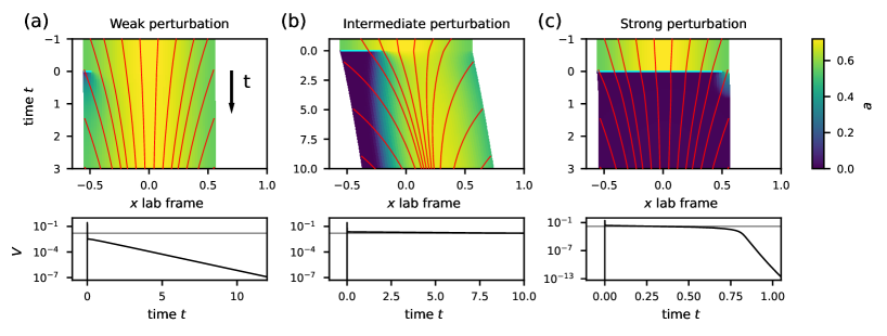
Figure 4: Motility initiation via external perturbation: starting in the strongly attached state, adhesion is destroyed over the left (a) 5 $\%$, (b) 30 $\%$ and (c) 95 $\%$ of the cell length at $t=0$. The upper panels show the corresponding kymographs in the lab frame $x$ with color-coded adhesion density. The actin flow is indicated as red lines, the perturbation as horizontal bars in cyan. Lower panels show the cell velocity as function of time, where the grey line represents the stable migratory steady state.

In Fig. 4(a) adhesion is ”erased” on a small interval of 5 $\%$ of the initial cell length at the left edge. Because friction is drastically reduced in this area, retrograde flow increases and causes a transient, small retraction of this non-adhesive edge (upper panel). This is accompanied by an immediate positive spike in the cell velocity (lower panel), corresponding to the onset of movement to the right, i.e. to the side of stronger adhesion. However, adhesion manages to quickly recover because the overall adhesion density is only slightly affected. The recovery is only possible due to the spatial coupling and the diffusion of adhesion from strongly to weakly attached regions. Simultaneously, the velocity decreases exponentially to zero (lower panel), exactly as one would expect from linear stability analysis in the proximity of a stable state. The velocity actually exceeds the steady migration velocity immediately after the perturbation, but cell length and adhesion profile are too far from the migratory state.

To escape the basin of attraction of the sessile state, the applied perturbation has to be stronger. By disrupting adhesion over 30 $\%$ of the cell length in the prospective rear, as shown in Fig. 4(b), a non-local effect can be seen in the actin flow, which exhibits a kink toward the right even far from the perturbed region. Thus, an overall movement to the right is initiated. Interestingly, the adhesion density on the non-perturbed edge is also reduced because new bonds have to form at the very leading edge during migration, as explained in the previous section. Both effects are facilitated by the non-local coupling of the cell edges through the membrane tension, represented in the symmetric stress BCs Eq. 10. The initial spike in velocity is actually of the same magnitude as for the weak perturbation. However, instead of subsequently decreasing toward zero, it approaches the steady migrating velocity (lower panel). The adhesion recovers to a small degree closer to the cell middle and then develops into the stable state (cf. Fig. 3(d), top left) with a non-adhesive rear and an overall polarization.

A very strong perturbation, where adhesion is erased over 95 $\%$ of the cell length, as investigated in Fig. 4(c), leads again to a initial velocity spike of the same order as for the two previous cases. The cell enters a transient state, during which it migrates with a similar velocity as in (b), but the adhesion profile is quite different. Eventually, the remaining adhesion at the leading tip cannot withstand the active forces and diminishes rapidly, in the shown example around $t=1$. Therefore, the velocity decays exponentially and the movement stops (lower panel). In contrast to panel (a), the cells ends up in the detached state. It should be notedt that the bulk properties are not immediately reflected in the current cell length and velocity right after the perturbation, but they are highly relevant in determining the long-term behaviour and final state. This prediction is only possible in a spatially resolved model and highlights the benefits of our continuum approach compared to previously proposed point-like descriptions.

In conclusion, a sufficiently strong polarization has to be established to switch to the motile state without reducing the overall adhesion density too much. Then, the cell edge losing adhesion becomes the prospective trailing rear. In practise, cells are subject to strong thermal noise Hennig et al. (2020); Amiri et al. (2023), which can cause the switching between states, here shown in a purely deterministic theory. In principle, optogenetics could be used for such manipulations as well and have been recently applied to regulate talin as a mechanical linker in cell-matrix adhesions Sadhanasatish et al. (2023). The instantaneous disruption of adhesion can easily be extended to a time-integrated signal resembling the effect of optogenetics within our framework.

Our observations demonstrate the pivotal role of adhesion in establishing global polarity and initiating motility without previous polarization of the actomyosin system itself. Furthermore, it supports the hypothesis that the cell rear can be defined by sudden detachment Hennig et al. (2020). Because in this purely mechanical model without a direct or indirect positive correlation between polymerization and adhesion assembly, edge polymerization alone would not be able to create a stable leading edge. Even though an asymmetric increase in polymerization would indeed create a transient protrusion and migration in the corresponding direction, the created stresses accelerate adhesion detachment at this side. As soon as polymerization goes back to its symmetric configuration, the movement would stop or even revert. To compensate this effect one could consider catch-bond behaviour for small stresses, where the off-rate decreases under small load, or directly couple adhesion and polymerization. Such an interaction was experimentally observed Vicente-Manzanares et al. (2009) and could be mediated e.g. by the Arp2/3 complex, facilitating both actin polymerization and adhesion formation Goley and Welch (2006); Sever and Schiffer (2018).

IV Effect of patterning adhesion

Finally, we analyse the behaviour of cells in a structured environment, including adhesive steps Barnhart et al. (2011); Schreiber et al. (2021) and continuous gradients of adhesiveness Ricoult et al. (2015). We introduce a spatial dependence of the on-rate and assume that this adhesive cue is substrate-bound and stays constant over time, i.e. it is neither consumed or produced by the cell itself. The guiding by such an adhesive cue is called haptotaxis.

IV.1 Haptotaxis on adhesive gradients

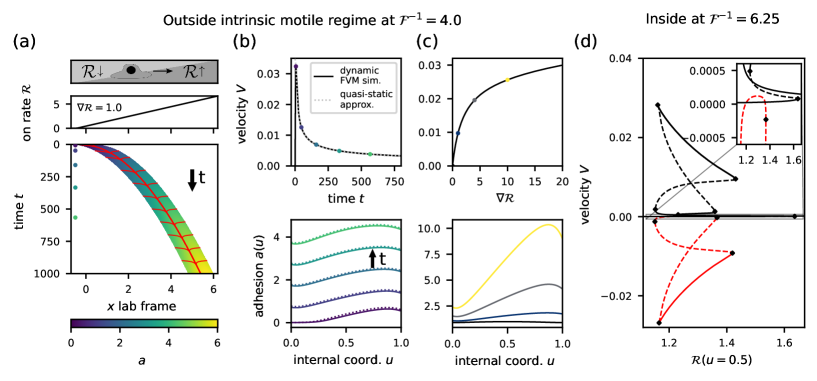
Figure 5: Haptotaxis on continuous gradients. (a)-(c) Outside the intrinsic motile regime. (a) The upper panel shows a sketch of a cell on a constant gradient of the on-rate, which is depicted in the middle panel. The lower panel displays the kymograph with color-coded adhesion density and actin flow in red. (b) Corresponding cell velocity (top) and adhesion profiles at different time points (bottom). The quasi-static approximation is obtained by numerical continuation. (c) Quasi-static approximation of the velocity as a function of the gradient (top) and corresponding adhesion profiles (bottom) for fixed on-rate at the trailing edge of $\mathcal{R}(u_{-})=1.3$. (d) Bifurcation diagram of the steady state velocity $V$ within the intrinsic motile regime for a small external gradient in the on-rate of $\nabla\mathcal{R}=0.01$. The x-axis shows the values of the on-rate at the cell middle $u=0.5$. This perturbation results in imperfect bifurcations (inset) and disconnected branches (black and red).

To demonstrate the basic principles of haptotaxis in our model, we first analyse the behaviour on constant gradients within and outside the intrinsic motile regime. In Fig. 5(a)-(c), we choose a characteristic rupture force of $\mathcal{F}^{-1}=4.0$ such that, regardless of the on-rate, only one sessile state exists (cf. Fig. 3(g)). Nevertheless, the cell is able to follow the gradient in the on-rate uphill (here $\nabla\mathcal{R}=1.0$), because the heterogeneous environment creates polarization within the initially symmetric cell. The lower part of panel (b) shows the adhesion profiles over time. Since the gradient is constant, the polarity and shape of these profiles are almost identical, neglecting an overall adhesion density increase. The cell length increases, while the migration speed (upper panel in (b)) deteriorates. An increased adhesion must be overcome at the cell rear, impeding retraction in the rear. Additionally, larger stress gradients facilitate retrograde flow at both edges. Thus, we observe the same trend as in the motile regime, where the largest velocities occur for the smallest possible on-rate (cf. Fig. 3(c)).

The dynamical behaviour, obtained with finite volume simulations, can be approximated in a ”quasi-static” manner (dashed lines in Fig. 5(b)). Numerical continuation allows us to predict the steady state corresponding to the current environment, namely the gradient and the absolute on-rate e.g. at the cell middle. The cell will never reach this state in a dynamical situation because the absolute on-rate changes permanently during migration. However, since both the velocity curves and adhesion profiles agree very nicely after an initial phase, we can turn the setup in the quasi-static approximation around and predict the velocity and adhesion profiles as a function of the gradient given the absolute on-rate value. The polarity increases with the gradient as expected (cf. lower panel in Fig. 5(c)). However, we observe a nonlinear velocity-gradient relation, where the increase in velocity decreases for larger gradients. The overall growth in adhesion density limits the increase in velocity. In particular, adhesion gets significantly stronger at the trailing edge, even though the on-rate is kept constant there. This is mainly caused by diffusion, which becomes more relevant for larger adhesion values, and to a smaller amount by the effective advection.

Applying a small gradient within the intrinsic motile regime for $\mathcal{F}^{-1}=6.25$ perturbs the bifurcation diagram, as illustrated in Fig. 3(d). Any small but finite gradient breaks the underlying left-right symmetry and, therefore, converts the former pitchfork to imperfect bifurcations, such that the positive and negative velocity branches become disconnected (cf. inset in Fig. 5(d) for $\nabla\mathcal{R}=0.01$). This is accompanied by an overall shift in velocity, in this case upward since the gradient promotes migration to the right. However, the cell can still migrate against such a small gradient. Above a critical value, which is around $\nabla\mathcal{R}\approx 0.1$, this is no longer possible. Interestingly, the maximum possible migration speeds of both intrinsic and externally driven migration as well as their combination are always of the same order of around $0.03$. This highlights the fact that the velocity is determined by the forces generated within the cell, which are in turn controlled by the active processes, which we kept constant here. Thus, even though external cues can steer migration, it is powered by the cell itself.

IV.2 Motility initiation on lines with adhesive steps

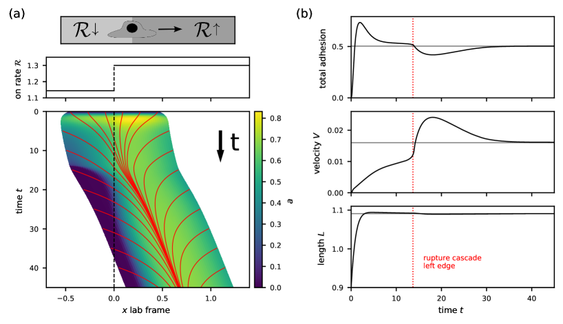
Figure 6: Polarization and motility initiation on an adhesive step. (a) Sketch of the protocol (top), spatially dependent on-rate (middle) and kymograph with color-coded adhesion density and actin flow indicated by red lines (bottom). The cell is initialized without any adhesion and a length of $L=0.9$. (b) Corresponding integrated adhesion density (top), cell velocity $V$ (middle) and cell length $L$ (bottom) as functions of time. Grey lines represent the stable migratory steady state.

After having established the basic haptotactic behaviour of cells preferring stronger adhesiveness, we now consider an initially completely non-adherent cell on top of an adhesive step. This is schematically illustrated in the top panel of Fig. 6(a) with the corresponding on-rate $\mathcal{R}$ below. For the larger on-rate on the right side of the step, the system is within the multistable regime with a stably migrating steady state. On the left side, the system is slightly below the critical value, such that the only available steady state is the detached state. In the beginning at $t=0$, adhesive bonds form almost homogeneously over the complete cell length and spreading occurs symmetrically to both sides due to polymerization, which in turn drives retrograde actin flow. When the cell reaches its maximum length (cf. bottom panel in (b)) and therefore the boundary stress peaks, the adhesion density stagnates and subsequently decreases. However, while on the right side a stable density is achieved, the left half of the cell loses more and more traction. This is accompanied by a slight shift in actin flow to the right, until a critical density on the left edge is reached and a rupture cascade causes the sudden loss of adhesion at the rear, in the shown example at around $t=14$, resulting in a steep increase of velocity. A global polarization has now been established and the cell migrates to the right, as expected.

When the cell gradually enters into a region of higher adhesion density, the non-adhesive rear shrinks in size and overall adhesion rises again. However, even after the cell has completely crossed the step, polarity remains intact in a now homogeneous environment. Therefore, a sufficiently steep step in the correct regime of adhesiveness provides another initiation mechanism to switch into the migratory state. Key to this permanent polarization is that on the less adhesive side only the detached state is available, while the right part is within the motile regime (cf. Fig. 3(c)). Based on our findings in Sec. III on motility initiation via an external perturbation, we conclude that a sufficiently large fraction has to be exposed to the less adhesive region to form the prospective non-adhesive rear. If this was not the case, the cell would still show haptotactic behaviour by sensing and entering the more adhesive region, but would stop right after the step.

IV.3 Motility arrest and direction reversal

After studying motility initiation, we now turn to the opposite process, when a migrating cell approaches a step downwards in adhesiveness. In principle, three distinct scenarios are known from experiments Schreiber et al. (2021); Amiri et al. (2023): the cell continues to migrate in the same direction, the movement is stopped or the direction is reversed under repolarization of the cell.

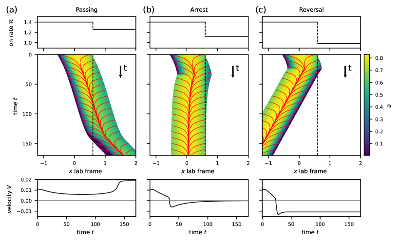
Figure 7: Motility arrest and reversal at an adhesive step. A stably migrating cell approaches a step in the on-rate (top) from $\mathcal{R}=1.4$ down to (a) 90 $\%$, (b) 80 $\%$ and (c) 70 $\%$. Kymographs show color-coded adhesion density and actin flow indicated by red lines. The cell will pass small steps, migration stops for intermediate steps and it is reverted under repolarization of the adhesion density for large steps. The bottom row shows the corresponding cell velocity $V$ over time. The sessile state with $V=0$ is indicated in grey.

All three cases occur in our model, as demonstrated in Fig. 7, depending on the initial migrating state and on the step size. In Fig. 7(a), the on-rate is reduced by 10 $\%$ across the step. While the cell passes the step, the adhesion density is gradually reduced from front to back leading to a transient weakening of the polarization and therefore a reduction of the velocity. Once the cell has completed the step, overall adhesion is obviously less compared to the initial state, but the velocity has increased, in agreement with the bifurcation diagram in Fig. 3(c), where motile states are faster for smaller on-rates.

In Fig. 7(b) we observe a motility arrest for a step size of 20 $\%$. The on-rate of $\mathcal{R}=1.12$ after the step is not within the motile regime anymore, such that complete passing is not achievable. The leading edge transiently crosses into the less adhesive region, similar to the ”passing” case in panel (a). However, adhesion at the cell front is significantly more reduced, facilitating retrograde flow. Thus, protrusion speed is slowed down, even before the polarization is lost, concomitantly with a shortening of the cell length. This in turn reduces the stress at the cell edges, until a critical point around $t=30$. Then, the on-rate excels the off-rate at the rear, leading to a rapid growth in adhesion and an arrest of the directed movement. In agreement with our observation of haptotaxis in the previous section, the unpolarized cell prefers the highly adhesive region and slowly returns to the left side of the step. The observed fast adaptation demonstrates the local cooperativity of adhesive bonds. In contrast to an advective mechanism based on intracellular transport, this allows a cell to sense its environment very fast and efficiently.

For complete repolarization and reversal of direction, the former front of the cell must switch to the detached state. Increasing the step size further to 30 $\%$ leads to the expected effect, as shown in Fig. 7(c): subsequently to the formation of strong adhesion at the former rear, the cell length and the stress at the edges start to grow again, causing a rupture cascade at the right edge and a reversal of actin flow. The repolarized cell migrates in the opposite direction and polarity remains intact after crossing back into a homogeneous environment. Larger steps accelerate the repolarization process but result in the same qualitative behaviour of reversal. This behaviour cannot be predicted solely by the known steady states, since the dynamical length changes play a crucial role, demonstrated by the qualitative difference between (b) and (c), where in both cases the only accessible steady state in the less-adhesive region is the sessile, detached state. However, only in (c) we observe full repolarization. The intricate interplay of length, velocity, and cell fraction beyond the step boundary, with the effected bond rupture behavior, necessitates a one-dimensional representation of the cell. This constitutes a strength of our spatially resolved one-dimensional approach. For every pair of left and right on-rates a dynamical simulation can be conducted to obtain predictions.

V Discussion

In this work, we have shown how active gel theory can be extended by a dynamic adhesion field in a 1D setting. Similarly to the molecular clutch model, actin flow is slowed down by adhesive contacts to the substrate; but differently from standard molecular clutch models, the direction of flow is not assumed, but predicted by our theory. Our model demonstrates that the interplay between local load sharing between mechanosensitive bonds and initially symmetric polymerization-driven retrograde flow leads to spontaneous symmetry breaking. Thus our theory identifies a novel polarization and motility mechanism for 1D cell migration. Because the model gives clear predictions on actin flow and adhesion dynamics, it can be compared directly to experiments. In fact, the predicted ranges of migration speeds and adhesion profiles are in very good agreement with experimental measurements of cells on 1D lines. In agreement with experimental observations, our model exhibits bistability between sessile and motile states. We have demonstrated how local perturbations in adhesion can induce switching and have highlighted the potential role of adhesion in motility initiation. While the adhesion density close to the boundary determines the current edge movement, bulk properties dictate the long-term behaviour and convergence toward a steady state. This distinction is only possible due to our continuum framework.

By introducing a spatial dependence of the binding rate in our model, we are able to describe heterogeneities and especially gradients and steps in substrate adhesiveness. Our model qualitatively captures the haptotactic behaviour of cells to prefer more adhesive regions. On continuous gradients, we have analysed migration within and outside of the intrinsic motile regime. In a quasi-static approximation we have access to the full bifurcation diagram. Predicted velocities and adhesion profiles agree very well with full dynamical simulations. For discontinuous steps in the adhesiveness, we were able to qualitatively reproduce experimentally observed directional reversal and repolarization. While the cooperativity of bonds is very sensitive to local environmental changes, the non-local elastic boundary condition provides a fast communication between both cell ends. Together, these two mechanism allow for a fast decision making on structured patterns. In addition to patterned substrates as external stimulus, direct manipulation of adhesion bonds by means of optogenetics Sadhanasatish et al. (2023) presents another exciting possibility, which could be included in our model, to better understand the dynamic organization of adhesion.

Since we have assumed an active stress that is constant in space and time, actomyosin contraction only acts in the background and does not drive SSB by itself. However, adding a dynamic myosin concentration field, as done e.g. in reference Lo et al. (2024), could lead to more complex behaviour, such as oscillatory stick-slip migration Hennig et al. (2020); Amiri et al. (2023). Furthermore, it would become possible to compare the timescales needed to establish adhesion and myosin polarity. This could greatly enhance our understanding of SSB in real cells and how the different components of the cytoskeleton interact. On the other hand, one could incorporate more details into the binding dynamics, e.g. by considering catch-bond behaviour Marshall et al. (2003); Sens (2020) or mechanosensitive adhesion bond recruitment from reservoirs Braeutigam et al. (2022), which both might play a role in the interplay of actin flow and maturation of focal adhesions Vicente-Manzanares et al. (2009). Finally, it would be interesting to extend the 1D-theory presented here to 2D, for example to describe the movement of keratocytes and lamellipodial fragments Blanch-Mercader and Casademunt (2013); Reeves et al. (2018); Safsten et al. (2022).

Appendix A Derivation of boundary conditions for the adhesion density

We consider two species: bound $a_{\rm{b}}(x,t)$ and unbound $a_{\rm{u}}(x,t)$ adhesion sites. Both densities change due to (un)binding, diffusion and, in addition, unbound sites are advected with the actin gel’s velocity $v$. The dynamic equations then read

$$\partial_{t}a_{\rm{b}} =+\tilde{r}_{\rm{on}}a_{\rm{u}}-r_{\rm{off}}a_{\rm{b}}+D_{\rm{b}}\partial_{x}^{2}a_{\rm{b}},$$ (15)

$$\partial_{t}a_{\rm{u}}+\partial_{x}(va_{\rm{u}}) =-\tilde{r}_{\rm{on}}a_{\rm{u}}+r_{\rm{off}}a_{\rm{b}}+D_{u}\partial_{x}^{2}a_{\rm{u}}.$$ (16)

Without turnover, the total number of adhesion sites $\int_{l_{-}}^{l_{+}}a_{\rm{tot}}dx$, with $a_{\rm{tot}}=a_{\rm{b}}+a_{\rm{u}}$, has to be conserved. To take into account the movement of the boundaries, we have to apply the Leibniz integral rule. Then, the conservation condition implies

$$0 =\frac{d}{dt}\int_{l_{-}}^{l_{+}}a_{\rm{tot}}dx$$ (17)

$$=\dot{l}_{+}a_{\rm{tot}}(l_{+})-\dot{l}_{-}a_{\rm{tot}}(l_{-})+\int_{l_{-}}^{l_{+}}\partial_{t}a_{\rm{tot}}dx.$$ (18)

The local change of the total adhesion density is given by the sum of equations Eq. 15 and Eq. 16. The binding terms cancel each other and we are left with

$$0=\dot{l}_{+}a_{\rm{b}}(l_{+})-\dot{l}_{-}a_{\rm{b}}(l_{-})+D_{\rm{b}}\partial_{x}\left(a_{\rm{b}}(l_{+})-a_{\rm{b}}(l_{-})\right)$$ (19)

$$\qquad+D_{\rm{u}}\partial_{x}\left(a_{\rm{u}}(l_{+})-a_{\rm{u}}(l_{-})\right).$$

Now, assuming an infinite reservoir of unbound sites, as explained in Sec. II, the second line of the above equation can be neglected. As a result, we obtain Robin-type BCs for $a_{\rm{b}}$ at each cell edge

$$\partial_{x}a_{\rm{b}}(l_{\pm})=-\frac{\dot{l}_{\pm}}{D_{\rm{b}}}a_{\rm{b}}(l_{\pm}),$$ (20)

with the ratio of membrane movement and diffusion. By redefining $r_{\rm{on}}=\tilde{k}_{\rm{on}}a_{\rm{u}}$, we obtain Eq. 4 from Eq. 15.

Appendix B Parameter estimates

The following estimates are made for a thin two-dimensional slab of material. The cell is assumed to be homogeneous in the direction orthogonal to its direction of movement, such that our model is effectively a one-dimensional problem. Nevertheless, stresses are still given in units of force per area and bond density is also measured per area. This allows also for easier comparison to experimental measurements.

The cell parameters (cf. Tab. 1 top) are taken from either experimental measurements or from similar models, except for the effective friction coefficient, which is derived below. The off-rate without load $r_{0}$ and the typical rupture force $f_{0}$ of bonds (cf. Tab. 1 bottom) have already been estimated in other models, partly based on experimental measurement. To obtain a reasonable value for the effective friction coefficient $\xi$ in our model, we consider the intermediate friction regime from reference Barnhart et al. (2011), $\tilde{\xi}=10^{15}$ Pa s/m². The typical order of stress in our system is given by the active contractility of $\sigma_{\rm{act}}=10^{3}$ Pa. In a motile state, the force per bond should be in the order of the typical rupture force of $f_{0}$ = 2 pN, such that sufficiently strong binding can occur without stalling the cell. Then, we can estimate the bond density

$$a=\frac{\sigma_{\rm{act}}}{f_{0}}=5\cdot 10^{2}/\mu\rm{m}^{2}.$$ (21)

From this value, we obtain the effective friction coefficient

$$\xi=\frac{\tilde{\xi}}{a}=2\ \rm{Pa\ s}.$$ (22)

Under steady state conditions, binding and unbinding should be balanced

$$r_{\rm{on}}=a\cdot r_{\rm{off}}\approx a\cdot r_{0}=50/(s\ \mu\rm{m}^{2}).$$ (23)

Since we use the on-rate as our continuation parameter, this approximation just provides a rough estimation of the expected order of magnitude.

The baseline bond density $a_{0}$ and the diffusion $D$ are effective parameters, without a direct accessible counterpart in real cells. As discussed in the Sec. II.1, both stabilize the system and are chosen sufficiently small to allow for polarization. The chosen value of $a_{0}=50/\mu\rm{m}^{2}$ would correspond to 10 $\%$ of the expected dynamical adhesion bond density $a$.

Cell parameters
Actin polymerization speed $v_{\rm{p}}$	0.1 $\mu$m/s	measured in Pollard and Borisy (2003); Barnhart et al. (2011)
Cell cortex stiffness $k$	$10^{4}$ Pa	estimated in Recho et al. (2015)
Contractility $\sigma_{\rm{act}}$	$10^{3}$ Pa	used in Recho et al. (2015); Drozdowski et al. (2021) based on Barnhart et al. (2011); Oakes et al. (2017)
Bulk viscosity $\eta$	$10^{5}$ Pa s	estimated in Barnhart et al. (2011); Recho et al. (2015)
Cell rest length $L_{0}$	10 $\mu$m	typical order e.g. in Verkhovsky et al. (1999)
Effective friction coefficient $\xi$	2 Pa s	estimated based on Barnhart et al. (2011)
Bond parameters
On-rate $r_{\rm{on}}$	50 /$\mu\rm{m}^{2}$	estimated in this work,
		similar considerations in Sens (2020)
Off-rate without load $r_{0}$	0.1 s	similar values used in Barnhart et al. (2011); Sens (2020); Ron et al. (2020),
		measured in Lele et al. (2008)
Typical rupture force $f_{0}$	2 pN	measured in Jiang et al. (2003); Bangasser et al. (2013),
		similar values in Sens (2020); Ron et al. (2020)
Baseline bond density $a_{0}$	50 /$\mu\rm{m}^{2}$	estimated in this work
Effective diffusion D	0.1 $\mu$m/s2	estimated in this work,
		similar values used in Barnhart et al. (2011); Chen et al. (2023)

Table 1: Physical parameters assumed in our model.

Cell parameters
Actin polymerization speed $v_{\rm{p}}$	0.1
Contractility $\sigma_{\rm{act}}$	0.1
Relative viscous time scale $\mathcal{L}$	1.0
Bond parameters
On-rate $\mathcal{R}$	continuation parameter, expected range 0.1 - 10.0
Rupture force $\mathcal{F}$	0.1 (0.16 used in simulations)
Baseline bond density $\mathcal{A}$	0.1
Effective diffusion $\mathcal{D}$	0.01

Table 2: Dimensionless parameters derived from the physical parameters given in Tab. 1.

References

- Bodor et al. (2020) D. L. Bodor, W. Pönisch, R. G. Endres, and E. K. Paluch, Developmental Cell 52, 550 (2020).
- Stuelten et al. (2018) C. H. Stuelten, C. A. Parent, and D. J. Montell, Nature Reviews Cancer 18, 296 (2018), number: 5 Publisher: Nature Publishing Group.
- Abercrombie (1980) M. Abercrombie, Proceedings of the Royal Society of London. Series B. Biological Sciences 207, 129 (1980), publisher: Royal Society.
- Verkhovsky et al. (1999) A. B. Verkhovsky, T. M. Svitkina, and G. G. Borisy, Current Biology 9, 11 (1999).
- Ziebert et al. (2012) F. Ziebert, S. Swaminathan, and I. S. Aranson, J. R. Soc. Interface 9, 1084 (2012).
- Lavi et al. (2016) I. Lavi, M. Piel, A.-M. Lennon-Duménil, R. Voituriez, and N. S. Gov, Nature Physics 12, 1146 (2016), publisher: Nature Publishing Group.
- Ron et al. (2020) J. E. Ron, P. Monzo, N. C. Gauthier, R. Voituriez, and N. S. Gov, Physical Review Research 2, 033237 (2020), publisher: American Physical Society.
- Amiri et al. (2023) B. Amiri, J. C. J. Heyn, C. Schreiber, J. O. Rädler, and M. Falcke, Biophysical Journal 122, 753 (2023).
- Maiuri et al. (2012) P. Maiuri, E. Terriac, P. Paul-Gilloteaux, T. Vignaud, K. McNally, J. Onuffer, K. Thorn, P. A. Nguyen, N. Georgoulia, D. Soong, A. Jayo, N. Beil, J. Beneke, J. C. Hong Lim, C. Pei-Ying Sim, Y.-S. Chu, A. Jiménez-Dalmaroni, J.-F. Joanny, J.-P. Thiery, H. Erfle, M. Parsons, T. J. Mitchison, W. A. Lim, A.-M. Lennon-Duménil, M. Piel, and M. Théry, Current Biology 22, R673 (2012).
- Maiuri et al. (2015) P. Maiuri, J.-F. Rupprecht, S. Wieser, V. Ruprecht, O. Bénichou, N. Carpi, M. Coppey, S. De Beco, N. Gov, C.-P. Heisenberg, C. Lage Crespo, F. Lautenschlaeger, M. Le Berre, A.-M. Lennon-Dumenil, M. Raab, H.-R. Thiam, M. Piel, M. Sixt, and R. Voituriez, Cell 161, 374 (2015).
- Hennig et al. (2020) K. Hennig, I. Wang, P. Moreau, L. Valon, S. DeBeco, M. Coppey, Y. A. Miroshnikova, C. Albiges-Rizo, C. Favard, R. Voituriez, and M. Balland, Science Advances 6, eaau5670 (2020).
- Schreiber et al. (2021) C. Schreiber, B. Amiri, J. C. J. Heyn, J. O. Rädler, and M. Falcke, Proceedings of the National Academy of Sciences 118, e2009959118 (2021), publisher: Proceedings of the National Academy of Sciences.
- Kruse et al. (2005) K. Kruse, J. F. Joanny, F. Jülicher, J. Prost, and K. Sekimoto, The European Physical Journal E 16, 5 (2005).
- Jülicher et al. (2007) F. Jülicher, K. Kruse, J. Prost, and J. F. Joanny, Physics Reports Nonequilibrium physics: From complex fluids to biological systems III. Living systems, 449, 3 (2007).
- Prost et al. (2015) J. Prost, F. Jülicher, and J.-F. Joanny, Nature Physics 11, 111 (2015), number: 2 Publisher: Nature Publishing Group.
- Recho et al. (2013) P. Recho, T. Putelat, and L. Truskinovsky, Physical Review Letters 111, 108102 (2013), publisher: American Physical Society.
- Recho et al. (2015) P. Recho, T. Putelat, and L. Truskinovsky, Journal of the Mechanics and Physics of Solids 84, 469 (2015).
- Wittmann et al. (2020) T. Wittmann, A. Dema, and J. van Haren, Current Opinion in Cell Biology Cell Dynamics, 66, 1 (2020).
- Drozdowski et al. (2021) O. M. Drozdowski, F. Ziebert, and U. S. Schwarz, Physical Review E 104, 024406 (2021), publisher: American Physical Society.
- Drozdowski et al. (2023) O. M. Drozdowski, F. Ziebert, and U. S. Schwarz, Communications Physics 6, 1 (2023), number: 1 Publisher: Nature Publishing Group.
- Humphrey et al. (2014) J. D. Humphrey, E. R. Dufresne, and M. A. Schwartz, Nature Reviews Molecular Cell Biology 15, 802 (2014), publisher: Nature Publishing Group.
- Bell (1978) G. I. Bell, Science 200, 618 (1978), publisher: American Association for the Advancement of Science.
- Erdmann and Schwarz (2004a) T. Erdmann and U. S. Schwarz, Physical Review Letters 92, 108102 (2004a), publisher: American Physical Society.
- Sabass and Schwarz (2010) B. Sabass and U. S. Schwarz, Journal of Physics: Condensed Matter 22, 194112 (2010).
- Schwarz and Safran (2013) U. S. Schwarz and S. A. Safran, Reviews of Modern Physics 85, 1327 (2013), publisher: American Physical Society.
- Schallamach (1963) A. Schallamach, Wear 6, 375 (1963).
- Filippov et al. (2004) A. E. Filippov, J. Klafter, and M. Urbakh, Physical Review Letters 92, 135503 (2004), publisher: American Physical Society.
- Sens (2020) P. Sens, Proceedings of the National Academy of Sciences 117, 24670 (2020), publisher: Proceedings of the National Academy of Sciences.
- Chan and Odde (2008) C. E. Chan and D. J. Odde, Science 322, 1687 (2008), publisher: American Association for the Advancement of Science.
- Bangasser et al. (2013) B. Bangasser, S. Rosenfeld, and D. Odde, Biophysical Journal 105, 581 (2013).
- Oria et al. (2017) R. Oria, T. Wiegand, J. Escribano, A. Elosegui-Artola, J. J. Uriarte, C. Moreno-Pulido, I. Platzman, P. Delcanale, L. Albertazzi, D. Navajas, X. Trepat, J. M. García-Aznar, E. A. Cavalcanti-Adam, and P. Roca-Cusachs, Nature 552, 219 (2017), publisher: Nature Publishing Group.
- Elosegui-Artola et al. (2018) A. Elosegui-Artola, X. Trepat, and P. Roca-Cusachs, Trends in Cell Biology 28, 356 (2018).
- Alonso-Matilla et al. (2023) R. Alonso-Matilla, P. P. Provenzano, and D. J. Odde, Biophysical Journal 122, 3369 (2023).
- Lo et al. (2024) J.-Y. Lo, Y.-H. Tseng, and H.-Y. Chen, Physical Review Research 6, 013164 (2024), publisher: American Physical Society.
- Pollard and Borisy (2003) T. D. Pollard and G. G. Borisy, Cell 112, 453 (2003).
- Ridley et al. (2003) A. J. Ridley, M. A. Schwartz, K. Burridge, R. A. Firtel, M. H. Ginsberg, G. Borisy, J. T. Parsons, and A. R. Horwitz, Science (New York, N.Y.) 302, 1704 (2003).
- Cramer (2010) L. P. Cramer, Nature Cell Biology 12, 628 (2010), number: 7 Publisher: Nature Publishing Group.
- Yam et al. (2007) P. T. Yam, C. A. Wilson, L. Ji, B. Hebert, E. L. Barnhart, N. A. Dye, P. W. Wiseman, G. Danuser, and J. A. Theriot, The Journal of Cell Biology 178, 1207 (2007).
- Barnhart et al. (2015) E. Barnhart, K.-C. Lee, G. M. Allen, J. A. Theriot, and A. Mogilner, Proceedings of the National Academy of Sciences 112, 5045 (2015), publisher: Proceedings of the National Academy of Sciences.
- Ricoult et al. (2015) S. G. Ricoult, T. E. Kennedy, and D. Juncker, Frontiers in Bioengineering and Biotechnology 3 (2015).
- Giannone et al. (2009) G. Giannone, R.-M. Mège, and O. Thoumine, Trends in Cell Biology 19, 475 (2009).
- Barnhart et al. (2011) E. L. Barnhart, K.-C. Lee, K. Keren, A. Mogilner, and J. A. Theriot, PLOS Biology 9, e1001059 (2011), publisher: Public Library of Science.
- Löber et al. (2014) J. Löber, F. Ziebert, and I. S. Aranson, Soft Matter 10, 1365 (2014).
- Janeš et al. (2022) J. A. Janeš, C. Monzel, D. Schmidt, R. Merkel, U. Seifert, K. Sengupta, and A.-S. Smith, Physical Review X 12, 031030 (2022), publisher: American Physical Society.
- Erdmann and Schwarz (2004b) T. Erdmann and U. S. Schwarz, The Journal of Chemical Physics 121, 8997 (2004b).
- Zaidel-Bar et al. (2004) R. Zaidel-Bar, M. Cohen, L. Addadi, and B. Geiger, Biochemical Society Transactions 32, 416 (2004).
- Doedel et al. (2007) E. J. Doedel, A. R. Champneys, F. Dercole, T. F. Fairgrieve, Y. A. Kuznetsov, B. Oldeman, R. Paffenroth, B. Sandstede, X. Wang, and C. Zhang, “AUTO-07P: Continuation and bifurcation software for ordinary differential equations,” (2007).
- Guyer et al. (2009) J. E. Guyer, D. Wheeler, and J. A. Warren, Computing in Science & Engineering 11, 6 (2009).
- Reinhart-King et al. (2005) C. A. Reinhart-King, M. Dembo, and D. A. Hammer, Biophysical Journal 89, 676 (2005), publisher: Elsevier.
- Fournier et al. (2010) M. F. Fournier, R. Sauser, D. Ambrosi, J.-J. Meister, and A. B. Verkhovsky, The Journal of Cell Biology 188, 287 (2010).
- Palecek et al. (1997) S. P. Palecek, J. C. Loftus, M. H. Ginsberg, D. A. Lauffenburger, and A. F. Horwitz, Nature 385, 537 (1997), number: 6616 Publisher: Nature Publishing Group.
- Sadhanasatish et al. (2023) T. Sadhanasatish, K. Augustin, L. Windgasse, A. Chrostek-Grashoff, M. Rief, and C. Grashoff, Science Advances 9, eadg3347 (2023), publisher: American Association for the Advancement of Science.
- Vicente-Manzanares et al. (2009) M. Vicente-Manzanares, C. K. Choi, and A. R. Horwitz, Journal of Cell Science 122, 199 (2009).
- Goley and Welch (2006) E. D. Goley and M. D. Welch, Nature Reviews Molecular Cell Biology 7, 713 (2006), publisher: Nature Publishing Group.
- Sever and Schiffer (2018) S. Sever and M. Schiffer, Kidney international 93, 1298 (2018).
- Marshall et al. (2003) B. T. Marshall, M. Long, J. W. Piper, T. Yago, R. P. McEver, and C. Zhu, Nature 423, 190 (2003), publisher: Nature Publishing Group.
- Braeutigam et al. (2022) A. Braeutigam, A. N. Simsek, G. Gompper, and B. Sabass, Nature Communications 13, 2197 (2022).
- Blanch-Mercader and Casademunt (2013) C. Blanch-Mercader and J. Casademunt, Phys. Rev. Lett. 110, 078102 (2013).
- Reeves et al. (2018) C. Reeves, B. Winkler, F. Ziebert, and I. S. Aranson, Communications Physics 1, 1 (2018), publisher: Nature Publishing Group.
- Safsten et al. (2022) C. A. Safsten, V. Rybalko, and L. Berlyand, Phys. Rev. E 105, 024403 (2022).
- Oakes et al. (2017) P. W. Oakes, E. Wagner, C. A. Brand, D. Probst, M. Linke, U. S. Schwarz, M. Glotzer, and M. L. Gardel, Nature Communications 8, 15817 (2017), publisher: Nature Publishing Group.
- Lele et al. (2008) T. P. Lele, C. K. Thodeti, J. Pendse, and D. E. Ingber, Biochemical and Biophysical Research Communications 369, 929 (2008).
- Jiang et al. (2003) G. Jiang, G. Giannone, D. R. Critchley, E. Fukumoto, and M. P. Sheetz, Nature 424, 334 (2003), publisher: Nature Publishing Group.
- Chen et al. (2023) Y. Chen, D. Saintillan, and P. Rangamani, PRX Life 1, 023007 (2023), publisher: American Physical Society.